rotor platforms on pile-groups running through resonance: a comparison between unbounded soil and...

Soil Dynamics and Earthquake Engineering 50 (2013) 151–161

Contents lists available at SciVerse ScienceDirect

Soil Dynamics and Earthquake Engineering

0267-72http://d

* CorrE-m

peter.ru

journal homepage: www.elsevier.com/locate/soildyn

Rotor platforms on pile-groups running through resonance: A comparisonbetween unbounded soil and soil-layers resting on a rigid bedrock

Antonio Cazzani a,*, Peter Ruge a,b

a University of Cagliari, DICAAR—Department of Civil and Environmental Engineering and Architecture, 2, via Marengo, I-09123 Cagliari, Italyb Technische Universität Dresden, Institut Statik und Dynamik der Tragwerke, D-01062 Dresden, Germany

a r t i c l e i n f o

Article history:Received 11 September 2012Received in revised form11 February 2013Accepted 28 February 2013Available online 16 April 2013

Keywords:Soil-foundation-structure interactionFrequency-dependentDynamic stiffnessPadé approximationRotor start up and shut downFrequency-to-time transformation

61/$ - see front matter & 2013 Elsevier Ltd. Ax.doi.org/10.1016/j.soildyn.2013.02.022

esponding author. Tel.: þ39 070 6755420; faxail addresses: [email protected] (A. [email protected] (P. Ruge).

a b s t r a c t

Rotor platforms supported by pile-groups typically run through resonance during start up and shutdown. End-bearing pile-groups resting on a rather stiff underground surface cause additional layer-resonances compared with pile-groups driven into a half-space. On the other hand, the system'seigenfrequencies are accompanied by energy dissipation due to radiation damping. Thus the questionarises, and is treated in this paper, if this radiation damping for end-bearing pile groups is strong enoughto significantly suppress the additional resonance-peaks.

The analysis uses dynamical stiffness coefficients in the frequency-domain for unbounded mediarecently published by Padrón et al. [1]. In order to treat transient excitations a transformation into thetime-domain is necessary and is here realized through a rational representation which has beendescribed and used in [2] but only for pile groups resting in an elastic half-space, which exhibit a muchsmoother behavior (with reference to frequency) than the case treated here.

& 2013 Elsevier Ltd. All rights reserved.

1. Introduction

The interaction of an unbounded soil-domain with an engi-neering structure in case of transient excitations is still a majorchallenge in foundation engineering, as well as in structural andcomputational dynamics. An appropriate modeling of an infinitesoil-domain requires additional tools, besides the Finite ElementMethod (FEM), in order to avoid a huge grid of elements with anenormous amount of degrees-of-freedom (DOFs).

Indeed, the soil is much more complex than a homogeneousmaterial and such is its numerical treatment as it has been shown,for example, for a piled embankment in Jenck et al. [3]. Nevertheless,results from parametric studies for an idealized homogeneous soilmay show useful tendencies and provide the designing engineerwith helpful insights.

Today, two powerful methods for the dynamical treatment ofunbounded soil domains are used: the Boundary Element Method(BEM), and the Scaled Boundary Finite Element Method (SBFEM).An overview of several applications in civil engineering has beenprepared by Lehmann [4].

These methods solve the problem in the frequency-domainassuming harmonic state variables zðtÞ ¼ z exp ðiΩtÞ with Ωdenoting the angular frequency.

ll rights reserved.

: þ39 070 6755418.zani),

Here and in the following a hat (like z) indicates quantities inthe frequency-domain. Both methods, BEM and SBFEM, end upwith sets of dynamic stiffness (impedance) matrices K or compli-ance (admittance) matrices C coupling the generalized forces fcand the generalized displacements uc in the interface between thesoil and the foundation platform:

f c ¼Kcuc , uc ¼ Cc f c: ð1ÞIn Eq. (1) the generalized displacement vector has the followingform: uT

c ¼ ½u1 … unc �, where nc is the number of DOFs of theinterface. Of course, Eq. (1) is based on assuming harmonicquantities for both state variables:

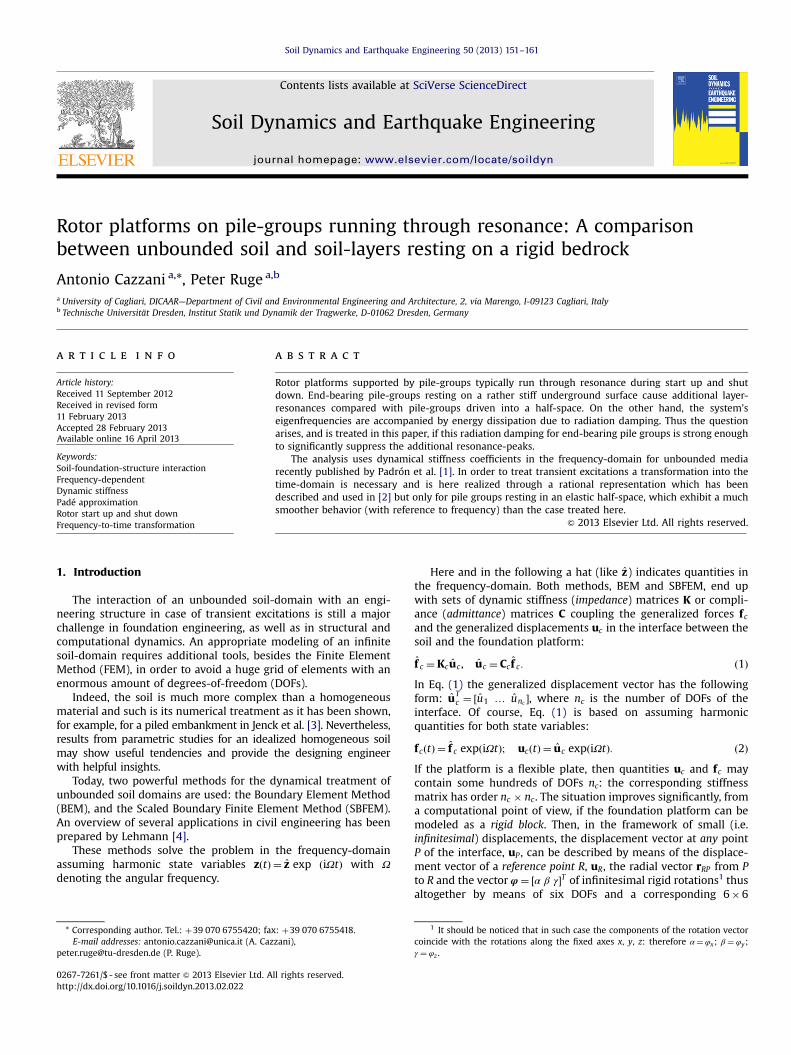
fcðtÞ ¼ f c expðiΩtÞ; ucðtÞ ¼ uc expðiΩtÞ: ð2ÞIf the platform is a flexible plate, then quantities uc and fc maycontain some hundreds of DOFs nc: the corresponding stiffnessmatrix has order nc � nc. The situation improves significantly, froma computational point of view, if the foundation platform can bemodeled as a rigid block. Then, in the framework of small (i.e.infinitesimal) displacements, the displacement vector at any pointP of the interface, uP , can be described by means of the displace-ment vector of a reference point R, uR, the radial vector rRP from Pto R and the vector φ¼ ½α β γ�T of infinitesimal rigid rotations1 thusaltogether by means of six DOFs and a corresponding 6�6

1 It should be noticed that in such case the components of the rotation vectorcoincide with the rotations along the fixed axes x, y, z: therefore α¼ φx; β¼ φy;γ ¼ φz .

www.elsevier.com/locate/soildyn

www.elsevier.com/locate/soildyn

http://dx.doi.org/10.1016/j.soildyn.2013.02.022



mailto:[email protected]

mailto:[email protected]


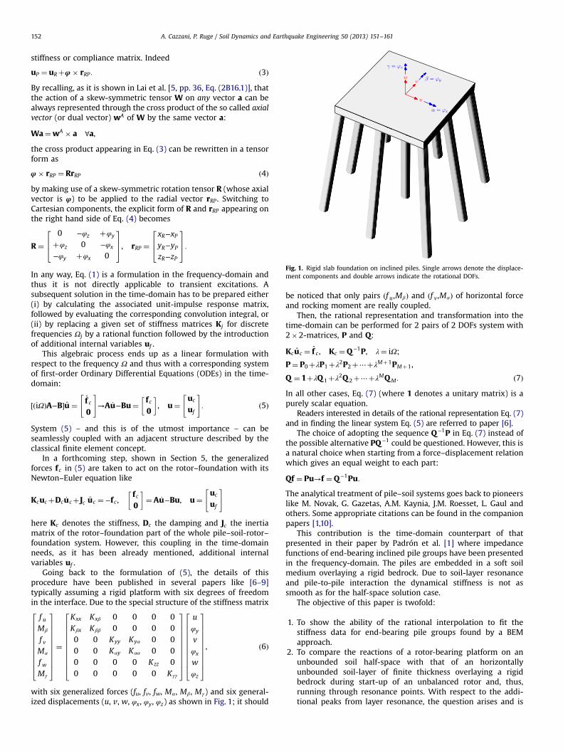
Fig. 1. Rigid slab foundation on inclined piles. Single arrows denote the displace-ment components and double arrows indicate the rotational DOFs.

A. Cazzani, P. Ruge / Soil Dynamics and Earthquake Engineering 50 (2013) 151–161152

stiffness or compliance matrix. Indeed

uP ¼ uRþφ� rRP : ð3ÞBy recalling, as it is shown in Lai et al. [5, pp. 36, Eq. (2B16.1)], thatthe action of a skew-symmetric tensor W on any vector a can bealways represented through the cross product of the so called axialvector (or dual vector) wA of W by the same vector a:

Wa¼wA � a ∀a,

the cross product appearing in Eq. (3) can be rewritten in a tensorform as

φ� rRP ¼ RrRP ð4Þby making use of a skew-symmetric rotation tensor R (whose axialvector is φ) to be applied to the radial vector rRP . Switching toCartesian components, the explicit form of R and rRP appearing onthe right hand side of Eq. (4) becomes

R¼0 −φz þφy

þφz 0 −φx

−φy þφx 0

264

375, rRP ¼

xR−xPyR−yPzR−zP

264

375:

In any way, Eq. (1) is a formulation in the frequency-domain andthus it is not directly applicable to transient excitations. Asubsequent solution in the time-domain has to be prepared either(i) by calculating the associated unit-impulse response matrix,followed by evaluating the corresponding convolution integral, or(ii) by replacing a given set of stiffness matrices Kj for discretefrequencies Ωj by a rational function followed by the introductionof additional internal variables uf .

This algebraic process ends up as a linear formulation withrespect to the frequency Ω and thus with a corresponding systemof first-order Ordinary Differential Equations (ODEs) in the time-domain:

½ðiΩÞA−B�u ¼ f c0

" #→A _u−Bu¼ fc

0

� �, u¼

uc

uf

" #: ð5Þ

System (5) – and this is of the utmost importance – can beseamlessly coupled with an adjacent structure described by theclassical finite element concept.

In a forthcoming step, shown in Section 5, the generalizedforces fc in (5) are taken to act on the rotor–foundation with itsNewton–Euler equation like

KcucþDc _ucþ Jc €uc ¼−fc ,fc0

� �¼ A _u−Bu, u¼

uc

uf

" #

here Kc denotes the stiffness, Dc the damping and Jc the inertiamatrix of the rotor–foundation part of the whole pile–soil-rotor–foundation system. However, this coupling in the time-domainneeds, as it has been already mentioned, additional internalvariables uf .

Going back to the formulation of (5), the details of thisprocedure have been published in several papers like [6–9]typically assuming a rigid platform with six degrees of freedomin the interface. Due to the special structure of the stiffness matrix

f uMβ

f vMα

f wMγ

26666666664

37777777775¼

Kxx Kxβ 0 0 0 0Kβx Kββ 0 0 0 00 0 Kyy Kyα 0 00 0 Kαy Kαα 0 00 0 0 0 Kzz 00 0 0 0 0 Kγγ

26666666664

37777777775

u

φy

v

φx

w

φz

26666666664

37777777775, ð6Þ

with six generalized forces (fu, fv, fw, Mα, Mβ , Mγ) and six general-ized displacements (u, v, w, φx, φy, φz) as shown in Fig. 1; it should

be noticed that only pairs ðf u,MβÞ and ðf v,MαÞ of horizontal forceand rocking moment are really coupled.

Then, the rational representation and transformation into thetime-domain can be performed for 2 pairs of 2 DOFs system with2�2-matrices, P and Q:

Kcuc ¼ f c , Kc ¼Q−1P, λ¼ iΩ;

P¼ P0þλP1þλ2P2þ⋯þλMþ1PMþ1,

Q ¼ 1þλQ 1þλ2Q 2þ⋯þλMQM : ð7ÞIn all other cases, Eq. (7) (where 1 denotes a unitary matrix) is apurely scalar equation.

Readers interested in details of the rational representation Eq. (7)and in finding the linear system Eq. (5) are referred to paper [6].

The choice of adopting the sequence Q−1P in Eq. (7) instead ofthe possible alternative PQ−1 could be questioned. However, this isa natural choice when starting from a force–displacement relationwhich gives an equal weight to each part:

Qf ¼ Pu→f ¼Q−1Pu:

The analytical treatment of pile–soil systems goes back to pioneerslike M. Novak, G. Gazetas, A.M. Kaynia, J.M. Roesset, L. Gaul andothers. Some appropriate citations can be found in the companionpapers [1,10].

This contribution is the time-domain counterpart of thatpresented in their paper by Padrón et al. [1] where impedancefunctions of end-bearing inclined pile groups have been presentedin the frequency-domain. The piles are embedded in a soft soilmedium overlaying a rigid bedrock. Due to soil-layer resonanceand pile-to-pile interaction the dynamical stiffness is not assmooth as for the half-space solution case.

The objective of this paper is twofold:

1.
To show the ability of the rational interpolation to fit thestiffness data for end-bearing pile groups found by a BEMapproach.
2.
To compare the reactions of a rotor-bearing platform on anunbounded soil half-space with that of an horizontallyunbounded soil-layer of finite thickness overlaying a rigidbedrock during start-up of an unbalanced rotor and, thus,running through resonance points. With respect to the addi-tional peaks from layer resonance, the question arises and is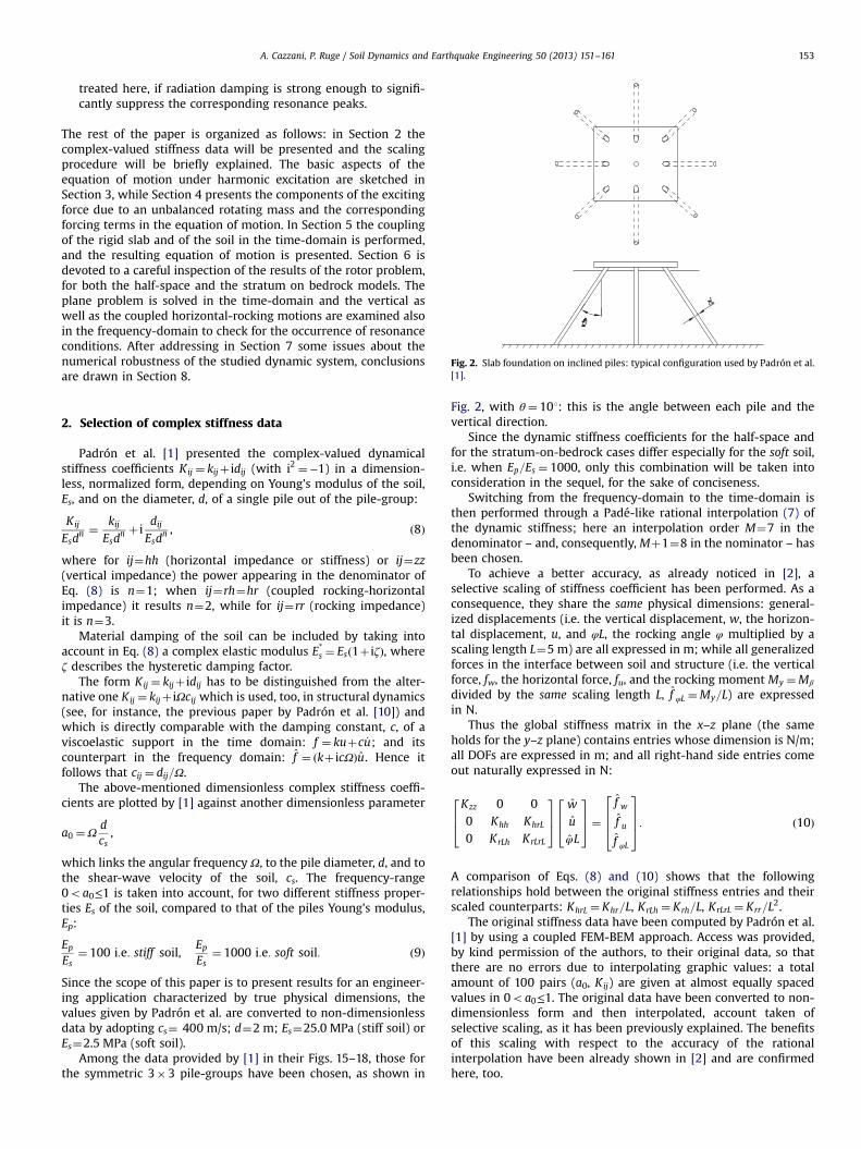

Fig. 2. Slab foundation on inclined piles: typical configuration used by Padrón et al.[1].

A. Cazzani, P. Ruge / Soil Dynamics and Earthquake Engineering 50 (2013) 151–161 153

treated here, if radiation damping is strong enough to signifi-cantly suppress the corresponding resonance peaks.

The rest of the paper is organized as follows: in Section 2 thecomplex-valued stiffness data will be presented and the scalingprocedure will be briefly explained. The basic aspects of theequation of motion under harmonic excitation are sketched inSection 3, while Section 4 presents the components of the excitingforce due to an unbalanced rotating mass and the correspondingforcing terms in the equation of motion. In Section 5 the couplingof the rigid slab and of the soil in the time-domain is performed,and the resulting equation of motion is presented. Section 6 isdevoted to a careful inspection of the results of the rotor problem,for both the half-space and the stratum on bedrock models. Theplane problem is solved in the time-domain and the vertical aswell as the coupled horizontal-rocking motions are examined alsoin the frequency-domain to check for the occurrence of resonanceconditions. After addressing in Section 7 some issues about thenumerical robustness of the studied dynamic system, conclusionsare drawn in Section 8.

2. Selection of complex stiffness data

Padrón et al. [1] presented the complex-valued dynamicalstiffness coefficients Kij ¼ kijþ idij (with i2 ¼−1) in a dimension-less, normalized form, depending on Young's modulus of the soil,Es, and on the diameter, d, of a single pile out of the pile-group:

Kij

Esdn ¼ kij

Esdn þ i

dijEsd

n , ð8Þ

where for ij¼hh (horizontal impedance or stiffness) or ij¼zz(vertical impedance) the power appearing in the denominator ofEq. (8) is n¼1; when ij¼rh¼hr (coupled rocking-horizontalimpedance) it results n¼2, while for ij¼rr (rocking impedance)it is n¼3.

Material damping of the soil can be included by taking intoaccount in Eq. (8) a complex elastic modulus E*s ¼ Esð1þ iζÞ, whereζ describes the hysteretic damping factor.

The form Kij ¼ kijþ idij has to be distinguished from the alter-native one Kij ¼ kijþ iΩcij which is used, too, in structural dynamics(see, for instance, the previous paper by Padrón et al. [10]) andwhich is directly comparable with the damping constant, c, of aviscoelastic support in the time domain: f ¼ kuþc _u; and itscounterpart in the frequency domain: f ¼ ðkþ icΩÞu. Hence itfollows that cij ¼ dij=Ω.

The above-mentioned dimensionless complex stiffness coeffi-cients are plotted by [1] against another dimensionless parameter

a0 ¼Ωdcs,

which links the angular frequency Ω, to the pile diameter, d, and tothe shear-wave velocity of the soil, cs. The frequency-range0oa0≤1 is taken into account, for two different stiffness proper-ties Es of the soil, compared to that of the piles Young's modulus,Ep:

EpEs

¼ 100 i:e: stiff soil,EpEs

¼ 1000 i:e: soft soil: ð9Þ

Since the scope of this paper is to present results for an engineer-ing application characterized by true physical dimensions, thevalues given by Padrón et al. are converted to non-dimensionlessdata by adopting cs¼ 400 m/s; d¼2 m; Es¼25.0 MPa (stiff soil) orEs¼2.5 MPa (soft soil).

Among the data provided by [1] in their Figs. 15–18, those forthe symmetric 3�3 pile-groups have been chosen, as shown in

Fig. 2, with θ¼ 101: this is the angle between each pile and thevertical direction.

Since the dynamic stiffness coefficients for the half-space andfor the stratum-on-bedrock cases differ especially for the soft soil,i.e. when Ep=Es ¼ 1000, only this combination will be taken intoconsideration in the sequel, for the sake of conciseness.

Switching from the frequency-domain to the time-domain isthen performed through a Padé-like rational interpolation (7) ofthe dynamic stiffness; here an interpolation order M¼7 in thedenominator – and, consequently, Mþ1¼8 in the nominator – hasbeen chosen.

To achieve a better accuracy, as already noticed in [2], aselective scaling of stiffness coefficient has been performed. As aconsequence, they share the same physical dimensions: general-ized displacements (i.e. the vertical displacement, w, the horizon-tal displacement, u, and φL, the rocking angle φ multiplied by ascaling length L¼5 m) are all expressed in m; while all generalizedforces in the interface between soil and structure (i.e. the verticalforce, fw, the horizontal force, fu, and the rocking moment My ¼Mβ

divided by the same scaling length L, f φL ¼My=L) are expressedin N.

Thus the global stiffness matrix in the x–z plane (the sameholds for the y–z plane) contains entries whose dimension is N/m;all DOFs are expressed in m; and all right-hand side entries comeout naturally expressed in N:

Kzz 0 00 Khh KhrL

0 KrLh KrLrL

264

375

w

uφL

264

375¼

f wf uf φL

2664

3775: ð10Þ

A comparison of Eqs. (8) and (10) shows that the followingrelationships hold between the original stiffness entries and theirscaled counterparts: KhrL ¼ Khr=L, KrLh ¼ Krh=L, KrLrL ¼ Krr=L

2.The original stiffness data have been computed by Padrón et al.

[1] by using a coupled FEM-BEM approach. Access was provided,by kind permission of the authors, to their original data, so thatthere are no errors due to interpolating graphic values: a totalamount of 100 pairs (a0, Kij) are given at almost equally spacedvalues in 0oa0≤1. The original data have been converted to non-dimensionless form and then interpolated, account taken ofselective scaling, as it has been previously explained. The benefitsof this scaling with respect to the accuracy of the rationalinterpolation have been already shown in [2] and are confirmedhere, too.

Fig. 3. Dynamic stiffness coefficients for vertical motion for piles inclined at 101: half-space (on the left) and stratum on bedrock solution (on the right). Real part (in blue)and imaginary part (in red) of complex stiffness Kzz. Solid lines show the assigned stiffness, isolated dots the Padé approximated values. (For interpretation of the referencesto color in this figure legend, the reader is referred to the web version of this article.)

Fig. 4. Dynamic stiffness coefficients for horizontal motion for piles inclined at 101: half-space (on the left) and stratum on bedrock solution (on the right). Real part (in blue)and imaginary part (in red) of complex stiffness Khh. Solid lines show the assigned stiffness, isolated dots the Padé approximated values. (For interpretation of the referencesto color in this figure legend, the reader is referred to the web version of this article.)

Fig. 5. Dynamic stiffness coefficients for rockingmotion for piles inclined at 101: half-space (on the left) and stratum on bedrock solution (on the right). Values are scaled andcorresponding to a scaling length L¼5 m. Real part (in blue) and imaginary part (in red) of complex stiffness KrLrL . Solid lines show the assigned stiffness, isolated dots thePadé approximated values. (For interpretation of the references to color in this figure legend, the reader is referred to the web version of this article.)


Original and interpolated data are shown together for thevertical stiffness, Kzz, in Fig. 3; for the horizontal stiffness, Khh, inFig. 4; for the scaled rocking stiffness, KrLrL, in Fig. 5; and for thescaled coupled horizontal-rocking stiffness, KrLh, in Fig. 6.

In order to distinguish the data, the original values are shownby a continuous, solid line. The corresponding rational approxima-tion – which is a priori a continuous function – is shown by meansof distinct points only at those frequency values where the

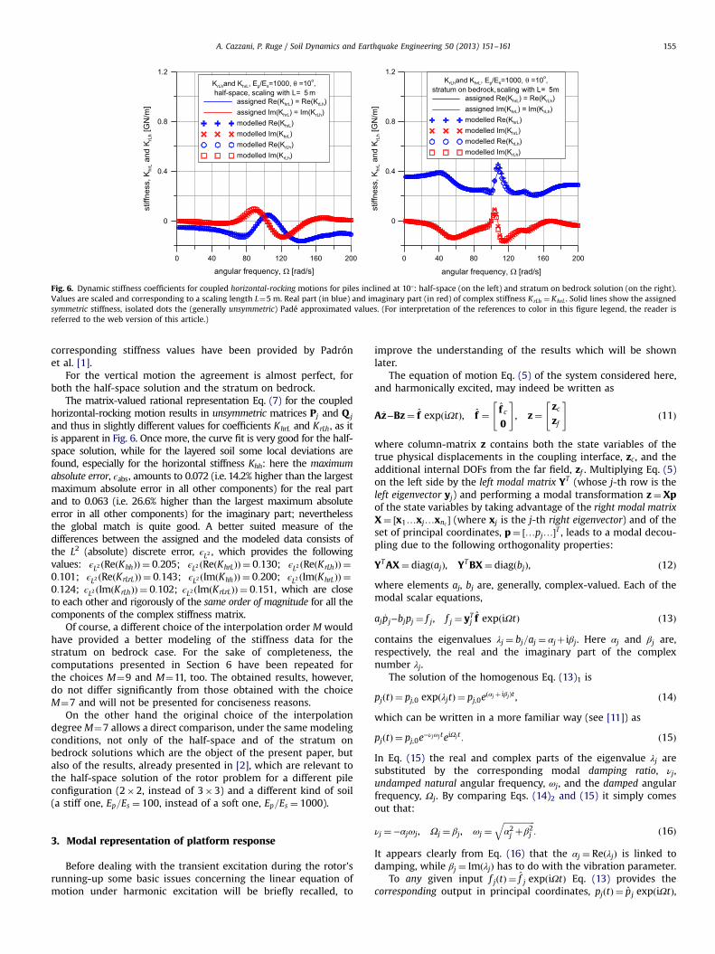
Fig. 6. Dynamic stiffness coefficients for coupled horizontal-rocking motions for piles inclined at 101: half-space (on the left) and stratum on bedrock solution (on the right).Values are scaled and corresponding to a scaling length L¼5 m. Real part (in blue) and imaginary part (in red) of complex stiffness KrLh ¼ KhrL . Solid lines show the assignedsymmetric stiffness, isolated dots the (generally unsymmetric) Padé approximated values. (For interpretation of the references to color in this figure legend, the reader isreferred to the web version of this article.)


corresponding stiffness values have been provided by Padrónet al. [1].

For the vertical motion the agreement is almost perfect, forboth the half-space solution and the stratum on bedrock.

The matrix-valued rational representation Eq. (7) for the coupledhorizontal-rocking motion results in unsymmetric matrices Pj and Q j

and thus in slightly different values for coefficients KhrL and KrLh, as itis apparent in Fig. 6. Once more, the curve fit is very good for the half-space solution, while for the layered soil some local deviations arefound, especially for the horizontal stiffness Khh: here the maximumabsolute error, ϵabs, amounts to 0.072 (i.e. 14.2% higher than the largestmaximum absolute error in all other components) for the real partand to 0.063 (i.e. 26.6% higher than the largest maximum absoluteerror in all other components) for the imaginary part; neverthelessthe global match is quite good. A better suited measure of thedifferences between the assigned and the modeled data consists ofthe L2 (absolute) discrete error, ϵL2 , which provides the followingvalues: ϵL2 ðReðKhhÞÞ ¼ 0:205; ϵL2 ðReðKhrLÞÞ ¼ 0:130; ϵL2 ðReðKrLhÞÞ ¼0:101; ϵL2 ðReðKrLrLÞÞ ¼ 0:143; ϵL2 ðImðKhhÞÞ ¼ 0:200; ϵL2 ðImðKhrLÞÞ ¼0:124; ϵL2 ðImðKrLhÞÞ ¼ 0:102; ϵL2 ðImðKrLrLÞÞ ¼ 0:151, which are closeto each other and rigorously of the same order of magnitude for all thecomponents of the complex stiffness matrix.

Of course, a different choice of the interpolation order M wouldhave provided a better modeling of the stiffness data for thestratum on bedrock case. For the sake of completeness, thecomputations presented in Section 6 have been repeated forthe choices M¼9 and M¼11, too. The obtained results, however,do not differ significantly from those obtained with the choiceM¼7 and will not be presented for conciseness reasons.

On the other hand the original choice of the interpolationdegreeM¼7 allows a direct comparison, under the same modelingconditions, not only of the half-space and of the stratum onbedrock solutions which are the object of the present paper, butalso of the results, already presented in [2], which are relevant tothe half-space solution of the rotor problem for a different pileconfiguration (2�2, instead of 3�3) and a different kind of soil(a stiff one, Ep=Es ¼ 100, instead of a soft one, Ep=Es ¼ 1000).

3. Modal representation of platform response

Before dealing with the transient excitation during the rotor'srunning-up some basic issues concerning the linear equation ofmotion under harmonic excitation will be briefly recalled, to

improve the understanding of the results which will be shownlater.

The equation of motion Eq. (5) of the system considered here,and harmonically excited, may indeed be written as

A _z−Bz¼ f expðiΩtÞ, f ¼ f c0

" #, z¼

zczf

" #ð11Þ

where column-matrix z contains both the state variables of thetrue physical displacements in the coupling interface, zc, and theadditional internal DOFs from the far field, zf . Multiplying Eq. (5)on the left side by the left modal matrix YT (whose j-th row is theleft eigenvector yj) and performing a modal transformation z¼Xpof the state variables by taking advantage of the right modal matrixX¼ ½x1…xj…xnc � (where xj is the j-th right eigenvector) and of theset of principal coordinates, p¼ ½…pj…�T , leads to a modal decou-pling due to the following orthogonality properties:

YTAX¼ diagðajÞ, YTBX¼ diagðbjÞ, ð12Þ

where elements aj, bj are, generally, complex-valued. Each of themodal scalar equations,

aj _pj−bjpj ¼ f j, f j ¼ yTj f expðiΩtÞ ð13Þ

contains the eigenvalues λj ¼ bj=aj ¼ αjþ iβj. Here αj and βj are,respectively, the real and the imaginary part of the complexnumber λj.

The solution of the homogenous Eq. (13)1 is

pjðtÞ ¼ pj,0 expðλjtÞ ¼ pj,0eðαj þ iβjÞt , ð14Þ

which can be written in a more familiar way (see [11]) as

pjðtÞ ¼ pj,0e−νjωj teiΩj t : ð15Þ

In Eq. (15) the real and complex parts of the eigenvalue λj aresubstituted by the corresponding modal damping ratio, νj,undamped natural angular frequency, ωj, and the damped angularfrequency, Ωj. By comparing Eqs. (14)2 and (15) it simply comesout that:

νj ¼ −αjωj, Ωj ¼ βj, ωj ¼ffiffiffiffiffiffiffiffiffiffiffiffiffiffiffiα2j þβ2j

q: ð16Þ

It appears clearly from Eq. (16) that the αj ¼ ReðλjÞ is linked todamping, while βj ¼ ImðλjÞ has to do with the vibration parameter.

To any given input f jðtÞ ¼ f j expðiΩtÞ Eq. (13) provides thecorresponding output in principal coordinates, pjðtÞ ¼ pj expðiΩtÞ,

Figfor


where

pj ¼f jaj

1αjþ iðΩ−βjÞ

" #¼ f j

aj

αj−iðΩ−βjÞα2j þðΩ−βjÞ2

" #: ð17Þ

By Eq. (17) the final solution in the time-domain (i.e. in the originalspace) can be reconstructed:

z¼∑jxj

f jaj

αj−iðΩ−βjÞα2j þðΩ−βjÞ2

" #expðiΩtÞ, aj ¼ yTj Axj, ð18Þ

once appropriate initial conditions are assigned.Obviously, in the occurrence of resonance condition with Ω¼ βj

not only the magnitude of the corresponding damping, νj ¼ αj= ‖λj‖,plays a significant role, but also the modal content of the excitation,f j ¼ yTj f . In other words, even if resonance occurs when Ω¼ βk forsome eigenfrequency βk, (i.e. corresponding to the eigenvalueλk ¼ αkþ iβk), another contribution, with λj ¼ αjþ iβj, can have evenmore influence if βj is near to Ω, νj is rather small (if compared to νk),

and the modal content f j ¼ yTj f is larger than f k ¼ yTk f .

Of course, Eq. (18) provides the solution only for a harmonicexcitation, and not for the more complicated case of an unba-lanced rotor running through resonance, but the global behavior inthe latter case is still comparable to the former one. The mostspecific characteristic of the transient excitation concerns theresonance frequency, Ωres, exhibiting the largest modal amplifica-tion. Resonance occurs with some delay after the eigenfrequencyβj has passed and the amplitude decreases with an increasingangular acceleration of the rotor.

Some more typical results for constantly accelerated rotors arereported in Markert [12].

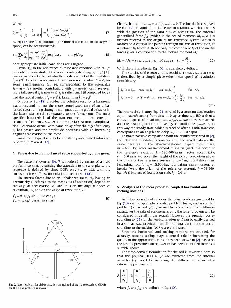
4. Forces due to an unbalanced rotor supported by a pile group

The system shown in Fig. 7 is modeled by means of a rigidplatform, so that, restricting the attention to the x−z plane, theresponse is defined by three DOFs only (u, w, φL), with thecorresponding stiffness formulation given in Eq. (10).

The inertia forces due to an unbalanced mass, mr, having aneccentricity e (referred to the mass axis of revolution) depend onthe angular acceleration, βr , and thus on the angular speed ofrevolution, ωr , and on the angle of revolution, ψ:

f u ¼mrerðβr sin ψþω2r cos ψ Þ

f w ¼mrerðβr cos ψ−ω2r sin ψÞ: ð19Þ

. 7. Rotor problem for slab foundation on inclined piles: the selected set of DOFsthe plane problem is shown.

Clearly, it results: ωr ¼ _ψ and βr ¼ _ωr ¼ ψ... The inertia forces given

by Eq. (19) are applied to the center of rotation, which coincideswith the position of the rotor axis of revolution. The externalgeneralized force f φL (which is the scaled moment, Mβ ¼My) isinstead referred to the origin of the reference system, which islocated on a vertical line passing through the axis of revolution, ata distance hr below it. Hence only the component fu of the inertiaforces gives a contribution to the rocking moment My:

My ¼ f xhr ¼mrerhrðβr sin ψþω2r cos ψÞ, f φL ¼

My

L: ð20Þ

With these ingredients, Eq. (10) is completely defined.The starting of the rotor and its reaching a steady state at t ¼ tE

is described by a simple piece-wise linear speed of revolutiontime-history:

βrðtÞ ¼ βr0, ωrðtÞ ¼ βr0t, ψðtÞ ¼ βr0t2

2for t≤tE

βrðtÞ ¼ 0, ωrðtÞ ¼ βr0tE , ψðtÞ ¼ βr0tE t−tE2

� �for tE≤t≤tF ,

8>>><>>>:

ð21Þ

The rotor's time-history, Eq. (21) is ruled by a constant accelerationβr0 ¼ 1 rad=s2; acting from time t¼0 up to time tE¼180 s; then aconstant speed of revolution ωrE ¼ βr0tE ¼ 180 rad=s is reached,and the resulting motion is investigated until time tF¼250 s. Inthis way the steady state, which is reached after a 3 min transient,corresponds to an angular velocity ωrE ¼ 1718:87 rpm.

To make possible comparison with the results presented in [2],the rotor and foundation geometric and mechanical data are thesame here as in the above-mentioned paper: rotor mass,mr ¼ 6000 kg; rotor mass-moment of inertia (w.r.t. the origin ofthe reference system), Jr ¼ 196,000 kg m2; rotor eccentricity,er ¼ 5=6 mm. Moreover the height of the axis of revolution abovethe origin of the reference system is hr¼5 m; foundation mass(excluding rotor), mf ¼ 18,000 kg; foundation mass-moment ofinertia (w.r.t. the origin of the reference system), Jf ¼ 59,960kg m2; thickness of foundation slab, hf¼0.4 m.

5. Analysis of the rotor problem: coupled horizontal androcking motions

As it has been already shown, the plane problem governed byEq. (10) can be split into a scalar problem for w, and a coupledproblem (for u and φL) governed by a 2�2 complex stiffness-matrix. For the sake of conciseness, only the latter problem will beconsidered in detail in the sequel. However, the equation corre-sponding to (25) for the vertical motion w(t) can be easily derivedin a similar way, provided that all rotational contributions corre-sponding to the rocking DOF φ are eliminated.

Since the horizontal and rocking motions are coupled, foraccuracy reasons scaling plays a crucial role in increasing thequality of the approximation, as it has been shown in [2]. Based onthe results presented there, L¼5 m has been identified here as asuitable choice.

The time-domain formulation for the soil is rewritten here sothat the physical DOFs u, φL are extracted from the internalvariables (zf ), used for modeling the stiffness by means of arational approximation

A

_u_φL_zf

264

375−B

u

φL

zf

264

375¼

f uf φL0

264

375, ð22Þ

where fu and f φL are defined in Eq. (10).


Finally the inertia forces caused by the rigid foundation plateand the rotor itself

f uf φL

" #inertia

¼ Ju..

φ..L

" #, J¼

mt St=L

St=L Jt=L2

" #, ð23Þ

are added to the right side of Eq. (22). Here mt ¼mrþmf is thetotal mass of the system, St the total first-order mass-moment, Jtthe total mass-moment of inertia, both measured with referenceto the foundation base:

St ¼mrhrþmf hf2

, Jt ¼ Jrþ Jf : ð24Þ

In this way, a system of second-order ODEs is obtained; to convertit into a system of first-order ODEs two new variables must beintroduced, namely, vx ¼ _u and ωyL¼ _φL; the corresponding equa-tions, properly multiplied by J from Eq. (23) to produce symmetry,are added to the contributions from Eqs. (22) and (23).

The complete equations of motion to be solved have a formwhich is similar to Eq. (5) and are here recalled:

A⋆ _z−B⋆z¼ f⋆,

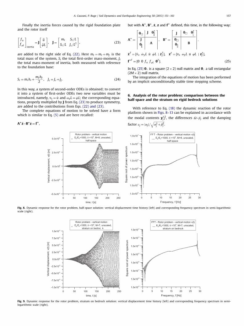
Fig. 8. Dynamic response for the rotor problem, half-space solution: vertical displacemscale (right).

Fig. 9. Dynamic response for the rotor problem, stratum on bedrock solution: verticallogarithmic scale (right).

but with A⋆, B⋆, _z, z and f⋆ defined, this time, in the following way:

_zT ¼ ½ _vx _ωyL _u _φL j _zTf �, zT ¼ ½vx ωyL u φL j zTf �,

f⋆T ¼ ½0 0 f u f φL 0T �: ð25Þ

In Eq. (25) 0□ is a square (2�2) null matrix and 0U a tall rectangular(2M�2) null matrix.

The integration of the equations of motion has been performedby an implicit unconditionally stable time stepping scheme.

6. Analysis of the rotor problem: comparison between thehalf-space and the stratum on rigid bedrock solutions

With reference to Eq. (18) the dynamic reaction of the rotorplatform shown in Figs. 8–13 can be explained in accordance with

the modal contents yTj f , the differences Ω−βj and the damping

factor νj ¼ jαjj=ffiffiffiffiffiffiffiffiffiffiffiffiffiffiffiα2j þβ2j

q.

ent time history (left) and corresponding frequency spectrum in semi-logarithmic

displacement time history (left) and corresponding frequency spectrum in semi-

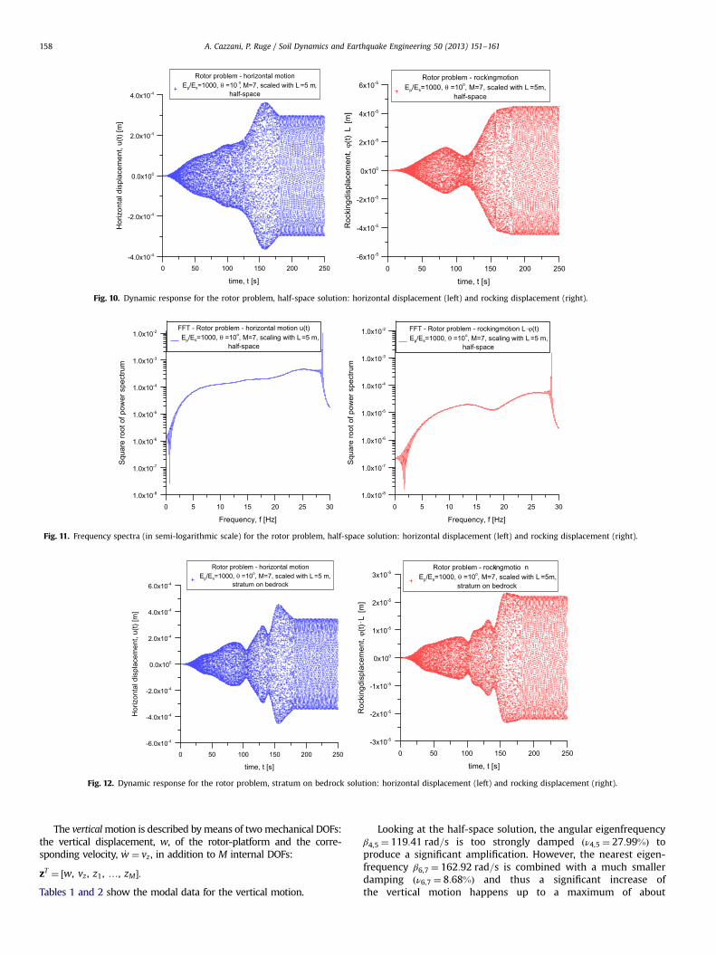
Fig. 10. Dynamic response for the rotor problem, half-space solution: horizontal displacement (left) and rocking displacement (right).

Fig. 11. Frequency spectra (in semi-logarithmic scale) for the rotor problem, half-space solution: horizontal displacement (left) and rocking displacement (right).

Fig. 12. Dynamic response for the rotor problem, stratum on bedrock solution: horizontal displacement (left) and rocking displacement (right).


The verticalmotion is described bymeans of twomechanical DOFs:the vertical displacement, w, of the rotor-platform and the corre-sponding velocity, _w ¼ vz , in addition to M internal DOFs:

zT ¼ ½w, vz , z1, …, zM�:Tables 1 and 2 show the modal data for the vertical motion.

Looking at the half-space solution, the angular eigenfrequencyβ4,5 ¼ 119:41 rad=s is too strongly damped ðν4,5 ¼ 27:99%Þ toproduce a significant amplification. However, the nearest eigen-frequency β6,7 ¼ 162:92 rad=s is combined with a much smallerdamping ðν6,7 ¼ 8:68%Þ and thus a significant increase ofthe vertical motion happens up to a maximum of about

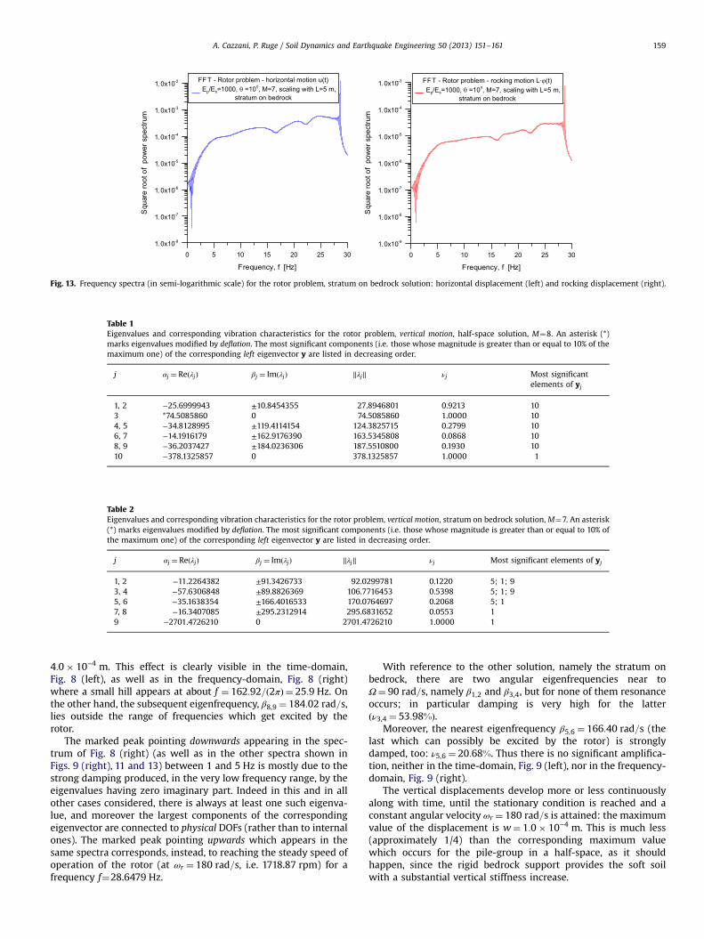
Fig. 13. Frequency spectra (in semi-logarithmic scale) for the rotor problem, stratum on bedrock solution: horizontal displacement (left) and rocking displacement (right).

Table 1Eigenvalues and corresponding vibration characteristics for the rotor problem, vertical motion, half-space solution, M¼8. An asterisk (*)marks eigenvalues modified by deflation. The most significant components (i.e. those whose magnitude is greater than or equal to 10% of themaximum one) of the corresponding left eigenvector y are listed in decreasing order.

j αj ¼ ReðλjÞ βj ¼ ImðλjÞ ∥λj∥ νj Most significantelements of yj

1, 2 −25.6999943 ±10.8454355 27.8946801 0.9213 103 *74.5085860 0 74.5085860 1.0000 104, 5 −34.8128995 ±119.4114154 124.3825715 0.2799 106, 7 −14.1916179 ±162.9176390 163.5345808 0.0868 108, 9 −36.2037427 ±184.0236306 187.5510800 0.1930 1010 −378.1325857 0 378.1325857 1.0000 1

Table 2Eigenvalues and corresponding vibration characteristics for the rotor problem, vertical motion, stratum on bedrock solution, M¼7. An asterisk(*) marks eigenvalues modified by deflation. The most significant components (i.e. those whose magnitude is greater than or equal to 10% ofthe maximum one) of the corresponding left eigenvector y are listed in decreasing order.

j αj ¼ ReðλjÞ βj ¼ ImðλjÞ ∥λj∥ νj Most significant elements of yj

1, 2 −11.2264382 ±91.3426733 92.0299781 0.1220 5; 1; 93, 4 −57.6306848 ±89.8826369 106.7716453 0.5398 5; 1; 95, 6 −35.1638354 ±166.4016533 170.0764697 0.2068 5; 17, 8 −16.3407085 ±295.2312914 295.6831652 0.0553 19 −2701.4726210 0 2701.4726210 1.0000 1


4:0� 10−4 m. This effect is clearly visible in the time-domain,Fig. 8 (left), as well as in the frequency-domain, Fig. 8 (right)where a small hill appears at about f ¼ 162:92=ð2πÞ ¼ 25:9 Hz. Onthe other hand, the subsequent eigenfrequency, β8,9 ¼ 184:02 rad=s,lies outside the range of frequencies which get excited by therotor.

The marked peak pointing downwards appearing in the spec-trum of Fig. 8 (right) (as well as in the other spectra shown inFigs. 9 (right), 11 and 13) between 1 and 5 Hz is mostly due to thestrong damping produced, in the very low frequency range, by theeigenvalues having zero imaginary part. Indeed in this and in allother cases considered, there is always at least one such eigenva-lue, and moreover the largest components of the correspondingeigenvector are connected to physical DOFs (rather than to internalones). The marked peak pointing upwards which appears in thesame spectra corresponds, instead, to reaching the steady speed ofoperation of the rotor (at ωr ¼ 180 rad=s, i.e. 1718.87 rpm) for afrequency f¼28.6479 Hz.

With reference to the other solution, namely the stratum onbedrock, there are two angular eigenfrequencies near toΩ¼ 90 rad=s, namely β1,2 and β3,4, but for none of them resonanceoccurs; in particular damping is very high for the latterðν3,4 ¼ 53:98%Þ.

Moreover, the nearest eigenfrequency β5,6 ¼ 166:40 rad=s (thelast which can possibly be excited by the rotor) is stronglydamped, too: ν5,6 ¼ 20:68%. Thus there is no significant amplifica-tion, neither in the time-domain, Fig. 9 (left), nor in the frequency-domain, Fig. 9 (right).

The vertical displacements develop more or less continuouslyalong with time, until the stationary condition is reached and aconstant angular velocity ωr ¼ 180 rad=s is attained: the maximumvalue of the displacement is w¼ 1:0� 10−4 m. This is much less(approximately 1/4) than the corresponding maximum valuewhich occurs for the pile-group in a half-space, as it shouldhappen, since the rigid bedrock support provides the soft soilwith a substantial vertical stiffness increase.

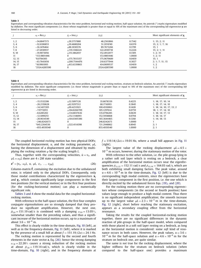
Table 3Eigenvalues and corresponding vibration characteristics for the rotor problem, horizontal and rocking motions, half-space solution. An asterisk (*) marks eigenvalues modifiedby deflation. The most significant components (i.e. those whose magnitude is greater than or equal to 10% of the maximum one) of the corresponding left eigenvector y arelisted in decreasing order.


1, 2 −34.8847575 ±30.3757880 46.2561866 0.7542 1; 15; 2; 113, 4 −32.6106853 ±39.4680204 51.1974749 0.6370 15; 2; 1; 7; 165, 6 −16.1476464 ±88.3030376 89.7673266 0.1799 15; 17, 8 −27.2030937 ±119.1368224 122.2030718 0.2226 15; 2; 1; 119, 10 −19.9073056 ±151.1862017 152.4912077 0.1305 1; 2; 1511 *153.9801446 0 153.9801446 1.0000 1; 2; 1112, 13 *8.0784305 ±175.7815357 175.9670689 0.0459 15; 114, 15 −63.7643656 ±200.7544476 210.6377044 0.3027 2; 1; 7; 11; 1516, 17 *18.9961005 ±413.6339865 414.0699537 0.0459 1; 218 *2524.4285590 0 2524.4285590 1.0000 1; 2

Table 4Eigenvalues and corresponding vibration characteristics for the rotor problem, horizontal and rocking motions, stratum on bedrock solution. An asterisk (*) marks eigenvaluesmodified by deflation. The most significant components (i.e. those whose magnitude is greater than or equal to 10% of the maximum one) of the corresponding lefteigenvector y are listed in decreasing order.


1, 2 −15.1532206 ±32.5097126 35.8678339 0.4225 1; 18; 17; 10; 143, 4 −26.2150628 ±62.9297312 68.1716993 0.3845 1; 18; 17; 14; 105, 6 −14.3457205 ±99.4253921 100.4550063 0.1428 1; 18; 14; 10; 17; 13; 27, 8 −7.9772055 ±104.8266709 105.1297614 0.0759 18; 1; 17; 14; 109, 10 −8.6285202 ±134.8037636 135.0796285 0.0639 1; 18; 14; 17; 1311, 12 −12.1099251 ±152.1146093 152.5958868 0.0794 1; 18; 14; 1713, 14 −20.9614549 ±164.0305386 165.3644465 0.1268 1; 14; 18; 1315 −246.8242673 0 246.8242673 1.0000 116, 17 *645.2264536 ±322.4114398 721.2948862 0.8945 2; 118 −855.4939540 0 855.4939540 1.0000 2; 1


The coupled horizontal-rocking motion has two physical DOFs;the horizontal displacement, u, and the rocking parameter, φL,having the dimension of a displacement and obtained by multi-plying the rocking rotation φ by the scaling length L.

Thus, together with the corresponding velocities, _u ¼ vx, and_φL¼ ωyL there are 4þ2M state variables:

zT ¼ ½vx, ωyL, u, φL, z1, …, z2M �: ð26ÞColumn-matrix f , containing the excitation due to the unbalancedrotor, is related only to the physical DOFs. Consequently, onlythose modal contributions characterized by the eigenvectors xj

and yj, which contain significantly large components in the firsttwo positions (for the vertical motion) or in the first four positions(for the rocking-horizontal motion) can play a numericallysignificant role.

Tables 3 and 4 show the modal data for the coupled horizontal-rocking motion.

With reference to the half-space solution, the first four complexconjugate eigensolutions are so strongly damped that they pro-duce no significant amplification. However, the next one,β5,6 ¼ 151:19 rad=s is combined with a damping ν5,6 ¼ 13:05%,somewhat smaller than the preceding values, and thus a signifi-cant increase of the horizontal motion occurs, up to a maximum ofabout 3:6� 10−4 m.

This effect is clearly visible in the time-domain, Fig. 10 (left), aswell as in the frequency-domain, Fig. 11 (left), where it is markedby the presence of a small hill at about f ¼ 151:19=ð2πÞ ¼ 24:1 Hz.

The rocking motion is represented by the second and fourthelements in the state vector z, Eq. (26): hence the strong dampingν7,8 ¼ 22:26% causes a strong reduction of the rocking motionat about β7,8 ¼ 119:14 rad=s, which is clearly visible in thetime-domain, Fig. 10 (right), and in the frequency domain at

f ¼ 119:14=ð2πÞ ¼ 19:01 Hz, where a small hill appears in Fig. 11(right).

The largest value of the rocking displacement φL¼ 4:5�10−5 m occurs, however, during the stationary motion of the rotor.

With reference to the other solution, i.e. the pile-group lying ina rather soft soil layer which is resting on a bedrock, a clearamplification of the horizontal motion occurs near the eigenfre-quencies β11,12 ¼ 152:11 rad=s and β13,14 ¼ 164:03 rad=s, which areboth exhibiting small damping factors. The peak value, aroundu¼ 4:6� 10−4 m in the time-domain, Fig. 12 (left) is due to thecorresponding high modal contents, since the eigenvectors havetheir largest component in the first position, i.e. the one which isdirectly excited by the unbalanced forces Eqs. (19)1 and (20).

For the rocking motion there are no corresponding eigenvec-tors whose components (in the second or fourth position) havevalues large enough to produce a high modal content. Thus thereis no significant independent amplification; the smooth increaseup to the largest value φL¼ 2:3� 10−5 m in the time-domain,Fig. 12 (right), short before reaching the stationary excitation,appears as a secondary coupling effect from the horizontalresonance.

Taking the results for the coupled horizontal-rocking motiontogether, there are no significant differences in the dynamicreaction of pile-groups in the half-space model, when comparedwith those placed in a soft soil layer resting on a bedrock, as longas the horizontal motion is considered: some soft kind of reso-nance occurs in both cases. However, the peak values, u¼ 3:6�10−4 m for the half-space solution and u¼ 4:6� 10−4 m for thestratum on bedrock one, are quite similar.

The same is not true for the rocking displacement, where thehigher stiffness for the stratum on bedrock solution (whencompared to the half-space one) provides a maximum


displacement value which is almost halved: indeedφL¼ 2:3� 10−5 m, in the former case, while φL¼ 4:5� 10−5 m, inthe latter.

7. Numerical robustness of the dynamic system

Contributions to the numerical solution of wave propagationproblems by means of polynomial representations based on a BEMapproach or on a SBFEM procedure clearly mention the appear-ance of spurious modes.

Some advance in this issue has been obtained by the use ofscaling; either by scaling the DOF-related quantities, in such a waythat they are represented by common physical dimensions [2]; orby a more general concept recently published by Birk et al., see[13].

Nevertheless, remaining spurious modes characterized byeigenvalues λk ¼ αkþ iβk with positive real part can be forcedlycast into the left part of the complex plane by spectral shifting,while maintaining the full modal space. The influence of the shifthas been identified in [2] and can be optimized.

By comparing the modal data, the eigenvectors and eigenva-lues, before and after this so-called deflation process, typicallyshow an excellent agreement: the first 8 digits of the componentsof the eigenvectors are identical and, for the eigenvalues, an evenbetter matching is achieved.

However in particular conditions, which cannot be a prioriidentified yet, the deflation procedure fails and instability occurs:this happened, for instance, when treating the vertical motion inthe half-space solution with the choice of M¼7 as the order of thePadé approximation. Surprisingly, by changing fromM¼7 toM¼5,M¼6 or, even, M¼8 or M¼9 stable results were recovered, as ithappened for all other cases presented in this paper. The results ofthe vertical motion for the half-space solution presented here, inTable 1 and in Fig. 10, are those relevant to the choice M¼8.

A deeper understanding of the above-mentioned failure of thedeflation procedure goes beyond the scope of this work, and willbe the subject of a forthcoming paper.

8. Conclusions

Nowadays it is a well-accepted evidence that the contributionof the soil to the dynamics of the whole soil–structure system isfrequency-dependent. This influence remains true even for thecase of a pile foundation, where inclined pile-groups fitted into thesoil have been studied by Padrón et al. [1] in two differentscenarios: as an unbounded half-space medium and as a horizon-tally unbounded, fixed thickness layer resting on a rigid bedrock,where additional layer resonance frequencies can appear.

For a typical rotor platform on pile groups running throughresonance it has been shown in this paper that a rational inter-polation is able to approximate (even in the case of end-bearingpile-groups) a given set of complex stiffness data.

It is found that the additional layer-frequencies which areexpected in the case of a soil stratum of finite thickness lyingabove a rigid bedrock do not cause additional peaks in the reactionof the foundation slab, because the corresponding damping due tothe soil is strong enough to significantly suppress these peaks.

As a final closing, it is apparent that in passing throughresonance points there are no strong differences, in the average,from an engineering point of view, between the dynamic reactionof pile-groups in half-space compared to pile-groups placed abovea soil stratum resting on a bedrock.

Acknowledgments

A grant to P. Ruge covering a three-month stay in Cagliari wasprovided by RAS (the Autonomous Region of Sardinia) under theVisiting Professor Programme for Academic Year 2011–2012; thisfinancial support is gratefully acknowledged, as well as thatprovided to A. Cazzani by the University of Cagliari for Year 2011.

Special thanks to Prof. L.A. Padrón, corresponding author, forkindly providing the original data used to draw Figs. 15–18 ofpaper [1], along with useful directions for treating them. His helpand prompt cooperative effort are gratefully acknowledged.

Finally the authors want to express particular thanks to F.Stochino for his professional help in producing one of the figures.

References

[1] Padrón LA, Aznárez JJ, Maeso O, Saitoh M. Impedance functions of end-bearinginclined piles. Soil Dynamics and Earthquake Engineering 2012;38:97–108.

[2] Cazzani A, Ruge P. Numerical aspects of coupling strongly frequency-dependent soil–foundation models with structural finite elements in thetime-domain. Soil Dynamics and Earthquake Engineering 2012;37:56–72.

[3] Jenck O, Dias D, Kastner R. Three-dimensional numerical modeling of a piledembankment. International Journal of Geomechanics 2009;9:102–12.

[4] Lehmann L. Wave propagation in infinite domains. Berlin, Heidelberg, NewYork: Springer Verlag; 2007.

[5] Lai WL, Rubin D, Krempl E. Introduction to continuum mechanics. 3rd ed.Woburn, MA: Butterworth Heinemann; 1999.

[6] Ruge P, Trinks C, Witte S. Time-domain analysis of unbounded media usingmixed-variable formulations. Earthquake Engineering and StructuralDynamics 2001;30:899–925.

[7] Ruge P, Zulkifli E, Birk C. Symmetric matrix-valued frequency to timetransformation for unbounded domains applied to infinite beams. Computersand Structures 2006;84:1815–26.

[8] Trinks C. Consistent absorbing boundaries for time-domain interaction ana-lyses using the fractional calculus. PhD thesis; Technische Universität Dresden;2004.

[9] Zulkifli E. Consistent description of radiation damping in transient soil–structure interaction. PhD thesis; Technische Universität Dresden; 2008.

[10] Padrón LA, Aznárez JJ, Maeso O, Santana A. Dynamic stiffness of deepfoundations with inclined piles. Earthquake Engineering and StructuralDynamics 2010;39:1343–67.

[11] Clough RW, Penzien J. Dynamics of structures. New York: McGraw-Hill; 1975.[12] Markert R, Seidler M. Analytically based estimation of the maximum ampli-

tude during passage through resonance. International Journal of Solids andStructures 2001;38:1975–92.

[13] Birk C, Prempramote S, Song C. An improved continued-fraction-based high-order transmitting boundary for time-domain analyses in unboundeddomains. International Journal for Numerical Methods in Engineering2012;89:269–98.

rotor platforms on pile-groups running through resonance: a comparison between unbounded soil and...

Documents