role of trade, external debt, labor force and education in economic growth
TRANSCRIPT
European Journal of Scientific Research
ISSN: 1450-216X Volume 20, No 4 July, 2008 Editor-In-chief or e Adrian M. Steinberg, Wissenschaftlicher Forscher Editorial Advisory Board e Parag Garhyan, Auburn University Morteza Shahbazi, Edinburgh University Raj Rajagopalan, National University of Singapore Sang-Eon Park, Inha University Said Elnashaie, Auburn University Subrata Chowdhury, University of Rhode Island Ghasem-Ali Omrani, Tehran University of Medical Sciences Ajay K. Ray, National University of Singapore Mutwakil Nafi, China University of Geosciences Felix Ayadi, Texas Southern University Bansi Sawhney, University of Baltimore David Wang, Hsuan Chuang University Cornelis A. Los, Kazakh-British Technical University Jatin Pancholi, Middlesex University
Teresa Smith, University of South Carolina Ranjit Biswas, Philadelphia University Chiaku Chukwuogor-Ndu, Eastern Connecticut State University John Mylonakis, Hellenic Open University (Tutor) M. Femi Ayadi, University of Houston-Clear Lake Emmanuel Anoruo, Coppin State University H. Young Baek, Nova Southeastern University Dimitrios Mavridis, Technological Educational Institure of West Macedonia Mohand-Said Oukil, Kind Fhad University of Petroleum & Minerals Jean-Luc Grosso, University of South Carolina Richard Omotoye, Virginia State University Mahdi Hadi, Kuwait University Jerry Kolo, Florida Atlantic University Leo V. Ryan, DePaul University
As of 2005, European Journal of Scientific Research is indexed in ULRICH, DOAJ and CABELL academic listings.

European Journal of Scientific Research http://www.eurojournals.com/ejsr.htm Editorial Policies: 1) European Journal of Scientific Research is an international official journal publishing high quality research papers, reviews, and short communications in the fields of biology, chemistry, physics, environmental sciences, mathematics, geology, engineering, computer science, social sciences, medicine, industrial, and all other applied and theoretical sciences. The journal welcomes submission of articles through [email protected]. 2) The journal realizes the meaning of fast publication to researchers, particularly to those working in competitive & dynamic fields. Hence, it offers an exceptionally fast publication schedule including prompt peer-review by the experts in the field and immediate publication upon acceptance. It is the major editorial policy to review the submitted articles as fast as possible and promptly include them in the forthcoming issues should they pass the evaluation process.
3) All research and reviews published in the journal have been fully peer-reviewed by two, and in some cases, three internal or external reviewers. Unless they are out of scope for the journal, or are of an unacceptably low standard of presentation, submitted articles will be sent to peer reviewers. They will generally be reviewed by two experts with the aim of reaching a first decision within a three day period. Reviewers have to sign their reports and are asked to declare any competing interests. Any suggested external peer reviewers should not have published with any of the authors of the manuscript within the past five years and should not be members of the same research institution. Suggested reviewers will be considered alongside potential reviewers identified by their publication record or recommended by Editorial Board members. Reviewers are asked whether the manuscript is scientifically sound and coherent, how interesting it is and whether the quality of the writing is acceptable. Where possible, the final decision is made on the basis that the peer reviewers are in accordance with one another, or that at least there is no strong dissenting view.
4) In cases where there is strong disagreement either among peer reviewers or between the authors and peer reviewers, advice is sought from a member of the journal's Editorial Board. The journal allows a maximum of two revisions of any manuscripts. The ultimate responsibility for any decision lies with the Editor-in-Chief. Reviewers are also asked to indicate which articles they consider to be especially interesting or significant. These articles may be given greater prominence and greater external publicity.
5) Any manuscript submitted to the journals must not already have been published in another journal or be under consideration by any other journal, although it may have been deposited on a preprint server. Manuscripts that are derived from papers presented at conferences can be submitted even if they have been published as part of the conference proceedings in a peer reviewed journal. Authors are required to ensure that no material submitted as part of a manuscript infringes existing copyrights, or the rights of a third party. Contributing authors retain copyright to their work.
6) Submission of a manuscript to EuroJournals, Inc. implies that all authors have read and agreed to its content, and that any experimental research that is reported in the manuscript has been performed with the approval of an appropriate ethics committee. Research carried out on humans must be in compliance with the Helsinki Declaration, and any experimental research on animals should follow internationally recognized guidelines. A statement to this effect must appear in the Methods section of the manuscript, including the name of the body which gave approval, with a reference number where

appropriate. Manuscripts may be rejected if the editorial office considers that the research has not been carried out within an ethical framework, e.g. if the severity of the experimental procedure is not justified by the value of the knowledge gained. Generic drug names should generally be used where appropriate. When proprietary brands are used in research, include the brand names in parentheses in the Methods section.
7) Manuscripts must be submitted by one of the authors of the manuscript, and should not be submitted by anyone on their behalf. The submitting author takes responsibility for the article during submission and peer review. To facilitate rapid publication and to minimize administrative costs, the journal accepts only online submissions through [email protected]. E-mails should clearly state the name of the article as well as full names and e-mail addresses of all the contributing authors.
8) The journal makes all published original research immediately accessible through www.EuroJournals.com without subscription charges or registration barriers. European Journal of Scientific Research indexed in ULRICH, DOAJ and CABELL academic listings. Through its open access policy, the Journal is committed permanently to maintaining this policy. All research published in the. Journal is fully peer reviewed. This process is streamlined thanks to a user-friendly, web-based system for submission and for referees to view manuscripts and return their reviews. The journal does not have page charges, color figure charges or submission fees. However, there is an article-processing and publication charge. Further information is available at: http://www.eurojournals.com/ejsr.htm © EuroJournals Publishing, Inc. 2005

European Journal of Scientific Research Volume 20, No 4 May 2008
Contents Blast-Hole Cuttings: An Indicator of Drill Bit Wear in Quarries 721-736 Z.O. Opafunso and B. Adebayo Assessment of Micro-Credit Supply by Country Women Association of Nigeria (Cowan) to Rural Women in Ondo State, Nigeria 737-745 M.G. Olujide Comparative Analysis of Pictorial Coverage of Events by Pakistan’s English Press 746-758 Muhammad Nawaz Mahsud, Muhammad Khalid and Firasat Jabeen Design Space Exploration of Regular NoC Architectures: A Multi-Objective Evolutionary Algorithm Approach 759-771 Rabindra Ku. Jena, Musbah M. Aqel, Gopal K. Sharma and Prabhat K. Mahanti Etude Comparative des Méthodes D’évaluation de la Vulnérabilité à la Pollution des Aquifères en Milieu Poreux: Application Aux Eaux Souterraines du District D’abidjan (Sud de la Côte D’ivoire) 772-787 Kouamé Kan Jean, Jourda Jean Patrice, Adja Miessan Germain Deh Serges Kouakou, Anani Abenan Tawa, Effini Adiow Thérèse and Biémi Jean Development of an Interated Poultry/Fishery Husbandry for Optimal Agricultural Production 788-795 F.R. Falayi, A.S. Ogunlowo and M.O. Alatise Robust Control of a Doubly Fed Asynchronous Machine of a Wind Turbine System 796-804 S. Gherbi, S. Yahmedi and M. Sedraoui Effects of Enviromental Variables on Poultry Performance and Pond Water Quality in an Integrated Poultry/Fishery Farming 805-816 F.R. Falayi, A.S. Ogunlowo and M.O. Alatise Spatial Distribution and Characterisation of the Sediments of the Estuary of Comoe River (Grand-Bassam, Côte D’ivoire) 817-827 Adopo Kouassi Laurent, Kouassi Kouakou Lazare, Wognin Ama Valérie Irma Monde Sylvain, Meledje N’Diaye Hermann and Aka Kouamé Blind SIMO GSM Channel Identification 828-835 Taba Mohamed Tahar, S. Femmame and D. Mossadeg The Chemical Control of the Pests in the Truck Farming and the Quality of Vegetables in African Urban Cities: The Health Hazards and Security of Consumers 836-843 Dembele Ardjouma, Oumarou Badini, Traore Sory Karim, Mamadou Koné Coulibaly D. Ténébé and A. Abba Toure

Database Interfacing using Natural Language Processing 844-851 Imran Sarwar Bajwa, Shahzad Mumtaz and M. Shahid Naweed Role of Trade, External Debt, Labor Force and Education in Economic Growth Empirical Evidence from Pakistan by using ARDL Approach 852-862 Arshad Hasan and Safdar Butt Development of Mechanical Prosthetic Hand System for BCI Application 863-870 N. A Abu Osman, S. Yahud and S. Y Goh Toxicity of Arsenic in the Ground Water of Comarca-Lagunera (Mexico) 871-881 Faten Semadi, Vincent Valles and Jose Luis Gonzalez Barrios Modeling and Temperature Controller Design for Yazd Solar Power Plant 882-890 Aref Shahmansoorian and Abdolvahed Saidi A Predictive Current Control Technique on Fuel Cell Based Distributed Generation in a Standalone AC Power Supply 891-904 K. G. Firouzjah, H. Eshaghtabar, A. Sheikholeslami and S. Lesan Effects of Ethyl acetate Portion of Syzygium Aromaticum Flower Bud Extract on Indomethacin-Induced Gastric Ulceration and Gastric Secretion 905-913 Okasha Mohammad Abdul- Halim, Magaji Rabiu Abdussalam Abubakar Mujtaba Suleiman and Fatihu Muhammad Yakasai Real Digital TV Accessed by Cellular Mobile System 914-923 Basil M. Kasasbeh, Rafa E. Al-Qutaish, Muzhir S. Al-Ani and Khalid Al-Sarayreh A Rule-Based Fuzzy Automatic Voltage Regulator for Power System Stability 924-933 Samuel N. Ndubisi and Marcel .U. Agu

European Journal of Scientific Research ISSN 1450-216X Vol.20 No.4 (2008), pp.721-736 © EuroJournals Publishing, Inc. 2008 http://www.eurojournals.com/ejsr.htm
Blast-Hole Cuttings: An Indicator of Drill Bit Wear in Quarries
Z.O. Opafunso Department of Mining Engineering, Federal University of Technology
Akure, NIGERIA
B. Adebayo Department of Mining Engineering, Federal University of Technology
Akure, NIGERIA
Abstract
This paper deals with the evaluation of blast-hole cuttings generated in process creating cavity in a rock mass as an indicator of bit wear. Blast-hole cuttings were collected on each hole drilled until drill bit is worn completely and deterioration of button inserted on the surface of the bit was measured as well. The size distribution of the blast-hole cuttings collected from the three selected quarries in South Western Nigeria was determined using sieve shaker. The results obtained show that weight retained on 850µm decreases while weight of blast-hole cuttings retained on 75 µm increases. The regression carried out gives values R² = 0.957, R² = 0.777, and R² = 0.729 for Geovertrag Quarry, Ado-Ekiti, Johnson Quarry, Akure and Sonel Boneh Quarry, Ibadan respectively. This shows that there is strong relationship between gauge button wear rate and weight of blast-hole cuttings retained on 75 µm sieve size. Therefore, monitoring the blast-hole cuttings while drilling could help to ascertained worn drill bit in a quarry.
Introduction Rock penetration is the process by which ‘bit’ the applicator of energy advance into the rock in response to drill tool power as well as thrust. Howarth et al (1986) carried out percussion drilling test on ten sedimentary and crystalline rocks. Therefore, drilling is the process of creating artificial cavity in a rock mass for the purpose of placement of explosives. Studies have shown that assessing drilling mechanisms, it is a fact that besides compressive and tensile (percussive process) and shear strength (bit rotation) the elastic characteristics of rock material is crucial.
However, blast-hole cuttings are produced in the course of rock drill bit advancing into the rock mass. Thuro (1997) summarized crushing process leading to the production of blast-hole cuttings under the buttons of a drill bit; around the contact of the button a new state of stress is induced in the rock, where four important destruction mechanisms can be distinguished: under the bit button a crushed zone of fine rock powder is formed (impact), starting from the from the crushed powdered zone, radial cracks are developed (induced tensile stress) when stress the rock is high enough large fragments of the rock can be sheared off between the button grooves (shear stress) and added to the mechanisms above stress is induced periodically (dynamic process).
Chiang and Elias (2000) identified that the impact frequency rate, the workings of air pressure, the thrust force and rotation torque are important in the generation of blast-hole cuttings. The last two parameters are estimated by reading the impact pressure to the hydraulic motor or hydraulic cylinder respectively. The brittleness which is defined as lack of ductility can aid fracture failure and formation

Blast-Hole Cuttings: An Indicator of Drill Bit Wear in Quarries 722
of fines (Morley, 1944 and Hetenyi, 1966). Blast-hole cuttings are debris, chippings or caving flushed by compressed air rock is attacked mechanically.
In addition, to effectively remove the blast-hole cuttings, annular space should be about 17% of the cross-sectional area of the blast-hole. If the percentage of the annular space is less than 17% then for every 1% reduction in this percentage the bailing velocity must be increased by 2% (Gokhale, 2004). An estimated correlation factor on account of insufficient annular space is given as:
aa = (1+ 0.02) [17-A] (1) Where A is the percentage of annular space for combination of bit and drill rods to be used in
actual drilling (if A is more than 17% then aa should be given a value 1). Beste (2004) observed that it is difficult to get an overview of wear mechanisms of the rock
drill bit. Shah and Wong (1997) were of the view that the contact geometry between tungsten-carbide insert and rock is complex. Wear of rock drill bit is a constant phenomenon in hard rock drilling which cannot be avoided; this may be a severe factor of cost for effective management of quarries, hence, a reasonable measurement and prediction would be desirable. Moreover, when the drilling time increases as well as low penetration rate, one can infer that the button of the bit is likely to be dull or worn and of course this can lead to regrinding of blast-hole cuttings.
Therefore, utilization of energy to achieve penetration, under normal condition depends on drillability of the rock; a certain amount of energy will be dissipated by rock breakage. It was discovered through research that when bit button is blunt after very few impacts the hammer will become useless because of plastic deformation. The bit which has the shortest span of all the three main components will last in the order of 120 million cycles and the main cause of the failure is wear (Chiang and Elias, 2000) and as the bit buttons wear out more fines are likely to be generated. The objective of this paper therefore, are to use blast-hole cuttings as a measure of bit wear rate as well correlate the weight retained at 75µm sieve size in order to establish their relationship. Materials and Method The materials for this work includes: blast-hole cuttings collected from 45 holes from three Nigeria quarries and drill bit Method
The grain size of 45 blast-holes drill cuttings collected from three selected quarries were determined using standard method of America Society for Testing and Materials (ASTM) D 2487 and sieve of the following mesh sizes: 850 µm, 600µm, 425µm, 300µm, 212µm, 150µm, 75µm, and 63µm were used the results are presented in Table 1-45 and The wear of the gauge buttons were measured at regular interval this correlated with weight retained on 75µm sieve size. Result and Discussion Tables 1-46 present the size distribution of the blast-hole cutting, it is observe that as number of hole drill and wear increases the weight blast-hole cuttings retained on 850 µm decreases the weight of blast-hole cuttings retained on the 75µm sieve size increases. All these point to the fact that it is likely that as bit button is blunt, regrinding of blast-hole occurs.
Figure 1 shows the correlation between bit gauge button wear rate and weight of blast-hole cuttings retained on 75µm sieve size cuttings from Geovertrag Quarry, Ado-Ekiti. The polynomial relationship between Gauge button wear rate and weight of blast-hole cuttings retained on 75µm sieve size is expressed by equation 2 which is an equation of order 2 and R2 = 0.957.
Gw = -3E-05wt2 + 0.003x - 0.099, R² = 0.957 (2) Where Gw is gauge wear rate and wt is the weight of blast-hole cuttings retained on 75µm
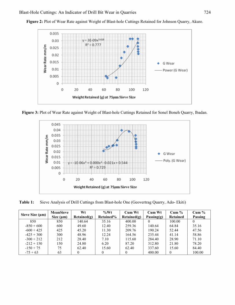
sieve size. Figure 2 presents the correlation between bit gauge button wear rate and weight of blast-
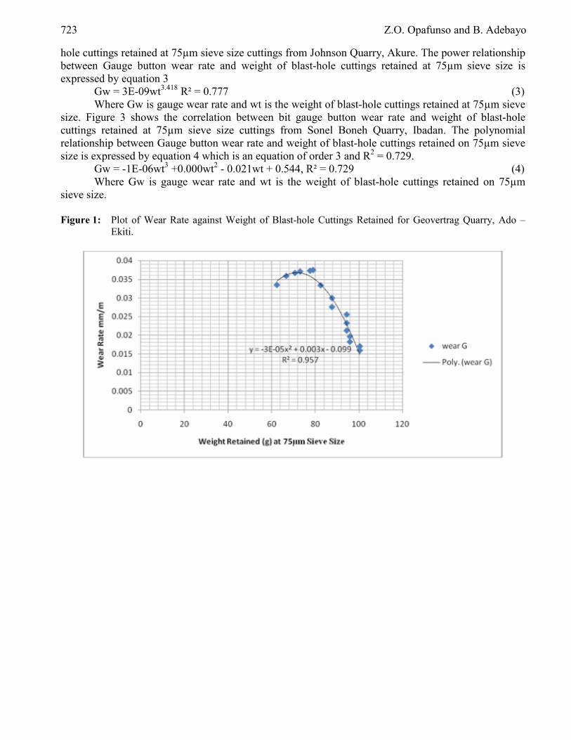
723 Z.O. Opafunso and B. Adebayo
hole cuttings retained at 75µm sieve size cuttings from Johnson Quarry, Akure. The power relationship between Gauge button wear rate and weight of blast-hole cuttings retained at 75µm sieve size is expressed by equation 3
Gw = 3E-09wt3.418 R² = 0.777 (3) Where Gw is gauge wear rate and wt is the weight of blast-hole cuttings retained at 75µm sieve
size. Figure 3 shows the correlation between bit gauge button wear rate and weight of blast-hole cuttings retained at 75µm sieve size cuttings from Sonel Boneh Quarry, Ibadan. The polynomial relationship between Gauge button wear rate and weight of blast-hole cuttings retained on 75µm sieve size is expressed by equation 4 which is an equation of order 3 and R2 = 0.729.
Gw = -1E-06wt3 +0.000wt2 - 0.021wt + 0.544, R² = 0.729 (4) Where Gw is gauge wear rate and wt is the weight of blast-hole cuttings retained on 75µm
sieve size. Figure 1: Plot of Wear Rate against Weight of Blast-hole Cuttings Retained for Geovertrag Quarry, Ado –
Ekiti.
Blast-Hole Cuttings: An Indicator of Drill Bit Wear in Quarries 724
Figure 2: Plot of Wear Rate against Weight of Blast-hole Cuttings Retained for Johnson Quarry, Akure.
Figure 3: Plot of Wear Rate against Weight of Blast-hole Cuttings Retained for Sonel Boneh Quarry, Ibadan.
Table 1: Sieve Analysis of Drill Cuttings from Blast-hole One (Geovertrag Quarry, Ado- Ekiti) Sieve Size (µm) MeanSieve
Size (µm) Wt
Retained(g) %Wt
Retained% Cum Wt
Retained(g) Cum Wt
Passing(g) Cum % Retained
Cum % Passing
850 850 140.64 35.16 400.00 0 100.00 0 -850 + 600 600 49.60 12.40 259.36 140.64 64.84 35.16 -600 + 425 425 45.20 11.30 209.76 190.24 52.44 47.56 -425 + 300 300 48.96 12.24 164.56 235.44 41.14 58.86 -300 + 212 212 28.40 7.10 115.60 284.40 28.90 71.10 -212 + 150 150 24.80 6.20 87.20 312.80 21.80 78.20 -150 + 75 75 62.40 15.60 62.40 337.60 15.60 84.40 -75 + 63 63 0 0 0 400.00 0 100.00

725 Z.O. Opafunso and B. Adebayo
Table 2: Sieve Analysis of Drill Cuttings from Blast-hole Two (Govertrag Quarry, Ado- Ekiti) Sieve Size (µm) MeanSieve
Size (µm) Wt
Retained(g) %Wt
Retained% Cum Wt
Retained(g) Cum Wt
Passing(g) Cum % Retained
Cum % Passing
850 850 140.36 35.09 400.00 0 100.00 0 -850 + 600 600 45.60 11.40 259.64 140.36 64.91 35.09 -600 + 425 425 41.20 10.30 214.04 185.96 53.51 46.49 -425 + 300 300 44.96 11.24 172.84 227.16 43.21 56.79 -300 + 212 212 32.40 8.10 127.88 272.12 31.97 68.03 -212 + 150 150 28.80 7.20 95.48 304.52 23.87 76.13 -150 + 75 75 66.68 16.67 66.68 333.32 16.67 83.33 -75 + 63 63 0 0 0 400.00 0 100.00
Table 3: Sieve Analysis of Drill Cuttings from Blast-hole Three (Govertrag Quarry, Ado- Ekiti) Sieve Size (µm) MeanSieve
Size (µm) Wt
Retained(g) %Wt
Retained% Cum Wt
Retained(g) Cum Wt
Passing(g) Cum % Retained
Cum % Passing
850 850 140.36 35.09 400.00 0 100.00 0 -850 + 600 600 41.60 10.40 259.64 140.36 64.91 35.09 -600 + 425 425 37.20 9.30 218.04 181.96 54.51 45.49 -425 + 300 300 40.96 10.24 180.84 219.16 45.21 54.79 -300 + 212 212 36.40 9.10 139.88 260.12 34.97 65.03 -212 + 150 150 32.80 8.20 103.48 296.52 25.87 74.13 -150 + 75 75 70.68 17.67 70.68 329.32 17.67 82.33 -75 + 63 63 0 0 0 400.00 0 100.00
Table 4: Sieve Analysis of Drill Cuttings from Blast-hole Four (Govertrag Quarry, Ado- Ekiti)
Sieve Size (µm) MeanSieve Size (µm)
Wt Retained(g)
%Wt Retained%
Cum Wt Retained(g)
Cum Wt Passing(g)
Cum % Retained
Cum % Passing
850 850 138.00 34.50 400.00 0 100.00 0 -850 + 600 600 37.60 9.40 262.00 138.00 65.50 34.50 -600 + 425 425 33.20 8.30 224.40 175.00 56.10 43.90 -425 + 300 300 40.96 10.24 191.20 208.80 47.80 52.20 -300 + 212 212 40.40 10.10 150.24 249.76 37.56 62.44 -212 + 150 150 36.80 9.20 109.84 290.16 27.46 72.54 -150 + 75 75 73.04 18.26 73.04 326.96 18.26 81.74 -75 + 63 63 0 0 0 400.00 0 100.00
Table 5: Sieve Analysis of Drill Cuttings from Blast-hole Five (Govertrag Quarry, Ado- Ekiti)
Sieve Size (µm) MeanSieve Size (µm)
Wt Retained(g)
%Wt Retained%
Cum Wt Retained(g)
Cum Wt Passing(g)
Cum % Retained
Cum % Passing
850 850 128.00 32.00 399.99 0.01 99.99 0.01 -850 + 600 600 33.60 8.40 272.00 128.00 67.99 32.01 -600 + 425 425 32.40 8.10 238.40 161.62 59.59 40.41 -425 + 300 300 42.16 10.54 206.00 194.00 51.49 48.50 -300 + 212 212 44.26 11.06 163.84 236.68 40.95 59.05 -212 + 150 150 42.00 10.50 119.58 280.42 29.89 70.01 -150 + 75 75 77.58 19.39 77.59 322.40 19.39 80.60 -75 + 63 63 0 0 0.01 399.99 0.01 99.99
Blast-Hole Cuttings: An Indicator of Drill Bit Wear in Quarries 726
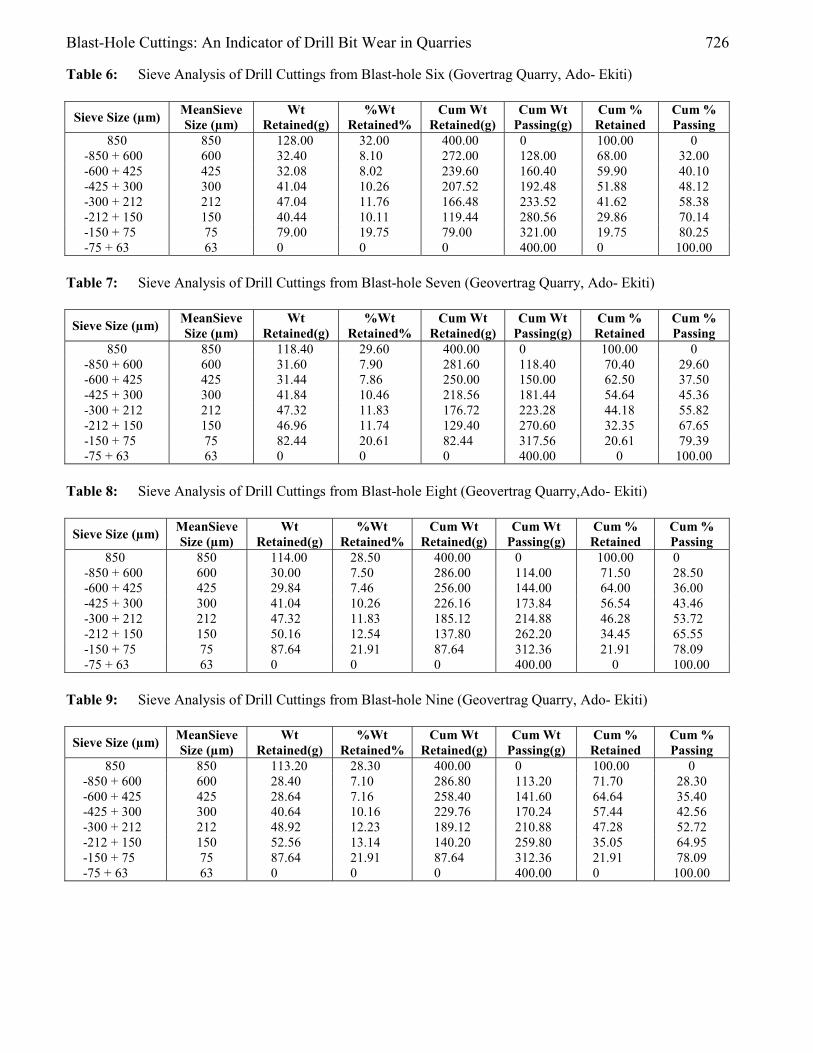
Table 6: Sieve Analysis of Drill Cuttings from Blast-hole Six (Govertrag Quarry, Ado- Ekiti)
Sieve Size (µm) MeanSieve Size (µm)
Wt Retained(g)
%Wt Retained%
Cum Wt Retained(g)
Cum Wt Passing(g)
Cum % Retained
Cum % Passing
850 850 128.00 32.00 400.00 0 100.00 0 -850 + 600 600 32.40 8.10 272.00 128.00 68.00 32.00 -600 + 425 425 32.08 8.02 239.60 160.40 59.90 40.10 -425 + 300 300 41.04 10.26 207.52 192.48 51.88 48.12 -300 + 212 212 47.04 11.76 166.48 233.52 41.62 58.38 -212 + 150 150 40.44 10.11 119.44 280.56 29.86 70.14 -150 + 75 75 79.00 19.75 79.00 321.00 19.75 80.25 -75 + 63 63 0 0 0 400.00 0 100.00
Table 7: Sieve Analysis of Drill Cuttings from Blast-hole Seven (Geovertrag Quarry, Ado- Ekiti) Sieve Size (µm) MeanSieve
Size (µm) Wt
Retained(g) %Wt
Retained% Cum Wt
Retained(g) Cum Wt
Passing(g) Cum % Retained
Cum % Passing
850 850 118.40 29.60 400.00 0 100.00 0 -850 + 600 600 31.60 7.90 281.60 118.40 70.40 29.60 -600 + 425 425 31.44 7.86 250.00 150.00 62.50 37.50 -425 + 300 300 41.84 10.46 218.56 181.44 54.64 45.36 -300 + 212 212 47.32 11.83 176.72 223.28 44.18 55.82 -212 + 150 150 46.96 11.74 129.40 270.60 32.35 67.65 -150 + 75 75 82.44 20.61 82.44 317.56 20.61 79.39 -75 + 63 63 0 0 0 400.00 0 100.00
Table 8: Sieve Analysis of Drill Cuttings from Blast-hole Eight (Geovertrag Quarry,Ado- Ekiti) Sieve Size (µm) MeanSieve
Size (µm) Wt
Retained(g) %Wt
Retained% Cum Wt
Retained(g) Cum Wt
Passing(g) Cum % Retained
Cum % Passing
850 850 114.00 28.50 400.00 0 100.00 0 -850 + 600 600 30.00 7.50 286.00 114.00 71.50 28.50 -600 + 425 425 29.84 7.46 256.00 144.00 64.00 36.00 -425 + 300 300 41.04 10.26 226.16 173.84 56.54 43.46 -300 + 212 212 47.32 11.83 185.12 214.88 46.28 53.72 -212 + 150 150 50.16 12.54 137.80 262.20 34.45 65.55 -150 + 75 75 87.64 21.91 87.64 312.36 21.91 78.09 -75 + 63 63 0 0 0 400.00 0 100.00
Table 9: Sieve Analysis of Drill Cuttings from Blast-hole Nine (Geovertrag Quarry, Ado- Ekiti) Sieve Size (µm) MeanSieve
Size (µm) Wt
Retained(g) %Wt
Retained% Cum Wt
Retained(g) Cum Wt
Passing(g) Cum % Retained
Cum % Passing
850 850 113.20 28.30 400.00 0 100.00 0 -850 + 600 600 28.40 7.10 286.80 113.20 71.70 28.30 -600 + 425 425 28.64 7.16 258.40 141.60 64.64 35.40 -425 + 300 300 40.64 10.16 229.76 170.24 57.44 42.56 -300 + 212 212 48.92 12.23 189.12 210.88 47.28 52.72 -212 + 150 150 52.56 13.14 140.20 259.80 35.05 64.95 -150 + 75 75 87.64 21.91 87.64 312.36 21.91 78.09 -75 + 63 63 0 0 0 400.00 0 100.00
727 Z.O. Opafunso and B. Adebayo
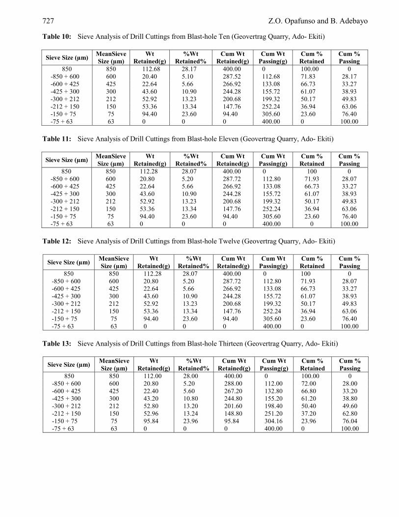
Table 10: Sieve Analysis of Drill Cuttings from Blast-hole Ten (Geovertrag Quarry, Ado- Ekiti)
Sieve Size (µm) MeanSieve Size (µm)
Wt Retained(g)
%Wt Retained%
Cum Wt Retained(g)
Cum Wt Passing(g)
Cum % Retained
Cum % Passing
850 850 112.68 28.17 400.00 0 100.00 0 -850 + 600 600 20.40 5.10 287.52 112.68 71.83 28.17 -600 + 425 425 22.64 5.66 266.92 133.08 66.73 33.27 -425 + 300 300 43.60 10.90 244.28 155.72 61.07 38.93 -300 + 212 212 52.92 13.23 200.68 199.32 50.17 49.83 -212 + 150 150 53.36 13.34 147.76 252.24 36.94 63.06 -150 + 75 75 94.40 23.60 94.40 305.60 23.60 76.40 -75 + 63 63 0 0 0 400.00 0 100.00
Table 11: Sieve Analysis of Drill Cuttings from Blast-hole Eleven (Geovertrag Quarry, Ado- Ekiti) Sieve Size (µm) MeanSieve
Size (µm) Wt
Retained(g) %Wt
Retained% Cum Wt
Retained(g) Cum Wt
Passing(g) Cum % Retained
Cum % Passing
850 850 112.28 28.07 400.00 0 100 0 -850 + 600 600 20.80 5.20 287.72 112.80 71.93 28.07 -600 + 425 425 22.64 5.66 266.92 133.08 66.73 33.27 -425 + 300 300 43.60 10.90 244.28 155.72 61.07 38.93 -300 + 212 212 52.92 13.23 200.68 199.32 50.17 49.83 -212 + 150 150 53.36 13.34 147.76 252.24 36.94 63.06 -150 + 75 75 94.40 23.60 94.40 305.60 23.60 76.40 -75 + 63 63 0 0 0 400.00 0 100.00
Table 12: Sieve Analysis of Drill Cuttings from Blast-hole Twelve (Geovertrag Quarry, Ado- Ekiti)
Sieve Size (µm) MeanSieve Size (µm)
Wt Retained(g)
%Wt Retained%
Cum Wt Retained(g)
Cum Wt Passing(g)
Cum % Retained
Cum % Passing
850 850 112.28 28.07 400.00 0 100 0 -850 + 600 600 20.80 5.20 287.72 112.80 71.93 28.07 -600 + 425 425 22.64 5.66 266.92 133.08 66.73 33.27 -425 + 300 300 43.60 10.90 244.28 155.72 61.07 38.93 -300 + 212 212 52.92 13.23 200.68 199.32 50.17 49.83 -212 + 150 150 53.36 13.34 147.76 252.24 36.94 63.06 -150 + 75 75 94.40 23.60 94.40 305.60 23.60 76.40 -75 + 63 63 0 0 0 400.00 0 100.00
Table 13: Sieve Analysis of Drill Cuttings from Blast-hole Thirteen (Geovertrag Quarry, Ado- Ekiti)
Sieve Size (µm) MeanSieve Size (µm)
Wt Retained(g)
%Wt Retained%
Cum Wt Retained(g)
Cum Wt Passing(g)
Cum % Retained
Cum % Passing
850 850 112.00 28.00 400.00 0 100.00 0 -850 + 600 600 20.80 5.20 288.00 112.00 72.00 28.00 -600 + 425 425 22.40 5.60 267.20 132.80 66.80 33.20 -425 + 300 300 43.20 10.80 244.80 155.20 61.20 38.80 -300 + 212 212 52.80 13.20 201.60 198.40 50.40 49.60 -212 + 150 150 52.96 13.24 148.80 251.20 37.20 62.80 -150 + 75 75 95.84 23.96 95.84 304.16 23.96 76.04 -75 + 63 63 0 0 0 400.00 0 100.00
Blast-Hole Cuttings: An Indicator of Drill Bit Wear in Quarries 728
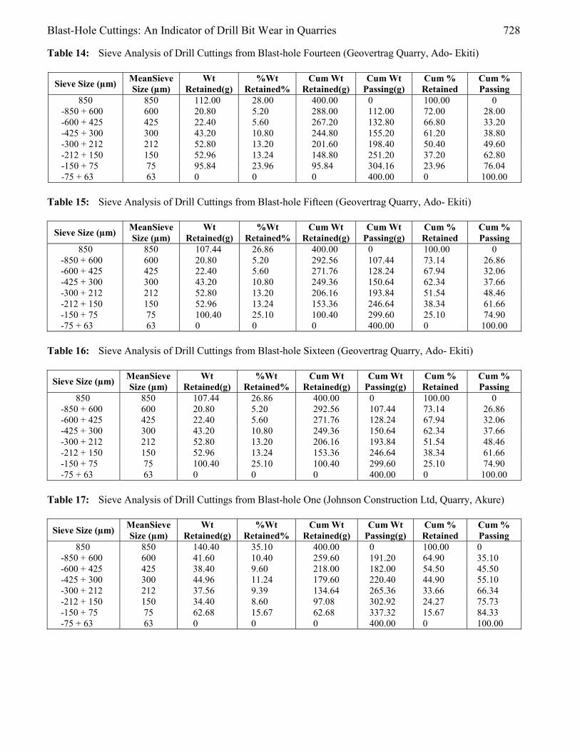
Table 14: Sieve Analysis of Drill Cuttings from Blast-hole Fourteen (Geovertrag Quarry, Ado- Ekiti)
Sieve Size (µm) MeanSieve Size (µm)
Wt Retained(g)
%Wt Retained%
Cum Wt Retained(g)
Cum Wt Passing(g)
Cum % Retained
Cum % Passing
850 850 112.00 28.00 400.00 0 100.00 0 -850 + 600 600 20.80 5.20 288.00 112.00 72.00 28.00 -600 + 425 425 22.40 5.60 267.20 132.80 66.80 33.20 -425 + 300 300 43.20 10.80 244.80 155.20 61.20 38.80 -300 + 212 212 52.80 13.20 201.60 198.40 50.40 49.60 -212 + 150 150 52.96 13.24 148.80 251.20 37.20 62.80 -150 + 75 75 95.84 23.96 95.84 304.16 23.96 76.04 -75 + 63 63 0 0 0 400.00 0 100.00
Table 15: Sieve Analysis of Drill Cuttings from Blast-hole Fifteen (Geovertrag Quarry, Ado- Ekiti)
Sieve Size (µm) MeanSieve Size (µm)
Wt Retained(g)
%Wt Retained%
Cum Wt Retained(g)
Cum Wt Passing(g)
Cum % Retained
Cum % Passing
850 850 107.44 26.86 400.00 0 100.00 0 -850 + 600 600 20.80 5.20 292.56 107.44 73.14 26.86 -600 + 425 425 22.40 5.60 271.76 128.24 67.94 32.06 -425 + 300 300 43.20 10.80 249.36 150.64 62.34 37.66 -300 + 212 212 52.80 13.20 206.16 193.84 51.54 48.46 -212 + 150 150 52.96 13.24 153.36 246.64 38.34 61.66 -150 + 75 75 100.40 25.10 100.40 299.60 25.10 74.90 -75 + 63 63 0 0 0 400.00 0 100.00
Table 16: Sieve Analysis of Drill Cuttings from Blast-hole Sixteen (Geovertrag Quarry, Ado- Ekiti)
Sieve Size (µm) MeanSieve Size (µm)
Wt Retained(g)
%Wt Retained%
Cum Wt Retained(g)
Cum Wt Passing(g)
Cum % Retained
Cum % Passing
850 850 107.44 26.86 400.00 0 100.00 0 -850 + 600 600 20.80 5.20 292.56 107.44 73.14 26.86 -600 + 425 425 22.40 5.60 271.76 128.24 67.94 32.06 -425 + 300 300 43.20 10.80 249.36 150.64 62.34 37.66 -300 + 212 212 52.80 13.20 206.16 193.84 51.54 48.46 -212 + 150 150 52.96 13.24 153.36 246.64 38.34 61.66 -150 + 75 75 100.40 25.10 100.40 299.60 25.10 74.90 -75 + 63 63 0 0 0 400.00 0 100.00
Table 17: Sieve Analysis of Drill Cuttings from Blast-hole One (Johnson Construction Ltd, Quarry, Akure)
Sieve Size (µm) MeanSieve Size (µm)
Wt Retained(g)
%Wt Retained%
Cum Wt Retained(g)
Cum Wt Passing(g)
Cum % Retained
Cum % Passing
850 850 140.40 35.10 400.00 0 100.00 0 -850 + 600 600 41.60 10.40 259.60 191.20 64.90 35.10 -600 + 425 425 38.40 9.60 218.00 182.00 54.50 45.50 -425 + 300 300 44.96 11.24 179.60 220.40 44.90 55.10 -300 + 212 212 37.56 9.39 134.64 265.36 33.66 66.34 -212 + 150 150 34.40 8.60 97.08 302.92 24.27 75.73 -150 + 75 75 62.68 15.67 62.68 337.32 15.67 84.33 -75 + 63 63 0 0 0 400.00 0 100.00

729 Z.O. Opafunso and B. Adebayo
Table 18: Sieve Analysis of Drill Cuttings from Blast-hole Two (Johnson Construction Ltd, Quarry, Akure)
Sieve Size (µm) MeanSieve Size (µm)
Wt Retained(g)
%Wt Retained%
Cum Wt Retained(g)
Cum Wt Passing(g)
Cum % Retained
Cum % Passing
850 850 136.68 34.17 400.00 0 100.00 0 -850 + 600 600 40.80 10.20 263.32 136.68 65.83 34.17 -600 + 425 425 34.24 8.56 222.52 177.48 55.63 44.37 -425 + 300 300 43.32 10.83 188.28 211.72 47.07 52.93 -300 + 212 212 41.00 10.25 144.28 255.04 36.24 63.76 -212 + 150 150 39.12 9.78 103.96 296.04 25.99 74.01 -150 + 75 75 64.84 16.21 64.84 335.16 16.21 83.79 -75 + 63 63 0 0 0 400.00 0 100.00
Table 19: Sieve Analysis of Drill Cuttings from Blast-hole Three (Johnson Construction Ltd, Quarry, Akure)
Sieve Size (µm) MeanSieve Size (µm)
Wt Retained(g)
%Wt Retained%
Cum Wt Retained(g)
Cum Wt Passing(g)
Cum % Retained
Cum % Passing
850 850 132.80 33.20 400.00 0 100.00 0 -850 + 600 600 38.40 9.60 267.20 132.8 66.80 33.20 -600 + 425 425 34.80 8.70 228.80 171.20 57.20 42.80 -425 + 300 300 39.36 9.84 194.00 206.00 48.50 51.50 -300 + 212 212 40.80 10.20 154.64 245.36 38.66 61.34 -212 + 150 150 36.40 9.10 113.84 286.16 28.46 71.54 -150 + 75 75 77.44 19.36 77.44 322.56 19.36 80.64 -75 + 63 63 0 0 0 400.00 0 100.00
Table 20: Sieve Analysis of Drill Cuttings from Blast-hole Four (Johnson Construction Ltd, Quarry, Akure)
Sieve Size (µm) MeanSieve Size (µm)
Wt Retained(g)
%Wt Retained
Cum Wt Retained(g)
Cum wt Passing(g)
Cum % Retained
Cum % Passing
850 850 128.00 32.00 400.00 0 100.00 0 -850 +600 600 35.60 8.90 272.00 128.00 68.00 32.00 -600+ 425 425 32.00 8.00 236.40 163.60 59.10 40.90 -425 +300 300 40.72 10.18 204.40 195.60 51.10 48.90 -300 +212 212 42.72 10.68 163.68 236.32 40.92 59.08 -212 +150 150 38.00 9.50 120.96 279.04 30.24 69.76 -150 + 75 75 82.96 20.74 82.96 317.04 20.74 79.26 -75 + 63 63 0 0 0 400.00 0 100.00
Table 21: Sieve Analysis of Drill Cuttings from Blast-hole Five (Johnson Construction Ltd, Quarry, Akure)
Sieve Size (µm) MeanSieve Size (µm)
Wt Retained(g)
%Wt Retained%
Cum Wt Retained(g)
Cum Wt Passing(g)
Cum % Retained
Cum % Passing
850 850 126.00 31.50 400.00 0 100.00 0 -850 + 600 600 34.00 8.50 274.00 126.00 68.50 31.50 -600 + 425 425 32.00 8.00 240.00 160.00 60.00 40.00 -425 + 300 300 40.32 10.08 208.00 192.00 52.00 48.00 -300 + 212 212 43.52 10.88 167.68 232.32 41.92 58.08 -212 + 150 150 39.20 9.80 124.16 275.84 31.04 68.96 -150 + 75 75 84.96 21.24 84.96 315.04 21.24 78.76 -75 + 63 63 0 0 0 400.00 0 100.00
Blast-Hole Cuttings: An Indicator of Drill Bit Wear in Quarries 730
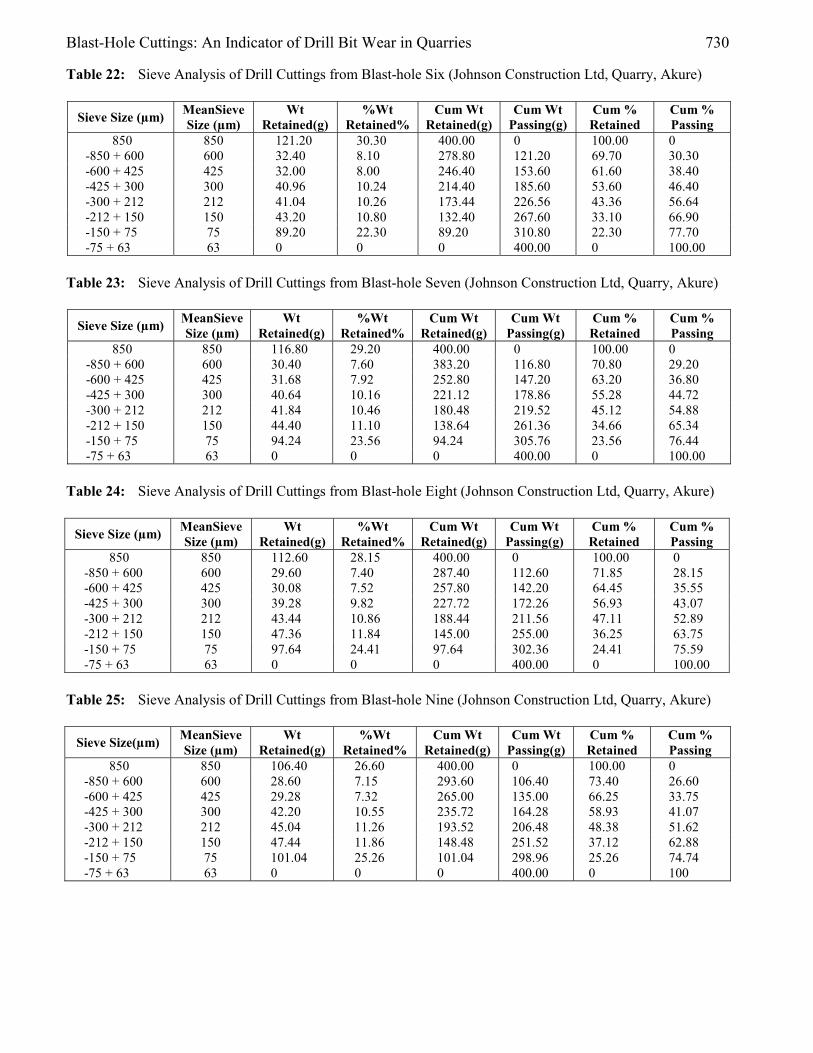
Table 22: Sieve Analysis of Drill Cuttings from Blast-hole Six (Johnson Construction Ltd, Quarry, Akure)
Sieve Size (µm) MeanSieve Size (µm)
Wt Retained(g)
%Wt Retained%
Cum Wt Retained(g)
Cum Wt Passing(g)
Cum % Retained
Cum % Passing
850 850 121.20 30.30 400.00 0 100.00 0 -850 + 600 600 32.40 8.10 278.80 121.20 69.70 30.30 -600 + 425 425 32.00 8.00 246.40 153.60 61.60 38.40 -425 + 300 300 40.96 10.24 214.40 185.60 53.60 46.40 -300 + 212 212 41.04 10.26 173.44 226.56 43.36 56.64 -212 + 150 150 43.20 10.80 132.40 267.60 33.10 66.90 -150 + 75 75 89.20 22.30 89.20 310.80 22.30 77.70 -75 + 63 63 0 0 0 400.00 0 100.00
Table 23: Sieve Analysis of Drill Cuttings from Blast-hole Seven (Johnson Construction Ltd, Quarry, Akure)
Sieve Size (µm) MeanSieve Size (µm)
Wt Retained(g)
%Wt Retained%
Cum Wt Retained(g)
Cum Wt Passing(g)
Cum % Retained
Cum % Passing
850 850 116.80 29.20 400.00 0 100.00 0 -850 + 600 600 30.40 7.60 383.20 116.80 70.80 29.20 -600 + 425 425 31.68 7.92 252.80 147.20 63.20 36.80 -425 + 300 300 40.64 10.16 221.12 178.86 55.28 44.72 -300 + 212 212 41.84 10.46 180.48 219.52 45.12 54.88 -212 + 150 150 44.40 11.10 138.64 261.36 34.66 65.34 -150 + 75 75 94.24 23.56 94.24 305.76 23.56 76.44 -75 + 63 63 0 0 0 400.00 0 100.00
Table 24: Sieve Analysis of Drill Cuttings from Blast-hole Eight (Johnson Construction Ltd, Quarry, Akure)
Sieve Size (µm) MeanSieve Size (µm)
Wt Retained(g)
%Wt Retained%
Cum Wt Retained(g)
Cum Wt Passing(g)
Cum % Retained
Cum % Passing
850 850 112.60 28.15 400.00 0 100.00 0 -850 + 600 600 29.60 7.40 287.40 112.60 71.85 28.15 -600 + 425 425 30.08 7.52 257.80 142.20 64.45 35.55 -425 + 300 300 39.28 9.82 227.72 172.26 56.93 43.07 -300 + 212 212 43.44 10.86 188.44 211.56 47.11 52.89 -212 + 150 150 47.36 11.84 145.00 255.00 36.25 63.75 -150 + 75 75 97.64 24.41 97.64 302.36 24.41 75.59 -75 + 63 63 0 0 0 400.00 0 100.00
Table 25: Sieve Analysis of Drill Cuttings from Blast-hole Nine (Johnson Construction Ltd, Quarry, Akure)
Sieve Size(µm) MeanSieve Size (µm)
Wt Retained(g)
%Wt Retained%
Cum Wt Retained(g)
Cum Wt Passing(g)
Cum % Retained
Cum % Passing
850 850 106.40 26.60 400.00 0 100.00 0 -850 + 600 600 28.60 7.15 293.60 106.40 73.40 26.60 -600 + 425 425 29.28 7.32 265.00 135.00 66.25 33.75 -425 + 300 300 42.20 10.55 235.72 164.28 58.93 41.07 -300 + 212 212 45.04 11.26 193.52 206.48 48.38 51.62 -212 + 150 150 47.44 11.86 148.48 251.52 37.12 62.88 -150 + 75 75 101.04 25.26 101.04 298.96 25.26 74.74 -75 + 63 63 0 0 0 400.00 0 100
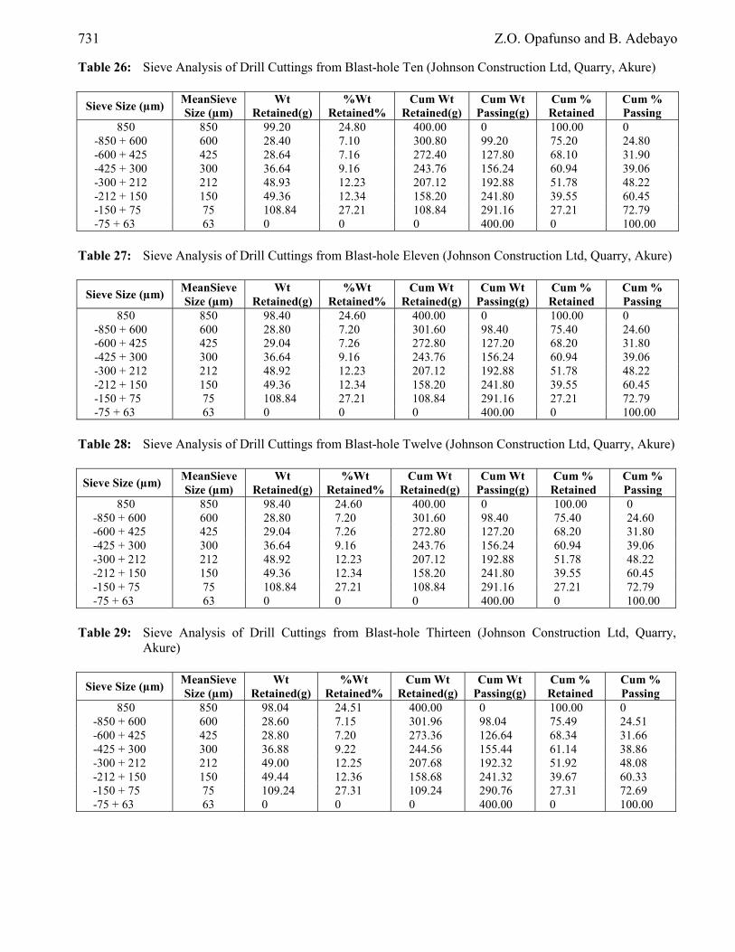
731 Z.O. Opafunso and B. Adebayo
Table 26: Sieve Analysis of Drill Cuttings from Blast-hole Ten (Johnson Construction Ltd, Quarry, Akure)
Sieve Size (µm) MeanSieve Size (µm)
Wt Retained(g)
%Wt Retained%
Cum Wt Retained(g)
Cum Wt Passing(g)
Cum % Retained
Cum % Passing
850 850 99.20 24.80 400.00 0 100.00 0 -850 + 600 600 28.40 7.10 300.80 99.20 75.20 24.80 -600 + 425 425 28.64 7.16 272.40 127.80 68.10 31.90 -425 + 300 300 36.64 9.16 243.76 156.24 60.94 39.06 -300 + 212 212 48.93 12.23 207.12 192.88 51.78 48.22 -212 + 150 150 49.36 12.34 158.20 241.80 39.55 60.45 -150 + 75 75 108.84 27.21 108.84 291.16 27.21 72.79 -75 + 63 63 0 0 0 400.00 0 100.00
Table 27: Sieve Analysis of Drill Cuttings from Blast-hole Eleven (Johnson Construction Ltd, Quarry, Akure)
Sieve Size (µm) MeanSieve Size (µm)
Wt Retained(g)
%Wt Retained%
Cum Wt Retained(g)
Cum Wt Passing(g)
Cum % Retained
Cum % Passing
850 850 98.40 24.60 400.00 0 100.00 0 -850 + 600 600 28.80 7.20 301.60 98.40 75.40 24.60 -600 + 425 425 29.04 7.26 272.80 127.20 68.20 31.80 -425 + 300 300 36.64 9.16 243.76 156.24 60.94 39.06 -300 + 212 212 48.92 12.23 207.12 192.88 51.78 48.22 -212 + 150 150 49.36 12.34 158.20 241.80 39.55 60.45 -150 + 75 75 108.84 27.21 108.84 291.16 27.21 72.79 -75 + 63 63 0 0 0 400.00 0 100.00
Table 28: Sieve Analysis of Drill Cuttings from Blast-hole Twelve (Johnson Construction Ltd, Quarry, Akure) Sieve Size (µm) MeanSieve
Size (µm) Wt
Retained(g) %Wt
Retained% Cum Wt
Retained(g) Cum Wt
Passing(g) Cum % Retained
Cum % Passing
850 850 98.40 24.60 400.00 0 100.00 0 -850 + 600 600 28.80 7.20 301.60 98.40 75.40 24.60 -600 + 425 425 29.04 7.26 272.80 127.20 68.20 31.80 -425 + 300 300 36.64 9.16 243.76 156.24 60.94 39.06 -300 + 212 212 48.92 12.23 207.12 192.88 51.78 48.22 -212 + 150 150 49.36 12.34 158.20 241.80 39.55 60.45 -150 + 75 75 108.84 27.21 108.84 291.16 27.21 72.79 -75 + 63 63 0 0 0 400.00 0 100.00
Table 29: Sieve Analysis of Drill Cuttings from Blast-hole Thirteen (Johnson Construction Ltd, Quarry,
Akure)
Sieve Size (µm) MeanSieve Size (µm)
Wt Retained(g)
%Wt Retained%
Cum Wt Retained(g)
Cum Wt Passing(g)
Cum % Retained
Cum % Passing
850 850 98.04 24.51 400.00 0 100.00 0 -850 + 600 600 28.60 7.15 301.96 98.04 75.49 24.51 -600 + 425 425 28.80 7.20 273.36 126.64 68.34 31.66 -425 + 300 300 36.88 9.22 244.56 155.44 61.14 38.86 -300 + 212 212 49.00 12.25 207.68 192.32 51.92 48.08 -212 + 150 150 49.44 12.36 158.68 241.32 39.67 60.33 -150 + 75 75 109.24 27.31 109.24 290.76 27.31 72.69 -75 + 63 63 0 0 0 400.00 0 100.00
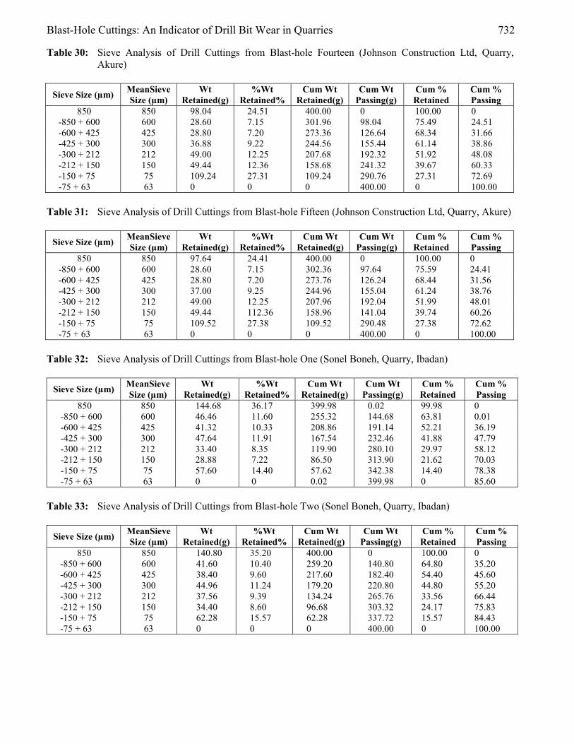
Blast-Hole Cuttings: An Indicator of Drill Bit Wear in Quarries 732
Table 30: Sieve Analysis of Drill Cuttings from Blast-hole Fourteen (Johnson Construction Ltd, Quarry, Akure)
Sieve Size (µm) MeanSieve
Size (µm) Wt
Retained(g) %Wt
Retained% Cum Wt
Retained(g) Cum Wt
Passing(g) Cum % Retained
Cum % Passing
850 850 98.04 24.51 400.00 0 100.00 0 -850 + 600 600 28.60 7.15 301.96 98.04 75.49 24.51 -600 + 425 425 28.80 7.20 273.36 126.64 68.34 31.66 -425 + 300 300 36.88 9.22 244.56 155.44 61.14 38.86 -300 + 212 212 49.00 12.25 207.68 192.32 51.92 48.08 -212 + 150 150 49.44 12.36 158.68 241.32 39.67 60.33 -150 + 75 75 109.24 27.31 109.24 290.76 27.31 72.69 -75 + 63 63 0 0 0 400.00 0 100.00
Table 31: Sieve Analysis of Drill Cuttings from Blast-hole Fifteen (Johnson Construction Ltd, Quarry, Akure)
Sieve Size (µm) MeanSieve Size (µm)
Wt Retained(g)
%Wt Retained%
Cum Wt Retained(g)
Cum Wt Passing(g)
Cum % Retained
Cum % Passing
850 850 97.64 24.41 400.00 0 100.00 0 -850 + 600 600 28.60 7.15 302.36 97.64 75.59 24.41 -600 + 425 425 28.80 7.20 273.76 126.24 68.44 31.56 -425 + 300 300 37.00 9.25 244.96 155.04 61.24 38.76 -300 + 212 212 49.00 12.25 207.96 192.04 51.99 48.01 -212 + 150 150 49.44 112.36 158.96 141.04 39.74 60.26 -150 + 75 75 109.52 27.38 109.52 290.48 27.38 72.62 -75 + 63 63 0 0 0 400.00 0 100.00
Table 32: Sieve Analysis of Drill Cuttings from Blast-hole One (Sonel Boneh, Quarry, Ibadan)
Sieve Size (µm) MeanSieve Size (µm)
Wt Retained(g)
%Wt Retained%
Cum Wt Retained(g)
Cum Wt Passing(g)
Cum % Retained
Cum % Passing
850 850 144.68 36.17 399.98 0.02 99.98 0 -850 + 600 600 46.46 11.60 255.32 144.68 63.81 0.01 -600 + 425 425 41.32 10.33 208.86 191.14 52.21 36.19 -425 + 300 300 47.64 11.91 167.54 232.46 41.88 47.79 -300 + 212 212 33.40 8.35 119.90 280.10 29.97 58.12 -212 + 150 150 28.88 7.22 86.50 313.90 21.62 70.03 -150 + 75 75 57.60 14.40 57.62 342.38 14.40 78.38 -75 + 63 63 0 0 0.02 399.98 0 85.60
Table 33: Sieve Analysis of Drill Cuttings from Blast-hole Two (Sonel Boneh, Quarry, Ibadan)
Sieve Size (µm) MeanSieve Size (µm)
Wt Retained(g)
%Wt Retained%
Cum Wt Retained(g)
Cum Wt Passing(g)
Cum % Retained
Cum % Passing
850 850 140.80 35.20 400.00 0 100.00 0 -850 + 600 600 41.60 10.40 259.20 140.80 64.80 35.20 -600 + 425 425 38.40 9.60 217.60 182.40 54.40 45.60 -425 + 300 300 44.96 11.24 179.20 220.80 44.80 55.20 -300 + 212 212 37.56 9.39 134.24 265.76 33.56 66.44 -212 + 150 150 34.40 8.60 96.68 303.32 24.17 75.83 -150 + 75 75 62.28 15.57 62.28 337.72 15.57 84.43 -75 + 63 63 0 0 0 400.00 0 100.00
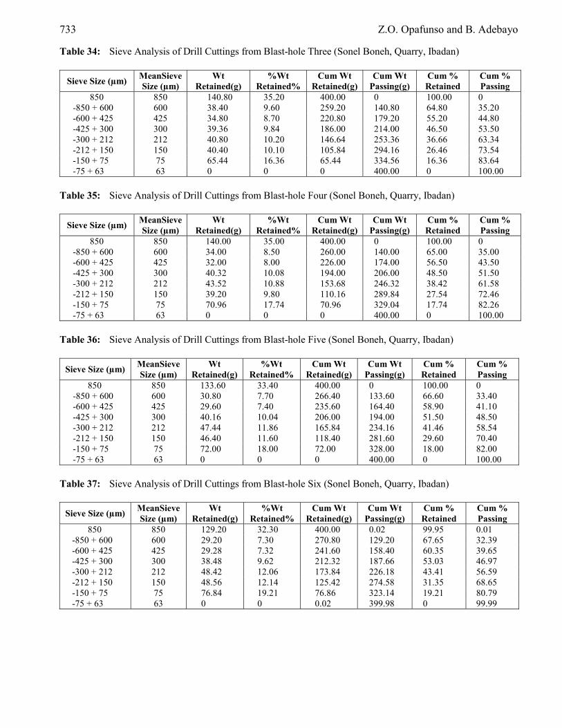
733 Z.O. Opafunso and B. Adebayo
Table 34: Sieve Analysis of Drill Cuttings from Blast-hole Three (Sonel Boneh, Quarry, Ibadan)
Sieve Size (µm) MeanSieve Size (µm)
Wt Retained(g)
%Wt Retained%
Cum Wt Retained(g)
Cum Wt Passing(g)
Cum % Retained
Cum % Passing
850 850 140.80 35.20 400.00 0 100.00 0 -850 + 600 600 38.40 9.60 259.20 140.80 64.80 35.20 -600 + 425 425 34.80 8.70 220.80 179.20 55.20 44.80 -425 + 300 300 39.36 9.84 186.00 214.00 46.50 53.50 -300 + 212 212 40.80 10.20 146.64 253.36 36.66 63.34 -212 + 150 150 40.40 10.10 105.84 294.16 26.46 73.54 -150 + 75 75 65.44 16.36 65.44 334.56 16.36 83.64 -75 + 63 63 0 0 0 400.00 0 100.00
Table 35: Sieve Analysis of Drill Cuttings from Blast-hole Four (Sonel Boneh, Quarry, Ibadan)
Sieve Size (µm) MeanSieve Size (µm)
Wt Retained(g)
%Wt Retained%
Cum Wt Retained(g)
Cum Wt Passing(g)
Cum % Retained
Cum % Passing
850 850 140.00 35.00 400.00 0 100.00 0 -850 + 600 600 34.00 8.50 260.00 140.00 65.00 35.00 -600 + 425 425 32.00 8.00 226.00 174.00 56.50 43.50 -425 + 300 300 40.32 10.08 194.00 206.00 48.50 51.50 -300 + 212 212 43.52 10.88 153.68 246.32 38.42 61.58 -212 + 150 150 39.20 9.80 110.16 289.84 27.54 72.46 -150 + 75 75 70.96 17.74 70.96 329.04 17.74 82.26 -75 + 63 63 0 0 0 400.00 0 100.00
Table 36: Sieve Analysis of Drill Cuttings from Blast-hole Five (Sonel Boneh, Quarry, Ibadan)
Sieve Size (µm) MeanSieve Size (µm)
Wt Retained(g)
%Wt Retained%
Cum Wt Retained(g)
Cum Wt Passing(g)
Cum % Retained
Cum % Passing
850 850 133.60 33.40 400.00 0 100.00 0 -850 + 600 600 30.80 7.70 266.40 133.60 66.60 33.40 -600 + 425 425 29.60 7.40 235.60 164.40 58.90 41.10 -425 + 300 300 40.16 10.04 206.00 194.00 51.50 48.50 -300 + 212 212 47.44 11.86 165.84 234.16 41.46 58.54 -212 + 150 150 46.40 11.60 118.40 281.60 29.60 70.40 -150 + 75 75 72.00 18.00 72.00 328.00 18.00 82.00 -75 + 63 63 0 0 0 400.00 0 100.00
Table 37: Sieve Analysis of Drill Cuttings from Blast-hole Six (Sonel Boneh, Quarry, Ibadan)
Sieve Size (µm) MeanSieve Size (µm)
Wt Retained(g)
%Wt Retained%
Cum Wt Retained(g)
Cum Wt Passing(g)
Cum % Retained
Cum % Passing
850 850 129.20 32.30 400.00 0.02 99.95 0.01 -850 + 600 600 29.20 7.30 270.80 129.20 67.65 32.39 -600 + 425 425 29.28 7.32 241.60 158.40 60.35 39.65 -425 + 300 300 38.48 9.62 212.32 187.66 53.03 46.97 -300 + 212 212 48.42 12.06 173.84 226.18 43.41 56.59 -212 + 150 150 48.56 12.14 125.42 274.58 31.35 68.65 -150 + 75 75 76.84 19.21 76.86 323.14 19.21 80.79 -75 + 63 63 0 0 0.02 399.98 0 99.99
Blast-Hole Cuttings: An Indicator of Drill Bit Wear in Quarries 734
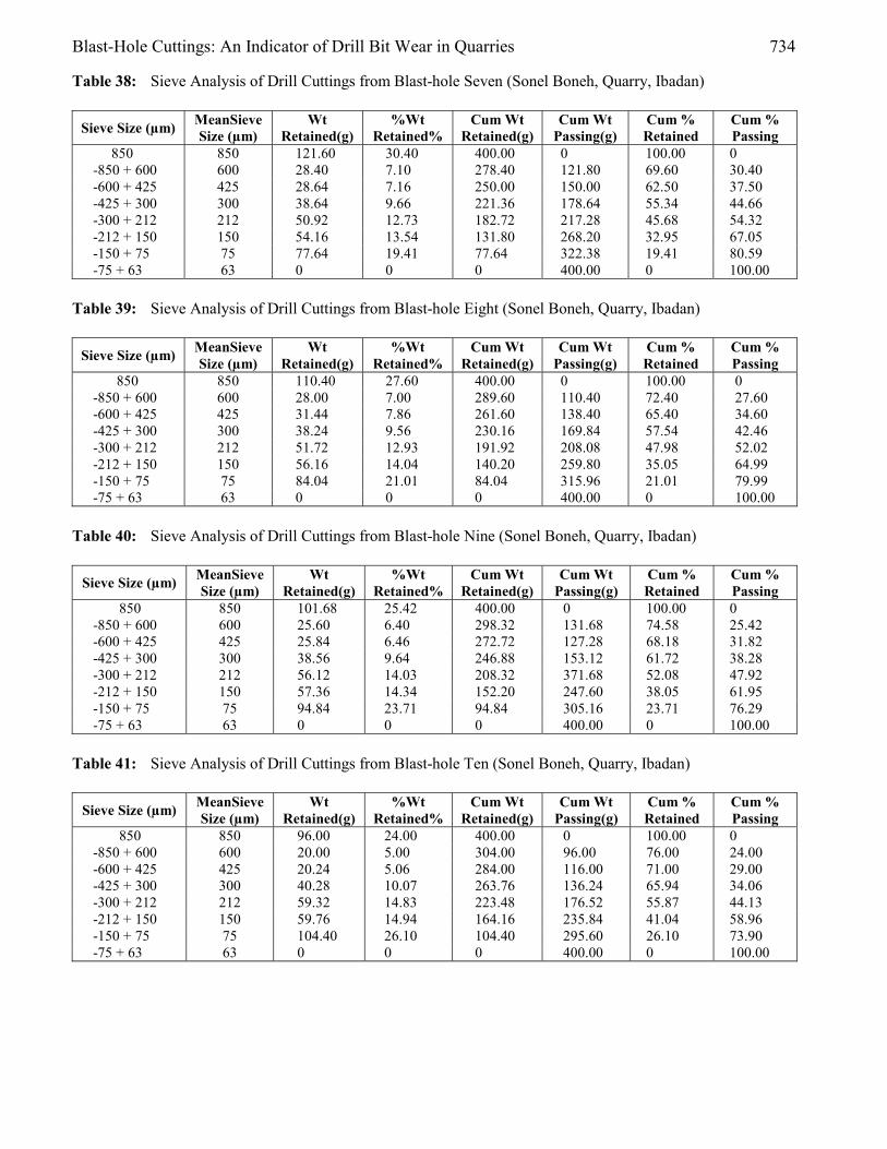
Table 38: Sieve Analysis of Drill Cuttings from Blast-hole Seven (Sonel Boneh, Quarry, Ibadan)
Sieve Size (µm) MeanSieve Size (µm)
Wt Retained(g)
%Wt Retained%
Cum Wt Retained(g)
Cum Wt Passing(g)
Cum % Retained
Cum % Passing
850 850 121.60 30.40 400.00 0 100.00 0 -850 + 600 600 28.40 7.10 278.40 121.80 69.60 30.40 -600 + 425 425 28.64 7.16 250.00 150.00 62.50 37.50 -425 + 300 300 38.64 9.66 221.36 178.64 55.34 44.66 -300 + 212 212 50.92 12.73 182.72 217.28 45.68 54.32 -212 + 150 150 54.16 13.54 131.80 268.20 32.95 67.05 -150 + 75 75 77.64 19.41 77.64 322.38 19.41 80.59 -75 + 63 63 0 0 0 400.00 0 100.00
Table 39: Sieve Analysis of Drill Cuttings from Blast-hole Eight (Sonel Boneh, Quarry, Ibadan)
Sieve Size (µm) MeanSieve Size (µm)
Wt Retained(g)
%Wt Retained%
Cum Wt Retained(g)
Cum Wt Passing(g)
Cum % Retained
Cum % Passing
850 850 110.40 27.60 400.00 0 100.00 0 -850 + 600 600 28.00 7.00 289.60 110.40 72.40 27.60 -600 + 425 425 31.44 7.86 261.60 138.40 65.40 34.60 -425 + 300 300 38.24 9.56 230.16 169.84 57.54 42.46 -300 + 212 212 51.72 12.93 191.92 208.08 47.98 52.02 -212 + 150 150 56.16 14.04 140.20 259.80 35.05 64.99 -150 + 75 75 84.04 21.01 84.04 315.96 21.01 79.99 -75 + 63 63 0 0 0 400.00 0 100.00
Table 40: Sieve Analysis of Drill Cuttings from Blast-hole Nine (Sonel Boneh, Quarry, Ibadan)
Sieve Size (µm) MeanSieve Size (µm)
Wt Retained(g)
%Wt Retained%
Cum Wt Retained(g)
Cum Wt Passing(g)
Cum % Retained
Cum % Passing
850 850 101.68 25.42 400.00 0 100.00 0 -850 + 600 600 25.60 6.40 298.32 131.68 74.58 25.42 -600 + 425 425 25.84 6.46 272.72 127.28 68.18 31.82 -425 + 300 300 38.56 9.64 246.88 153.12 61.72 38.28 -300 + 212 212 56.12 14.03 208.32 371.68 52.08 47.92 -212 + 150 150 57.36 14.34 152.20 247.60 38.05 61.95 -150 + 75 75 94.84 23.71 94.84 305.16 23.71 76.29 -75 + 63 63 0 0 0 400.00 0 100.00
Table 41: Sieve Analysis of Drill Cuttings from Blast-hole Ten (Sonel Boneh, Quarry, Ibadan)
Sieve Size (µm) MeanSieve Size (µm)
Wt Retained(g)
%Wt Retained%
Cum Wt Retained(g)
Cum Wt Passing(g)
Cum % Retained
Cum % Passing
850 850 96.00 24.00 400.00 0 100.00 0 -850 + 600 600 20.00 5.00 304.00 96.00 76.00 24.00 -600 + 425 425 20.24 5.06 284.00 116.00 71.00 29.00 -425 + 300 300 40.28 10.07 263.76 136.24 65.94 34.06 -300 + 212 212 59.32 14.83 223.48 176.52 55.87 44.13 -212 + 150 150 59.76 14.94 164.16 235.84 41.04 58.96 -150 + 75 75 104.40 26.10 104.40 295.60 26.10 73.90 -75 + 63 63 0 0 0 400.00 0 100.00

735 Z.O. Opafunso and B. Adebayo
Table 42: Sieve Analysis of Drill Cuttings from Blast-hole Eleven (Sonel Boneh, Quarry, Ibadan)
Sieve Size (µm) MeanSieve Size (µm)
Wt Retained(g)
%Wt Retained%
Cum Wt Retained(g)
Cum Wt Passing(g)
Cum % Retained
Cum % Passing
850 850 95.60 23.90 400.00 0 100.00 0 -850 + 600 600 19.60 4.90 304.40 95.60 76.10 23.90 -600 + 425 425 19.84 4.96 284.80 115.20 71.20 28.80 -425 + 300 300 40.28 10.07 264.96 135.04 66.24 33.76 -300 + 212 212 59.72 14.93 224.68 175.32 56.17 43.83 -212 + 150 150 60.16 15.04 164.96 235.04 41.24 58.76 -150 + 75 75 104.80 26.20 104.80 295.20 26.20 73.80 -75 + 63 63 0 0 0 400.00 0 100.00
Table 43: Sieve Analysis of Drill Cuttings from Blast-hole Twelve (Sonel Boneh, Quarry, Ibadan)
Sieve Size (µm) MeanSieve Size (µm)
Wt Retained(g)
%Wt Retained%
Cum Wt Retained(g)
Cum Wt Passing(g)
Cum % Retained
Cum % Passing
850 850 95.60 23.90 400.00 0 100.00 0 -850 + 600 600 19.60 4.90 304.40 95.60 76.10 23.90 -600 + 425 425 19.84 4.96 284.80 115.20 71.20 28.80 -425 + 300 300 40.28 10.07 264.96 135.04 66.24 33.76 -300 + 212 212 59.72 14.93 224.68 175.32 56.17 43.83 -212 + 150 150 60.16 15.04 164.96 235.04 41.24 58.76 -150 + 75 75 104.80 26.20 104.80 295.20 26.20 73.80 -75 + 63 63 0 0 0 400.00 0 100.00
Table 44: Sieve Analysis of Drill Cuttings from Blast-hole Thirteen (Sonel Boneh, Quarry, Ibadan)
Sieve Size (µm) MeanSieve Size (µm)
Wt Retained(g)
%Wt Retained%
Cum Wt Retained(g)
Cum Wt Passing(g)
Cum % Retained
Cum % Passing
850 850 95.20 23.80 400.00 0 100.00 0 -850 + 600 600 19.60 4.90 304.80 95.20 76.20 23.80 -600 + 425 425 19.44 4.86 285.20 114.80 71.30 28.70 -425 + 300 300 39.88 9.97 265.76 134.24 66.44 33.56 -300 + 212 212 60.12 15.03 225.88 174.12 56.47 43.53 -212 + 150 150 60.56 15.14 165.76 234.24 41.44 58.56 -150 + 75 75 105.20 26.30 105.20 294.80 26.30 73.70 -75 + 63 63 0 0 0 400.00 0 100.00
Table 45: Sieve Analysis of Drill Cuttings from Blast-hole Fourteen (Sonel Boneh, Quarry, Ibadan)
Sieve Size (µm) MeanSieve Size (µm)
Wt Retained(g)
%Wt Retained%
Cum Wt Retained(g)
Cum Wt Passing(g)
Cum % Retained
Cum % Passing
850 850 95.20 23.80 400.00 0 100.00 0 -850 + 600 600 19.60 4.90 304.80 95.20 76.20 23.80 -600 + 425 425 19.44 4.86 285.20 114.80 71.30 28.70 -425 + 300 300 39.88 9.97 265.76 134.24 66.44 33.56 -300 + 212 212 60.12 15.03 225.88 174.12 56.47 43.53 -212 + 150 150 60.56 15.14 165.76 234.24 41.44 58.56 -150 + 75 75 105.20 26.30 105.20 294.80 26.30 73.70 -75 + 63 63 0 0 0 400.00 0 100.00

Blast-Hole Cuttings: An Indicator of Drill Bit Wear in Quarries 736
Table 46: Sieve Analysis of Drill Cuttings from Blast-hole Fifteen (Sonel Boneh, Quarry, Ibadan)
Sieve Size (µm) MeanSieve Size (µm)
Wt Retained(g)
%Wt Retained%
Cum Wt Retained(g)
Cum Wt Passing(g)
Cum % Retained
Cum % Passing
850 850 94.80 23.70 400.00 0 100.00 0 -850 + 600 600 19.60 4.90 305.20 94.80 76.30 23.70 -600 + 425 425 19.44 4.86 228.50 114.40 71.40 28.60 -425 + 300 300 39.88 9.97 266.16 133.84 66.54 33.46 -300 + 212 212 60.52 15.13 226.28 173.72 56.57 43.43 -212 + 150 150 60.56 15.14 165.76 234.24 41.44 58.56 -150 + 75 75 105.20 26.30 105.20 294.80 26.30 73.70 -75 + 63 63 0 0 0 400.00 0 100.00
Conclusion The paper has examined the relationship between gauge button wear rate and blast-hole cuttings retained on 75µm sieve size. It was observed as bit buttons wear blast-hole cuttings become finer this is due to regrinding instead of penetrating the rock mass. Strong relationship exists between gauge bit button wear rate and weight of blast-hole cuttings retained on 75µm sieve size for the three selected quarries. References [1] Beste, U. (2004): On Nature of Cemented Carbide Wear in Rock Drilling, Doctorial Thesis,
Department of Engineering Science,Uppsala University Uppsala, Sweden. [2] Chiang, L.E. and Elias, D.A. (2000): Modelling Impact in Down-the-Hole Rock drilling,
International Journal of Rock Mechanics and Mining sciences, 37 (2000), pp 599-613. [3] Gokhale, B.V. (2004): Flushing of Blast-hole, http://rockproducts.com pp 1-4 [4] Hetenyi, M. (1966): Hand book of Experimental Stress Analysis, Wiley New-York, and 115
pp. [5] Howarth, D.F., Adamson, W.R. and Berndt, T.R. (1986): Correlation of Model Tunnel
Boring and Drilling Machine Performance with Rock Properties, International Journal of Rock Mechanics and Mining sciences, 23, pp 171-175 [Technical Note].
[6] Morley, A. (1944): Strength of Materials, Longman London, 35pp. [7] Shah, K.R. and Wong, T.F. (1997): Fracturing at Contact Surfaces Subjected to Normal and
Tangential Load, International Journal of Rock Mechanics, Mining sciences and Geomechanics, 1997; 3(5), pp 727-739.
[8] Thuro, K. (1997): Drillability Prediction - Geological Influences in Hard Rock Drill and Blast Tunneling, Geol. Rundsch 86, pp. 426 – 437.

European Journal of Scientific Research ISSN 1450-216X Vol.20 No.4 (2008), pp.737-745 © EuroJournals Publishing, Inc. 2008 http://www.eurojournals.com/ejsr.htm
Assessment of Micro-Credit Supply by Country Women
Association of Nigeria (Cowan) to Rural Women in Ondo State, Nigeria
M.G. Olujide Department of Agricultural Extension & Rural Development
University of Ibadan, Ibadan, Nigeria E-mail: [email protected], [email protected]
Abstract
Most Nigerian rural farmers are small scale farmers who require small amount of loan to help them improve their production. One of the avenue by which the rural women obtain loan is through the Country Women Association of Nigeria (COWAN).
This paper assessed the micro credit supply by COWAN to rural women in Ondo State, Nigeria and specifically find out demographic characteristics of respondents, examine the conditions for granting loan, attitude of the rural women towards COWAN micro credit scheme, ascertain amount of micro-credit provided, ways by which rural women utilizes the micro-credit, the timeliness of micro-credits and examine the constraints facing rural women towards getting the micro credit.
One hundred and six rural women was selected in four Local Government areas of Ondo state, using multi-stage random sampling technique.
The result revealed that majority (64.1%) of the rural women had age ranges between 21 and 40 years, 76.4% of them are married, 9.4% were single, 10.4% were divorced and the remaining 3.8% of them were divorced. Majority (78.3%) were Christians, had adult literacy 5.7%, 27.4% had primary education, 17% had secondary education, 16% of them had no formal education and 8.5% of them had higher education.
On the attitude of rural women, 16% of the respondents fall into the Low attitude score towards COWAN micro credit. The majority (84%) of them fall into high attitude score.
The result further revealed that 42.5% of the respondents obtained the sum of N5,000:00 – N10,000:00 as micro credit and 43.4% of them obtained the sum of N11,000:00 – N16,000:00 micro credit while 14.1% obtained above N16,000:00 as micro credit from COWAN.
The respondents used the micro credit obtained from COWAN for farming (85.5%) and remaining 14.5% of them for trading.
The constraints identified by respondents include lack of funds (37.7%), short period of repayment (28.7%) and Loan defaulters 16% as their major constraints. The benefits derived from COWAN micro credit include increase in production (75.5%).
The study revealed that marital status, age, position among husbands wife, number of children, educational level and religion have no significant relationship with the micro credit received from COWAN group while the occupation of the respondents has a significant relationship with the micro credit received.

Assessment of Micro-Credit Supply by Country Women Association of Nigeria (Cowan) to Rural Women in Ondo State, Nigeria 738
Based on the findings of the study, it is recommended that lump sum of money should be granted to rural women to enhance their productivity so as to change their living status. Keywords: Micro-Credit, Supply, COWAN and Rural Women.
Introduction Credit is the process of obtaining control over the use of money, good and services in the present in exchange for a promise to pay at a future date (Adegeye and Dittoh, 1985). It is a capital resources used in production that is a monetary resources, which can take the form of money in cash or bank draft or in kind as a firm of biological and physical purchased and supplied to producers.
The purpose of any saving and credit programme is to enable people gain access on reasonable terms to assets, which they can use to improve their livelihood. Virtually all societies, households and individual save and borrow money, saving take place during periods when income exceeds expenditure.
The micro credit scheme was an evolutionary process of merging and refining traditional and other practices which are indigenous to our people, an adapted to their most felt needs and experience. These traditional credit systems usually involve: a group of people pooling resources together; voluntary membership and consensus based on decision making; regular monetary contribution; and access to credit from group on rotational and interest-free basis.
Micro-credit programmes however extend small loan to people for employment project that generate income, allowing them to care for themselves and their family. In Nigeria, micro-credit programmes offer a combination of services and resources to their client in addition to credit. These often include saving facilities, training, networking and peer support (McKean, C.S. 1989).
According to Williams (1993) rural women are major contributors to subsistence agriculture as producers and marketers, they also engaged in keeping poultry, small animals such as sheep, goats, rabbits and dairy cattle. However, inspite of their prominent feature in agricultural production, they are usually under remunerated in terms of financial gains, social acceptability, appreciation and time taken off when compared with men (Aweto, 1996).
The basic assumption is that rural women are usually resource poor, lack necessary information to take vital decisions to improve their conditions of living and consequently do not have access to the government organs or agencies set up to ameliorate their hardship since rural women are known to be hard working, it is assumed that if their attitude are changed through training and they become exposed to the wherewithal by which they can improve their conditions, they will be motivated to engage more in enterprise development and consequently increase their income to enhance their standard of living (Brown, 1979). Hence, they will be able to decide on who to approach, for what, when and what to engage in. Therefore, COWAN intends to provide this vital linkage with resource input and equip rural women with the management skill required for successfully managing their income generating activities (Ogunleye, 2000).
The issue of micro-credit has been taking a centre stage of discussions on rural development and poverty alleviation, Non-governmental organization, governments, the people have discovered that for effective rural development to thrive, issues of micro credit should form a cardinal programme. Emerging trends have pointed to the fact that the role of micro-credit has became far from what is used to be considered as poverty alleviation strategies and as a vehicle for providing financial services to the poor (Olujide, 1999).
Micro-credit as it is often referred to has been adjudged as a catalyst for sustainable development. It goes beyond just a programme of economic empowerment that target saver and provision of credit transaction for low income and underprivileged groups to actual capacity building

739 M.G. Olujide
through the provision of technical assistance to the most vulnerable group with the classification of the poor (Imam, 1998).
The roles of micro-credit as a poverty alleviation strategy and a vehicle for providing financial services to the poor have continued to gain prominence in the society. The connect is not far fetched, this is because developing a broad based of micro-entrepreneurs in any economy is consequential to the sustenance of its growth and development process (Olujide, 1999).
The Country Women Association of Nigeria (COWAN) is an apex non-governmental organization for recognition and advancement of rural women in agriculture, economic and decision making for a total utilization and development of the nations vital human and natural resources and talent for self-reliance. It is COWANs vision to have a society free from indignity and oppression of peoples knowledge, elimination of hunger and poverty, economic injustice and inferiority complex, upholding peoples dignity, sense of belonging and ownership, designing with people a development process which embraces building self-sufficiency and sustainable development.
COWAN established in Ondo State in 1982, has consistently work hard to develop powerful tools to increase economic independence of rural women in Nigeria. These tools include a micro credit system which values, updates and combines indigenous micro-credit practices with aspects of modern banking system in a way that makes the resulting system deliver credit and related services to rural villages in a user-friendly way (COWAN, 2000). A unique characteristic of the micro-credit programme in the ownership of the financial institution by borrowers themselves.
COWAN has additionally organized rural women, updated their production skills, regularly advised them of economic opportunities and mobilize funds to expose its members to various national, regional and international workshops and conferences in an effort to update their knowledge and increase their networks (Ogunleye, 2000). COWAN, a non-governmental organization was set up with the primary concern of alleviating poverty among the rural women and to increase the economic independence of rural women in Nigeria (Ogunleye, 1997, Olujide 1999).
The micro credit supplied by COWAN has greatly increase the economic competence of rural women and has mobilized the traditional strength of Nigerian rural women to promote their participation in the development of human and natural sources for sustainable livelihood in rural and urban advocate for women economic and social empowerment.
Women feature in small-scale enterprises and this account for the smallness of their loans. The provision of credit to people with low income and poor educational background is generally not acceptable to formal institutions because of higher administrative costs and getting access to finance has not been easy for rural women.
Research had shown that women have very limited access to land, capital, gainful employment and positions of decision making (Christine, 1993 and Olawoye,2002). These constraints have drawn women to the informal sector to source for capital. This informal sector includes family, friends, private money-lenders, Esusu, cooperative societies. Apart from these sources, Non-governmental organizations and donor agencies have given out millions as grants to micro finance organizations to be given out as revolving loans to their members.
It is against the background that the following questions are posed in the study. 1. What are the demographic characteristics (age, marital status, religion, educational level,
occupation) of rural women? 2. What are the conditions for granting micro-credit to rural women? 3. What is the attitude of rural women towards the micro-credit programme? 4. What is the amount granted to micro-credit to rural women? 5. What purposes are the micro-credit utilized? 6. Is the provision of Micro-Credit to rural women by COWAN timely? 7. What are the constraints facing the rural women under the micro-credit programme?

Assessment of Micro-Credit Supply by Country Women Association of Nigeria (Cowan) to Rural Women in Ondo State, Nigeria 740 Objective of the Study The general objective of the study was to assess the micro-credit supply of COWAN to the rural women in Ondo State, Nigeria.
The specific objective include: 1. identify the demographic characteristics (such as age, marital status, religion, educational
level, occupation) of rural women. 2. examine the conditions for granting micro credit to rural women by COWAN. 3. examine the attitude of rural women towards micro credit programme. 4. ascertain if the amount of micro credit provided by COWAN is enough for rural women. 5. identify the ways by which rural women utilizes the Micro-credit. 6. ascertain the timeliness of micro-credit of COWAN, 7. examine the constraints faced by rural women towards getting the micro credit.
Methodology Area of the Study
The study was carried out in Ondo State of Nigeria. The State has eighteen (18) local government areas and is located in the South Western area of Nigeria and lies between latitude 7º’N and 4º 47’E longitude. The state experience two major seasons, dry and wet seasons which favour the growth of varieties of food and cash crops. The major economics activities of the people was farming and the major crops grown are yam, cassava, maize and vegetables while the cash crops include cocoa, oil palm, rubber and kolanut. Population and Sampling Procedure The population for this study are rural women in Ondo State who are members of COWAN group. Multi-stage sampling was employed for the study. The state was divided into four geographical zones with the eighteen local government areas. The first stage of the sampling involves selection of six Local Governmnt Areas from each zone Each of the geographical zone has an average of six local government areas which was randomly selected. In each local government area selected, there are four groups of COWAN with hundreds (100) members. Forty members were selected for the study representing 10% the population, making one hundred and six respondents as shown in table 1. Table 1: Analysis of Sample Selection
Selected Local Government Area Number of Programmes
Number of Programme
Selected
Number of Respondents in
Local Government
Sampled Respondents
1. Ondo West Local Government 4 1 150 30 2. Ilaje Local Government 3 1 100 25 3. Akure North Local Government 4 1 160 30 4. Akoko Southeast Local Government 4 1 150 21 Total 15 4 560 106
*Membership strength as contained in COWAN register. Source: Field Survey, 2006.
Data Collection Both primary and secondary data were used during the study. Respondents were interviewed using their responses as primary data, secondary data was obtained from records provided by COWAN, published articles and relevant texts.
741 M.G. Olujide
Analytical Techniques
The data obtained from interview schedule was subject to descriptive and inferential statistical analysis. Descriptive statistics for this study include frequency, percentages and means and the hypothesis was tested using chi-square. Result and Discussions
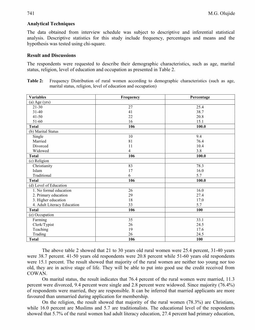
The respondents were requested to describe their demographic characteristics, such as age, marital status, religion, level of education and occupation as presented in Table 2. Table 2: Frequency Distribution of rural women according to demographic characteristics (such as age,
marital status, religion, level of education and occupation) Variables Frequency Percentage (a) Age (yrs)
21-30 27 25.4 31-40 41 38.7 41-50 22 20.8 51-60 16 15.1
Total 106 100.0 (b) Marital Status
Single 10 9.4 Married 81 76.4 Divorced 11 10.4 Widowed 4 3.8
Total 106 100.0 (c) Religion
Christianity 83 78.3 Islam 17 16.0 Traditional 6 5.7
Total 106 100.0 (d) Level of Education
1. No formal education 26 16.0 2. Primary education 29 27.4 3. Higher education 18 17.0 4. Adult Literacy Education 33 5.7
Total 106 100 (e) Occupation
Farming 35 33.1 Clerk/Typist 26 24.5 Teaching 19 17.6 Trading 26 24.5
Total 106 100
The above table 2 showed that 21 to 30 years old rural women were 25.4 percent, 31-40 years were 38.7 percent. 41-50 years old respondents were 20.8 percent while 51-60 years old respondents were 15.1 percent. The result showed that majority of the rural women are neither too young nor too old, they are in active stage of life. They will be able to put into good use the credit received from COWAN.
On marital status, the result indicates that 76.4 percent of the rural women were married, 11.3 percent were divorced, 9.4 percent were single and 2.8 percent were widowed. Since majority (76.4%) of respondents were married, they are responsible. It can be inferred that married applicants are more favoured than unmarried during application for membership.
On the religion, the result showed that majority of the rural women (78.3%) are Christians, while 16.0 percent are Muslims and 5.7 are traditionalists. The educational level of the respondents showed that 5.7% of the rural women had adult literacy education, 27.4 percent had primary education,

Assessment of Micro-Credit Supply by Country Women Association of Nigeria (Cowan) to Rural Women in Ondo State, Nigeria 742 17.0 percent had secondary education, 16.0 percent of them had no formal education and 8.5 percent respondents had higher education.
On the occupation of the rural women, the result showed that 33.0 percent of the rural women major occupation was farming, 24.5 percent of them are clerk/typists, 17.9 percent of the respondents are teachers and 24.5 percent respondents are traders. This indicates that COWAN takes care of various activities of women. Conditions for Giving Loan to Rural Women by Cowan
The conditions for giving loan to rural women by COWAN include the following: 1. You must be a registered COWAN member 2. Intending borrowers must be registered with COWAN organization in their community for
a period of 6 months and must apply for credit through their group. 3. Members must attend meeting regularly and pay monthly due of N100.00. 4. The duration for repaying monetary credit is one year and the interest rate was 10%. The attitude of rural women towards micro credit received from COWAN micro-credit was
categorized as unfavourable and favourable using attitudinal scores as shown in Table 3. Table 3: Frequency Distribution of rural women according to attitude towards COWAN Micro Credit
Attitude of Respondents toward COWAN micro-credit Frequency Percentages Unfavourable 17 16.0 Favourable 89 84.0 Total 106 100.0
Table 3 showed that 16.0 percent of the respondents fall into the low attitude score towards
COWAN micro credit. Also, the majority (84.0%) falls into high attitude score. This therefore, implies that the rural women had favourable attitude towards the micro credits received from COWAN.
The amount of Micro Credit received as credit from COWAN was presented in Table 4. Table 4: Frequency Distribution of rural women according to the amount received as credit from COWAN
Amount (N) Frequency Percentage 5,000 – 10,000 45 42.5 11,000 – 16,000 46 43.4 Above 16,000 15 14.1
Total 106 100.0
Table 4 showed that 42.5 percent of the respondents obtained the sum of N5,000 – N10,000 as micro-credit and 43.4 percent of the respondents obtained the sum of N11,000 – N16,000 micro-credit while 14.1 percent obtained above N16,000 as micro-credit from COWAN. Utilization of Micro Credit Received from COWAN The micro credit given to rural women can be put into various use depending on the occupation of the beneficiaries as shown in table 5:

743 M.G. Olujide
Table 5: Frequency distribution of respondents according to utilization of micro credit received from COWAN.
Occupation Frequency Percentage Farming 91 85.5 Trading 15 14.5 Local Crafts - - Total 106 100.0
The result showed that majority (85.5 percent) of the respondents used the micro credit
obtained from COWAN organization for farming, 14.5 percent of them used for trading. The implication of this is that majority of the respondents utilizes the micro credit obtained for their occupation.
Constraints Faced by Rural Women in Obtaining Micro Credit from constraints faced by rural women in obtaining micro-credit as shown in Table 6. Table 6: Frequency Distribution of Respondents According to Constraints Faced by Rural Women
Identified Constraints Frequency Percentages Lack of funds 40 37.7 Mismanagement of funds 10 9.5 Short period of repayment 30 28.3 Loan defaulters 17 16.0 Lack of incentive from the government 9 8.5 Total 106 100.0
Table 6 indicates that 37.7 percent of the respondents agreed that lack of funds from COWAN
is their major constraints while 28.3 percent agreed that short period of repayment of micro credits granted was their constraints and 16.0 percents opined that loan defaulters are the major constraints, and 9.5 percents claimed that mismanagement of funds is the major constraints they faced from COWAN and 8.5 percent opined that lack of incentives from government is their major constraints. Benefit Derived from Micro Credit Obtained by Rural Women from COWAN Benefit derived from micro-credit obtained by rural women were presented in Table 6. Table 7: Frequency Distribution of Respondents According to the Benefits erived from COWAN Credit
Benefits Derived Frequency Percentages Increase in Production 70 75.5 Procure more farm inputs 10 9.4 Input 16 15.1 No response 8 7.5 Total 106 100.0
Table 7 indicates that majority of the respondents 75.5 percent obtained the micro-credit to
increase their production while 9.4 percent respondents received it to procure more farm inputs, while 15.1 percent respondents obtained it during the money seasons.
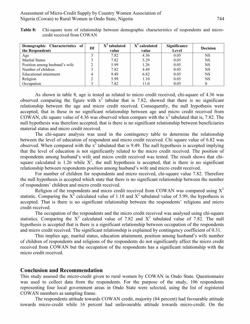
Assessment of Micro-Credit Supply by Country Women Association of Nigeria (Cowan) to Rural Women in Ondo State, Nigeria 744 Table 8: Chi-square tests of relationship between demographic characteristics of respondents and micro-
credit received from COWAN Demographic Characteristics of the Respondents Df X2 tabulated
value X2 calculated
value Significance
Level Decision
Age 3 7.82 4.36 0.05 NS Marital Status 3 7.82 5.29 0.05 NS Position among husband’s wife 2 5.99 1.26 0.05 NS Number of children 3 7.82 4.49 0.05 NS Educational attainment 4 9.49 6.82 0.05 NS Religion 2 5.99 1.10 0.05 NS Occupation 3 7.82 11.0 0.05 S
As shown in table 8, age is tested as related to micro credit received, chi-square of 4.36 was
observed comparing the figure with x2 tabular that is 7.82, showed that there is no significant relationship between the age and micro credit received. Consequently, the null hypothesis were accepted, that in these in no significant relationship between age and micro credit received from COWAN, chi square value of 4.36 was observed when compare with the x2 tabulated that is, 7.82. The null hypothesis was therefore accepted, that is there is no significant relationship between beneficiaries material status and micro credit received.
The chi-square analysis was used in the contingency table to determine the relationship between the level of education of respondent and micro credit received. Chi square value of 6.82 was observed. When compared with the x2 tabulated that is 9.49. The null hypothesis is accepted implying that the level of education is not significantly related to the micro credit received. The position of respondents among husband’s wife and micro credit received was tested. The result shows that chi-square calculated is 1.26 while X2, the null hypothesis is accepted, that is there is no significant relationship between respondents position among husband’s wife and micro credit received.
For number of children for respondents and micro received, chi-square value 7.82. Therefore the null hypothesis is accepted which state that there is no significant relationship between the number of respondents’ children and micro credit received.
Religion of the respondents and micro credit received from COWAN was compared using X2 statistic. Comparing the X2 calculated value of 1.10 and X2 tabulated value of 5.99, the hypothesis is accepted. That is there is no significant relationship between the respondents’ religions and micro credit received.
The occupation of the respondents and the micro credit received was analysed using chi-square statistics. Comparing the X2 calculated value of 7.82 and X2 tabulated value of 7.82. The null hypothesis is accepted that is there is a significant relationship between occupation of the respondents and micro credit received. The significant relationship is explained by contingency coefficient of 0.31.
This implies age, marital status, education attainment, position among husband’s wife number of children of respondents and religions of the respondents do not significantly affect the micro credit received from COWAN but the occupation of the respondents has a significant relationship with the micro credit received. Conclusion and Recommendation This study assesed the micro-credit given to rural women by COWAN in Ondo State. Questionnaire was used to collect data from the respondents. For the purpose of the study, 106 respondents representing four local government areas in Ondo State were selected, using the list of registered COWAN members as sampling frame.
The respondents attitude towards COWAN credit, majority (84 percent) had favourable attitude towards micro-credit while 16 percent had unfavourable attitude towards micro-credit. On the

745 M.G. Olujide
respondents benefit derived from the micro credit, majority (75.5 percent) of the respondents obtained the micro-credit to increase their production while 9 percent received it to procure more farm inputs and 15 percent did not respond to the variable.
On the constraints encountered by COWAN members 37.7 percent had inadequate funding as constraint, while 28.3 percent had constraint of short period of repayment of loan, 16 percent is attributed to loan defaulters, 9.5 percent is attributed to mismanagement of funds and 8.5 percent is attributed to lack of incentives from the government.
Based on the findings in this study, one can realize the COWAN is still bringing improvement to the living conditions of rural women. The rural women had benefited from the micro-credits granted to them by COWAN. It can be inferred that COWAN micro-credits had made impact among the rural women in the studied area. References [1] Adegeye and Ditto (1985). “Essential of Agricultural Economics”, Ibadan. Inpac Publisher
Limited, pp. 10-12. [2] Aweto, R.A. (1996). Agricultural Cooperatives. Stand and Printers. Builds Limited Ibadan. Pp.
141 – 142. [3] Brown, C.K. (1979). The participation of Women in Rural Development Programmes in
Kaduna State of Nigeria. C.S.E.R Research Pages 5, ABU, Zaria. Pp. 13. [4] Christine, Y. (1993). Investment Finance Off Limits for Women in Women and Economics
Policy. 0x 7am U.K. Edited by Barbara, pp. 16. [5] Imam. H. (1998): The role of Micro Credit in Development. Guardian Newspaper Vol. 4, No.
1237 pp. 10. [6] McKean, C.S. (1989). Training and Technical Assistance for Small and Micro business. A
review of their effectiveness and Implications for Women. Pp. 10 – 15. [7] Ogunleye, B. (2000). Innovation for Poverty Eradication. Country Women Association of
Nigeria. Presented at Micro-Credit Seminar. Washington DC, pp. 6-8. [8] Olawoye J.E(2002) Gender informed approaches to sustainable human development.Paper
presented at Workshop on gender issues in economic development,Organised by Nigerian centre for Economic Management and Administration(NCEMA)held at Ibadan.pp1-4
[9] Olujide, M.G. (1999). “Activities of Selected Non-Governmental Organisations (NGOs) in Rural Development in South West Nigeria (Ph.D. Thesis), Department of Agricultural Extension and Rural Development, University of Ibadan, Ibadan, pp. 104-110.
[10] Williams, C.E. (1982). The Status and Tasks of Rural Women In Nigeria: A Case Study of Allagba Village, Oyo State. Pp. 1 – 2.
European Journal of Scientific Research ISSN 1450-216X Vol.20 No.4 (2008), pp.746-758 © EuroJournals Publishing, Inc. 2008 http://www.eurojournals.com/ejsr.htm
Comparative Analysis of Pictorial Coverage of Events by
Pakistan’s English Press
Muhammad Nawaz Mahsud Chairman, Department of Communication Studies
University of Sargodha, Pakistan
Muhammad Khalid Professor, Department of Communication Studies
University of Sargodha, Pakistan
Firasat Jabeen Lecturer, Department of Communication Studies
University of Sargodha, Pakistan
Abstract
This study describes the leading English dailies ‘Dawn’ and ‘The Nation’ all pages pictorial coverage of events of international, national, provincial, and regional importance. Sixty newspapers containing 30 issues of each of the selected papers are analyzed. Results of the study show that daily ‘Dawn’ has significantly published more pictures and also spared significant space to developmental affairs, education, festival, disaster, accident, and crimes events compared to the number of pictures and space given to the same issues by daily “The Nation’ for the same period. Conversely daily ‘The Nation’ has published significantly more pictures and also given more space to the issues of politics, economics, technology, showbiz, health, war against terrorism, and sports than the number of pictures and space devoted to the same set of events by daily ‘Dawn.’ The results show no significant difference between both the papers’ coverage given to the events of environment, nature, weather, and others. The comparison of overall number of published pictures on events and space given to those pictures by the selected dailies shows significant difference. The Nation has published more number of pictures (930) and also spared significant space (223434) in centimeter compared to the Dawn number of pictures (712) and the space given to them (112669). It is also observed that both the papers have published significantly more pictures and also spared more space to the events of international importance than their number of pictures and space given to events of national, provincial, and regional importance.
Significance “One picture tells as much as 1000 words” (www.shipshapewsiebiz.com/NewsRoom.asp-20k). Human mind understands the language of pictures. Whatever we think, our mind creates pictures, and words transcend them into reality, making our ideas understandable. Most of the knowledge we perceive is through our sense of sight. “It is sense of sight that is dominant in human knowledge of the world, nature and life. Man actually receives two third of his knowledge through vision for what he sees is memorized easier. This is exactly why photography plays an important role in acquainting us with

Comparative Analysis of Pictorial Coverage of Events by Pakistan’s English Press 747
reality” (Hasan, 2005). Visuals are more effective, influential and memorable compared to the narration that is why most newspaper editors intend to accompany most of the news stories with pictures and special attention is given to the pictorial coverage of events so that the real picture of the event can be presented before the reader. There’s nothing like a photograph to give a newspaper motion and emotion. Photo journalism lies at the very heart of newspaper design” (Harrower, 2004). Today’s reader urges to see something unique, appealing, snappy, easy to grasp and that can appeal the reader’s aesthetic sense. ‘Every picture tells a story and every story deserves a picture. Today’s readers are so spoiled by TV and magazines that they now expect color photos, yet to accompany nearly every story they read’ (p.4).
Today’s media is entangled in competitive environment. Print media, newspaper in particular has to combat television staged with glamour, radio for its access, interactive media for its speed and glazing magazines. ‘Pictures are one of the key elements of a page. It is a picture that draws a reader into a page and helps to guide him or her through the page and the material on it’ (Frost, 2002). Therefore a right picture, at right place in right time plays pivotal role in making newspaper eye catching and can compete its other technological rivals. ‘It is one of the peculiar characteristics of the photo that it isolates single moments in time. The TV camera does not’ (McLuhan, 2002). It wouldn’t be wrong to say that pictures displayed in newspaper significantly attract more readerships. ‘The convincing power of the verbal comment in turn is strengthened by the photographic image, which multiplies the emotional elements’ (Hasan, 2005). This study aims to explore the coverage and importance given to the pictorial coverage by English dailies.
History of pictorial journalism is not so old. A French inventor named Niepce produced the first permanent photograph in 1826. The historian of photography associated with the rediscovery of Niepce’s early work was Helmut Gernsheim, whose History of Photography (published in 1995 and 1969) helped shape, for better or worse, the way that developments in the science are understood (Price 1998). Technological advancement in photographic equipments opened new doors of innovation, and it became possible to capture an event within a camera. The first newspaper photograph was published in 1880. News photos didn’t become common, however, until the early 1900s. Gradually photographs began to become important elements of newspaper design. Full color photos became common in the early’80s, thus ushering the modern era of newspaper design (Harrower, 2002). In Pakistan, during 1950s English newspapers followed this trend by giving occasional photographic coverage to important events. It took some time for Urdu newspaper to give attention to photography. However, in 1953, an Urdu daily ‘Kohistan’ was the first Urdu newspaper that started giving photographic coverage to the events since then the Urdu press is far ahead in the production of photographs (Hasan and Khurshid, 1987).
Pictures have a major part to play in setting the emotional agenda of a piece. Whether they are pictures of widows weeping at a pithead mining disaster or the triumphant smile of the sports victor or the mouth-twisting absorption of a picture- painting toddler, they all add something to the reader’s perception of what has happened. The Poynter Institute’s Eye-trac research shows that readers are drawn into a page by the picture or pictures (Garcia and Stark 1991). The picture is therefore important to a page design and usually becomes the page’s entry point, drawing the reader in and then directing them to the start of the main article. Newspapers and magazines are a potent mix of text and image designed to grab the reader’s attention and hold it, making the experience of reading the news easy and enjoyable and, more importantly for some, to tempt readers to carry on shelling out a reasonable amount of precious cash to pay for it. The aim of a magazine front cover or a newspaper front page is solely to invite the reader to buy, to tempt them into picking up the publication and become engrossed in its content. The aim of inside is to continue that experience by offering information, education and entertainment (Frost, 2003).
People have been interested in pictures for a long time. This interest has two related aspects: (a) our interest in the picture of reality provided us in bits and pieces by our visual and gross body orienting systems-and their technological enhancements. Indeed, Western science has provided us with ever-clearer pictures of reality through the extension of our senses by specialized instruments, and (b)

748 Muhammad Nawaz Mahsud, Muhammad Khalid and Firasat Jabeen
we also have an interest in pictures for communication, pictures to transmit information among ourselves as well as between our increasingly sophisticated information-processing machines and us. The challenge in the design of a picture is the decision what to preserve and what to discard (http://human-factors.arc.nasa.gov/ihh/spatial/papers/pdfs_se/pcpsu/Ellis-1993-pictorial-communication.htm/). To understand the medium of the photograph is quite impossible, then, without grasping its relations to other media, both old and new. The photo and visual worlds are secure areas of anesthesia. A picture of a group of persons of any hue whatever is a picture of people, not of “colored people.” The logic of the photograph is neither verbal nor syntactical, a condition that renders literary culture quite helpless to cope with the photograph. By the same token, the complete transformation of human sense-awareness by this form involves a development of self-consciousness that alters facial expression and cosmetic makeup as immediately as it does our bodily stance, in public or in private (McLuhan, 2002).
The photograph is just as useful for collective, as for individual, postures and gestures, whereas written and printed language is biased toward the private and individual posture. It was in 1839 that William Henry Fox Talbot read a paper to the Royal Society which had a title: “Some Account of the Art of Photogenic Drawing, or the process by which natural objects may be made to delineate themselves without the aid of the artist’s pencil.” He was quite aware of photography as a kind of automation that eliminated the syntactical procedures of pen and pencil. He was probably less aware that he had brought the pictorial world into line with the new industrial procedures. It was this all-important quality of uniformity and repeatability that had made the Gutenberg breaks between the Middle Ages and the Renaissance (p. 204). Historical pictorial collections can range from thousands to millions of images, most of which are originals and many of which are also of unique art factual value. Most collections, encompassing photographs and works on paper, include documentary photographs, fine and popular prints and drawings, posters, and architectural and engineering drawings. Among the many media included are glass-plate and film negatives; daguerreotypes, ambrotypes, and tintypes; silver gelatin prints and color transparencies; lithographs, woodcuts, and etchings; and pen-and-ink, watercolor, and chalk drawing (http://www.clir.Org/pubs/reports/ostrow/pub71.htm/).
As Evan (1999) explains it, a still image, such as a photograph of a woman, is less the equivalent of “woman” than it is a series of disconnected descriptions: “an older woman, seen in the distance wearing a green coat, watching the traffic, as she crosses the road.” She also tells us that pictures have no tense, and thus no clear location in time. He reveals how many photographs, which make an impact on the consciousness of the public, photographs that seem to symbolize something about the human condition, have been obtained with less than scrupulous honesty. It presents us, says Evans, with an object as a fait accompli. Visual images are inevitably ambiguous and polysemic, but they also have certain advantages over words. One is their greater denotative power when used deliberately and effectively. Another is their capacity to become icons – directly representing some concept with clarity, impact and wide recognition. This gives them considerable potential for skilful communication in certain contexts (McQuail, 2005, p. 349).
Sontag (1978) states that ‘the images that have virtually unlimited authority in a modern society is mainly photographic images.’ A painting is ‘never more than the stating of an interpretation’, while a photograph: ‘is never less than the registering of an emanation (light waves reflected by objects) – material vestige of its subject in a way that no painting can be. The image/photograph is not the reality itself, but, ‘at least … its perfect analogon.’ So, in the first place, the photograph is supposed to transmit literal reality. In the second, it is an analogon: it is exactly similar to the reality it transmits. Photographs have most usually been described as ‘icons’, because of their apparent ability to reproduce some elements of reality. Since the photograph appears, at first sight, to be extremely close to the thing it represents, the many claims made for its ability to transmit ‘the literal reality’ seem convincing (pp. 3). Photography has taught people a new way of seeing the world. There are quite extensive moral implications which arise from this code: ‘In teaching us a new visual code, photographs alter and enlarge our notions of what is worth looking at and what we have a right to observe. She believed that: ‘photographed images… now provide most of the knowledge people have about the look of the past

Comparative Analysis of Pictorial Coverage of Events by Pakistan’s English Press 749
and the reach of the present.’ If this is the case, then photographs exercise considerable power over how we see the world (p.4).
McQuail (2005) says that there are serious shortcomings to this argument; it is the nature of this reduction from the object to the image; it is the nature of this reduction, which is important. The absence in the photograph of a number of elements found in the real world shows clearly how reality is not simply reduced or altered, but actually transformed by photography. Reality and its photographic image are in fact much farther apart that leads us to believe that the photograph signifies the actual scene, object or person in the real world, without needing to be explained through the codes of a specific culture. The important point about a photograph is that it is open to variety of different interpretations. Photographs are here imagined to be powerful manipulators of human perception, precisely because they seem to give us a direct access to the real world (pp. 348). If a photograph is seen in a person’s family album, then it takes on the domestic and semi private connotations of personal history. Seen in a mass-circulation newspaper, however, the case is very different. In a newspaper, a photograph carries an impact for two reasons: first, it has been selected to represent or reinforce the essence of a story, secondly, because it achieves widespread exposure in terms of the numbers of people who see the image. The news photo is supposed to lend itself widespread reproduction and must act as a visual ‘key’ to the story. The news photo will be given, in turn, its own interpretative caption (p.349).
According to this view, the photographic image is able to mislead us because it is a special, ‘direct’ form of the iconic. Webster (1980) acknowledges the fact that photographs ‘can develop quickly into symbols.’ Photographs tend to suggest a variety of meanings beyond their simple resemblance to the real world. For example, a photograph of Marilyn Monroe, shown to a variety of people who share, broadly, the same culture, may bring out a number of responses in its audience, and is likely to signify a great deal more than just ‘young female.’ A whole range of meanings connected with sexuality, the Hollywood star system, early death, and so on, will be brought to mind and will seem to be combined in the image. It is difficult to produce new meanings from a photograph, which has already become symbolic of some idea or force in society (p. 172). Types of photograph will also tend to acquire a number of meanings, which will depend on an audience’s knowledge of the image under study. They are made as part of continuous process, in which the news values held by the media institutions and by the journalists who work in these institutions help to determine what the images are sought in the first place. News photographs are designed to be accessible to large numbers of people, and are often thought to be instrumental in changing or reinforcing opinion (p. 173).
News photographs are designed to be accessible to large numbers of people, and are often thought to be instrumental in changing or reinforcing opinion. Rothstein (1974) claims that: ‘the photographic image speaks directly to the mind and transcends the barriers of language and nationality.’ The idea of the ‘universal’ ability of the image to speak directly to people across all national and cultural boundaries is common to many studies of photography. Photographic image and photojournalism are at least very widespread since they are ‘encountered by each of us virtually every day of our lives … [and hold] a special place in the way we see the world’ (15-16). Today, no one thinks of the news as words alone. For the most part, however, television, online news, newspapers and magazines all depend heavily upon video, still photos, graphics or combinations of the three. The reason is simple: Images can tell some stories better than pure prose. They vividly convey the emotion and drama of human events, capturing moments in all their power and detail. Well-chosen words can describe the moment of victory or defeat in a sporting event so that readers can share it through an act of imagination (Price, 1998). Pictures, however, can take the viewer directly there, showing the exhilaration or disappointment on an athlete’s face. Notice how the best television sportscasters fall silent at the end of a dramatic contest-the moment of celebration after the last pitch of the World Series, for example, or the meeting at the net when a championship tennis match ends. They know to hold the commentary for a moment and let the pictures speak for themselves (pp.202-04). Some editors tend to think of photographs only in terms of their emotional impact, but visual images can do much more. Pictures also make the abstract concrete and humanize distant events and disasters in a powerful

750 Muhammad Nawaz Mahsud, Muhammad Khalid and Firasat Jabeen
ways. Visual images are among the media’s most potent resources, there is a silver of truth in the warnings of those 1920s editors who feared photos might lower journalistic standards. Modern news audiences expect to see photos, and they often count on the images to help decide what is worth their time and attention. Those photos and their Cutlines then draw readers deeper into the page and lead them to the accompanying stories. (Cutlines, used synonymously with the term captions by most journalists, are short blocks of text that explain pictures in terms of who is shown, what is happening, and when, where and why the photo was taken, pp. 205).
Many studies have focused on the concept of “attitudes”, or peoples’ general predisposition’s to evaluate other people, objects, and issues favorably or unfavorably. The attitude construct achieved its pre-eminent position in research on social influence because of the assumption that a person’s attitude is information, on the one hand, and behavioral change, on the other (Peterson and Thurstone, 1933). Over the past 50 years numerous theories of attitude change and models of knowledge- attitude- behavior relationships have been developed (Eagly and Chaiken, 1993; McGuire, 198; Petty, Unnava, and Strathman, 1991). Although the person ability to learn and recall new information was often thought to be an important casual determinant of and prerequisite to attitude and behaviours change. Little empirical evidence has accumulated to support the view that message learning is a necessary step (Greenwald, 1968; McGuire, 1985; Petty and Cacioppo, 1981). The message comprehension and learning can occur in the absence of attitude change, and that a person’s attitude can change without learning the specific information in the communication that is, a person might be able to comprehend all of the intended information perfectly, but not be persuaded either because the information is counter argued or seen as personally irrelevant. On the other hand a person might get information all wrong (scoring zero on a knowledge test) but think about it a manner that produces the intended change. This analysis helps to why previous research on mass media effects has sometimes found that message learning and changes in knowledge occur in the absence of attitude change and vice-versa (Petty, Baker and Gleicher 1991).
The attitude change process involves considerable cognitive work does not mean that the attitude formed will be rational or “accurate one”. However the important point is that a rather thoughtful process in which people attend carefully the issue relevant information presented changes sometimes attitudes. Examine this information in the light of their relevant experiences and knowledge and evaluate the information along with the dimensions they perceive central to the merits of the issue. People engaged in this effortful cognitive actively have been characterized as engaging in “systematic” (Chaiken, Ciberman, and Eagly, 189), “mindful” (Palmerio et al. 1984), and “piecemeal” (Fiske and Pavelchak, 1986) processing. Different media sources have an impact on peoples’ ability to think about message specially people are generally better able to process messages that appear in the print media than those that are controlled externally (e.g., radio and television; Chaiken and Eagly, 1976; Wright, 1981).
This study entails critical and comparative analysis of the pictorial coverage given by two leading English dailies ‘Dawn’ and ‘The Nation’ to know what events, celebrities, festivals etc are given importance for pictorial coverage, what are the priorities regarding pictorial display in terms of the number and the space devoted to the pictures. This study will help to make pictures that are published in newspapers more effective, theme centered and influential. Because, there is no denying of the fact that pictorial display plays very important role in making a newspaper recognized.
Methodology The present study focuses on the print media. “Newspapers and magazines are still the easiest media to access on the train or bus” (Frost, 2003). Two English elite newspapers ‘Dawn’ and The Nation’ are selected due to their credibility and value of permanence. All the issues of the said papers published form January 1st, 07 to March 31st, 07 are the universe of the study. Pictures of events and personnel—international, national, provincial, and regional importance—published by all the selected newspapers’ pages in the prescribed period are taken as unit of analysis. The reason is simply to learn about the recent trends of pictorial coverage given by both the selected newspapers. Moreover the selected time

Comparative Analysis of Pictorial Coverage of Events by Pakistan’s English Press 751
period will also help to know the innovations the New Year has brought for the readers. Considering the requirement of the present study and for meaningful inferences and deductions, the researcher has done systematic sampling. Every third newspaper of the month is selected for the sample. In this way total ten newspapers of one month and thirty newspapers for the whole period were selected, totaling sixty. Categories Selection There are real advantages for a researcher to use a category system that has been used in other studies. First, the researcher must know that it is a workable system. If the researcher needs to create his/her own set of categories, the decision to create own set of categories instead of using an existing set should be based primarily on the objectives of the study under consideration. It is mostly of limiting the number of categories. Once coder is familiar with the set of categories, he/she should be able to operate without frequent reference back to the list and definitions. To scientifically handle the problem of data collection and data reduction, a coding sheet containing nine columns is created as shown under: Coding sheet International National Provincial Regional Categories* # of
photos Space in
cm # of
photos Space in
cm # of
photos Space in
cm # of
photos Space in
cm *: Politics, developmental affairs, economics, education, festival, technology, environment, disaster, accident, nature, war, crime, showbiz, health, weather, protests, event, sports and others
The first column of coding sheet indicates categories; columns 2nd and 3rd show the number of photographs, and the space given to events and personnel of international importance; columns 4th and 5th show the number of photographs and the space to events and personnel of national importance; columns 6th and 7th indicate the number of photographs and space to events and personnel of provincial importance: and columns 8th and 9th show the number of photographs to events and personnel of regional importance. Pilot Study Pilot study is made to check how reliable the coding process is (Hansen, A. et al., 1998). Reliability in content analysis is essentially about consistency: consistency between different coders (inter-coder reliability), and consistency of the individual coder’s coding practice over time (intra-coder reliability). There are several different ways of checking or measuring reliability in content analysis, from a simple check on the percentage of coding decisions which coders agree, to more complex formulae which take into account the degree to which a certain level of agreement would occur simply by chance in a set number of coding decisions (pp.120-21). After developing a standardized coding sheet, initially twelve selected newspapers are deeply observed and coded the materials in the light of the coding sheet. Four coders (2 female and 2 male students) were properly trained and facilitated to check the authenticity of the coding sheet and the consistency among the dimensions of the study’s main concepts. Higher percentage of inter-coder reliability was observed. In this way, finally the required data from the selected 60 newspapers was collected. Findings The results of the study reveal that both the selected leading newspapers have spared significant space by almost all their pages the pictures of events and personnel of international, national, provincial, and regional importance for the whole period of three months. The daily ‘Dawn’ exclusive pictorial coverage given to the issues listed in the table 1.1 reveals that the paper has given significant importance by both number of pictures (26) and space (2474) in centimeters to international political events compared to its number of pictures and space devoted national, provincial and regional issues. Significant difference is observed between the paper pictorial coverage of the events of developmental

752 Muhammad Nawaz Mahsud, Muhammad Khalid and Firasat Jabeen
affairs. The paper has spared significant space to the events of national (7023 cm) and regional (7328cm) importance than its space given to international, and provincial developmental issues.
The findings further illustrate that the paper has spared significant space (3078cm) to the pictures on economics’ events of national importance than the observed space given to the pictures of the same events of international, provincial and regional level. The pictorial coverage of the education events shows somewhat difference position. International education events are given more space (2351cm) than the space coverage given to education’ pictures of national or regional level. The results reveal very little but not significant difference between the number of pictures and space devoted to the events of international and national festivals. The analytical review of the findings does not indicate significant difference between the paper coverage to technology, disasters and other events. The paper has given more space to the pictures on regional environmental issues for the prescribed three months period. It is also observed that the paper has published more pictures on the events of international accidents but given more space to the pictures on the events of regional accidents. It is also evident from the findings of table 1.1 that the paper has spared significant space to the pictures of the events of national crimes (2975cm) and showbiz (3283cm) compared to international events of crime (1263cm) and showbiz 2743cm). The empirical results show significant difference regarding the paper space coverage given to the events of protests, war against terrorism and sports. National protests’ events are given more space (4086cm) than the event of international protests (2365cm), while the paper has spared significantly more space (5873 cm) to the international events of war against terrorism and sports (13419cm) than the national events of war against terrorism (3484cm) and sports (2509). Table 1.1: Pictorial coverage by ‘Dawn’ for the selected period
International National Provincial Regional
Categories # of
photos Space In
cm # of
photos Space in
cm # of
photos Space in
cm # of
photos SpaceIn
cm Politics 26 2474 8 915 5 805 1 21 Developmental Affairs 7 896 46 7023 1 190 37 7328 Economics 7 777 30 3078 0 0 2 446 Education 23 2351 8 1299 4 644 2 228 Festivals 16 3151 13 2800 0 0 7 1405 Technology 9 1457 6 690 0 0 0 0 Environment 0 0 3 553 0 0 6 1165 Disaster 2 437 0 0 0 0 3 563 Accident 12 89 1 206 0 0 5 1139 Nature 10 2166 11 2145 2 82 4 456 Crime 7 1263 13 2975 0 0 8 1509 Showbiz 31 2743 25 3283 0 0 0 0 Health 2 470 6 578 0 0 1 115 Weather 1 138 1 213 0 0 6 1234 Protest 12 2365 20 40 96 6 1390 15 3129 War Events 35 5973 20 3494 2 252 8 1412 Sports 86 13419 20 2509 0 0 2 585 Others 9 1766 10 1557 0 0 8 1908 Total 298 44112 241 37417 20 3364 115 22643
Conclusion As it is evident from the figures of table 1.1 that daily ‘Dawn’ has significantly published more pictures (298) and spared more space (44112) in centimeter to the events of international importance than its number of pictures and space given to the events of national (241 pictures, 37417 space), provincial (20 pictures, 3364 space), and regional (115 pictures, 22643 space) importance.
The study’s another paper ‘The Nation’ pictorial coverage to the same set of issues for the same period shows that the paper has significantly spared more space (5259cm) to the pictures on international political events than the pictures on national (1598cm), provincial (1771cm), and regional (1553cm) political events. The results show that the paper has devoted significant space (5198cm) to
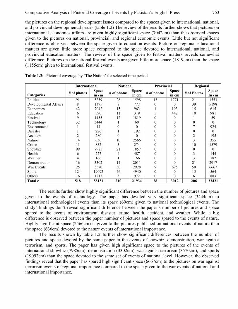
Comparative Analysis of Pictorial Coverage of Events by Pakistan’s English Press 753
the pictures on the regional development issues compared to the spaces given to international, national, and provincial developmental issues (table 1.2) The review of the results further shows that pictures on international economics affairs are given highly significant space (7042cm) than the observed spaces given to the pictures on national, provincial, and regional economic events. Little but not significant difference is observed between the space given to education events. Picture on regional educational matters are given little more space compared to the space devoted to international, national, and provincial education matters. The review of the space given to festival matters reveals somewhat difference. Pictures on the national festival events are given little more space (1819cm) than the space (1155cm) given to international festival events. Table 1.2: Pictorial coverage by ‘The Nation’ for selected time period
International National Provincial Regional
Categories # of photos Space in cm # of photos Space
in cm # of photos Space in cm # of Photos Space
In cm Politics 91 5259 28 1598 13 1771 21 1553 Developmental Affairs 8 1375 8 777 0 0 39 5198 Economics 42 7042 15 963 1 103 15 615 Education 6 590 11 319 5 442 10 981 Festival 9 1155 12 1819 0 0 1 59 Technology 32 3444 1 60 0 0 0 0 Environment 1 14 0 0 0 0 7 924 Disaster 1 226 1 192 0 0 0 0 Accident 2 280 0 0 0 0 2 195 Nature 14 636 10 2566 0 0 3 355 Crime 11 852 3 274 0 0 10 1579 Showbiz 99 7985 21 1857 0 0 0 0 Health 6 227 4 487 0 0 3 144 Weather 4 166 1 166 0 0 3 782 Demonstration 16 3302 14 2011 0 0 21 2917 War Events 25 3570 30 2928 9 695 50 6667 Sports 124 19092 46 4940 0 0 15 564 Others 16 1213 5 972 0 0 6 883 Total e 518 58131 210 21934 28 3012 206 23421
The results further show highly significant difference between the number of pictures and space
given to the events of technology. The paper has devoted very significant space (3444cm) to international technological events than its space (60cm) given to national technological events. The study’ findings don’t reveal significant difference between the paper’s number of pictures and space spared to the events of environment, disaster, crime, health, accident, and weather. While, a big difference is observed between the paper number of pictures and space spared to the events of nature. Highly significant space (2566cm) is given to the pictures published on national events of nature than the space (636cm) devoted to the nature events of international importance.
The results shown by table 1.2 further show significant differences between the number of pictures and space devoted by the same paper to the events of showbiz, demonstration, war against terrorism, and sports. The paper has given high significant space to the pictures of the events of international showbiz (7985cm), demonstration (3302cm), war against terrorism (3570cm), and sports (19092cm) than the space devoted to the same set of events of national level. However, the observed findings reveal that the paper has spared high significant space (6667cm) to the pictures on war against terrorism events of regional importance compared to the space given to the war events of national and international importance.
754 Muhammad Nawaz Mahsud, Muhammad Khalid and Firasat Jabeen
Conclusion
As it is evident from the figures of table 1.2 that daily ‘The Nation’ has significantly published more pictures (518) and spared more space (58131) in centimeter to the events of international importance than its number of pictures and space given to the events of national (210 pictures, 21934 space), provincial (28 pictures, 3012 space), and regional (206 pictures, 23421 space) importance.
The graphic presentation of the daily ‘Dawn’ shows that the paper has given more space to the pictures on the events of international and national importance compared to their space given to the events of provincial and regional importance (figure 1.1). Conversely, daily ‘The Nation’ space coverage devoted to the pictures published on the events of international, national, provincial, and regional matters of importance shows different position. The paper as shown by figure 1.2 has given significant space to the pictures on the events of regional importance than the events of international, national, and provincial importance. The comparison of both the papers number of pictures shows that daily ‘The Nation’ has published more pictures on international events than the national, provincial, and regional events (figure 1.3). While daily the ‘Dawn” has published more pictures on the events of international and national importance compared to its pictures on the events of provincial and regional importance (figure 1.4).
Figure 1.1: Dawn pictorial coverage
01000020000300004000050000
Internati
onal
Nationa
l
Provin
cial
Regiona
l
Figure 1.2: The Nation pictorial coverage
02000400060008000
10000
Internati
onal
Nationa
l
Provin
cial
Regiona
l
Figure 1.3: Picture Coverage by The Nation
518210
28
206 International
National
Provincial
Regional

Comparative Analysis of Pictorial Coverage of Events by Pakistan’s English Press 755
Figure 1.4: Picture coverage by Dawn
298
241
20
115International
National
Provincial
Regional
The empirical findings regarding both the dailies space coverage given to pictures published on the events for the whole three months period show that both the newspapers have spared significant space to the events of international importance than the events of national, provincial, and regional importance (figures 1.5 & 1.6). However, daily the ‘Dawn’ has given significantly more space to events of national level compared to the space given by daily ‘The Nation’ to the same events for same period.
Figure 1.5: Space coverage by The Nation
International49%
National27%
Regional21%
Province3%
Figure 1.6: Space coverage by Dawn
National35%
Province3%
Regional21% Internati
onal41%
Results of the study shown by table 1.3 illustrate the comparison of number of pictures and space given to the selected categories by both the papers for the whole stipulated period. As it is evident from the findings that daily ‘Dawn’ has significantly published more pictures and also spared significant space to developmental affairs, education, festival, disaster, accident, and crimes events of international, national, provincial, and regional importance compared to the number of pictures and space given by daily ‘The Nation’ to the same events for the same period. Conversely daily ‘The Nation’ published significantly more pictures and also given more space to the issues of politics, economics, technology, showbiz, health, war against terrorism, and sports of international, national, provincial, and regional importance. The results show no significant difference between both the papers’ coverage given to the events of environment, nature, weather, and others. In the light of the above findings it can be concluded that ‘The Nation’ has not published more pictures but also spared significant space to the listed set of issues compared to number of pictures and space devoted by ‘Dawn’ to the same events for the whole stipulated period.
756 Muhammad Nawaz Mahsud, Muhammad Khalid and Firasat Jabeen
Table 1.3: Both the papers’ Pictorial coverage Comparison
Dawn The Nation Categories # of photos Space in cm # of photos Space in cm Politics 40 4215 153 10181 Developmental Affairs 91 15437 55 7349 Economics 39 4300 73 8723 Education 37 4521 32 2332 Festival 36 7356 22 3033 Technology 15 2148 33 3504 Environment 9 1718 8 937 Disaster 5 9910 2 418 Accident 18 2243 4 475 Nature 27 4849 27 3557 Crime 28 5747 24 2705 Showbiz 56 6026 120 9842 Health 9 1163 13 858 Weather 8 1586 8 1115 Demonstration 53 10981 51 8230 War Events 65 11131 114 138510 Sports 108 16513 185 24597 Others 27 5230 27 3068 Total 712 112669 930 223 434
Conclusion The data in this review article mainly focused on many previous studies (Straubhaar & LaRose, 2004; Entman,1993; McQuail, 2005; and Bandura, 1986). Straubhaar & LaRose write that important events and figures can help to shape media content. Entman (1993) says that When information is supplied to news media by source then it arrives with a built in frame that suit the purpose of source and is unlikely to be purely objective. McQuail (2005) says that photographs are imagined to be powerful manipulators of human perception, precisely because they seem to give us a direct access to the real world. These have been selected to represent or reinforce the essence of a story, and to achieve widespread exposure in terms of the numbers of people who see the image. Bandura’s (1986) model posits four basic processes of social learning that occur in sequence: attention; retention; production; and motivation. Our attention is directed at media content of potential relevance to our lives and personal needs and interests.
Keeping in view the received empirical findings, first and perhaps most obviously, it can be noted that both the selected newspapers had spared significant space by almost all their pages to photographs on important events and figures of international, national, provincial, and regional importance. However, significant difference between the findings of the national leading dailies was observed. Daily the ‘Dawn’ had given more importance to developmental affairs, education, festival, disaster, accident, and crimes events compared to the space given by ‘The Nation’ to the same events. ‘The Nation’ conversely, had given significantly more space to the issues of politics, economics, technology, showbiz, health, war against terrorism, and sports than the space spared to the same events by daily ‘Dawn.’ The analytical review of the comparison of overall number of pictures and space by both the newspapers’ pages showed that international events and figures were given more importance than the events and figures national, provincial, and regional levels (ref. tables 1.1 and 1.2). It was also observed that both the papers had given significant importance to sports, showbiz, and war against terrorism’s events and personnel of international importance. A big difference was further traced out between Overall coverage of the papers had showed that ‘The Nation’ had published more number of pictures and spared significant space compared to the ‘Dawn’ number of pictures and space for the whole stipulated period (ref. table 1.3) This position had extended support to the research hypothesis

Comparative Analysis of Pictorial Coverage of Events by Pakistan’s English Press 757
that ‘The Nation publishes more pictures and gives more to the issues international, national, and regional importance than daily Dawn.’
The daily ‘Dawn’ had given more focus on issues of international and national importance, while ‘The Nation’ had paid little more focus on issues of regional importance (ref. figures 1.1 & 1.2). Finally the study’s results did not reveal significant difference between both the papers’ coverage given to the events of environment, nature, weather, and others. In the light of the above findings it can be concluded that ‘The Nation’ has not published more pictures but also spared significant space to compared to number of pictures and space by ‘Dawn’ for the whole stipulated period of three months. References [1] Bandura, A (1986). Social Foundations of thought and Actions: a Social Cognitive Theory.
Englewood Cliffs, NJ: Prentice-Hall. [2] Chaiken, S., Liberman, A., & Eagly. A.H (1989). “Heuristic and systematic within and Beyond
The Persuation Context”, in J. Bargh (ed.), Unintended Thought, pp. 212-252, New York: Guilford Press.
[3] Eagly, A.H., & Chaiken, S (1993). The Psychology of Attitudes, Fort Worth, TX: Harcourt, Brace, and Movanovich.
[4] Entman, R.M (1993). ‘Framing: Towards Clarification of a Fractured Paradigm’, Journal of Communication, 43(4): 51-8. http://www.clir.Org/pubs/reports/ostrow/pub71.htm/.
[5] Evans, H. (1978) Pictures on a Page, Heinemann, p. 216. [6] Evans, J (1999). ‘cultures of the visual’, in J. Evans and S. Hall (eds), Visual culture: a Reader,
(London: sage) p. 12. [7] Fiske, S.T., & Pavelchak, M.A (1986). “Category-based versus Piecemeal-based Affective
Responses: Development in Schematriggered Affect”. In R.M. Sorrentino & E.t. Higgings (eds.), Handbook of Motivation and Cognition: Foundation of Social Behaviour, New York: Guilford Press pp. 167-203,
[8] Friend, C., Challenger, D., & McAdams, K.C (2005). Contemporary Editing (The McGraw-Hill) pp.323-5.
[9] Frost, Chris (2003). Designing for newspapers and magazines. pp. 01, 02, 03, 115, 117, and 127.
[10] Goldsmith, A. (1979) The Camera and Its images (Ridge Press/Newsweek Books) pp. 166-7. [11] Greenwald, A.G (1968). “Cognitive Learning, Cognitive Response to Persuation, and Attitude
Change”, in A. Greenwald, t. Ostrom (Eds.) Psychological foundations of attitudes, New York Academic Press, pp. 147-170,
[12] Harrower, Tim (2002). The Newspaper Designer’s Handbook (McGraw-Hill), p. 4. [13] Hasan, Mehdi and Khursheed, A. S (1987). Journalism for All (Etisam Publishers, Lahore), pp.
185, 186. [14] Hansen, A., Siman, C. Ralph, N. & Chris, N (1998). Mass Communication Research Methods,
Palgrave, New York, N. Y. 10010. [15] McQuail, Denis (2005). Mass Communication Theory (Vistaar Publications, New Delhi), pp.
348-49. [16] McQuail, D, & Wendahl, S (1993). Communication Models; for the Study of Mass
Communication. (3rd Ed.) New York: Longman Publishing. [17] McLuhan, Marshall (2002). Understanding Media (TJ international Ltd, Padstow, Cornwall,
Great Britain), pp. 204, 206, 210, 214, 217, 218, 219. [18] Ostrow. S.E (1998). Digitizing Historical Pictorial Collections for the Internet.
http://www.clir.Org/pubs/reports/ostrow/pub71.htm/ [19] Palmerino, M., Linger, E., & McGillis, D (1984). “Attitudes and Attitude Change:
Mindlessness-mindfulness Perspective”, in J.R. Eisre (ed.) Attitudinal Judgment, New York: Springer-Verlag, pp. S179-195,

758 Muhammad Nawaz Mahsud, Muhammad Khalid and Firasat Jabeen
[20] Peterson, R.E. & Thurstone, L (1933). Motion Pictures and Social Attitudes of Children, New York: MacMillan.
[21] Petty, R.E. & Cacioppo, U.T (1981). Attitude and Persuation: Classic and Contemporary Approaches, Dubuque: Wm. C. Brown.
[22] Petty, R.E., Baker, S.M., & Gleicher, F (1991). “Attitudes and Drug Abuse Prevention: Implications of the Elaboration Likelihood Model of Persuation”, in L. Donohew, H.E. Syper, & W.J. Bukoski (eds.), Persuasive Communication and Drug Abuse Prevention, Hillsdale, NJ: Lawrence Erlbaum Associates, pp. 71-90.
[23] Petty, R.E, Unnava, R., & Strathman, A (1991). “Theories of Attitude Change”, in H. Kassarjain & T. Robertson (eds.), Handbook of Consumer Theory and Research, Englewood Cliffs, NJ: Prentice-Hall, pp. 241-280,
[24] Price, Stuart (1998). Media Studies, (Singapore through Addison Wesley Longman China Ltd), pp. 202-210, 213-14, and 217.
[25] Rothstein, A (1974). Photojournalism (Amphoto) pp. 15, 21. [26] Sontag, S (1978). On Photography (Penguin Books) pp. 3- 4, and 153-54. [27] Straubhaar,J & LaRose R (2004) Media Now:Understanding Media,Culture, and Technology
Thomson: Wadsworth. [28] Watson, J (1998). Media Communication. An Introduction to Theory and Process, London:
Macmillan Press Ltd. [29] Webster, C (1980). The New Photography (John Calder) pp. 172-73. [30] Wilder D.A. (1990). “Some Determinants of the Persuasive Power”.
www.shipshapewsiebiz.com/NewsRoom.asp-20k
European Journal of Scientific Research ISSN 1450-216X Vol.20 No.4 (2008), pp.759-771 © EuroJournals Publishing, Inc. 2008 http://www.eurojournals.com/ejsr.htm
Design Space Exploration of Regular NoC Architectures: A
Multi-Objective Evolutionary Algorithm Approach
Rabindra Ku. Jena Faculty of IT, Institute of Management Technology, Nagpur, India
E-mail: [email protected]
Musbah M. Aqel Faculty of IT, Middle East University for Graduate Studies
Ammam, Jordan E-mail: [email protected]
Gopal K. Sharma Department of IT
ABV-Indian Institute of Information Technology & Management, Gwalior, India E-mail: [email protected]
Prabhat K. Mahanti
Department of CSAS, University of New Brunswick, Saint John, Canada E-mail: [email protected]
Abstract
In this paper, we address the problem of topological mapping of intellectual properties (IPs) on the tile of a mesh-based NoC to minimize energy and maximum bandwidth requirement. As the stated problem is NP-hard in nature, we proposed a heuristic technique based on multi-objective genetic algorithm to obtain an optimal approximation of the pareto-optimal. We have considered “many-many” mapping between switch and cores (IPs) instead of “one-one” mapping. The evaluation performed on randomly generated benchmarks and a real application (a M-JPEG encoder), showed the efficiency, accuracy and scalability of our proposed approach. Keywords: NoC optimization, energy, performance, system level synthesis, Genetic
algorithm. 1. Introduction Network on Chip (NoC) has been proposed as a solution for the communication challenges like propagation delays, scalability, infeasibility of synchronous communication etc. in a nano scale regime (Zitzler and Thiele, 1999; Hu and Marculescu, 2003). To meet these challenges under the strong time-to-market pressure, it is essential to increase the reusability of components and system architectures in a plug and play fashion (Hu and Marculescu, 2003). Simultaneously, the volume of data and control traffic among the cores grows. So, it is essential to address the communication-architecture synthesis
Design Space Exploration of Regular NoC Architectures: A Multi-Objective Evolutionary Algorithm Approach 760 problem through mapping of cores onto the communication architecture (Lahiri, Raghunathan, and Dey, 2000).
Regular tile-based network-on-chip (NoC) architecture was proposed to mitigate these complex on-chip communication problems (Zitzler and Thiele, 1999; Jena et al, 2006; Hu and Marculescu, 2003). As shown in Figure 1, such a chip consists of a grid of regular tiles where each tile can be the resources/core like a general-purpose processor, a DSP, a memory subsystem, etc. A router is embedded within each tile with the objective of connecting it to its neighboring tiles. Thus, instead of routing design-specific global on-chip wires, the inter-tile communication can be achieved by routing packets.
Figure 1: Regular Tile-based NoC.
02
C C C
C C C
C C C
212 22
20
01 11 21
00 10 0
10 2
1
Three key concepts come together to make this tile-based architecture very promising: 1) Structured network wiring 2) Modularity 3) Standard interfaces More precisely, since the network wires are structured and wired beforehand, their electrical
parameters can be very well controlled and optimized. In turn, these controlled electrical parameters make it possible to use aggressively signaling circuits that help reduce the power dissipation and propagation delay significantly. Modularity and standard network interfaces facilitate reusability and interoperability of the modules. Moreover, since the network platform can be designed in advance and later reused directly with many applications, it makes sense to highly optimize this platform as its development cost can be easily amortized across many applications.
On the other hand, the regular tile-based architecture may lead to significant area overhead if applied to applications whose IPs’ sizes vary significantly. In order to achieve the best performance/ cost tradeoff, the designer needs to select the right NoC platform (e.g., the platform with the right size of tiles, routing strategies, buffer sizes, etc.) and further customize it according to the characteristics of the application under design. For most applications, the area cost overhead is fully compensated by the design time savings and performance gains because of the regular NoC architecture.
The advantages of using the regular NoC approach can be further increased if the IPs in the library are developed with regularity (in terms of size) taken into consideration as well. Moreover, partitioning the application with regularity in mind can also help in reducing the cost overhead. Finally, the region-based design (Kumar et al, 2002) can be used to further reduce the area overhead by embedding irregular regions inside the NoC, which can be insulated from the network. From the design perspective, given a target application described as a set of concurrent tasks which have been assigned and scheduled, to exploit the architecture in Figure 1. More precisely, in order to get the best energy/performance tradeoff, the designer needs to determine the topological placement of this IPs onto different tiles.
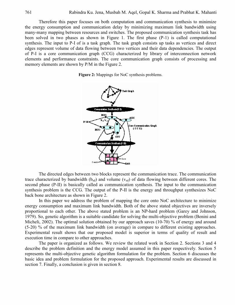
761 Rabindra Ku. Jena, Musbah M. Aqel, Gopal K. Sharma and Prabhat K. Mahanti
Therefore this paper focuses on both computation and communication synthesis to minimize the energy consumption and communication delay by minimizing maximum link bandwidth using many-many mapping between resources and switches. The proposed communication synthesis task has been solved in two phases as shown in Figure 1. The first phase (P-1) is called computational synthesis. The input to P-I of is a task graph. The task graph consists up tasks as vertices and direct edges represent volume of data flowing between two vertices and their data dependencies. The output of P-I is a core communication graph (CCG) characterized by library of interconnection network elements and performance constraints. The core communication graph consists of processing and memory elements are shown by P/M in the Figure 2.
Figure 2: Mappings for NoC synthesis problems.
The directed edges between two blocks represent the communication trace. The communication trace characterized by bandwidth (bsd) and volume (vsd) of data flowing between different cores. The second phase (P-II) is basically called as communication synthesis. The input to the communication synthesis problem is the CCG. The output of the P-II is the energy and throughput synthesizes NoC back bone architecture as shown in Figure 2.
In this paper we address the problem of mapping the core onto NoC architecture to minimize energy consumption and maximum link bandwidth. Both of the above stated objectives are inversely proportional to each other. The above stated problem is an NP-hard problem (Garey and Johnson, 1979). So, genetic algorithm is a suitable candidate for solving the multi-objective problem (Benini and Micheli, 2002). The optimal solution obtained by our approach saves (10-70) % of energy and around (5-20) % of the maximum link bandwidth (on average) in compare to different existing approaches. Experimental result shows that our proposed model is superior in terms of quality of result and execution time in compare to other approaches.
The paper is organized as follows. We review the related work in Section 2. Sections 3 and 4 describe the problem definition and the energy model assumed in this paper respectively. Section 5 represents the multi-objective genetic algorithm formulation for the problem. Section 6 discusses the basic idea and problem formulation for the proposed approach. Experimental results are discussed in section 7. Finally, a conclusion is given in section 8.

Design Space Exploration of Regular NoC Architectures: A Multi-Objective Evolutionary Algorithm Approach 762 2. Related Work The problem of synthesis in mesh-based NoC architectures has been addressed by different authors.(Hu and Marculescu, 2003) present a branch and bound algorithm for mapping IPs/cores on a mesh-based NoC architecture that minimizes the total amount of power consumed in communications. (De Micheli, 2004) addresses the problem under the bandwidth constraint with the aim of minimizing communication delay by exploiting the possibility of splitting traffic among various paths. (Lei and Kumar, 2003) present an approach that uses genetic algorithms to map an application on a mesh-based NoC architecture. The algorithm finds a mapping of the vertices of the task graph on the available cores so as to minimize the execution time. However these papers do not solve certain important issues. The first relates to the evaluation model used. In most of the approaches the exploration model decides the mapping to explore the design space without taking important dynamic effects of the system into consideration. Again in the above mentioned works, in fact, the application to be mapped is described using task graphs, as in (Lei and Kumar, 2003), or simple variations such as the core graph in (Murali and Micheli, 2004) or the application characterization graph (APCG) in (Hu and Marculescu, 2003). These formalisms do not, however, capture important dynamics of communication traffic. The second problem relates to the optimization method used. It refers in all cases to a single performance index (power in (Hu and Marculescu, 2003), performance in (Murali and Micheli, 2004; Lei and Kumar, 2003). So the optimization of one performance index may lead to unacceptable values for another performance index (e.g. high performance levels but unacceptable power consumption). Recently, (Jena and sharma, 2006) proposed a model that consider “many-many” mapping between core and tiles using multi-objective genetic algorithm. But they used core communication graph as the input to their model.
We therefore think that the problem of mapping can be more usefully solved in a multi-objective environment starting from the higher level of input (Task Graph) as compared to the model discussed in (Jena and sharma, 2006). The contribution we intend to make in this paper is to propose a multi-objective approach to solving the synthesis problem on a mesh-based NoC architecture, where we take the task graph as input. The approach will use evolutionary computing techniques based on genetic algorithm to explore the mapping space with the goal to optimize maximum link bandwidth and energy consumption (both computation and communication). 3. Problem Definition 3.1. A Task Graph (TG)
Is a digraph, G (V, E), where each vertex v Є V represent task and each edge e Є E is a weighted edge, where weight signifies the volume of data flowing through the edge. Every edge also represents the data dependency between the connecting vertices. 3.2. A Core Communication Graph (CCG)
Is a digraph, G(V, E), where each vertex v Є V represent core and e Є E is a communication edge having two attributes, denoted by bsd and vsd are the required bandwidth and total volume of communication respectively. 3.3. Communication Structure
The 2-D mesh communication architecture has been considered for its several desire properties like regularity, concurrent data transmission and controlled electrical parameters (Hu and Marculescu, 2003; Kumar et al, 2002). Figure 3 shows how a Tile (T) is binding with its surrounding switches(S) in a 2-D mesh NoC architecture. Each tile is a square surrounded by ‘4’ switches and links. A resource in a tile can be connected to maximum ‘4’ switches as shown in the Figure 3. Each switch is connected to

763 Rabindra Ku. Jena, Musbah M. Aqel, Gopal K. Sharma and Prabhat K. Mahanti
its neighboring switches via two unidirectional links. To prevent the packet loss due to the multiple packets approaching to the same output port, each switch has small buffers (registers) to temporarily store the packets. Each resource has ‘4’ Resource Network Interfaces (RNIs) to connect to the network via switches. RNIs are responsible for packetizing and depacketizing the communication data.
Figure 3: Communication Structure.
Core
Core Core
Core
NINI
NI NI
S4
S1 S2
S3
We implement static XY wormhole routing in this paper because: i) it is easy to implement in switch. ii) it doesn’t required packet ordering buffer at the destination. It is free of deadlock and live
lock (Banerjee et al, 2004; Murali and Micheli, 2004). 4. Energy Model Energy minimization is the one of the major challenging task in NoC design. In (Ye et al, 2002), Ye et al. first define the bit energy metric of a router as the energy consumed when a single bit of data goes through the router. In (Hu et al, 2003) modify the bit energy model so that it is suitable for 2D mesh NoC architecture. They derives mathematical expression for bit energy consume, when data transfer from switch ‘i’ to switch ‘j’ is given by
Ei,j bit = (hij+1) ESbit + hij ELbit (1) Where ESbit and ELbit are the energy consumed in the switches and links respectively. The
variable hij represent the number of links on the shortest path. As per the expression, the energy consumption is depend on the hop distance (hij) between switch ‘i’ and ‘j’ because ESbit and ELbit constant. Note ESbit is the energy consumption due to switches is depending on the number of ports in the switches. But in our case the total energy is the sum of communication and computation energy, i.e
E i, j bit = (hij + 1) ESbit + hij ELbit + ECom (2) EComp is the computational energy consumption. The following sections discuss the basic ideas
of problem formulation using multi-objective optimization paradigm. 5. Multi-Objective Optimization Definition A general multi-objective optimization problem is defined as: Minimize f (x) = (f1(x),….., fk(x)) subject to x Є X, where x represents a solution and X is a set of feasible solutions. The objective function vector f (x) maps a solution vector ‘x’ in decision space to a point in objective space.
In general, in a multi-objective optimization problem, it is not possible to find a single solution that minimizes all objectives, simultaneously. Therefore, one is interested to explore a set of solutions, called the pareto optimal set, which are not dominated by any other solution in the feasible set. The corresponding objective vectors of these Pareto optimal points, named efficient points, form the Pareto front on the objective space.

Design Space Exploration of Regular NoC Architectures: A Multi-Objective Evolutionary Algorithm Approach 764 Definition We say x dominates x* iff i Є 1,……,k
fi(x) ≤ fi(x*) and there exists at least one i Є 1,…., k such that fi(x) < fi(x*). The most traditional approach to solve a multi-objective optimization problem is to aggregate
the objectives into a single objective by using a weighting mean. However this approach has major drawbacks. It is not possible to locate the non-convex parts of the pareto front and it requires several consecutive runs of the optimization program with different weights. Recently, there has been an increasing interest in evolutionary multi-objective optimization. This is because of the fact that evolutionary algorithms (EAs) seem well-suited for this type of problems (Coello et al, 2002), as they deal simultaneously with a set of possible solutions called population. This allows us to find several members of the pareto optimal set in a single run of the algorithm. To solve the synthesis problem as discussed in section 4, we used the multi-objective genetic algorithm principle. 5.1. A Multi-Objective Genetic Algorithm
In order to deal with the multi-objective nature of NoC problem we have developed genetic algorithms at different phases in our model. The algorithm starts with a set of randomly generated solutions (population). The population’s size remains constant throughout the GA. Each iteration, solutions are selected, according to their fitness quality (ranking) to form new solutions (offspring). Offspring are generated through a reproduction process (Crossover, Mutation). In a multi-objective optimization, we are looking for all the solutions of best compromise, best solutions encountered over generations are fled into a secondary population called the “Pareto Archive”. In the selection process, solutions can be selected from this “Pareto Archive” (elitism). A part of the offspring solutions replace their parents according to the replacement strategy. In our study, we used elitist non-dominated sorting genetic algorithm NSGA-II by (Deb et al, 2002). The following section outlined the working principle of NSGA-II. 5.1.1. NSGA-II In this section we discuss how the elitist selection occurs in NSGA-II by the classification of the population into different fronts based on non dominated sorting ranks.
Figure 4: NAGA-II working principle.
In NSGA-II, as shown in Figure 4 the offspring population Qt is first created by using the parent population Pt. However, instead of finding the non dominated front of Qt only, first the two populations are combined together to form Rt of size 2N. Then a non – dominated sorting is used to classify the entire population Rt. Although this requires more effort compared to performing a non-dominating sorting on Qt alone, it allows a global non-domination check among the offspring and parent solutions. Once the non-dominated sorting is over, the new population is filled by solutions of different non-dominated fronts, one at a time. The filling starts with the best non-dominated front and

765 Rabindra Ku. Jena, Musbah M. Aqel, Gopal K. Sharma and Prabhat K. Mahanti
continues with solutions of the second non-dominated front, followed by the third non-dominated front and so on. Since the overall population size of Rt is 2N, not all fronts may be accommodated in N slots available in the new population. All fronts which could not be accommodated are simply deleted. When the last allowed front is being considered, there may exist more solutions in the last front than the remaining slots in the new population. This scenario is illustrated in Figure 4. Instead of arbitrarily discarding some members of the last front, it would be wise to use a niching strategy to choose the members of the last front, which reside in the least crowded region in that front. But we will not go into too much detail on that. For more details refer to (Deb, 2002). 6. Problem Formulation 6.1. Basic Idea
Like other algorithms in area of design automation, the algorithm of NoC communication architecture is a hard problem. Our attempt is to develop an algorithm that can give near optimal solution within reasonable time. Genetic algorithms have shown the potential to achieve the dual goal quite well (Jena et al, 2006; Lahiri et al, 2000; Srinivasan and Chatha, 2005).
As shown in Figure 5 and discussed in section 1, the problem is solved in two phases. The first phase (P-I) is basically a task assignment problem (TA-GA). The input to the problem is a TG. We assume that all the edge delays are a constant and equal to Average Edge Delay (AED) (Banerjee et al, 2004).The output of the first phase is a Core Communication Graph (CCG).
The main task of the second phase (P-II) is communication synthesis which basically deals with mapping of cores to the tiles of the NoC backbone using multi objective genetic algorithm. The next section discusses each phases in detail.
Figure 5: An overall design flow.
NoC Architecture DescriptionTask Graph
Task Assignment
Evaluation
TA-GA
Core Communication Graph
Core Tile Mapping
Evaluation
CTA-GA
Optimize NoC
P-I
P-II
Core Tile Switch Mapping
Evaluation
CTS-GA
6.1.1. Task Assignment Problem (TA-GA) Given a task graph TG with all edge delay are constant and equal to average edge delay and IPs with specifications matrix containing cost and computational energy. The main objectives of this phase are to assign the tasks from the task graph to the available IPs in order to:
(i) minimize the computational energy by reducing the power consumption.

Design Space Exploration of Regular NoC Architectures: A Multi-Objective Evolutionary Algorithm Approach 766
(ii) Minimize the total cost of the resources. The above said problem is a NP-hard multi-objective problem. We proposed a multi-objective genetic algorithm based on principle of NSGA-II as discussed in subsection 5.1.1. Generally, in genetic algorithm, the chromosome is the representation of solution to the
problem. In this case length of each chromosome is proportional to the number of nodes in a task graph. The i-th gene in the chromosome identifies the IP which is assigning the i-th node in the task graph. One example of chromosome encoding is given in Figure 5. Each gene (node in TG) in the chromosome contains an integer which represents a IP. Each IP is chosen from the list of permissible IPs for that task. As shown in the Figure 6 the task number ‘2’ in the task graph is assign to IP number ‘7’ which is chosen from set of IPs 7, 8, and 17. We consider a single point crossover to generate the offspring’s. As for mutation operation, we consider the mutation by substitution i.e. at a time a gene in a chromosome is chosen with some random probability and the value in the gene is substitute by one of the best permissible value (i.e the index value of an IP) for the gene. The aim is to assign more tasks to a particular IP to reduce the communication between IPs. (i.e., to minimize the number of IPs used for a task graph.)
Figure 6: Chromosome encoding for task assignment.
Chromosome
6.1.2. Core-Tile Mapping (CTM) After optimal assignment of tasks to the IPs, we get a Core Communication Graph (CCG) as shown in the Figure 5. The input to this mapping task CT-GA is a CCG and a structure of NoC back bone. In our case it is a n×m mesh. The objectives of the mapping are (i) to reduce the average communication distance between the cores (i.e., to reduce number of switches in the communication path). (ii) to maximize throughput(i.e., minimize the maximum link bandwidth) under the communication constraint. The task of CTM is solved in two steps:
(a) Core-Tile assignment (CTA-GA) (b) Core-Tile-Switch assignment (CTS-GA)
6.1.2.1. Core-tile Assignment (CTA-GA) Core-tile assignment is a multi-objective mapping which maps the cores from CCG to the tiles of the NoC structure. So the multi-objective genetic algorithm based on NSGA-II is a best candidate for the above said mapping problem. Here the chromosome is the representation of the solution to the problem, which in this case describe by the mapping.
The inputs to CTA-GA are the CCG and NoC backbone structure. In this case the Noc backbone is a 2D mesh. Each tile in mesh has an associated gene which identified the core mapped to the tile. In n×m mesh, for example the chromosome is formed by n×m genes. The i-th gene identified the core in the tiles in row (⎡(i/n)⎤) and column (i % n).
The crossover and mutation operators for this mapping have been defined suitably as follows: Crossover The crossover between two chromosomes C1 and C2 is generated a new chromosome C3 as follows. The dominant mapping between C1 and C2 is chosen. Its hot core (the hot core is the IP in CCG

767 Rabindra Ku. Jena, Musbah M. Aqel, Gopal K. Sharma and Prabhat K. Mahanti
required maximum communication) is remapped to a random tile in the mesh, resulting a new chromosome C3.
Algorithm Crossover (C1, C2) If (C1 dominate C2)
C3 = C1; else
C3 = C2; Swap (C3, Hot (C3), random(1,2,3,…….m×n)); Return (C3); The function Swap(C, i, j) exchange the i-th gene with j-th gene in the chromosome C.
Mutation: The mutation operator acts on a single chromosome (C) to obtained a muted chromosome C0 as follows. A tile Ts from chromosome C is chosen at random. Indicating the core in the tile Ts as cs and ct as the core with which cs communicates most frequently, cs is remapped on a tile adjacent to Ts so as to reduce the distance between cs and ct thus obtaining the mutated chromosome C0. Algorithm, given below describes the mutation operator. The RandomTile(C) function gives a tile chosen at random from chromosome C. The MaxCommunication(c) function gives the core, with which c communicates most frequently. The Row(C, T) and Col(C, T) functions respectively give the row and column of the tile T in chromosome C. Finally, the Upper, Lower, Left, Right(C, T) functions give the tile to the north, south, east and west of the tile T in chromosome C.
Mutate (C) Chromosome C0 = C; Tile Ts = Random Tile (C0); Core cs = C0-1(Ts); Core ct = MaxCommunication (cs); Tile Tt = C0 (ct); i f (Row(C0, Ts) < Row(C, Tt))
T 0s = Upper (C0, Ts); else if (Row(C0, Ts) > Row(C0, Tt))
T 0s = Lower(C0, Ts); else if (Col(C0, Ts) < Col(C0, Tt))
T 0s = Left(C0, Ts); else
T 0s = Right(C0, Ts); Swap (C0, Ts, T 0s); Return (C0);
6.1.2.2. Core-Tile-Switch assignment (CTS-GA) The CTS-GA is a crucial step in the whole optimization process. This step is followed by CTA-GA as discussed in the previous section. The input to CTS-GA is the best chromosomes from CTA-GA and CCG. The best chromosome derived from CTA-GA shows the efficient placement of core in the tiles of a 2D-mesh. As we discussed in section 1, our mapping is a many-many mapping from tiles to switches i.e. a tile can bind to more than one switch (maximum 4) and a switch can connected to more than one tiles (maximum 4). The aim of the many-many mapping is to reduce
(1) The hop distance between source and destination, and (2) The congestions at NI to increase the throughput.
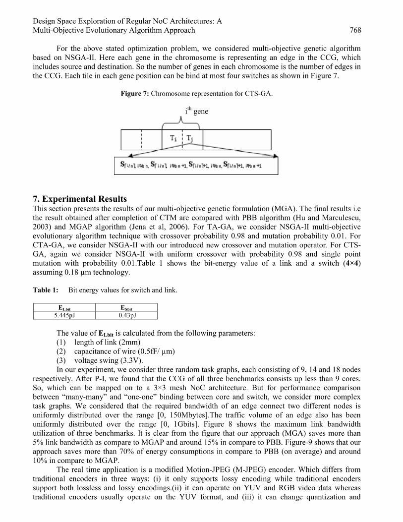
Design Space Exploration of Regular NoC Architectures: A Multi-Objective Evolutionary Algorithm Approach 768
For the above stated optimization problem, we considered multi-objective genetic algorithm based on NSGA-II. Here each gene in the chromosome is representing an edge in the CCG, which includes source and destination. So the number of genes in each chromosome is the number of edges in the CCG. Each tile in each gene position can be bind at most four switches as shown in Figure 7.
Figure 7: Chromosome representation for CTS-GA.
ith gene
7. Experimental Results This section presents the results of our multi-objective genetic formulation (MGA). The final results i.e the result obtained after completion of CTM are compared with PBB algorithm (Hu and Marculescu, 2003) and MGAP algorithm (Jena et al, 2006). For TA-GA, we consider NSGA-II multi-objective evolutionary algorithm technique with crossover probability 0.98 and mutation probability 0.01. For CTA-GA, we consider NSGA-II with our introduced new crossover and mutation operator. For CTS-GA, again we consider NSGA-II with uniform crossover with probability 0.98 and single point mutation with probability 0.01.Table 1 shows the bit-energy value of a link and a switch (4×4) assuming 0.18 µm technology. Table 1: Bit energy values for switch and link.
ELbit ESbit 5.445pJ 0.43pJ
The value of ELbit is calculated from the following parameters: (1) length of link (2mm) (2) capacitance of wire (0.5fF/ µm) (3) voltage swing (3.3V). In our experiment, we consider three random task graphs, each consisting of 9, 14 and 18 nodes
respectively. After P-I, we found that the CCG of all three benchmarks consists up less than 9 cores. So, which can be mapped on to a 3×3 mesh NoC architecture. But for performance comparison between “many-many” and “one-one” binding between core and switch, we consider more complex task graphs. We considered that the required bandwidth of an edge connect two different nodes is uniformly distributed over the range [0, 150Mbytes].The traffic volume of an edge also has been uniformly distributed over the range [0, 1Gbits]. Figure 8 shows the maximum link bandwidth utilization of three benchmarks. It is clear from the figure that our approach (MGA) saves more than 5% link bandwidth as compare to MGAP and around 15% in compare to PBB. Figure-9 shows that our approach saves more than 70% of energy consumptions in compare to PBB (on average) and around 10% in compare to MGAP.
The real time application is a modified Motion-JPEG (M-JPEG) encoder. Which differs from traditional encoders in three ways: (i) it only supports lossy encoding while traditional encoders support both lossless and lossy encodings.(ii) it can operate on YUV and RGB video data whereas traditional encoders usually operate on the YUV format, and (iii) it can change quantization and
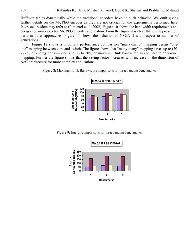
769 Rabindra Ku. Jena, Musbah M. Aqel, Gopal K. Sharma and Prabhat K. Mahanti
Huffman tables dynamically while the traditional encoders have no such behavior. We omit giving further details on the M-JPEG encoder as they are not crucial for the experiments performed here. Interested readers may refer to (Pimentel et al, 2002). Figure 10 shows the bandwidth requirements and energy consumptions for M-JPEG encoder application. From the figure it is clear that our approach out perform other approaches. Figure 11 shows the behavior of NSGA-II with respect to number of generations.
Figure 12 shows a important performance comparison “many-many” mapping versus “one-one” mapping between core and switch. The figure shows that “many-many” mapping saves up to (70-72) % of energy consumption and up to 20% of maximum link bandwidth in compare to “one-one” mapping. Further the figure shows that the saving factor increases with increase of the dimension of NoC architecture for more complex applications.
Figure 8: Maximum Link Bandwidth comparisons for three random benchmarks.
020406080
100120
1 2 3
Benchmarks
Max
imum
Lin
k B
andw
idth
(MB
/s)
MGA PBB MGAP
Figure 9: Energy comparisons for three random benchmarks.
050
100150200250
1 2 3
Benchmarks
Enar
gy
Con
sum
ptio
ns(m
J)
MGA PBB MGAP

Design Space Exploration of Regular NoC Architectures: A Multi-Objective Evolutionary Algorithm Approach 770
Figure 10: Maximum Link Bandwidth and Energy comparisons for M-JPEG.
00.20.40.60.8
1
Energy Max. LinkBandwidth
Performance MatricesN
orm
aliz
ed V
alue
s
MGA PBB MGAP
Figure 11: M-JPEG Encoder performance using NSGA-II.
Figure 12: ‘Many-Many’ Vs ‘One-One’ performance comparison.
8. Conclusion In this paper we have proposed a model for topological mapping of IPs/cores in a mesh-based NoC architecture with many- many mappings between core to switches. The approach uses heuristics based on multi-objective genetic algorithms (NSGA-II) to explore the mapping space and find the pareto mappings that optimize Maximum link bandwidth and performance and power consumption. The experiments carried out with randomly generated benchmarks and a real application (M-JPEG encoder system) confirms the efficiency, accuracy and scalability of the proposed approach. Future developments will mainly address the definition of more efficient genetic operators to improve the precision and convergence speed of the algorithm Evaluation will also be made of the possibility of

771 Rabindra Ku. Jena, Musbah M. Aqel, Gopal K. Sharma and Prabhat K. Mahanti
optimizing mapping by acting on other architectural parameters such as routing strategies, switch buffer sizes, etc. References [1] A. D. Pimentel, S. Polstra, F. Terpstra, A. W. van Halderen, J. E. Coffland, and L.
O.Hertzberger (2002) Towards efficient design space exploration of heterogeneous embedded media systems. E. Deprettere, J. Teich, and S. Vassiliadis, editors, Embedded Processor Design Challenges: Systems, Architectures, Modeling, and Simulation, volume 2268 of LNCS, Springer-Verlag, pp.7–73.
[2] C. A. Coello, D. A. Van Veldhuizen, and G. B. Lamont (2002) Evolutionary Algorithms for Solving Multi-Objective Problems. Kluwer Academic Publishers, New York.
[3] C. J. Glass and L. M. Ni (1992) The Turn Model for Adaptive Routing, Proc.19th Ann. Int’l Symp. Computer Architecture, pp. 278-287.
[4] Deb, K. (2002) Multi-Objective Optimization using Evolutionary Algorithms, John Wiley and Sons Ltd, pp. 245-253.
[5] E. Zitzler and L. Thiele (1999) Multi-objective evolutionary algorithms: A comparative case study and the strength pareto approach, IEEE Transactions on Evolutionary Computation, 4(3), pp.257–271.
[6] J. Hu and R. Marculescu (2003) Energy-aware mapping for tile-based NoC architectures under performance constraints, Asia & South Pacific Design Automation Conference.
[7] J. Hu and R. Marculescu (2003) Exploiting the Routing Flexibility for Energy/Performance Aware Mapping of Regular NoC Architectures, Proc. DATE’03, pp. 688-693.
[8] Jena R. K., Sharma, G.K, (2006) A multi-objective Optimization Model for Energy and Performance Aware Synthesis of NoC architecture, Proceedings of IP/SoC, Decmber 6-7, pp 477-482.
[9] K. Lahiri, A. Raghunathan, and S. Dey (2000) Efficient Exploration of the SoC Communication Architecture Design Space, Proc. IEEE/ACM ICCAD’00, pp. 424-430.
[10] K. Srinivasan and Karam S. Chatha (2005) ISIS: A Genetic Algorithm based Technique for Custom On-Chip Interconnection Network Synthesis, Proceedings of the 18th International Conference on VLSI Design (VLSID’05).
[11] Luca Benini and Giovanni De Micheli (2002) Networks on Chips: A New SoC Paradigm, IEEE Computer, pp. 70–78.
[12] M. R. Garey and D. S. Johnson (1979) Intractability: a guide to the theory of NP-completeness, Freeman and Company.
[13] N. Banerjee, P. Vellanki, and K. S. Chatha (2004) A power and performance model for network-on-chip architectures, Design, Automation and Test in Europe, pp. 1250–1255.
[14] S. Kumar et al. (2002) A Network on Chip Architecture and Design Methodology, Proc. ISVLSI’02, April 2002, pp. 105-112.
[15] S. Murali and G. D. Micheli (2004) Bandwidth-constrained mapping of cores onto NoC architectures, Design, Automation, and Test, Europe IEEE Computer Society, pp. 896–901.
[16] T. Lei and S. Kumar (2003) A two-step genetic algorithm for mapping task graphs to a network on chip architecture, Euro micro Symposium on Digital Systems Design, Sept. 1–6.
[17] T. T. Ye, L. Benini, and G. D. Micheli (2002) Analysis of Power Consumption on Switch Fabrics in Network Routers, Proc. DAC’02, pp.524-529.
[18] William J. Dally and Brian Towles (2002) Route Packet, Not Wires: On-Chip Interconnection Networks, Proceedings of DAC.
European Journal of Scientific Research ISSN 1450-216X Vol.20 No.4 (2008), pp.772-787 © EuroJournals Publishing, Inc. 2008 http://www.eurojournals.com/ejsr.htm
Etude Comparative des Méthodes D’évaluation de la
Vulnérabilité à la Pollution des Aquifères en Milieu Poreux: Application Aux Eaux Souterraines du
District D’abidjan (Sud de la Côte D’ivoire)
Kouamé Kan Jean Laboratoire des Sciences et Techniques de l’eau et de l’Environnement (LSTEE)
UFR des Sciences de la Terre et des Ressources Minières Université de Cocody Abidjan (UCA), 22 BP 582 Abidjan 22
Jourda Jean Patrice
Laboratoire des Sciences et Techniques de l’eau et de l’Environnement (LSTEE) UFR des Sciences de la Terre et des Ressources Minières
Université de Cocody Abidjan (UCA), 22 BP 582 Abidjan 22 Centre Universitaire de Recherche et d’Application en Télédétection (CURAT)
UFR des Sciences de la Terre et des Ressources Minières, 22 BP 801 Abidjan 22
Adja Miessan Germain Laboratoire des Sciences et Techniques de l’eau et de l’Environnement (LSTEE)
UFR des Sciences de la Terre et des Ressources Minières Université de Cocody Abidjan (UCA), 22 BP 582 Abidjan 22
Deh Serges Kouakou
Laboratoire des Sciences et Techniques de l’eau et de l’Environnement (LSTEE) UFR des Sciences de la Terre et des Ressources Minières
Université de Cocody Abidjan (UCA), 22 BP 582 Abidjan 22
Anani Abenan Tawa Laboratoire des Sciences et Techniques de l’eau et de l’Environnement (LSTEE)
UFR des Sciences de la Terre et des Ressources Minières Université de Cocody Abidjan (UCA), 22 BP 582 Abidjan 22
Effini Adiow Thérèse
Laboratoire des Sciences et Techniques de l’eau et de l’Environnement (LSTEE) UFR des Sciences de la Terre et des Ressources Minières
Université de Cocody Abidjan (UCA), 22 BP 582 Abidjan 22
Biémi Jean Laboratoire des Sciences et Techniques de l’eau et de l’Environnement (LSTEE)
UFR des Sciences de la Terre et des Ressources Minières Université de Cocody Abidjan (UCA), 22 BP 582 Abidjan 22
Centre Universitaire de Recherche et d’Application en Télédétection (CURAT) UFR des Sciences de la Terre et des Ressources Minières, 22 BP 801 Abidjan 22

Etude Comparative des Méthodes D’évaluation de la Vulnérabilité à la Pollution des Aquifères en Milieu Poreux: 773
Abstract Supply drinking water of Abidjan District population is dependent of groundwater
and water quality is unceasingly threatened to various potential sources of pollution. This study aims to determine the most relevant method in the evaluation of Abidjan District groundwater vulnerability to pollution in order to protect them. Application of DRASTIC and GOD methods in this study allowed evaluating intrinsic vulnerability of groundwater to pollution of Abidjan District. A comparative study starting from Kappa test and statistical analysis of surfaces, were thus carried out. Statistical analysis of different vulnerability maps to pollution reveals that vulnerability is concentrated between "moderate and high” classes with 88.37 and 88.18 percent of study area respectively for DRASTIC and GOD methods. Comparative study showed that DRASTIC and GOD methods have a moderate agreement (Kappa coefficient is 41 percent) but GOD tends to overestimate the vulnerability of an index compared to DRASTIC. Also, vulnerability map to pollution resulting from DRASTIC method was retained for the evaluation of Abidjan District groundwater vulnerability to pollution. Keywords: Evaluation, Vulnerability, groundwater Pollution, Abidjan District, Côte
d'Ivoire 1. Introduction La protection des eaux souterraines est une question de plus en plus préoccupante tant au niveau de l’exploitation de la ressource qu’à celui des impacts sur la santé humaine. La préservation de la qualité de l’eau souterraine est d’autant plus importante du fait que cette ressource, une fois contaminée, est difficile à être réhabilitée (Banton et Bangoy, 1997). De plus, certains contaminants peuvent persister durant des dizaines ou des centaines d’années, du fait des processus d’atténuation (adsorption, dégradation) limités en milieu aquifère (Banton et Bangoy, 1997). Le problème devient plus grave pour les pays à ressources en eau limitées comme c’est le cas du District d’Abidjan où la population est tributaire des eaux souterraines (Jourda et al., 2003). La qualité de cette eau est sans cesse menacée par les diverses sources potentielles de pollution du District d’Abidjan (Kouadio et al., 1998; Jourda et al., 2006a). L'insuffisance ou l'absence de stations d'épuration dans les zones d'activités domestiques et industrielles permet d'appréhender l'ampleur de la catastrophe qui menace les eaux souterraines (Jourda et al., 2006a; Kouamé, 2007). Ces carences font que, le plus souvent, la pollution de ces eaux est constatée après ses méfaits, c'est-à-dire après qu'elle ait migré de sa zone initiale et atteint par recharge les eaux souterraines. Etant donné les coûts importants engendrés par la restauration des aquifères contaminés, la protection des eaux souterraines du District d’Abidjan devient alors primordiale afin de sauvegarder, à moyen et à long terme, sa qualité (Jourda et al., 2006b). Une des approches d’aide à la protection et à la prévention contre la pollution des eaux souterraines est la cartographie des zones vulnérables à la pollution (Champagne et Chapuis, 1993). Cette étude a été entreprise dans le but d'identifier les zones à haut risque de contamination, indépendamment du type de polluant et de déterminer la méthode qui permet de mieux évaluer la vulnérabilité. Elle devrait en principe conditionner les plans d'occupation des sols ou, du moins, permettre de cibler les zones où des mesures rigoureuses de protection devraient être adoptées. 2. Présentation de la Zone D’étude Le District d’Abidjan (Figure 1) sur lequel porte cette étude, est situé au Sud de la Côte d’Ivoire et regroupe les dix communes de la ville d’Abidjan plus trois Sous-préfectures (Bingerville, Songon et Anyama). D’une superficie de 2 119 Km2 avec un taux de croissance de 3,7% et une densité de
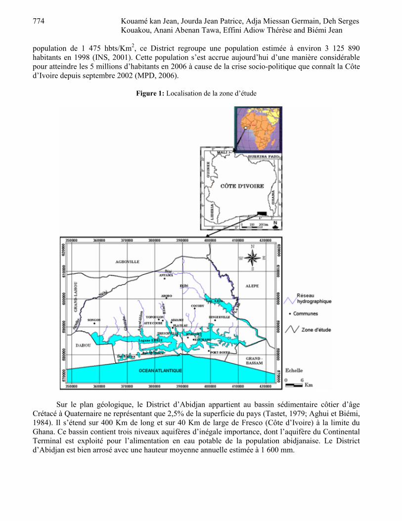
774 Kouamé kan Jean, Jourda Jean Patrice, Adja Miessan Germain, Deh Serges Kouakou, Anani Abenan Tawa, Effini Adiow Thérèse and Biémi Jean
population de 1 475 hbts/Km2, ce District regroupe une population estimée à environ 3 125 890 habitants en 1998 (INS, 2001). Cette population s’est accrue aujourd’hui d’une manière considérable pour atteindre les 5 millions d’habitants en 2006 à cause de la crise socio-politique que connaît la Côte d’Ivoire depuis septembre 2002 (MPD, 2006).
Figure 1: Localisation de la zone d’étude
Sur le plan géologique, le District d’Abidjan appartient au bassin sédimentaire côtier d’âge Crétacé à Quaternaire ne représentant que 2,5% de la superficie du pays (Tastet, 1979; Aghui et Biémi, 1984). Il s’étend sur 400 Km de long et sur 40 Km de large de Fresco (Côte d’Ivoire) à la limite du Ghana. Ce bassin contient trois niveaux aquifères d’inégale importance, dont l’aquifère du Continental Terminal est exploité pour l’alimentation en eau potable de la population abidjanaise. Le District d’Abidjan est bien arrosé avec une hauteur moyenne annuelle estimée à 1 600 mm.

Etude Comparative des Méthodes D’évaluation de la Vulnérabilité à la Pollution des Aquifères en Milieu Poreux: 775
3. Matériel et Méthodes 3.1. Matériel
Pour l’élaboration des paramètres physiques de la nappe, les données suivantes de la zone d’étude ont été utilisées:
• les cartes géologique et géotechnique de la région d’Abidjan; • les cartes topographiques; • la carte du réseau hydrographique; • les données de pluie, de température, de piézomètre et de puits; • les coupes de forage. Pour le traitement et l’élaboration des couches, les logiciels MapInfo 5.0, ArcView 3.2 et EVC
ont été utilisés. Toutes les cartes utilisées sont au 1/50 000 et ont été scannées et numérisées sous MapInfo dans
le système de coordonnées UTM WGS 84, zone 30, hémisphère nord. 3.2. Méthodes
L’évaluation de la vulnérabilité intrinsèque a été réalisée à partir de deux méthodes. Il s’agit des méthodes DRASTIC et GOD. Méthode DRASTIC La méthode DRASTIC, développée en 1987 aux Etats-Unis par l’Agence américaine de la Protection de l’Environnement (EPA), permet de cartographier les zones vulnérables à la pollution (Aller et al., 1987; Vrba et Zaporozec, 1994). C’est une méthode standardisée d’évaluation et de cartographie de la vulnérabilité des eaux souterraines indépendamment du type de polluant. Elle prend en compte la majeure partie des facteurs hydrogéologiques qui affectent et contrôlent l’écoulement des eaux souterraines (Mohamed, 2001). Elle permet de visualiser le degré relatif de vulnérabilité des eaux souterraines de la zone d’étude, car basée sur sept paramètres de vulnérabilité (Bézélgues et al., 2002). Ce sont:
• la profondeur de l’eau (D); • la recharge efficace (R); • les matériaux de l’aquifère (A); • le type de sol (S); • la topographie ou la pente (T); • l’impact de la zone non saturée ou zone aérée (I); • la perméabilité ou la conductivité hydraulique de l’aquifère (C). L’évaluation de la vulnérabilité par la méthode DRASTIC s’effectue par le calcul de l’Indice
DRASTIC (ID) selon l’équation (1) où les indices c et p désignent respectivement la "cote"et le "poids" du paramètre.
CpCcIpIcTpTcSpScApAcRpRcDpDcID ×+×+×+×+×+×+×= (1) L’indice (ID) ainsi calculé représente une mesure du niveau de risque de contamination de
l’unité hydrogéologique à laquelle il se rattache. Ce risque augmente avec la valeur de l’indice. Après le calcul de l’indice (IDRASTIC), on fait correspondre des classes de vulnérabilité aux différentes plages d’indices calculés. Les classes proposées par la méthode DRASTIC sont consignées dans le table I-.

776 Kouamé kan Jean, Jourda Jean Patrice, Adja Miessan Germain, Deh Serges Kouakou, Anani Abenan Tawa, Effini Adiow Thérèse and Biémi Jean
Table I: Intervalles des valeurs des ID et classes correspondantes (Aller et al., 1987)
Intervalles Classe DRASTIC 23 – 80 Vulnérabilité très faible 80 – 100 Vulnérabilité faible 100 – 140 Vulnérabilité modérée 140 – 180 Vulnérabilité forte 180 – 226 Vulnérabilité extrême
La classification de la carte des indices en fonction des plages définies par la méthode, a permis
d’élaborer la carte de vulnérabilité à la pollution des eaux souterraines du District d’Abidjan. Méthode GOD Comme la méthode DRASTIC, GOD est une méthode des systèmes paramétriques, conçue en Angleterre en 1987 par Foster. Elle utilise également une approche empirique où la vulnérabilité des aquifères est définie en fonction de l’inaccessibilité de la zone saturée, au sens de la pénétration du polluant, et de la capacité d’atténuation que présente la couche sus-jacente à la zone saturée. La méthode GOD permet de réaliser une estimation rapide de la vulnérabilité d’un aquifère (Bézelgues et al., 2002). Elle diffère de la méthode DRASTIC dans le sens où le nombre de paramètres de vulnérabilité n’est que de trois pour l’évaluation de la vulnérabilité intrinsèque des aquifères. Le premier réside dans l’identification du type d’aquifère en fonction de son degré de confinement (Ca). Le deuxième correspond à la profondeur à la nappe (Cd) et le troisième est défini par la lithologie de l’aquifère (Cl) (Murat et al., 2003). L’indice GOD (IGOD) qui permet d’évaluer la vulnérabilité de l’aquifère à la pollution est obtenu par la multiplication de ces trois paramètres. L’indice GOD (IGOD) se détermine selon l’équation (2), avec C, la cote du paramètre (Murat et al., 2000):
CdClCaIG ××= (2) Après le calcul de l’indice, on fait correspondre des classes de vulnérabilité aux différentes
plages d’indices obtenues. D’une manière générale, les indices GOD sont répartis en cinq classes de vulnérabilité allant du "très faible" à "extrême"(Table II). Le degré de vulnérabilité augmente avec l’indice GOD. Table II: Intervalles des valeurs de IGOD et classes correspondantes (Murat et al., 2003)
Intervalle Classe GOD 0 – 0,1 Vulnérabilité très faible 0,1 – 0,3 Vulnérabilité faible 0,3 – 0,5 Vulnérabilité modérée 0,5 – 0,7 Vulnérabilité forte 0,7 – 1 Vulnérabilité extrême
Les différentes classes des indices de vulnérabilité GOD permettent l’élaboration de la carte de
vulnérabilité à la pollution des eaux souterraines au niveau du District d’Abidjan. Les cartes de vulnérabilité étant des outils importants d’aide à la prise de décision en matière de
gestion d’aménagement du territoire, elles doivent refléter la réalité d’où la nécessité de leur validité. Méthode de validation des méthodes de cartographie de la de vulnérabilité à la pollution La détérioration de la qualité de l’eau souterraine est appréciée par mesures des paramètres physico-chimiques et bactériologiques. Plusieurs auteurs (Isabel et al., 1990; Champagne et Chapuis, 1993; Mohamed, 2001; Jourda et al., 2003; Kouamé, 2003; Douagui, 2004; Fofana, 2005; Jourda, 2005; Jourda et al., 2005; Anani, 2006 et Jourda et al., 2006b) ont vérifié la validité des méthodes d’évaluation de la vulnérabilité à la pollution en se basant sur des données chimiques des eaux

Etude Comparative des Méthodes D’évaluation de la Vulnérabilité à la Pollution des Aquifères en Milieu Poreux: 777
souterraines. Dans la validation des cartes de vulnérabilité, les zones réellement contaminées doivent correspondre à celles où les indices de vulnérabilité sont les plus élevés. Une zone vulnérable peut également avoir un faible indice de vulnérabilité du fait que la notion de vulnérabilité n’est pas synonyme d’une pollution actuelle, mais plutôt d’une prédisposition de ces zones à une contamination éventuelle, si rien n’est entrepris pour les protéger (Kouamé, 2007). La validation des cartes de vulnérabilité a porté sur l’analyse du taux de nitrates contenu dans les eaux souterraines du District d’Abidjan. Les données de nitrate utilisées couvrent que la ville d’Abidjan et datent de 2001.
Une étude comparative des deux méthodes utilisées s’avère indispensable en vue de déterminer celle qui permet de mieux évaluer la vulnérabilité à la pollution des eaux souterraines du District d’Abidjan. Etude comparative des méthodes d’évaluation de la vulnérabilité Dans cette étude comparative, la méthode DRASTIC est celle qui servira de référence pour déterminer les variations d’évaluation de la vulnérabilité. Deux méthodes statistiques ont été utilisées pour faire cette comparaison:
• le test de conformité (coefficient de kappa) Le coefficient de Kappa (K) représente l'indice statistique qui mesure le degré de concordance
ou d’accord d'une évaluation entre deux ou plusieurs méthodes ayant à juger un même phénomène. Un guide d'interprétation, suggéré par Landis et Koch (1977), permet d’apprécier le degré d’accord en fonction de la valeur observée du coefficient Kappa.
• l’analyse statistique des surfaces L’analyse statistique des surfaces permettra de savoir si la méthode GOD sous-évalue, sur-
évalue ou évaluation identiquement la vulnérabilité par rapport à la méthode DRASTIC prise comme référence. Les données utilisées par ces méthodes de comparaison sont les deux cartes de vulnérabilité produites par les méthodes DRASTIC et GOD, et le nombre de pixels par classe de vulnérabilité. 4. Résultats et Discussion L’établissement des différents paramètres et leur combinaison ont permis de réaliser les cartes de vulnérabilité à la pollution selon les deux méthodes. 4.1. Carte de vulnérabilité à la pollution à partir de la méthode DRASTIC
Dans le cas de la méthode DRASTIC, les valeurs des indices DRASTIC (IDRASTIC) calculés oscillent entre 113 et 192. La vulnérabilité à la pollution augmente avec l’indice obtenu. En tenant compte du fait que les valeurs limites des intervalles des indices DRASTIC sont relatives, une autre classification adaptée à l’étude a donc été effectuée. Cette autre classification permet de fixer les limites des intervalles des indices calculés et de faire correspondre des classes de vulnérabilité à ces indices. Ce fut le cas des travaux réalisés par Lynch et al. (1993), Lobo-Ferreira et al. (1995), Navalur et Engel (1997), Murat et al. (2000), Kimmeier (2001), Mohamed (2001), Murat et al. (2003), Jourda (2005) et Kouamé (2007). Les classes de vulnérabilité élaborées à partir de ces travaux en tenant compte des valeurs des IDRASTIC, varient entre "Faible” et "Très forte”, et sont résumées dans le tableau III. Une telle classification tient compte des valeurs minimum et maximum d’indices obtenus et non des classes standard définies par Aller et al. (1987).
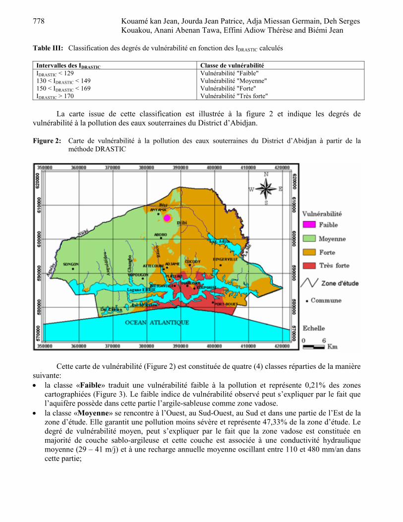
778 Kouamé kan Jean, Jourda Jean Patrice, Adja Miessan Germain, Deh Serges Kouakou, Anani Abenan Tawa, Effini Adiow Thérèse and Biémi Jean
Table III: Classification des degrés de vulnérabilité en fonction des IDRASTIC calculés
Intervalles des IDRASTIC Classe de vulnérabilité IDRASTIC < 129 Vulnérabilité "Faible" 130 < IDRASTIC < 149 Vulnérabilité "Moyenne" 150 < IDRASTIC < 169 Vulnérabilité "Forte" IDRASTIC > 170 Vulnérabilité "Très forte"
La carte issue de cette classification est illustrée à la figure 2 et indique les degrés de
vulnérabilité à la pollution des eaux souterraines du District d’Abidjan. Figure 2: Carte de vulnérabilité à la pollution des eaux souterraines du District d’Abidjan à partir de la
méthode DRASTIC
Cette carte de vulnérabilité (Figure 2) est constituée de quatre (4) classes réparties de la manière suivante: • la classe «Faible» traduit une vulnérabilité faible à la pollution et représente 0,21% des zones
cartographiées (Figure 3). Le faible indice de vulnérabilité observé peut s’expliquer par le fait que l’aquifère possède dans cette partie l’argile-sableuse comme zone vadose.
• la classe «Moyenne» se rencontre à l’Ouest, au Sud-Ouest, au Sud et dans une partie de l’Est de la zone d’étude. Elle garantit une pollution moins sévère et représente 47,33% de la zone d’étude. Le degré de vulnérabilité moyen, peut s’expliquer par le fait que la zone vadose est constituée en majorité de couche sablo-argileuse et cette couche est associée à une conductivité hydraulique moyenne (29 – 41 m/j) et à une recharge annuelle moyenne oscillant entre 110 et 480 mm/an dans cette partie;
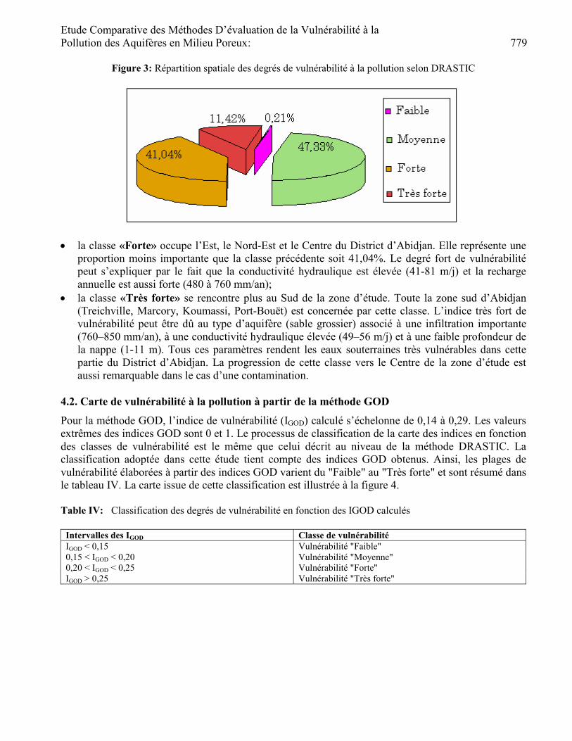
Etude Comparative des Méthodes D’évaluation de la Vulnérabilité à la Pollution des Aquifères en Milieu Poreux: 779
Figure 3: Répartition spatiale des degrés de vulnérabilité à la pollution selon DRASTIC
• la classe «Forte» occupe l’Est, le Nord-Est et le Centre du District d’Abidjan. Elle représente une
proportion moins importante que la classe précédente soit 41,04%. Le degré fort de vulnérabilité peut s’expliquer par le fait que la conductivité hydraulique est élevée (41-81 m/j) et la recharge annuelle est aussi forte (480 à 760 mm/an);
• la classe «Très forte» se rencontre plus au Sud de la zone d’étude. Toute la zone sud d’Abidjan (Treichville, Marcory, Koumassi, Port-Bouët) est concernée par cette classe. L’indice très fort de vulnérabilité peut être dû au type d’aquifère (sable grossier) associé à une infiltration importante (760–850 mm/an), à une conductivité hydraulique élevée (49–56 m/j) et à une faible profondeur de la nappe (1-11 m). Tous ces paramètres rendent les eaux souterraines très vulnérables dans cette partie du District d’Abidjan. La progression de cette classe vers le Centre de la zone d’étude est aussi remarquable dans le cas d’une contamination.
4.2. Carte de vulnérabilité à la pollution à partir de la méthode GOD
Pour la méthode GOD, l’indice de vulnérabilité (IGOD) calculé s’échelonne de 0,14 à 0,29. Les valeurs extrêmes des indices GOD sont 0 et 1. Le processus de classification de la carte des indices en fonction des classes de vulnérabilité est le même que celui décrit au niveau de la méthode DRASTIC. La classification adoptée dans cette étude tient compte des indices GOD obtenus. Ainsi, les plages de vulnérabilité élaborées à partir des indices GOD varient du "Faible" au "Très forte" et sont résumé dans le tableau IV. La carte issue de cette classification est illustrée à la figure 4. Table IV: Classification des degrés de vulnérabilité en fonction des IGOD calculés
Intervalles des IGOD Classe de vulnérabilité IGOD < 0,15 Vulnérabilité "Faible" 0,15 < IGOD < 0,20 Vulnérabilité "Moyenne" 0,20 < IGOD < 0,25 Vulnérabilité "Forte" IGOD > 0,25 Vulnérabilité "Très forte"
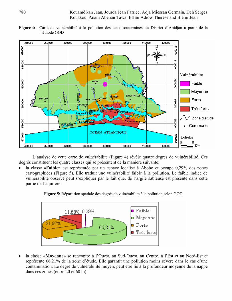
780 Kouamé kan Jean, Jourda Jean Patrice, Adja Miessan Germain, Deh Serges Kouakou, Anani Abenan Tawa, Effini Adiow Thérèse and Biémi Jean
Figure 4: Carte de vulnérabilité à la pollution des eaux souterraines du District d’Abidjan à partir de la
méthode GOD
L’analyse de cette carte de vulnérabilité (Figure 4) révèle quatre degrés de vulnérabilité. Ces degrés constituent les quatre classes qui se présentent de la manière suivante: • la classe «Faible» est représentée par un espace localisé à Abobo et occupe 0,29% des zones
cartographiées (Figure 5). Elle traduit une vulnérabilité faible à la pollution. Le faible indice de vulnérabilité observé peut s’expliquer par le fait que, de l’argile sableuse est présente dans cette partie de l’aquifère.
Figure 5: Répartition spatiale des degrés de vulnérabilité à la pollution selon GOD
• la classe «Moyenne» se rencontre à l’Ouest, au Sud-Ouest, au Centre, à l’Est et au Nord-Est et
représente 66,21% de la zone d’étude. Elle garantit une pollution moins sévère dans le cas d’une contamination. Le degré de vulnérabilité moyen, peut être lié à la profondeur moyenne de la nappe dans ces zones (entre 20 et 60 m);
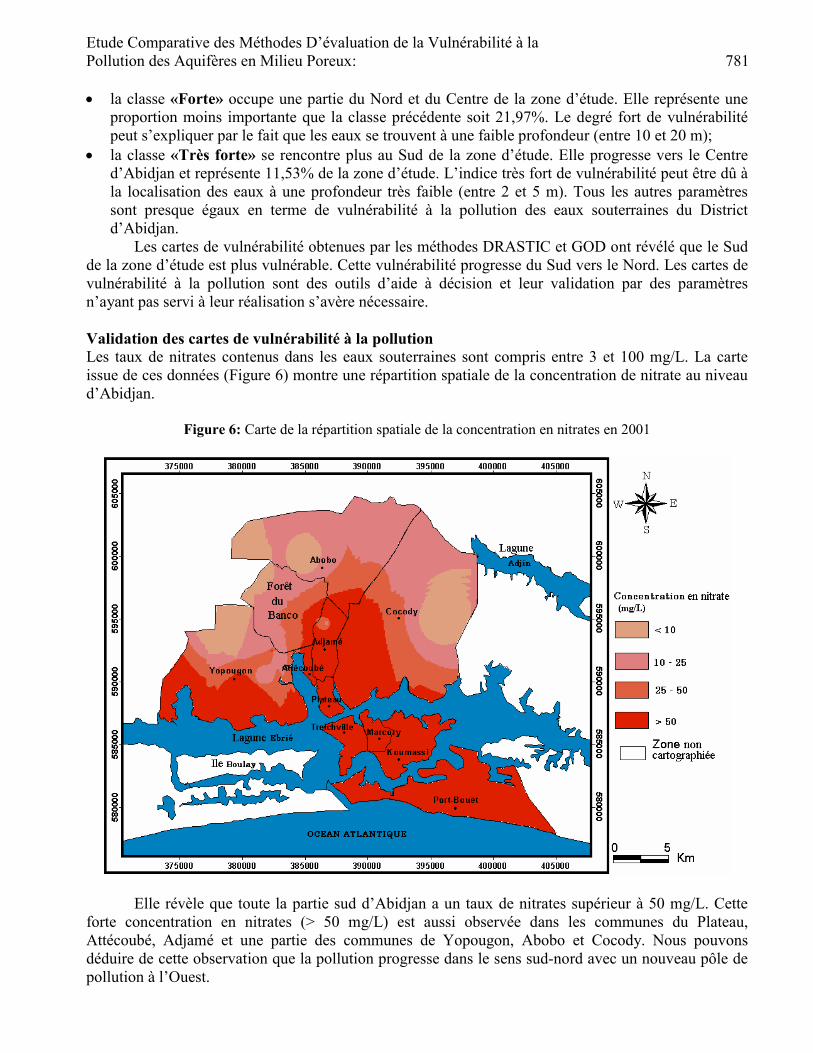
Etude Comparative des Méthodes D’évaluation de la Vulnérabilité à la Pollution des Aquifères en Milieu Poreux: 781
• la classe «Forte» occupe une partie du Nord et du Centre de la zone d’étude. Elle représente une proportion moins importante que la classe précédente soit 21,97%. Le degré fort de vulnérabilité peut s’expliquer par le fait que les eaux se trouvent à une faible profondeur (entre 10 et 20 m);
• la classe «Très forte» se rencontre plus au Sud de la zone d’étude. Elle progresse vers le Centre d’Abidjan et représente 11,53% de la zone d’étude. L’indice très fort de vulnérabilité peut être dû à la localisation des eaux à une profondeur très faible (entre 2 et 5 m). Tous les autres paramètres sont presque égaux en terme de vulnérabilité à la pollution des eaux souterraines du District d’Abidjan.
Les cartes de vulnérabilité obtenues par les méthodes DRASTIC et GOD ont révélé que le Sud de la zone d’étude est plus vulnérable. Cette vulnérabilité progresse du Sud vers le Nord. Les cartes de vulnérabilité à la pollution sont des outils d’aide à décision et leur validation par des paramètres n’ayant pas servi à leur réalisation s’avère nécessaire. Validation des cartes de vulnérabilité à la pollution Les taux de nitrates contenus dans les eaux souterraines sont compris entre 3 et 100 mg/L. La carte issue de ces données (Figure 6) montre une répartition spatiale de la concentration de nitrate au niveau d’Abidjan.
Figure 6: Carte de la répartition spatiale de la concentration en nitrates en 2001
Elle révèle que toute la partie sud d’Abidjan a un taux de nitrates supérieur à 50 mg/L. Cette forte concentration en nitrates (> 50 mg/L) est aussi observée dans les communes du Plateau, Attécoubé, Adjamé et une partie des communes de Yopougon, Abobo et Cocody. Nous pouvons déduire de cette observation que la pollution progresse dans le sens sud-nord avec un nouveau pôle de pollution à l’Ouest.

782 Kouamé kan Jean, Jourda Jean Patrice, Adja Miessan Germain, Deh Serges Kouakou, Anani Abenan Tawa, Effini Adiow Thérèse and Biémi Jean
Les cartes de vulnérabilité produites par les deux méthodes ont montré qu’on assiste à une
progression de la vulnérabilité du Sud au Nord. Les zones à fort taux de nitrates (> 50 mg/L), progressant également du Sud vers le Nord, se superposent aux zones de très forte à forte vulnérabilité à la pollution. La superposition de ces deux types de zones (vulnérabilité forte et taux de nitrate élevé) permet de dire que la carte établie par ces méthodes reflète la réalité du terrain. Cette analyse ne permet pas de déceler la méthode la plus efficace dans l’évaluation de la vulnérabilité à la pollution des eaux souterraines du District d’Abidjan, d’où l’intérêt de l’étude comparative. 4.3. Comparaison des méthodes d’évaluation de la vulnérabilité
Pour faciliter la comparaison des méthodes, le nombre de pixels obtenu par classe et par méthode est consigné dans le tableau V. Les pixels par classe sont les éléments de base utilisés par les 2 méthodes de comparaison: test de kappa et. analyse statistique de surface. Table V: Répartition des nombres de pixels par classe et par méthode
Drastic God Faible 151 207 Moyenne 34 283 47 965 Forte 29 733 15 919 Très forte 8 273 8 349 Total 72 440 72 440
Test de Kappa Le coefficient Kappa (K) a été calculé à partir des nombres de pixels des différentes classes et de la formule de Cohen (1970) (Tableau VI). Table VI: Matrice des résultats de proportion d’accord Ho et du coefficient Kappa
Drastic God Ho Coefficient K Ho Coefficient K
Drastic 1 1 God 0,650 0,418 1 1
Le calcul du coefficient de Kappa révèle que le test de Kappa est fiable puisque la valeur du
coefficient de Kappa (K) est positive donc interprétable. Le coefficient K vaut 0,418 et selon le guide établi par Landis et Koch (1977), il s’agit d’un degré d’accord "modéré" entre ces deux méthodes. En faisant référence à l’indice Ho (proportion évaluée avec le même indice de vulnérabilité), l’accord est bon avec Ho égal à 0,650. Nous pouvons donc noter qu’il y’a une concordance «acceptable» d’évaluation de la vulnérabilité à la pollution entre les méthodes GOD et DRASTIC. Cette concordance peut s’explique par le fait que ces deux méthodes évaluent la vulnérabilité intrinsèque, c'est-à-dire que les paramètres utilisées par ces méthodes sont directement liés à la nappe.
Pour connaître la méthode qui évalue le mieux la vulnérabilité, le seul test de Kappa ne suffit pas, il faut aussi une analyse statistique des surfaces cartographiées par les méthodes pour pouvoir se prononcer. Analyse statistique des surfaces cartographiées Afin de comparer les cartes de la vulnérabilité à la pollution résultant des deux méthodes, quatre classes identiques de vulnérabilité ont été choisies. En outre, la surface occupée par chaque classe a été calculée et transformée en pourcentage (Tableau VII).
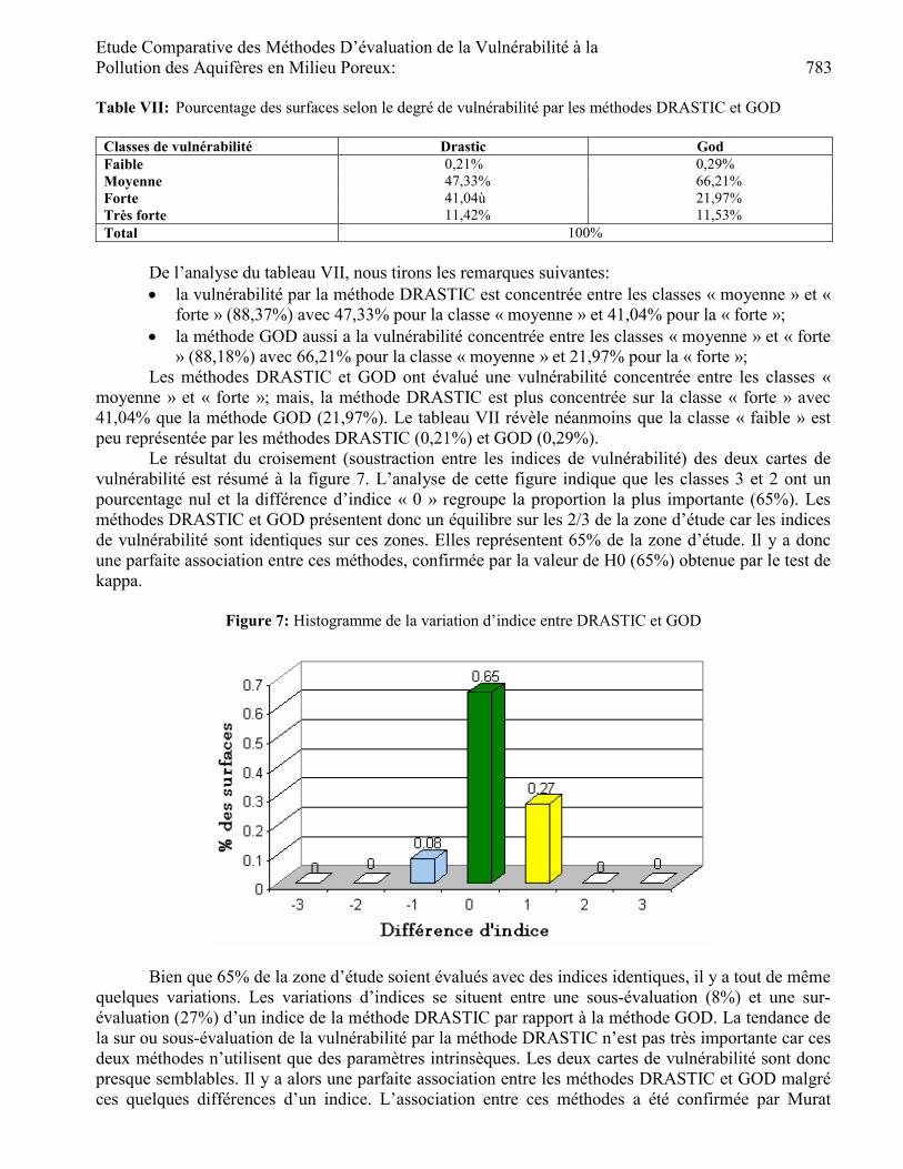
Etude Comparative des Méthodes D’évaluation de la Vulnérabilité à la Pollution des Aquifères en Milieu Poreux: 783
Table VII: Pourcentage des surfaces selon le degré de vulnérabilité par les méthodes DRASTIC et GOD
Classes de vulnérabilité Drastic God Faible 0,21% 0,29% Moyenne 47,33% 66,21% Forte 41,04ù 21,97% Très forte 11,42% 11,53% Total 100%
De l’analyse du tableau VII, nous tirons les remarques suivantes: • la vulnérabilité par la méthode DRASTIC est concentrée entre les classes « moyenne » et «
forte » (88,37%) avec 47,33% pour la classe « moyenne » et 41,04% pour la « forte »; • la méthode GOD aussi a la vulnérabilité concentrée entre les classes « moyenne » et « forte
» (88,18%) avec 66,21% pour la classe « moyenne » et 21,97% pour la « forte »; Les méthodes DRASTIC et GOD ont évalué une vulnérabilité concentrée entre les classes «
moyenne » et « forte »; mais, la méthode DRASTIC est plus concentrée sur la classe « forte » avec 41,04% que la méthode GOD (21,97%). Le tableau VII révèle néanmoins que la classe « faible » est peu représentée par les méthodes DRASTIC (0,21%) et GOD (0,29%).
Le résultat du croisement (soustraction entre les indices de vulnérabilité) des deux cartes de vulnérabilité est résumé à la figure 7. L’analyse de cette figure indique que les classes 3 et 2 ont un pourcentage nul et la différence d’indice « 0 » regroupe la proportion la plus importante (65%). Les méthodes DRASTIC et GOD présentent donc un équilibre sur les 2/3 de la zone d’étude car les indices de vulnérabilité sont identiques sur ces zones. Elles représentent 65% de la zone d’étude. Il y a donc une parfaite association entre ces méthodes, confirmée par la valeur de H0 (65%) obtenue par le test de kappa.
Figure 7: Histogramme de la variation d’indice entre DRASTIC et GOD
Bien que 65% de la zone d’étude soient évalués avec des indices identiques, il y a tout de même quelques variations. Les variations d’indices se situent entre une sous-évaluation (8%) et une sur-évaluation (27%) d’un indice de la méthode DRASTIC par rapport à la méthode GOD. La tendance de la sur ou sous-évaluation de la vulnérabilité par la méthode DRASTIC n’est pas très importante car ces deux méthodes n’utilisent que des paramètres intrinsèques. Les deux cartes de vulnérabilité sont donc presque semblables. Il y a alors une parfaite association entre les méthodes DRASTIC et GOD malgré ces quelques différences d’un indice. L’association entre ces méthodes a été confirmée par Murat

784 Kouamé kan Jean, Jourda Jean Patrice, Adja Miessan Germain, Deh Serges Kouakou, Anani Abenan Tawa, Effini Adiow Thérèse and Biémi Jean
(2000), Kimmeier (2001), Fofana (2005) et Anani (2006). Au regard des résultats de l’étude comparative, nous retenons que la méthode DRASTIC est la mieux indiquée dans la cartographie de la vulnérabilité à la pollution des eaux souterraines du District d’Abidjan. 5. Conclusion L’application des méthodes DRASTIC et GOD a permis d’évaluer la vulnérabilité intrinsèque à la pollution des eaux souterraines du District d’Abidjan. L’analyse des différentes cartes de vulnérabilité à la pollution a montré que la vulnérabilité par les méthodes DRASTIC et GOD est concentrée entre les classes moyenne et forte. La comparaison des cartes de vulnérabilité à partir du test de Kappa a montré qu’il existe un accord modéré entre ces méthodes (le coefficient Kappa vaut 0,418). L’analyse des fréquences de surface des cartes de vulnérabilité a révélé que les méthodes (DRASTIC et GOD) ont un parfait accord (65%), mais la méthode GOD a tendance à sur-évaluer la vulnérabilité d’un indice par rapport à DRASTIC.
La carte de vulnérabilité établie par les deux méthodes a été validée avec la carte de répartition spatiale du taux de nitrates de 2001. En effet, les deux méthodes utilisées ont montré qu’on assiste à une progression de la vulnérabilité du Sud vers le Nord. Les zones à fort taux de nitrates (> 50 mg/L) progressant également dans le même sens se superposent parfaitement aux zones de très forte à forte vulnérabilité. La superposition de ces deux types de zones (vulnérabilité forte et taux de nitrates élevé) permet de dire que la carte établie par ces méthodes reflète la réalité du terrain. Mais la carte de vulnérabilité réalisée à partir de la méthode DRASTIC reflète le mieux la réalité de la pollution des eaux souterraines du District d’Abidjan
Etude Comparative des Méthodes D’évaluation de la Vulnérabilité à la Pollution des Aquifères en Milieu Poreux: 785
References [1] Aghui N. et Biémi J. (1984). Géologie et hydrogéologie des nappes de la région d’Abidjan et
risques de contamination. Annales de l’Université Nationale de Côte d’Ivoire, série c tome 20, pp.331-347.
[2] Aller L., Bennett T., Lehr J.H., Petty R. J. et Hackett G. (1987). DRASTIC: A standardised system for evaluating ground water pollution potential using hydrogeologic settings. EPA, Ada, Oklahoma, 622 p.
[3] Anani A. T. épse Kouakou (2006). Evaluation et cartographie des zones vulnérables à la pollution des eaux souterraines au niveau du District d’Abidjan (Sud de la Côte d’Ivoire) par les méthodes DRASTIC et GOD. Mémoire de DEA, Université de Cocody, 71 p.
[4] Banton O. et Bangoy L. (1997). Hydrogéologie: Multiscience environnementale des eaux souterraines. Presse de l’Université du Québec, AUPELF, pp. 375 – 389
[5] Bézelgues S., Des Garets E., Mardhel V. et Dörfliger N. (2002). Cartographie de la vulnérabilité de Grand-Terre et de Marie-Galatie (Guadeloupe). Phase 1: méthodologie de détermination de la vulnérabilité, 45 p.
[6] Champagne L. et Chapuis R. P. (1993). Évaluation de la vulnérabilité à la pollution des formations aquifères de la MRC de Montcalm selon la méthode Drastic. Rev. Sc. Tech. Eau; 26; pp. 76 -169.
[7] Cohen J. (1970). A coefficient of agreement for nominal scales, Educ. Psychol. Meas, pp. 27-46.
[8] Douagui A. (2004). Evaluation de la vulnérabilité à la pollution de la nappe du Quaternaire du secteur "Canal de Vridi" – Grand-Bassam par la méthode DRASTIC. Mémoire de DEA, Université d’Abobo-Adjamé, 71 p.
[9] Fofana F. (2005). Evaluation et cartographie de la vulnérabilité à la pollution de la nappe d’Abidjan selon les méthodes DRASTIC et GOD. Mémoire de DEA, Université d’Abobo-Adjamé, 68 p.
[10] Foster S.S.D. (1987). Fundamental concepts in aquifer vulnerability, pollution risk and protection strategy. Atti Int. Conf. Vulnerability of soil and Groundwater to Pollutants, RIVM Proc. and Inf. 38. pp. 69-86.
[11] INS (2001). Recensement Général de la Population et de l’Habitation (RGPH) 1998. Données socio-démographiques et économiques des localités, résultats définitifs par localités, région des lagunes, vol.III, tome 1, 43 p.
[12] Isabel D., Gelinas P. et Aubre F. (1990). Cartographie de la vulnérabilité des eaux souterraines au Québec. Rev. Sc. Tech. Eau, 23 p.
[13] Jourda J. P. (2005). Méthodologie d’application des techniques de Télédétection et des systèmes d’information géographique à l’étude des aquifères fissurés d’Afrique de l’Ouest. Concept de l’hydrotechniquespatiale: cas des zones tests de la Côte d’Ivoire. Thèse de Doctorat d’Etat, Université de Cocody, 430 p.
[14] Jourda J. P., Kouamé K. F., Soro N., Kouamé K. J., Kouadio B. H., Saley M. B., Kouamé K et Ahoussi E. (2003). Gestion et protection des eaux souterraines urbaines: apports d’un système d’information géographique à la réalisation de la carte de vulnérabilité de la nappe du continental terminal au niveau de l’agglomération d’Abidjan. Dans les Actes de la conférence francophone SIG 2003, Paris, octobre 2003, 18 p.
[15] Jourda J. P., Saley M. B., Kouamé K. J., Kouadio B. H, Biémi J. et Razack M. (2005). Gestion et protection des ressources en eaux souterraines: contribution d’un SIG à la réalisation de la carte de vulnérabilité à la pollution des aquifères fissurés de Korhogo (nord de la Côte d’Ivoire) selon la méthode DRASTIC. Dans les Actes de la Conférence francophone SIG 2005, du 5 au 6 octobre 2005, Paris, 16 p.
[16] Jourda J. P.; Kouamé K. J., Saley M. B., Kouadio B.H. et Oga Y.S. (2006a): Contamination of the Abidjan aquifer by sewage: An assessment of extent and strategies for protection. In:
786 Kouamé kan Jean, Jourda Jean Patrice, Adja Miessan Germain, Deh Serges Kouakou, Anani Abenan Tawa, Effini Adiow Thérèse and Biémi Jean
Groundwater pollution in Africa (Edited by Yongxin X. and Brent U.), pp. 293-302, Taylor & Francis/Balkema, Great-Britain
[17] Jourda J. P., Kouamé K. J.; Saley M. B., Kouamé K. F., Kouadio B. H. et Kouamé K. (2006b). A new cartographic approach to determine the groundwater vulnerability of the Abidjan aquifer. In: Groundwater pollution in Africa (Edited by Yongxin X. and Brent U.), pp. 103-114, Taylor & Francis/Balkema, Great-Britain
[18] Kimmeier F. (2001). 3-D Groundwater flow modelling in heterogeneous geologic media: Integrated approach using spatial and temporal database, geostatistics and GIS. Thesis presented to the faculty of sciences of the Neuchâtel University, 223 p.
[19] Kouadio L., Abdoulaye S., Jourda P., Loba M. et Rambaud A. (1998). Conséquences de la pollution urbaine sur la distribution d’eau d’alimentation publique à Abidjan. Dans: Cahiers de l’Association Scientifique Européenne pour l’Eau et la Santé, vol.3, n°1, pp. 61 – 75.
[20] Kouamé K. J. (2003). Apports d’un système d’information géographique à la réalisation de la carte de vulnérabilité de la nappe du Continental terminal au niveau de l’agglomération d’Abidjan. Mémoire de DEA des Sciences de la Terre option hydrogéologie, Université de Cocody, 63 p.
[21] Kouamé K. J. (2007). Contribution à la Gestion Intégrée des Ressources en Eaux (GIRE) du District d’Abidjan (Sud de la Côte d’Ivoire): Outils d’aide à la décision pour la prévention et la protection des eaux souterraines contre la pollution. Thèse de Doctorat de l’Université de Cocody, 226 p.
[22] Landis J. R. et Koch G. G. (1977). The measurement of observer for categorical data, Biometrics, pp. 159-179.
[23] Lobo-Ferreira J. P., Novo E. M. et Oliveira M. M. (1995). Groundwater vulnerability mapping: Application to the Minho watershed in Northern Portugal’s Celtic Region. Laboratorio Nacional de Engenharia Civil, Lisbon, Portugal, 7 p.
[24] Lynch S. D., Reynders A. G. et Schulz R. (1993). Preparing input data for a national-scale groundwater vulnerability map of Southern Africa in 6th National Hydrological Symposium, SANCIAHS, September 1993 and water S.A. (1994) 20, pp. 239 – 246.
[25] Ministère du Plan et du Développement (MPD) (2006). Rapport national de l’Etat et le devenir de la population de la Côte d’Ivoire (REPCI). Population et développement: défis et perspectives pour la Côte d’Ivoire. UNFPA, août 2006.
[26] Mohamed R. M. (2001). Evaluation et cartographie de la vulnérabilité à la pollution de l’aquifère alluvionnaire de la plaine d’El Madher, Nord-Est algérien, selon la méthode DRASTIC. Sciences et changement planétaires / sécheresse, vol. 12, n°2, pp. 95-101.
[27] Murat V. (2000). Etude comparative des méthodes d’évaluation de la vulnérabilité intrinsèque des aquifères à la pollution: Application aux aquifères granulaires du Piémont LAURENTIEN. Mémoire de maîtrise, INRS – Géosciences, Québec, 127 p.
[28] Murat V., Martel R., Michaud Y. et Therrien R. (2000). Etude comparative des méthodes d’évaluation de la vulnérabilité des aquifères à la pollution: Application aux aquifères granulaires du Piémont LAURENTIEN, Québec, AIH-CNC et SCG, pp. 411-418.
[29] Murat V., Paradis D., Savard M. M., Nastev M., Bourque E., Hamel A., Lefebvre R. et Martel R. (2003). Vulnérabilité à la nappe des aquifères fracturés du sud-ouest du Québec: Evaluation par les méthodes DRASTIC et GOD. Ressources naturelles Canada, Commission Géologique, 16 p.
[30] Navalur k. C. S. et Engel B. A. (1997). Predicting spatial distribution of vulnerability of Indiana State Aquifer system to nitrate leaching using a GIS. 18 p.
[31] Tastet J. P. (1979). Environnements sédimentaires et structuraux quaternaires du littoral du Golfe de guinée (Côte d’Ivoire, Togo, Bénin). Thèse de Doctorat d’Etat ès sciences, Université de Bordeaux 1, 181 p.

Etude Comparative des Méthodes D’évaluation de la Vulnérabilité à la Pollution des Aquifères en Milieu Poreux: 787
[32] Vrba J. et Zaporozec A. (1994). Guidebook on mapping groundwater vulnerability. International association of hydrgeologists, vol.16, 131 p.
European Journal of Scientific Research ISSN 1450-216X Vol.20 No.4 (2008), pp.788-795 © EuroJournals Publishing, Inc. 2008 http://www.eurojournals.com/ejsr.htm
Development of an Interated Poultry/Fishery Husbandry for
Optimal Agricultural Production
F.R. Falayi Agricultural Engineering Department, The Federal University of Technology
P.M.B. 704, Akure, Ondo State, Nigeria
A.S. Ogunlowo Agricultural Engineering Department, The Federal University of Technology
P.M.B. 704, Akure, Ondo State, Nigeria
M.O. Alatise Agricultural Engineering Department, The Federal University of Technology
P.M.B. 704, Akure, Ondo State, Nigeria
Abstract
The need to find alternative but productive means of managing animal waste in the modern day agriculture waste cannot be over emphasised. One important means of managing these wastes is through conversion to important use either as animal feeds or as manures.
An integrated poultry/fishery housing unit was designed and constructed such that poultry droppings were made to drop into the ponds directly and used as feed for clarias gariepinus. The set-up was made of four concrete ponds on which three wooden battery cages were mounted except the fourth pond which served as the control. The ponds were stocked with twenty (20) juvenile clarias garipinus each. Fish in pond 1, two and three were fed with droppings from one broiler, two broilers and three broilers respectively. While fish in ponds 4 were fed with the fish concentrate. A total of 6 birds (4 weeks old) and 80 juvenile clarias gariepinus were used. This experiment lasted for 6 months. During this period of study, the environmental parameters were monitored and the effect of poultry waste on the development of the fish was analysed.
There was an increase in weight of the fish in all ponds through out the period of the study. The weight gained by the fish in pond 1 increased at an increasing rate of 10.85 g/week up to the 15th week after stocking. Thereafter, the weight gained started increasing at a constant rate of 86.8g/week up to the 20th week after stocking and thereafter a weight increase at a deceasing rate of 136.56 g/week up to harvest period. In pond 2, the weight of the fish increased at an increasing rate of 7.47 g/week up to 8th week. Thereafter, the weight gain increased at a constant rate of 24.88 g/week to 16th week and increasing at a decreasing rate of 42.75 g/week to harvest. The same trend was observed in pond 3 but the weight gain increased at an increasing rate of 8.06 g/week up to the 4th week and then increasing at a constant rate of 10.89 g/week to the 16th week. Thereafter, there was weight increase at a decreasing rate of 32.36 g/week to harvest. Pond 4, which was the control, showed a different trend in the development of the fish, in this case, there was a weight gain at an increasing rate of 12.90 g up to the 18th week after stocking. Thereafter there was a weight gain at a decreasing rate of 147.22 g/week up to harvest period.

Development of an Interated Poultry/Fishery Husbandry for Optimal Agricultural Production 789
Keywords: Integrated, fishery, poultry, droppings, pond
Introduction In many parts of the world, fish have provided an important part of people’s diet for centuries. The increasing per capita consumption of fish is partially due to consumer demand for healthy diet and the growing recognition that the fatty acid content of fish provides health benefit to man. The growth rate of the world’s human population has called for increased harvest of fish and fisheries products from marine and inland waters (Woynarovich 1979). Chandrasoma (1988) observed that during the last hundred years, fish catches have increased rapidly due to improved technologies. Despite the fact that growth in fish catches stopped some 15 years ago, over fishing had already caused the worldwide decrease in stock to become a real problem. The need to increase fish production by fish farming is urgent. Fish farming is an agricultural activity that can deeply improve the already existing farming system. As in agriculture, fish farming techniques include the removal of unwanted plants and animals, their replacement by desirable species, the improvement of these species by crossbreeding and selection, and the improvement of food availability by the use of fertilizer. Fish farming can benefit from agricultural by-products generated by other activities, as these activities can be used to increase the quality of plankton, that is, the natural food of fish (Chakrabarty and Hettiarachchi 1982). Fish farming can be combined with poultry, animal husbandry and irrigation practices, which can lead to higher production and net profits. This practice is called integrated fish farming or integrated aquaculture. The integration of animal husbandry, especially poultry, with fish farming in a small scale results in the production of organic manure for the fertilization of the fish pond to increase the production of the natural food organism (planktonic algae) to be eaten by the fish. In some cases, the poultry wastes are used as direct food by some fish without supplementary feedings, such species include Nile Tilapia (FAO, 1996).
There are various methods of integrating poultry with fish farming. Some designs give room for the poultry house to be sited on a land near the pond and the poultry waste/ manure is transferred into the pond manually. While another design sites the poultry directly on the pond. Literature regarding poultry/fish integration generally relates to battery or deep litter in which the birds are typically fed on complete diets in pelleted or mash form and the manure used as feed (Little and Muir, 1987). Manure is packed into the pond to fertilize it for the fish to feed. Not all fish are carnivores; therefore, not all can feed on manure. The herbivores rather pick waste supplemental feeds from the birds’ meal only. Integrated fish farming is regarded by aquaculturists of most countries as a model farming system for full utilization of local resources, for waste recycling and energy saving, and for maintaining ecological balance and circulation. Besides increasing the supply of fish, meat and eggs, and employment opportunities, it also reduces the cost of fish production through utilization of local farm products as fish feeds and fertilizers and reorganization of farm labour for effective output (De Silva 1991).
Although this technology is highly productive in certain regions in China and parts of Asia, Sharma 1981, reported that it is now recognized that large-scale technology transfer to most other regions, both inside and outside China, is dependent on a clearer scientific understanding of the physical, chemical and biological processes involved.
In developing countries like Nigeria, many are not informed about integrated fish farming and its attendant benefits. There is virtually no reliable data concerning the feasibility and adoption of the system. Adesulu (2001) stated that integrated fish farming is not a common practise in Nigeria. Thus this study was carried out in order to intensify our efforts on integrated agricultural production. 2. Methodology Model poultry housing unit and concrete fishponds were designed and constructed using locally available materials. Three wooden battery cages were mounted on the fish ponds. The set-up was made
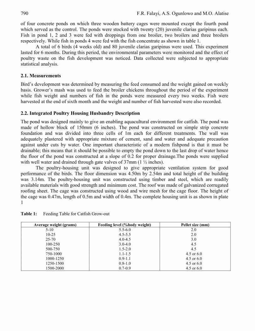
790 F.R. Falayi, A.S. Ogunlowo and M.O. Alatise
of four concrete ponds on which three wooden battery cages were mounted except the fourth pond which served as the control. The ponds were stocked with twenty (20) juvenile clarias garipinus each. Fish in pond 1, 2 and 3 were fed with droppings from one broiler, two broilers and three broilers respectively. While fish in ponds 4 were fed with the fish concentrate as shown in table 1.
A total of 6 birds (4 weeks old) and 80 juvenile clarias garipinus were used. This experiment lasted for 6 months. During this period, the environmental parameters were monitored and the effect of poultry waste on the fish development was noticed. Data collected were subjected to appropriate statistical analysis. 2.1. Measurements
Bird’s development was determined by measuring the feed consumed and the weight gained on weekly basis. Grower’s mash was used to feed the broiler chickens throughout the period of the experiment while fish weight and numbers of fish in the ponds were measured every two weeks. Fish were harvested at the end of sixth month and the weight and number of fish harvested were also recorded. 2.2. Integrated Poultry Housing Husbandry Description
The pond was designed mainly to give an enabling aquacultural environment for catfish. The pond was made of hollow block of 150mm (6 inches). The pond was constructed on simple strip concrete foundation and was divided into three cells of 1m each for different treatments. The wall was adequately plastered with appropriate mixture of cement, sand and water and adequate precaution against under cuts by water. One important characteristic of a modern fishpond is that it must be drainable; this means that it should be possible to empty the pond down to the last drop of water hence the floor of the pond was constructed at a slope of 0.2 for proper drainage.The ponds were supplied with well water and drained through gate valves of 37mm (1 ½ inches).
The poultry-housing unit was designed to give appropriate ventilation system for good performance of the birds. The floor dimension was 4.50m by 2.54m and total height of the building was 3.14m. The poultry-housing unit was constructed using timber and steel, which are readily available materials with good strength and minimum cost. The roof was made of galvanized corrugated roofing sheet. The cage was constructed using wood and wire mesh for the cage floor. The height of the cage was 0.47m, length of 0.5m and width of 0.4m. The complete housing unit is as shown in plate 1 Table 1: Feeding Table for Catfish Grow-out
Average weight (grams) Feeding level (%body weight) Pellet size (mm) 5-10 5.5-6.0 2.0 10-25 4.5-5.5 2.0 25-70 4.0-4.5 3.0 100-250 3.0-4.0 4.5 500-750 1.5-2.0 4.5 750-1000 1.1-1.5 4.5 or 6.0 1000-1250 0.9-1.1 4.5 or 6.0 1250-1500 0.8-1.0 4.5 or 6.0 1500-2000 0.7-0.9 4.5 or 6.0
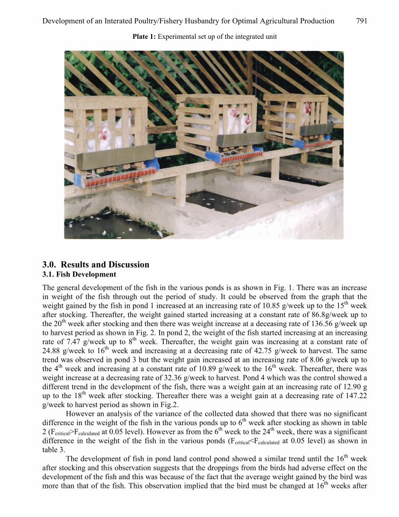
Development of an Interated Poultry/Fishery Husbandry for Optimal Agricultural Production 791
Plate 1: Experimental set up of the integrated unit
3.0. Results and Discussion 3.1. Fish Development
The general development of the fish in the various ponds is as shown in Fig. 1. There was an increase in weight of the fish through out the period of study. It could be observed from the graph that the weight gained by the fish in pond 1 increased at an increasing rate of 10.85 g/week up to the 15th week after stocking. Thereafter, the weight gained started increasing at a constant rate of 86.8g/week up to the 20th week after stocking and then there was weight increase at a deceasing rate of 136.56 g/week up to harvest period as shown in Fig. 2. In pond 2, the weight of the fish started increasing at an increasing rate of 7.47 g/week up to 8th week. Thereafter, the weight gain was increasing at a constant rate of 24.88 g/week to 16th week and increasing at a decreasing rate of 42.75 g/week to harvest. The same trend was observed in pond 3 but the weight gain increased at an increasing rate of 8.06 g/week up to the 4th week and increasing at a constant rate of 10.89 g/week to the 16th week. Thereafter, there was weight increase at a decreasing rate of 32.36 g/week to harvest. Pond 4 which was the control showed a different trend in the development of the fish, there was a weight gain at an increasing rate of 12.90 g up to the 18th week after stocking. Thereafter there was a weight gain at a decreasing rate of 147.22 g/week to harvest period as shown in Fig.2.
However an analysis of the variance of the collected data showed that there was no significant difference in the weight of the fish in the various ponds up to 6th week after stocking as shown in table 2 (Fcritical>Fcalculated at 0.05 level). However as from the 6th week to the 24th week, there was a significant difference in the weight of the fish in the various ponds (Fcritical<Fcalculated at 0.05 level) as shown in table 3.
The development of fish in pond land control pond showed a similar trend until the 16th week after stocking and this observation suggests that the droppings from the birds had adverse effect on the development of the fish and this was because of the fact that the average weight gained by the bird was more than that of the fish. This observation implied that the bird must be changed at 16th weeks after
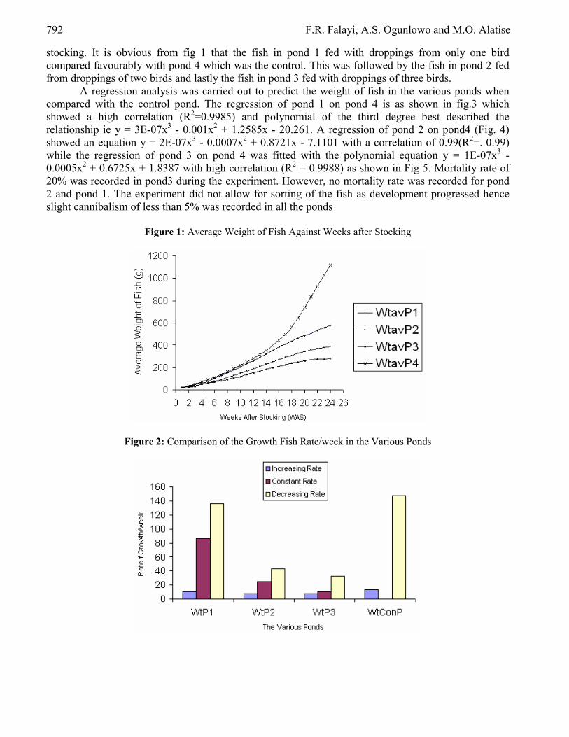
792 F.R. Falayi, A.S. Ogunlowo and M.O. Alatise
stocking. It is obvious from fig 1 that the fish in pond 1 fed with droppings from only one bird compared favourably with pond 4 which was the control. This was followed by the fish in pond 2 fed from droppings of two birds and lastly the fish in pond 3 fed with droppings of three birds.
A regression analysis was carried out to predict the weight of fish in the various ponds when compared with the control pond. The regression of pond 1 on pond 4 is as shown in fig.3 which showed a high correlation (R2=0.9985) and polynomial of the third degree best described the relationship ie y = 3E-07x3 - 0.001x2 + 1.2585x - 20.261. A regression of pond 2 on pond4 (Fig. 4) showed an equation y = 2E-07x3 - 0.0007x2 + 0.8721x - 7.1101 with a correlation of 0.99(R2=. 0.99) while the regression of pond 3 on pond 4 was fitted with the polynomial equation y = 1E-07x3 - 0.0005x2 + 0.6725x + 1.8387 with high correlation (R2 = 0.9988) as shown in Fig 5. Mortality rate of 20% was recorded in pond3 during the experiment. However, no mortality rate was recorded for pond 2 and pond 1. The experiment did not allow for sorting of the fish as development progressed hence slight cannibalism of less than 5% was recorded in all the ponds
Figure 1: Average Weight of Fish Against Weeks after Stocking
Figure 2: Comparison of the Growth Fish Rate/week in the Various Ponds
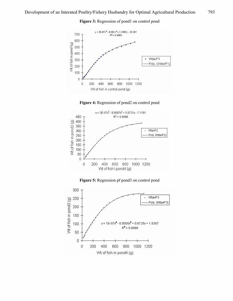
Development of an Interated Poultry/Fishery Husbandry for Optimal Agricultural Production 793
Figure 3: Regression of pond1 on control pond
Figure 4: Regression of pond2 on control pond
Figure 5: Regression pf pond3 on control pond
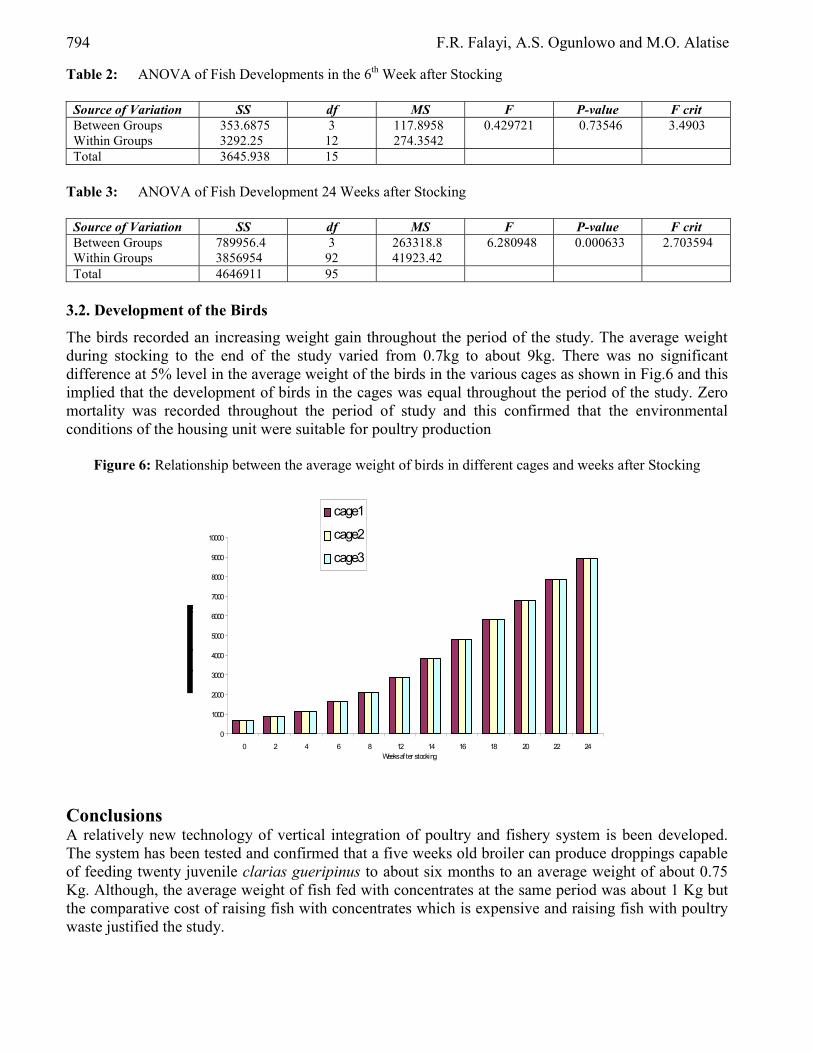
794 F.R. Falayi, A.S. Ogunlowo and M.O. Alatise
Table 2: ANOVA of Fish Developments in the 6th Week after Stocking
Source of Variation SS df MS F P-value F crit Between Groups 353.6875 3 117.8958 0.429721 0.73546 3.4903 Within Groups 3292.25 12 274.3542 Total 3645.938 15
Table 3: ANOVA of Fish Development 24 Weeks after Stocking
Source of Variation SS df MS F P-value F crit Between Groups 789956.4 3 263318.8 6.280948 0.000633 2.703594 Within Groups 3856954 92 41923.42 Total 4646911 95
3.2. Development of the Birds
The birds recorded an increasing weight gain throughout the period of the study. The average weight during stocking to the end of the study varied from 0.7kg to about 9kg. There was no significant difference at 5% level in the average weight of the birds in the various cages as shown in Fig.6 and this implied that the development of birds in the cages was equal throughout the period of the study. Zero mortality was recorded throughout the period of study and this confirmed that the environmental conditions of the housing unit were suitable for poultry production
Figure 6: Relationship between the average weight of birds in different cages and weeks after Stocking
0
1000
2000
3000
4000
5000
6000
7000
8000
9000
10000
0 2 4 6 8 12 14 16 18 20 22 24Weeks af ter stocking
cage1
cage2
cage3
Conclusions A relatively new technology of vertical integration of poultry and fishery system is been developed. The system has been tested and confirmed that a five weeks old broiler can produce droppings capable of feeding twenty juvenile clarias gueripinus to about six months to an average weight of about 0.75 Kg. Although, the average weight of fish fed with concentrates at the same period was about 1 Kg but the comparative cost of raising fish with concentrates which is expensive and raising fish with poultry waste justified the study.

Development of an Interated Poultry/Fishery Husbandry for Optimal Agricultural Production 795
References [1] Adesulu E.A. (2001). Pisciculture. External communication limited 1st edition, pp 65-67 [2] Chandrasoma J. (1988). Observations on Marketing of fish produced in seasonal tanks', Jour
Inland Fish Sri Lanka, 4: 63–67. [3] Chakrabarty R. D. & A. Hettiarachchi (1982). ‘Preliminary Observations on Fish Polyculture
cum Duck raising in a Farm Pond in Sri Lanka’, Jour Inland Fish. Sri Lanka, Vol 1. 54–61. [4] De Silva K. G. H. M. (1991). ‘The Predicament of the Freshwater Fisheries and Aquaculture of
Sri Lanka’, NAGA, The ICLARM Quarterly, Jan. 1991, pp. 6–7. [5] FAO (1996). Management for Freshwater Fish Culture. Ponds and water practices. FAO
Publication, 21/1, 233pp. [6] Ivor H. Seeley and Roger .W (1996). Building quantities explain: 5th Edition. Macmillan press
Limited, London. Page 87. [7] Little. D. and Muir, J. (1987). A guide to Integrated warm water aquaculture. published by the
Inst. Aquaculture, University of Stirring. Stirring Scotland. [8] Sharma B. K. (1981). Fish Culture Integrated with Livestock Raising; Summer Institute on
Farming System integrating agriculture, livestock and fish culture, 6 July - 4 August, Central Inland Fisheries Research Institute, Barackpore, West Bengal, pp. 128–142.
[9] Woynarovich E. (1979). The feasibility of combining animal husbandry with fish farming, with special reference to duck and pig production. In: Advanced in Aquaculture, T. V. R. Pillay and W. A. Dill (eds.). Fishing News Books Ltd. Farnham, Surrey, England, pp. 203–208.

European Journal of Scientific Research ISSN 1450-216X Vol.20 No.4 (2008), pp.796-804 © EuroJournals Publishing, Inc. 2008 http://www.eurojournals.com/ejsr.htm
Robust Control of a Doubly Fed Asynchronous Machine of a
Wind Turbine System
S. Gherbi
S. Yahmedi
M. Sedraoui
Abstract
In these last years, there is a growing interest to use the wind turbines systems to produce the electricity (see [1]) because it uses a renewable and non polluted energy which is the wind. There is different challenges in the control of the wind energy systems and we have to take in a count a several parameters that perturb the system as: the wind speed variation, the consumption variation of the electricity energy and the kind of the power consumed (active or reactive) ...etc. In this paper, we present a method to synthesize a robust controller for a wind turbine system based in a model equipped with doubly fed asynchronous machine which is the most used model in this last years [2] and we used the
∞H robust control method with the recent method based on the use of the linear matrix inequalities (LMI’s): Gahinet-Akparian [4], the results show the stability and the performance robustness of the system in spite of the perturbations mentioned before. Keywords: Doubly fed asynchronous machine, robust control, ∞H controller design
method, linear matrix inequality LMI I. Introduction From all the renewable energy electricity production systems, the wind turbine systems are the most used specially the doubly fed asynchronous machine based systems, the control of theses systems is particularly difficult because all of the uncertainties introduced such as: the wind speed variations, the electrical energy consumption variation, the system parameters variations, in this paper we focus on the robust control ( ∞H controller design method) of the doubly fed asynchronous machine which is the most used in the wind turbine system due to its low cost, simplicity of construction and maintenance [1]. This paper is organised as follow: section 2 presents the wind turbine systems equipped with the doubly fed asynchronous machine and the mathematical electrical equations are presented, then a model (in the state space form) are deducted, in the section 3 we present the ∞H robust controller design method used to control our system, the section 4 present a numerical application and the results in both the frequency and time plan are presented and conclusion is given in section 5. II. System Presentation and Modelling The wind turbines system is represented by the following figure:

Robust Control of a Doubly Fed Asynchronous Machine of a Wind Turbine System 797
Figure 1: Wind turbine system representation
The system use the wind power to drag the double fed asynchronous machine who acts as a generator, the output power produced must have the same high quality when it enters the electrical network, i.e: 220 volts amplitude and 60 Hz frequency and the harmonics held to a low level in spite of wind speed changes and electrical energy consumption in active or reactive power form. References [5], [6], [7] describe detailed models of wind turbines for simulations, we use the model equipped with the doubly fed induction generators (asynchronous machine) (for more details see [8]), the system electrical equations are given in ( )qd , frame orientation, then:
The stator voltage differential equations are:
qssdsdssds wdtdIRV Φ⋅−Φ+= . (1)
dssqsqssqs wdtdIRV Φ⋅+Φ+= . (2)
The rotor voltage differential equations are:
qrrdrdrrdr wdtdIRV Φ⋅−Φ+= . (3)
drrqrqrrqr wdtdIRV Φ⋅+Φ+= . (4)
The stator flux vectors equations are: drdssds IMIL .. +=Φ (5) qrqssqs IMIL .. +=Φ (6)
The rotor flux vectors equations: dsdrrdr IMIL .. +=Φ (7) qsqrrqr IMIL .. +=Φ (8)
The electromagnetic couple flux equation : )..(. drqsqrds
sem II
LMpC Φ−Φ= (9)
The electromagnetic couple mecanic equation: Ω+
Ω+= .f
dtdJCC rem (10)
Where: qsds VV , : Statoric voltage vector components in ‘d’ and ‘q’ axes respectively.
qrdr VV , : Rotoric voltage vector components in ‘d’ and ‘q’ axes respectively.
qsds II , : Statoric current vector components in ‘d’ and ‘q’ axes respectively.
qrdr II , : Rotoric current vector components in ‘d’ and ‘q’ axes respectively.
qsds ΦΦ , : Statoric flux vector components in ‘d’ and ‘q’ axes respectively.
qrdr ΦΦ , : Rotoric flux vector components in ‘d’ and ‘q’ axes respectively.

798 S. Gherbi, S. Yahmedi and M. Sedraoui
rs RR , : Stator and rotor resistances (of one phase) respectively. rs LL , : Stator and rotor cyclic inductances respectively. rs ww , : Statoric and rotoric current pulsations respectively.
M : Cyclic mutual inductance. p : Number of pair of the machine poles.
rC : Resistant torque. f : Viscous rubbing coefficient. J : Inertia moment.
2.1. State space Model
In order to apply the robust controller design method, we have to put the system model in the state space from; we consider the rotoric voltage qrdr V,V as the inputs and the statoric voltage qsds VV , as the outputs, i.e. we have to design a controller who acts on the rotoric voltages to keep the output statoric voltages at volts220 and Hz50 frequency in spite of the electric network perturbations (demand variations … etc) and the wind speed variations (see fig.2).
Figure 2: A Doubly fed wind turbine system control configuration
Where: u , y and e are the rotoric voltage vector (control vector), statoric output voltage vector and the error signal between the input reference and the output system respectively. K , G are the controller, wind turbine system respectively. R is the statoric voltage references vector and
onsperturbati are the electric energy demand variations, wind speed variations …etc. • Let us consider [ ]Tqrdrx ΦΦ= as a state vector, and [ ]Tqsdsqsds VVIIu = as the command
vector, the stator flux vector is oriented in d axis of Parks reference frame then : 0=Φ qs and
qsds II , are considered constant in the steady state ie: 0== qsds II && . • We use the folowing doubly fed asynchronous machine parameters:
Ω= 5sR ; Ω= 0113.1rR ; HM 1346.0= HLs 3409.0= ; HLr 605.0= ; Hzwr 6.146= ; Hzws 502 ⋅= π
Let rs www −= and rs LL
M⋅
−=2
1σ .
• The state space (11) can be obtained by the combining of the equations (1) to (8) as follow:
⎩⎨⎧
⋅+⋅=⋅+⋅=
uDxCyuBxAx& (11)
Where: [ ]Tqrdrx φφ= , [ ]Tqrdrqsds VVIIu = , [ ]Tqsds VVy = and :
⎥⎥⎥⎥
⎦
⎤
⎢⎢⎢⎢
⎣
⎡
−−
−
=
r
rr
rr
r
LR
w
wLR
A ,⎥⎥⎥⎥
⎦
⎤
⎢⎢⎢⎢
⎣
⎡
=10.0
010.
r
r
r
r
LMR
LMR
B

Robust Control of a Doubly Fed Asynchronous Machine of a Wind Turbine System 799
⎥⎥⎥⎥
⎦
⎤
⎢⎢⎢⎢
⎣
⎡
−⋅−=
r
r
r
r
rLRw
wLR
LMC ,
⎥⎥⎥⎥⎥
⎦
⎤
⎢⎢⎢⎢⎢
⎣
⎡
⋅+⋅
⋅−⋅+=
rr
rss
rsr
rs
LMR
LMRWL
LMWLR
LMR
D0.
0.
2
2
2
2
σ
σ
III. The H∞ Controller Design Method It is necessary to recall the basics of a control loop (fig.3), with: m∆ : is the system uncertainty, K: the controller , G: the nominal system.
Figure 3: The control loop with the output multiplicative uncertainties
The multiplicative uncertainties at the process output which include all the perturbations that act in the system are then : 1' ).( −−=∆ GGGm , with )( mIGG ∆+=′ : is the perturbed system, (Fig.3) show the singular values plot at the frequency plan of m∆ , we can see that the uncertainties are smaller at low frequencies and grow at the medium and high frequencies, this mean a strong perturbation at high frequencies (the transient phase), we also note a pick at the pulsation: sec/260rad=ω due to the fact that the system is highly coupled at this pulsation.
We can bound the system uncertainties by the following weighting matrix function:
⎥⎥⎥⎥
⎦
⎤
⎢⎢⎢⎢
⎣
⎡
++
++
=
)0001.01()102.0(55.00
0)0001.01()102.0(55.0
)(
jwjw
jwjw
jwWt (12)
The robust stability condition [11] is then: ( ) ( )[ ] 1pjwWjwT t⋅σ (13)
Or: ( )[ ] ( )[ ] 1−< jwWjwT tσσ (14) Where: ( )jwT is the nominal closed loop transfer matrix defined by: ( ) ( ) ( ) ( ) ( )[ ] 1−⋅+⋅⋅= jwKjwGIjwKjwGjwT (15)
The equations (13) allow us to guaranty the stability robustness, in other hand we most guaranty satisfying performances (no overshoot, satisfying time response …etc) in the closed loop (performances robustness), this can by done by the performance robustness condition [12]:
( ) ( )[ ] 1pjwWjwS p⋅σ (16)
Or: ( )[ ] ( )[ ] 1−< jwWjwS pσσ (17) Where:
• ( )jwS is the sensitivity matrix given by: ( ) ( ) ( )[ ] 1−⋅+= jwKjwGIjwS (18)
• )( jwWP is a weighting matrix function designed to meet the performance specifications desired in the frequency plan, we choose the following matrix function:
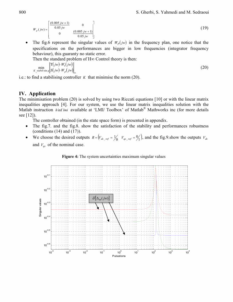
800 S. Gherbi, S. Yahmedi and M. Sedraoui
⎥⎥⎥⎥
⎦
⎤
⎢⎢⎢⎢
⎣
⎡
+
+
=
jwjw
jwjw
jwW p
05.0)1005.0(0
005.0
)1005.0(
)( (19)
• The fig.6 represent the singular values of ( )jwWP in the frequency plan, one notice that the specifications on the performances are bigger in low frequencies (integrator frequency behaviour), this guaranty no static error. Then the standard problem of H∞ Control theory is then:
( ) ( )( ) ( )
∞⋅⋅
jwWjwSjwWjw
pgstabiliK
t
sin
Tmin (20)
i.e.: to find a stabilising controller K that minimise the norm (20). IV. Application The minimisation problem (20) is solved by using two Riccati equations [10] or with the linear matrix inequalities approach [4]. For our system, we use the linear matrix inequalities solution with the Matlab instruction lmih inf available at ‘LMI/ Toolbox’ of Matlab® Mathworks inc (for more details see [12]).
The controller obtained (in the state space form) is presented in appendix. • The fig.7. and the fig.8. show the satisfaction of the stability and performances robustness
(conditions (14) and (17)). • We choose the desired outputs ( )1
00
1__ === refqsrefds VVR , and the fig.9.show the outputs dsV
and qsV of the nominal case.
Figure 4: The system uncertainties maximum singular values
10-4
10-3
10-2
10-1
100
101
102
103
104
10-0.6
10-0.5
10-0.4
10-0.3
10-0.2
10-0.1
Pulsations
Sin
gula
r va
lues
[ ])( jwm∆σ
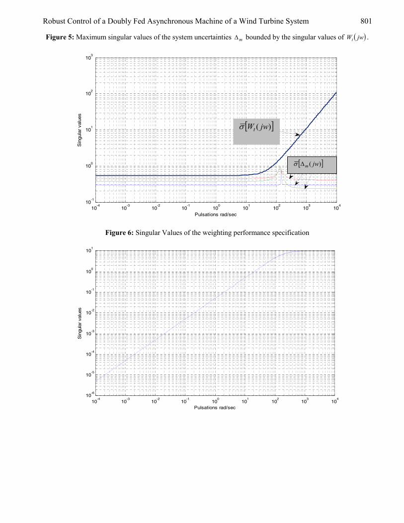
Robust Control of a Doubly Fed Asynchronous Machine of a Wind Turbine System 801
Figure 5: Maximum singular values of the system uncertainties m∆ bounded by the singular values of ( )jwWt .
10-4
10-3
10-2
10-1
100
101
102
103
104
10-1
100
101
102
103
Pulsations rad/sec
Sin
gula
r va
lues
[ ])( jwWtσ
[ ])( jwm∆σ
Figure 6: Singular Values of the weighting performance specification
10-4
10-3
10-2
10-1
100
101
102
103
104
10-6
10-5
10-4
10-3
10-2
10-1
100
101
Pulsations rad/sec
Sin
gula
r va
lues

802 S. Gherbi, S. Yahmedi and M. Sedraoui
Figure 7: Stability robustness condition
10-4
10-3
10-2
10-1
100
101
102
103
104
10-5
10-4
10-3
10-2
10-1
100
101
Pulsations rad/sec
Sin
gula
r va
lues
[ ])( jwTσ
[ ] 1)( −jwWtσ
Figure 8: Performances robustness condition
10-4
10-3
10-2
10-1
100
101
102
103
104
10-6
10-5
10-4
10-3
10-2
10-1
100
101
Pulsations rad/sec
Sin
gula
r va
lues
[ ])( jwSσ
[ ] 1)( −jwWpσ
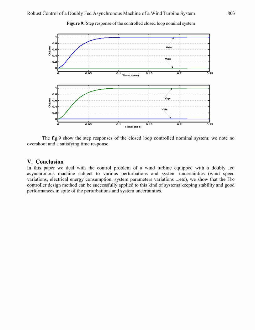
Robust Control of a Doubly Fed Asynchronous Machine of a Wind Turbine System 803
Figure 9: Step response of the controlled closed loop nominal system
0 0.05 0.1 0.15 0.2 0.25
0
0.2
0.4
0.6
0.8
1
Time (sec)
Outp
uts
0 0.05 0.1 0.15 0.2 0.25
0
0.2
0.4
0.6
0.8
1
Time (sec)
Outp
uts
Vds
Vqs
Vqs
Vds
The fig.9 show the step responses of the closed loop controlled nominal system; we note no overshoot and a satisfying time response. V. Conclusion In this paper we deal with the control problem of a wind turbine equipped with a doubly fed asynchronous machine subject to various perturbations and system uncertainties (wind speed variations, electrical energy consumption, system parameters variations ...etc), we show that the H∞ controller design method can be successfully applied to this kind of systems keeping stability and good performances in spite of the perturbations and system uncertainties.

804 S. Gherbi, S. Yahmedi and M. Sedraoui References [1] G. L. Johnson, ‘ Wind energy systems : Electronic Edition’, Manhattan, KS, October 10, 2006. [2] ‘AWEA Electrical Guide to Utility Scale Wind Turbines’, The American Wind Energy
Association, March 2005, available at http://www.awea.org. [3] J. C. Doyle, K. Glover, P. P. Khargonekar and Bruce A. Francis, ‘ State-Space Solution to
Standard H2 and H∞ Control Problems’, IEEE Transactions on Automatic Control, Vol. 34, N°. 8, August 1989.
[4] P. Gahinet, P. Akparian. ‘A linear Matrix Inequality Approch to H∞ Control ‘, Int. J. of Robust & Nonlinear Control“, vol. 4, pp. 421-448, 1994.
[5] J. Soens, J. Driesen, R. Belmans, ‘ Equivalent Transfer Function for a Variable-speed Wind Turbine in Power System Dynamic Simulations ‘, International Journal of Distributed Energy Resources, Vol.1 N°2, April-June, 2005; pp. 111-133.
[6] ‘Dynamic Modelling of Doubly-Fed Induction Machine Wind-Generators’, DigSilent GmbH Technical Documentation, 2003, available at http://www.digsilent.de.
[7] J. Soens, J. Driesen, R. Belmans, ‘ Wind turbine modelling approaches for dynamic power system simulations ‘, IEEE Young Researchers Symposium in Electrical Power Engineering - Intelligent Energy Conversion, (CD-Rom), Delft, The Netherlands, March 18-19, 2004.
[8] J. Soens, V. Van Thong, J. Driesen, R. Belmans , ‘ Modelling wind turbine generators for power system simulations ‘, European Wind Energy Conference EWEC, Madrid, 16 – 19 June 2003.
[9] Sigurd Skogestad, Ian Postlethwaite, ‘Multivariable Feedback Control Analysis and Design’, John Wiley and Sons, 1996. pp: 72 to 75
[10] J . C. Doyle, K. Glover, P. P. Khargonekar and Bruce A. Francis, ‘State-Space Solution to Standard 2H and ∞H Control Problems’, IEEE Transactions on Automatic Control, Vol. 34, N°. 8, August 1989.
[11] D.-W. Gu, P. Hr. Petkov and M. M. Konstantinov, ‘Robust Control Design with MATLAB®’, © Springer-Verlag London Limited 2005.pp:27 to 29
[12] P. Gahinet, A. Nemirovski, A. J. Laub, M. Chilali. “LMI Control Toolbox For Use with MATLAB® ”, User’s Guide Version 1, The MathWorks, Inc. 1995.
European Journal of Scientific Research ISSN 1450-216X Vol.20 No.4 (2008), pp.805-816 © EuroJournals Publishing, Inc. 2008 http://www.eurojournals.com/ejsr.htm
Effects of Enviromental Variables on
Poultry Performance and Pond Water Quality in an Integrated Poultry/Fishery Farming
F.R. Falayi Agricultural Engineering Department, The Federal University of Technology
P.M.B. 704, Akure, Ondo State, Nigeria
A.S. Ogunlowo Agricultural Engineering Department, The Federal University of Technology
P.M.B. 704, Akure, Ondo State, Nigeria
M.O. Alatise Agricultural Engineering Department, The Federal University of Technology
P.M.B. 704, Akure, Ondo State, Nigeria
Abstract
The need to find alternative but productive means of managing animal waste in the modern day agriculture waste cannot be over emphasised. One important means of managing these wastes is through conversion to important use either as animal feeds or as manures. Fish farming can be combined with poultry, animal husbandry and irrigation practices, which can lead to higher production and net profits. This practice is called integrated fish farming or integrated aquaculture. The integration of animal husbandry, especially poultry, with fish farming in a small scale results in the production of organic manure for the fertilization of the fish pond to increase the production of the natural food organism (planktonic algae) to be eaten by the fish. In some cases, the poultry wastes are used as direct food by some fish without supplementary feedings, such species include Nile Tilapia and catfish
An integrated poultry/fishery housing unit was designed and constructed such that poultry droppings were made to drop into the ponds directly and used as feed for clarias gariepinus. The set-up was made of four concrete ponds on which three wooden battery cages were mounted except the fourth pond which served as the control. The ponds were stocked with twenty (20) juvenile clarias garipinus each. There were four treatments and 3 replicates, fish in pond 1, two and three were fed with droppings from one broiler, two broilers and three broilers respectively. While fish in ponds 4 were fed with the fish concentrate. A total of 6 birds (4 weeks old) and 80 juvenile clarias gariepinus were used. This experiment lasted for 6 months. During this period, the environmental parameters were monitored and the effect of poultry waste on the development of the fish was analysed.
There were remarkable differences in the microclimate inside and outside the building. The birds were well protected from harsh environmental conditions and a uniform development was recorded. Pollution resulting from the use of poultry droppings adversely affected the development of the fish. Increase in the volume of droppings led to increase in the Bio-Chemical oxygen demand and Chemical Oxygen demand of the pond water which
Effects of Enviromental Variables on Poultry Performance and Pond Water Quality in an Integrated Poultry/Fishery Farming 806
consequently led to a decrease in the dissolved oxygen. Water turbidity also increased with increased droppings. Other water parameters like conductivity, chloride and pH values were within acceptable values suggested in literatures.
The system has shown the possibility of effective poultry waste management technique which ensured that nothing is wasted and waste handling problem is grossly reduced. Keywords: Integrated, fishery, poultry, droppings, pond
1. Introduction In many parts of the world, fish have provided an important part of people’s diet for centuries. The increasing per capita consumption of fish is partially due to consumer demand for healthy diet and the growing recognition that the fatty acid content of fish provides health benefit to man. The growth rate of the world’s human population has called for increased harvest of fish and fisheries products from marine and inland waters (Woynarovich 1979). Chandrasoma (1988) observed that during the last hundred years, fish catches have increased rapidly due to improved technologies. The need to increase fish production by fish farming is urgent. Fish farming is an agricultural activity that can deeply improve the already existing farming system. As in agriculture, fish farming techniques include the removal of unwanted plants and animals, their replacement by desirable species, the improvement of these species by crossbreeding and selection, and the improvement of food availability by the use of fertilizer. Fish farming can benefit from agricultural by-products generated by other activities, as these activities can be used to increase the quality of plankton, that is, the natural food of fish (Chakrabarty and Hettiarachchi 1982). Fish farming can be combined with poultry, animal husbandry and irrigation practices, which can lead to higher production and net profits. This practice is called integrated fish farming or integrated aquaculture. The integration of animal husbandry, especially poultry, with fish farming in a small scale results in the production of organic manure for the fertilization of the fish pond to increase the production of the natural food organism (planktonic algae) to be eaten by the fish. In some cases, the poultry wastes are used as direct food by some fish without supplementary feedings, such species include Nile Tilapia (FAO, 1996).
Intensive livestock housing such as livestock-fish farming employs an environmental control system to maintain animal health and welfare and raise production efficiency. The thermal environment within an animal house can be defined in terms of air temperature, relative humidity, thermal radiation and air velocity. Air temperature and sometimes relative humidity, are commonly used as the criteria by which the rate of ventilation is controlled (Charles 1994).
Adverse environments can affect the incidence and severity of certain endemic diseases. For example, a poor indoor microclimate, which is characterized by an inadequate thermal environment, poor ventilation and high burden of aerial pollutants, can play a major role in the aetiology of enzootic bronchopneumonia of calves and weaner pigs (Eikmeier and Mayer 1965).
Several authors have discussed and reported the effect of temperature on the milk yield of dairy cow, the performance of fattening pigs and the egg yield of laying hens. The lower critical temperature (LCT) defines the lower limit of the range of optimal temperature: the upper limit is given by the upper critical temperature (UCT). LCT is affected by factors such as age, sex, breed, food energy level and intake, feathering, stocking density, bedding system, etc. UCT values are rarely exceeded for housed livestock in temperate climates but a serious problem in the tropical humid climate like Nigeria. The CIGR commission recommended maximum and minimum values of relative humidity (RH) as a function of indoor temperature, for example an RH of 50-90% at 0ºC followed by a steady decrease of RH to a tolerable range of 40-60% at 30ºC.
807 F.R. Falayi, A.S. Ogunlowo and M.O. Alatise
The object of this study was to investigate the effect micro-climate parameters like temperature and relative humidity in an integrated husbandry with respect to physiological, growth and health aspects. The development of the fish and birds have been reported elsewhere. Materials and Methods Model poultry housing unit and concrete fishponds were designed and constructed using locally available materials. Three wooden battery cages were mounted on the fish ponds. The set-up was made of four concrete ponds on which three wooden battery cages were mounted except the fourth pond which served as the control. The ponds were stocked with twenty (20) juvenile clarias garipinus each. Fish in pond 1, 2 and 3 were fed with droppings from one broiler, two broilers and three broilers respectively. While fish in ponds 4 were fed with the fish concentrate as shown in table 1. Table 1: Feeding Table for Catfish Grow-out
Average weight (grams) Feeding level (%body weight) Pellet size (mm) 5-10 5.5-6.0 2.0 10-25 4.5-5.5 2.0 25-70 4.0-4.5 3.0 100-250 3.0-4.0 4.5 500-750 1.5-2.0 4.5 750-1000 1.1-1.5 4.5 or 6.0 1000-1250 0.9-1.1 4.5 or 6.0 1250-1500 0.8-1.0 4.5 or 6.0 1500-2000 0.7-0.9 4.5 or 6.0
A total of 6 birds (4 weeks old) and 80 juvenile clarias garipinus were used. This experiment
lasted for 6 months. During this period, the environmental parameters were monitored and the effect of poultry waste on the fish development was observed.
Air temperature and humidity inside the husbandry were measured using a combined thermistor and capacitive sensor with a range of 5 to 60ºC and 0-100% RH, respectively. The accuracy at 25ºC was ± 0.5ºC and ± 2% RH. Data collected were stored using a data logger. The procedure is similar to Seedorf et al 1998. The relationship between external and internal temperatures was analysed.
Direct analysis was used to determine water temperature (0C), Turbidity (NTU), pH, Conductivity (µscm-1), Dissolved oxygen (mg/l) and Salinity (%) using Horiba U 10 portable water analyser, while chemical analysis was used to determine chemical components which include; Nitrite, Ammonia, colour, Biochemical oxygen demand (BOD), Chloride, Chemical oxygen demand (COD), Dissolved oxygen (DO). 3. Integrated Poultry Housing Husbandry Description The pond was designed mainly to give an enabling aquacultural environment for catfish. The pond was made of hollow block of 150mm (6 inches). The pond was constructed on simple strip concrete foundation and was divided into three cells of 1m each for different treatments. The wall was adequately plastered with appropriate mixture of cement, sand and water and adequate precaution against under cuts by water. One important characteristic of a modern fishpond is that it must be drainable; this means that it should be possible to empty the pond down to the last drop of water hence the floor of the pond was constructed at a slope of 0.2 for proper drainage. The ponds were supplied with well water and drained through gate valves of 37mm (1 ½ inches).
The poultry-housing unit was designed to give appropriate ventilation system for good performance of the birds. The floor dimension was 4.50m by 2.54m and total height of the building was 3.14m. The poultry-housing unit was constructed using timber and steel, which are readily
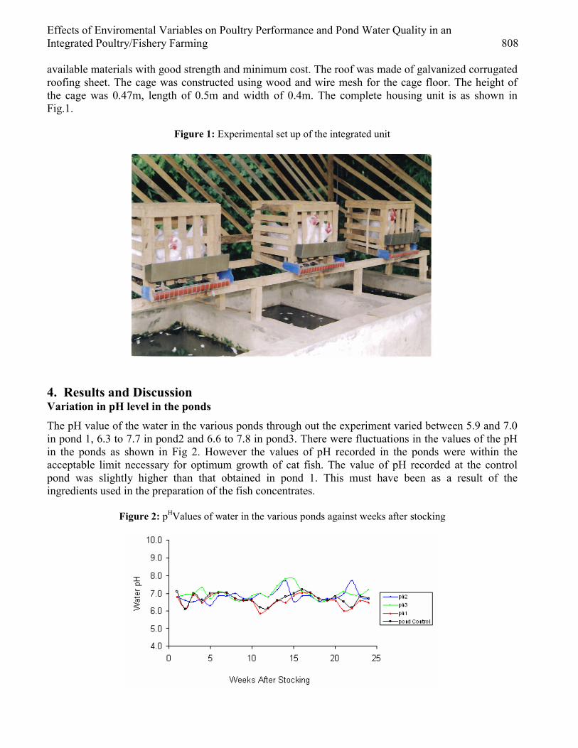
Effects of Enviromental Variables on Poultry Performance and Pond Water Quality in an Integrated Poultry/Fishery Farming 808 available materials with good strength and minimum cost. The roof was made of galvanized corrugated roofing sheet. The cage was constructed using wood and wire mesh for the cage floor. The height of the cage was 0.47m, length of 0.5m and width of 0.4m. The complete housing unit is as shown in Fig.1.
Figure 1: Experimental set up of the integrated unit
4. Results and Discussion Variation in pH level in the ponds
The pH value of the water in the various ponds through out the experiment varied between 5.9 and 7.0 in pond 1, 6.3 to 7.7 in pond2 and 6.6 to 7.8 in pond3. There were fluctuations in the values of the pH in the ponds as shown in Fig 2. However the values of pH recorded in the ponds were within the acceptable limit necessary for optimum growth of cat fish. The value of pH recorded at the control pond was slightly higher than that obtained in pond 1. This must have been as a result of the ingredients used in the preparation of the fish concentrates.
Figure 2: pHValues of water in the various ponds against weeks after stocking
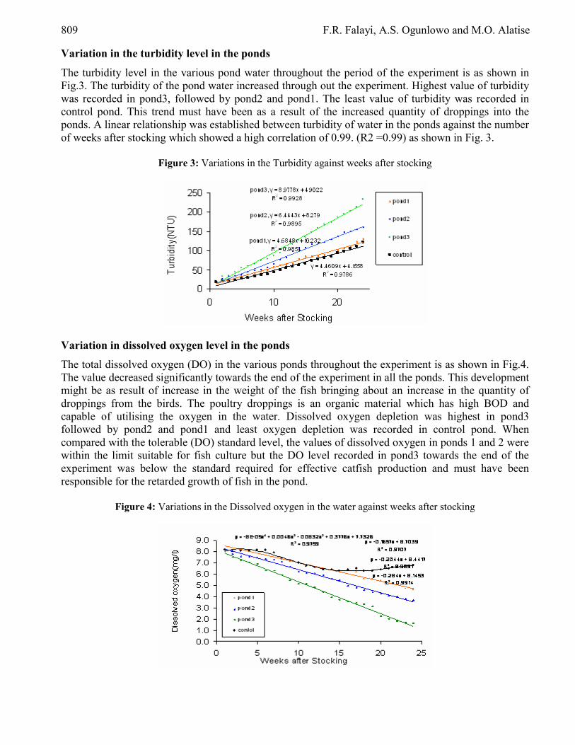
809 F.R. Falayi, A.S. Ogunlowo and M.O. Alatise
Variation in the turbidity level in the ponds
The turbidity level in the various pond water throughout the period of the experiment is as shown in Fig.3. The turbidity of the pond water increased through out the experiment. Highest value of turbidity was recorded in pond3, followed by pond2 and pond1. The least value of turbidity was recorded in control pond. This trend must have been as a result of the increased quantity of droppings into the ponds. A linear relationship was established between turbidity of water in the ponds against the number of weeks after stocking which showed a high correlation of 0.99. (R2 =0.99) as shown in Fig. 3.
Figure 3: Variations in the Turbidity against weeks after stocking
Variation in dissolved oxygen level in the ponds
The total dissolved oxygen (DO) in the various ponds throughout the experiment is as shown in Fig.4. The value decreased significantly towards the end of the experiment in all the ponds. This development might be as result of increase in the weight of the fish bringing about an increase in the quantity of droppings from the birds. The poultry droppings is an organic material which has high BOD and capable of utilising the oxygen in the water. Dissolved oxygen depletion was highest in pond3 followed by pond2 and pond1 and least oxygen depletion was recorded in control pond. When compared with the tolerable (DO) standard level, the values of dissolved oxygen in ponds 1 and 2 were within the limit suitable for fish culture but the DO level recorded in pond3 towards the end of the experiment was below the standard required for effective catfish production and must have been responsible for the retarded growth of fish in the pond.
Figure 4: Variations in the Dissolved oxygen in the water against weeks after stocking
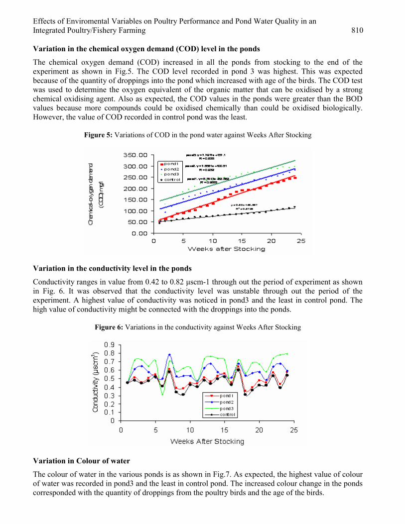
Effects of Enviromental Variables on Poultry Performance and Pond Water Quality in an Integrated Poultry/Fishery Farming 810 Variation in the chemical oxygen demand (COD) level in the ponds
The chemical oxygen demand (COD) increased in all the ponds from stocking to the end of the experiment as shown in Fig.5. The COD level recorded in pond 3 was highest. This was expected because of the quantity of droppings into the pond which increased with age of the birds. The COD test was used to determine the oxygen equivalent of the organic matter that can be oxidised by a strong chemical oxidising agent. Also as expected, the COD values in the ponds were greater than the BOD values because more compounds could be oxidised chemically than could be oxidised biologically. However, the value of COD recorded in control pond was the least.
Figure 5: Variations of COD in the pond water against Weeks After Stocking
Variation in the conductivity level in the ponds
Conductivity ranges in value from 0.42 to 0.82 µscm-1 through out the period of experiment as shown in Fig. 6. It was observed that the conductivity level was unstable through out the period of the experiment. A highest value of conductivity was noticed in pond3 and the least in control pond. The high value of conductivity might be connected with the droppings into the ponds.
Figure 6: Variations in the conductivity against Weeks After Stocking
Variation in Colour of water
The colour of water in the various ponds is as shown in Fig.7. As expected, the highest value of colour of water was recorded in pond3 and the least in control pond. The increased colour change in the ponds corresponded with the quantity of droppings from the poultry birds and the age of the birds.
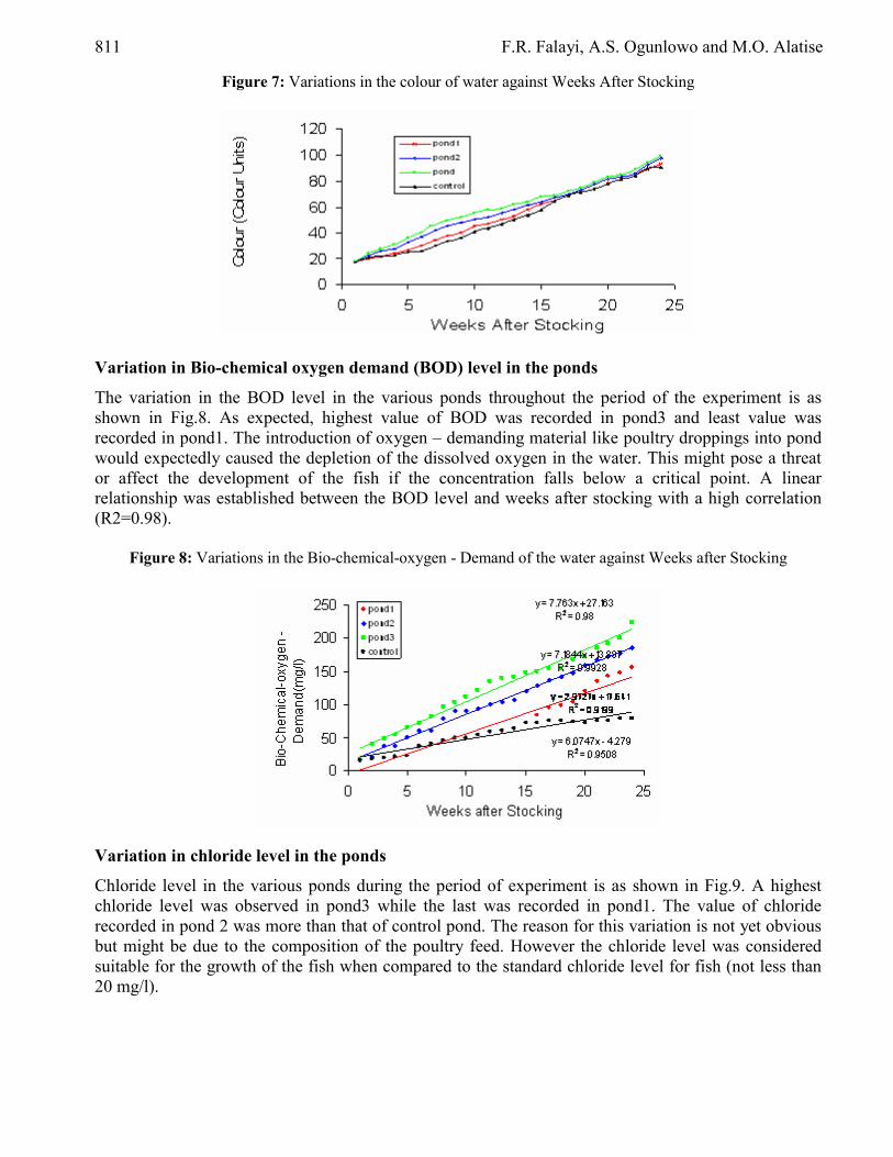
811 F.R. Falayi, A.S. Ogunlowo and M.O. Alatise
Figure 7: Variations in the colour of water against Weeks After Stocking
Variation in Bio-chemical oxygen demand (BOD) level in the ponds
The variation in the BOD level in the various ponds throughout the period of the experiment is as shown in Fig.8. As expected, highest value of BOD was recorded in pond3 and least value was recorded in pond1. The introduction of oxygen – demanding material like poultry droppings into pond would expectedly caused the depletion of the dissolved oxygen in the water. This might pose a threat or affect the development of the fish if the concentration falls below a critical point. A linear relationship was established between the BOD level and weeks after stocking with a high correlation (R2=0.98).
Figure 8: Variations in the Bio-chemical-oxygen - Demand of the water against Weeks after Stocking
Variation in chloride level in the ponds
Chloride level in the various ponds during the period of experiment is as shown in Fig.9. A highest chloride level was observed in pond3 while the last was recorded in pond1. The value of chloride recorded in pond 2 was more than that of control pond. The reason for this variation is not yet obvious but might be due to the composition of the poultry feed. However the chloride level was considered suitable for the growth of the fish when compared to the standard chloride level for fish (not less than 20 mg/l).
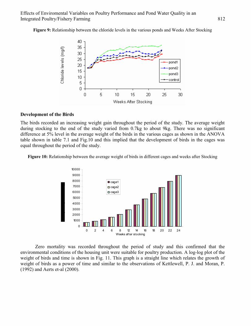
Effects of Enviromental Variables on Poultry Performance and Pond Water Quality in an Integrated Poultry/Fishery Farming 812
Figure 9: Relationship between the chloride levels in the various ponds and Weeks After Stocking
Development of the Birds
The birds recorded an increasing weight gain throughout the period of the study. The average weight during stocking to the end of the study varied from 0.7kg to about 9kg. There was no significant difference at 5% level in the average weight of the birds in the various cages as shown in the ANOVA table shown in table 7.1 and Fig.10 and this implied that the development of birds in the cages was equal throughout the period of the study.
Figure 10: Relationship between the average weight of birds in different cages and weeks after Stocking
0
1000
2000
3000
4000
5000
6000
7000
8000
9000
10000
0 2 4 6 8 12 14 16 18 20 22 24Weeks af ter stocking
cage1cage2cage3
Zero mortality was recorded throughout the period of study and this confirmed that the environmental conditions of the housing unit were suitable for poultry production. A log-log plot of the weight of birds and time is shown in Fig. 11. This graph is a straight line which relates the growth of weight of birds as a power of time and similar to the observations of Kettlewell, P. J. and Moran, P. (1992) and Aerts et-al (2000).
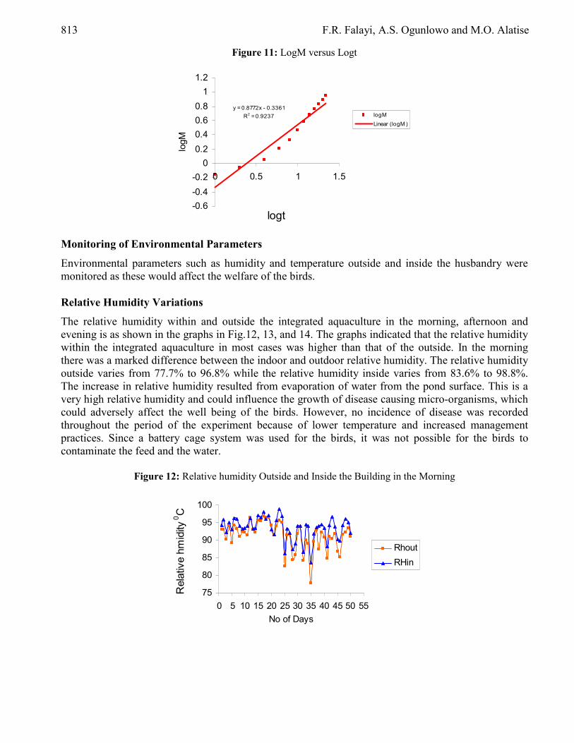
813 F.R. Falayi, A.S. Ogunlowo and M.O. Alatise
Figure 11: LogM versus Logt
y = 0.8772x - 0.3361R2 = 0.9237
-0.6-0.4-0.2
00.20.40.60.8
11.2
0 0.5 1 1.5
logt
logM
logMLinear (logM )
Monitoring of Environmental Parameters
Environmental parameters such as humidity and temperature outside and inside the husbandry were monitored as these would affect the welfare of the birds. Relative Humidity Variations
The relative humidity within and outside the integrated aquaculture in the morning, afternoon and evening is as shown in the graphs in Fig.12, 13, and 14. The graphs indicated that the relative humidity within the integrated aquaculture in most cases was higher than that of the outside. In the morning there was a marked difference between the indoor and outdoor relative humidity. The relative humidity outside varies from 77.7% to 96.8% while the relative humidity inside varies from 83.6% to 98.8%. The increase in relative humidity resulted from evaporation of water from the pond surface. This is a very high relative humidity and could influence the growth of disease causing micro-organisms, which could adversely affect the well being of the birds. However, no incidence of disease was recorded throughout the period of the experiment because of lower temperature and increased management practices. Since a battery cage system was used for the birds, it was not possible for the birds to contaminate the feed and the water.
Figure 12: Relative humidity Outside and Inside the Building in the Morning
75
80
85
90
95
100
0 5 10 15 20 25 30 35 40 45 50 55No of Days
Rel
ativ
e hm
idity
0 C
RhoutRHin
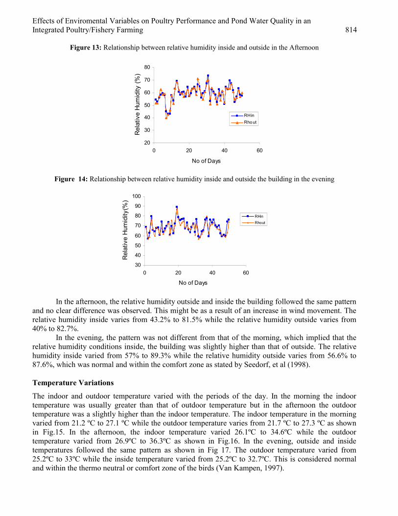
Effects of Enviromental Variables on Poultry Performance and Pond Water Quality in an Integrated Poultry/Fishery Farming 814
Figure 13: Relationship between relative humidity inside and outside in the Afternoon
20
30
40
50
60
70
80
0 20 40 60
No of Days
Rel
ativ
e H
umid
ity (%
)
RHinRhout
Figure 14: Relationship between relative humidity inside and outside the building in the evening
30
40
50
60
70
80
90
100
0 20 40 60
No of Days
Rel
ativ
e H
umid
ity(%
)
RHinRhout
In the afternoon, the relative humidity outside and inside the building followed the same pattern and no clear difference was observed. This might be as a result of an increase in wind movement. The relative humidity inside varies from 43.2% to 81.5% while the relative humidity outside varies from 40% to 82.7%.
In the evening, the pattern was not different from that of the morning, which implied that the relative humidity conditions inside, the building was slightly higher than that of outside. The relative humidity inside varied from 57% to 89.3% while the relative humidity outside varies from 56.6% to 87.6%, which was normal and within the comfort zone as stated by Seedorf, et al (1998). Temperature Variations
The indoor and outdoor temperature varied with the periods of the day. In the morning the indoor temperature was usually greater than that of outdoor temperature but in the afternoon the outdoor temperature was a slightly higher than the indoor temperature. The indoor temperature in the morning varied from 21.2 ºC to 27.1 ºC while the outdoor temperature varies from 21.7 ºC to 27.3 ºC as shown in Fig.15. In the afternoon, the indoor temperature varied 26.1ºC to 34.6ºC while the outdoor temperature varied from 26.9ºC to 36.3ºC as shown in Fig.16. In the evening, outside and inside temperatures followed the same pattern as shown in Fig 17. The outdoor temperature varied from 25.2ºC to 33ºC while the inside temperature varied from 25.2ºC to 32.7ºC. This is considered normal and within the thermo neutral or comfort zone of the birds (Van Kampen, 1997).
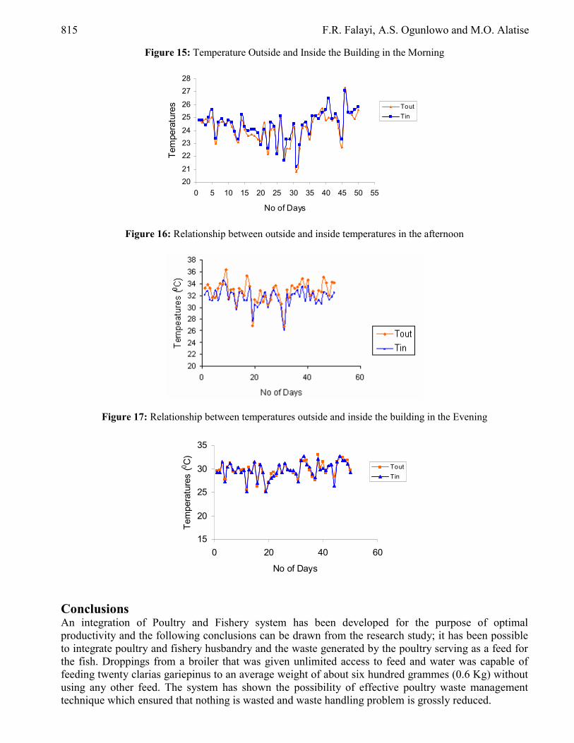
815 F.R. Falayi, A.S. Ogunlowo and M.O. Alatise
Figure 15: Temperature Outside and Inside the Building in the Morning
2021
222324
2526
2728
0 5 10 15 20 25 30 35 40 45 50 55
No of Days
Tem
pera
ture
s ToutTin
Figure 16: Relationship between outside and inside temperatures in the afternoon
Figure 17: Relationship between temperatures outside and inside the building in the Evening
15
20
25
30
35
0 20 40 60
No of Days
Tem
pera
ture
s (0 C
)
ToutTin
Conclusions An integration of Poultry and Fishery system has been developed for the purpose of optimal productivity and the following conclusions can be drawn from the research study; it has been possible to integrate poultry and fishery husbandry and the waste generated by the poultry serving as a feed for the fish. Droppings from a broiler that was given unlimited access to feed and water was capable of feeding twenty clarias gariepinus to an average weight of about six hundred grammes (0.6 Kg) without using any other feed. The system has shown the possibility of effective poultry waste management technique which ensured that nothing is wasted and waste handling problem is grossly reduced.

Effects of Enviromental Variables on Poultry Performance and Pond Water Quality in an Integrated Poultry/Fishery Farming 816
Pollution resulting from the use of poultry droppings adversely affected the development of the fish. Increase in the volume of droppings led to increase in the Bio-Chemical oxygen demand and Chemical Oxygen demand of the pond water which consequently led to a decrease in the dissolved oxygen. Water turbidity also increased with increased droppings. Other water parameters like conductivity, chloride and pH values were within acceptable values suggested in literatures. References [1] Chakrabarty R. D. & A. Hettiarachchi (1982). ‘Preliminary Observations on Fish Polyculture
cum Duck raising in a Farm Pond in Sri Lanka’, Jour Inland Fish. Sri Lanka, Vol 1. 54–61. [2] Chandrasoma J. (1988). Observations on Marketing of fish produced in seasonal tanks', Jour
Inland Fish Sri Lanka, 4: 63–67. [3] Charles D.R. (1994). Comparative climatic requirements. In: Livestock Housing (Wathes C.M;
Carles D.R. eds) CAB international.pp. 3-24. [4] CIGR (1984). Climatisation of animal houses. Report of working group. Scottish Farm building
Investigation Unit, cribastone, Aberdeen, Scotland. [5] Eikmeier H., Mayer H. (1965). The economic importance of the enzootic pneumonia of pigs.
Berliner Munchener Tierartliche Wochenschrift. 78, 449-450. [6] Seedorf J.; Hartung J; Schroder M; Linkert K.H.; Petersen S; Takai H; Johnson J.O.; Metz
J.H.M; Groot P.W.G.; Uenk G.H.; Philips V.R.; Holden M.R.; Sneath R.W. Short J.L.; White R.P. and Wathes C.M.A (1998) Temperature and Moisture conditions in Livestock Buildings in Northern Europe. J. agric Engng Res 70, 49-57
[7] Woynarovich E. (1979). The feasibility of combining animal husbandry with fish farming, with special reference to duck and pig production. In: Advanced in Aquaculture, T. V. R. Pillay and W. A. Dill (eds.). Fishing News Books Ltd. Farnham, Surrey, England, pp. 203–208

European Journal of Scientific Research ISSN 1450-216X Vol.20 No.4 (2008), pp.817-827 © EuroJournals Publishing, Inc. 2008 http://www.eurojournals.com/ejsr.htm
Spatial Distribution and Characterisation of the Sediments of the Estuary of Comoe River (Grand-Bassam, Côte D’ivoire)
Adopo Kouassi Laurent Laboratoire de Géologie Marine, Sédimentologie et Environnement
Centre de Recherche en Ecologie, Université d’Abobo-Adjamé 01 BP 10588 Abidjan 01 (Côte d’Ivoire)
E-mail: [email protected] Tel: (225) 21 25 73 36/08 49 61 00; Fax. (225) 21 24 01 91
Kouassi Kouakou Lazare
Laboratoire de Géologie Marine, Sédimentologie et Environnement Centre de Recherche en Ecologie, Université d’Abobo-Adjamé
01 BP 10588 Abidjan 01 (Côte d’Ivoire) E-mail: [email protected]
Tel: (225) 21 25 73 36/05 61 23 06; Fax. (225) 21 24 01 91
Wognin Ama Valérie Irma Laboratoire de Géologie Marine et Sédimentologie
UFR-Sciences de la Terre et des Ressources Minières Université de Cocody, 22 BP 582 Abidjan 22 (Côte d’Ivoire)
E-mail: [email protected] Tel: (225) 22 48 38 02/07 90 49 62
Monde Sylvain
Laboratoire de Géologie Marine et Sédimentologie UFR-Sciences de la Terre et des Ressources Minières
Université de Cocody, 22 BP 582 Abidjan 22 (Côte d’Ivoire) E-mail: [email protected]
Tel: (225) 22 48 38 02/08 76 75 77
Meledje N’Diaye Hermann Laboratoire de Géologie Marine, Sédimentologie et Environnement
Centre de Recherche en Ecologie, Université d’Abobo-Adjamé 01 BP 10588 Abidjan 01 (Côte d’Ivoire)
E-mail: [email protected] Tel: (225) 21 25 73 36/09 93 96 17; Fax. (225) 21 24 01 91
Aka Kouamé
Laboratoire de Géologie Marine et Sédimentologie UFR-Sciences de la Terre et des Ressources Minières
Université de Cocody, 22 BP 582 Abidjan 22 (Côte d’Ivoire) E-mail: [email protected]
Tel: (225) 22 48 38 02/08 87 30 97
Spatial Distribution and Characterisation of the Sediments of the Estuary of Comoe River (Grand-Bassam, Côte D’ivoire) 818
Abstract
A sedimentological study was carried out at the estuary of Comoe river with the perpose of determining, using the granulometric and mineralogical characteristics, the origin, the transport process and the space distribution of sediments. In the estuary of Comoe river, one distinguishes in the downstream sector a prevalence of mud and fine sands. In the upstream sector sands are mainly middle to coarse in size. The muds are localised in the vicinities of the banks while sands are in the principal channel of the river.
The mineral found in the sediments is characterised by heavy minerals (the amphibole, tourmaline, diopside and epidote) and light minerals (quartz and feldspaths).
The morphoscopy of the quartzs revealed the prevalence of rounded and bright particles, representing a fluviatile transport at a relatively long distance. Keywords: sediment, sand, estuary, Comoe, Grand-Bassam, Côte d’Ivoire
1. Introduction Les estuaires, zones de rencontre entre le fleuve et la mer, présentent une dynamique assez complexe (LE NORMANT, 1995). En effet, les dépôts des particules transportées par les eaux fluviales et marines façonnent la morpho-structure des paysages estuariens.
En Côte d’Ivoire, ABE (1995) et WOGNIN (2004) ont mis en évidence les conséquences de la dynamique de l’embouchure du fleuve Bandama. Celles-ci se traduisent par un déplacement progressif de cette embouchure vers l’Ouest.
Au niveau de l’embouchure de la Comoé à Grand-Bassam, zone de rencontre entre l’Océan Atlantique, la lagune Ebrié et le fleuve Comoé, la dynamique hydrosédimentaire est encore plus spectaculaire si bien que les dépôts successifs de sédiments donnent naissance à un banc de sables qui rompt le contact naturel entre le fleuve et l’océan (KOFFI et al., 1991). Des travaux de dragage ont été effectués pour ouvrir cette embouchure qui s’est toujours refermée quelques années plus tard (TASTET, 1979; ABE et al., 1996; ABE, 2005). Ainsi, des opérations d’ouverture ont respectivement eu lieu en 1987, 1990 et 2005 après les colmatages observés en 1975, 1989 et 2003. Aujourd’hui, cette embouchure reste toujours fermée et entraîne le confinement du milieu estuarien, la surcharge des eaux fluvio-lagunaires et l’envahissement des plans d’eau par les végétaux flottants (SANKARE et ETIEN, 1991; SANKARE et al., 1991). Ces travaux de dragage se sont soldés par des échecs à cause de la non maîtrise de la dynamique sédimentaire qui contrôle le fonctionnement de cette embouchure. Les travaux de ABE et al. (1996) ont révélé que le caractère irrégulier des débits du fleuve Comoé pourrait expliquer, en partie, cette fermeture. En effet, selon ces auteurs, la réduction significative des débits de ce cours d’eau pendant les périodes d’étiage, notamment au cours de ces dernières décennies du fait de l’influence des fluctuations climatiques, favorise les phénomènes de sédimentation. La conjugaison des dépôts fluviatiles et du transit littoral occasionne le colmatage rapide de l’embouchure du fleuve Comoé.
Cependant, ces études ne mettent ni l’accent sur la caractérisation des sédiments du fond au niveau de l’embouchure ni sur la dynamique sédimentaire. Or, l’approche géologique permet de comprendre les multiples variations historiques et de reconstruire les étapes d’évolution de l’environnement (AMEY et al., 2007).
L’objectif de cette étude est de caractériser les sédiments déposés à l’estuaire du fleuve Comoé afin de connaître leur origine, leur mode de transport et leur répartition spatiale.
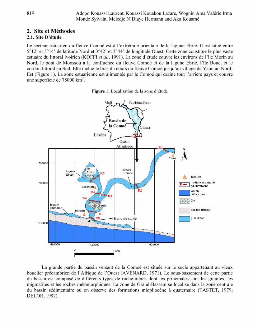
819 Adopo Kouassi Laurent, Kouassi Kouakou Lazare, Wognin Ama Valérie Irma Monde Sylvain, Meledje N’Diaye Hermann and Aka Kouamé
2. Site et Méthodes 2.1. Site D’étude
Le secteur estuarien du fleuve Comoé est à l’extrémité orientale de la lagune Ebrié. Il est situé entre 5°12’ et 5°14’ de latitude Nord et 3°42’ et 3°44’ de longitude Ouest. Cette zone constitue le plus vaste estuaire du littoral ivoirien (KOFFI et al., 1991). La zone d’étude couvre les environs de l’île Morin au Nord, le pont de Moossou à la confluence du fleuve Comoé et de la lagune Ebrié, l’île Bouet et le cordon littoral au Sud. Elle inclue le bras du cours du fleuve Comoé jusqu’au village de Yaou au Nord-Est (Figure 1). La zone estuarienne est alimentée par le Comoé qui draine tout l’arrière pays et couvre une superficie de 78000 km2.
Figure 1: Localisation de la zone d’étude
Banc de sable
Burkina-Faso Mali
Libéria
Ghana
Océan Atlantique
Bassin de la Comoé
La grande partie du bassin versant de la Comoé est située sur le socle appartenant au vieux bouclier précambrien de l’Afrique de l’Ouest (AVENARD, 1971). Le sous-bassement de cette partie du bassin est composé de différents types de roche-mères dont les principales sont les granites, les migmatites et les roches métamorphiques. La zone de Grand-Bassam se localise dans la zone centrale du bassin sédimentaire où on observe des formations miopliocène à quaternaire (TASTET, 1979; DELOR, 1992).

Spatial Distribution and Characterisation of the Sediments of the Estuary of Comoe River (Grand-Bassam, Côte D’ivoire) 820
Les travaux de PERRAUD (1971) ont permis de distinguer différents types de sols sur le bassin de la Comoé. Les formations pédologiques les plus prépondérantes sont les sols ferrallitiques parsemés de quelques lambeaux de sols bruns eutrophes tropicaux dérivés de roches basiques.
Le régime hydrologique du fleuve Comoé est caractérisé par le régime tropical de transition au Nord, le régime tropical de transition atténué au Centre et le régime équatorial de transition au Sud. Les écoulements observés au Sud du bassin de la Comoé sont fortement influencés par le régime tropical de transition du Nord. Ce régime comporte généralement une seule période de hautes eaux (août-septembre-octobre), suivie d’un tarissement rapide de novembre à décembre. 2.2. Méthodes D’étude
Pour déterminer les caractéristiques granulométriques des sables de l’estuaire du fleuve Comoé, 24 échantillons de sédiments ont été prélevés sur huit (8) radiales allant d’une berge à une autre à l’aide d’une benne Van Veen (voir figure 1).
Les sédiments ont été traités selon la technique décrite par SAAIDI (1991). Les matières organiques et les débris coquilliers ont été éliminés respectivement à l’aide de l’eau oxygénée 30% et de l’acide chlorhydrique 50%. Après élimination de la fraction inférieure à 63 µm, chaque échantillon de sable a subi une analyse granulométrique à sec sur une colonne de 16 tamis (série AFNOR). Les sables de l’estuaire ont été caractérisés à travers la moyenne granulométrique (Mz), le skwness (Sk) et l’indice de classement (So), déterminés à l'aide des méthodes de FRIEDMAN (1967) et FOLK (1974).
Les cartes sédimentologiques et les cartes de positionnement ont été réalisées à l’aide des logiciels ArcView 3.3 et SURFER 8.2. 3. Résultats et Discussion 3.1. Description et cartographie des faciès sédimentaires superficiels
3.1.1. Description des faciès sédimentaires L’analyse granulométrique des sédiments superficiels de l’estuaire du fleuve Comoé met en évidence trois faciès lithologiques. Il s’agit des sables, des vases et des sédiments "mixtes" (Tableau I).
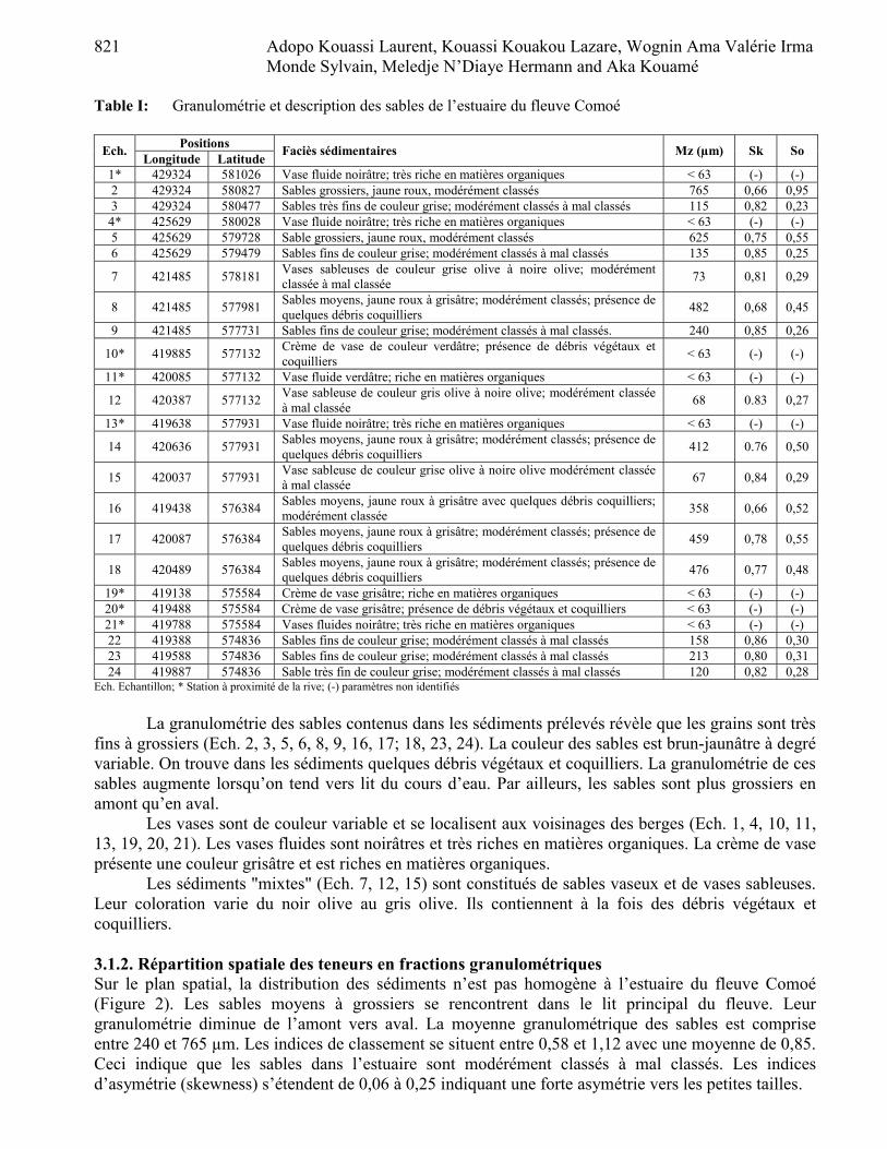
821 Adopo Kouassi Laurent, Kouassi Kouakou Lazare, Wognin Ama Valérie Irma Monde Sylvain, Meledje N’Diaye Hermann and Aka Kouamé
Table I: Granulométrie et description des sables de l’estuaire du fleuve Comoé
Positions Ech. Longitude Latitude Faciès sédimentaires Mz (µm) Sk So
1* 429324 581026 Vase fluide noirâtre; très riche en matières organiques < 63 (-) (-) 2 429324 580827 Sables grossiers, jaune roux, modérément classés 765 0,66 0,95 3 429324 580477 Sables très fins de couleur grise; modérément classés à mal classés 115 0,82 0,23 4* 425629 580028 Vase fluide noirâtre; très riche en matières organiques < 63 (-) (-) 5 425629 579728 Sable grossiers, jaune roux, modérément classés 625 0,75 0,55 6 425629 579479 Sables fins de couleur grise; modérément classés à mal classés 135 0,85 0,25
7 421485 578181 Vases sableuses de couleur grise olive à noire olive; modérément classée à mal classée 73 0,81 0,29
8 421485 577981 Sables moyens, jaune roux à grisâtre; modérément classés; présence de quelques débris coquilliers 482 0,68 0,45
9 421485 577731 Sables fins de couleur grise; modérément classés à mal classés. 240 0,85 0,26
10* 419885 577132 Crème de vase de couleur verdâtre; présence de débris végétaux et coquilliers < 63 (-) (-)
11* 420085 577132 Vase fluide verdâtre; riche en matières organiques < 63 (-) (-)
12 420387 577132 Vase sableuse de couleur gris olive à noire olive; modérément classée à mal classée 68 0.83 0,27
13* 419638 577931 Vase fluide noirâtre; très riche en matières organiques < 63 (-) (-)
14 420636 577931 Sables moyens, jaune roux à grisâtre; modérément classés; présence de quelques débris coquilliers 412 0.76 0,50
15 420037 577931 Vase sableuse de couleur grise olive à noire olive modérément classée à mal classée 67 0,84 0,29
16 419438 576384 Sables moyens, jaune roux à grisâtre avec quelques débris coquilliers; modérément classée 358 0,66 0,52
17 420087 576384 Sables moyens, jaune roux à grisâtre; modérément classés; présence de quelques débris coquilliers 459 0,78 0,55
18 420489 576384 Sables moyens, jaune roux à grisâtre; modérément classés; présence de quelques débris coquilliers 476 0,77 0,48
19* 419138 575584 Crème de vase grisâtre; riche en matières organiques < 63 (-) (-) 20* 419488 575584 Crème de vase grisâtre; présence de débris végétaux et coquilliers < 63 (-) (-) 21* 419788 575584 Vases fluides noirâtre; très riche en matières organiques < 63 (-) (-) 22 419388 574836 Sables fins de couleur grise; modérément classés à mal classés 158 0,86 0,30 23 419588 574836 Sables fins de couleur grise; modérément classés à mal classés 213 0,80 0,31 24 419887 574836 Sable très fin de couleur grise; modérément classés à mal classés 120 0,82 0,28
Ech. Echantillon; * Station à proximité de la rive; (-) paramètres non identifiés
La granulométrie des sables contenus dans les sédiments prélevés révèle que les grains sont très fins à grossiers (Ech. 2, 3, 5, 6, 8, 9, 16, 17; 18, 23, 24). La couleur des sables est brun-jaunâtre à degré variable. On trouve dans les sédiments quelques débris végétaux et coquilliers. La granulométrie de ces sables augmente lorsqu’on tend vers lit du cours d’eau. Par ailleurs, les sables sont plus grossiers en amont qu’en aval.
Les vases sont de couleur variable et se localisent aux voisinages des berges (Ech. 1, 4, 10, 11, 13, 19, 20, 21). Les vases fluides sont noirâtres et très riches en matières organiques. La crème de vase présente une couleur grisâtre et est riches en matières organiques.
Les sédiments "mixtes" (Ech. 7, 12, 15) sont constitués de sables vaseux et de vases sableuses. Leur coloration varie du noir olive au gris olive. Ils contiennent à la fois des débris végétaux et coquilliers. 3.1.2. Répartition spatiale des teneurs en fractions granulométriques Sur le plan spatial, la distribution des sédiments n’est pas homogène à l’estuaire du fleuve Comoé (Figure 2). Les sables moyens à grossiers se rencontrent dans le lit principal du fleuve. Leur granulométrie diminue de l’amont vers aval. La moyenne granulométrique des sables est comprise entre 240 et 765 µm. Les indices de classement se situent entre 0,58 et 1,12 avec une moyenne de 0,85. Ceci indique que les sables dans l’estuaire sont modérément classés à mal classés. Les indices d’asymétrie (skewness) s’étendent de 0,06 à 0,25 indiquant une forte asymétrie vers les petites tailles.
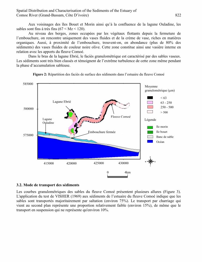
Spatial Distribution and Characterisation of the Sediments of the Estuary of Comoe River (Grand-Bassam, Côte D’ivoire) 822
Aux voisinages des îles Bouet et Morin ainsi qu’à la confluence de la lagune Ouladine, les sables sont fins à très fins (67 < Mz < 120).
Au niveau des berges, zones occupées par les végétaux flottants depuis la fermeture de l’embouchure, on rencontre uniquement des vases fluides et de la crème de vase, riches en matières organiques. Aussi, à proximité de l’embouchure, trouvent-on, en abondance (plus de 80% des sédiments) des vases fluides de couleur noire olive. Cette zone constitue ainsi une vasière interne en relation avec les apports du fleuve Comoé.
Dans le bras de la lagune Ebrié, le faciès granulométrique est caractérisé par des sables vaseux. Les sédiments sont très bien classés et témoignent de l’extrême turbulence de cette zone même pendant la phase d’accumulation sableuse.
Figure 2: Répartition des faciès de surface des sédiments dans l’estuaire du fleuve Comoé
0 4km
< 63 63 - 250250 - 500> 500
Légende
415000 420000 425000 430000
575000
580000
585000
Ile morin Ile bouet Banc de sable Océan
Lagune Ouladine
Fleuve Comoé
Embouchure fermée
Lagune Ebrié
Moyenne granulométrique (µm)
3.2. Mode de transport des sédiments
Les courbes granulométriques des sables du fleuve Comoé présentent plusieurs allures (Figure 3). L'application du test de VISHER (1969) aux sédiments de l’estuaire du fleuve Comoé indique que les sables sont transportés majoritairement par saltation (environ 75%). Le transport par charriage qui vient au second plan représente une proportion relativement faible (environ 15%), de même que le transport en suspension qui ne représente qu'environ 10%.
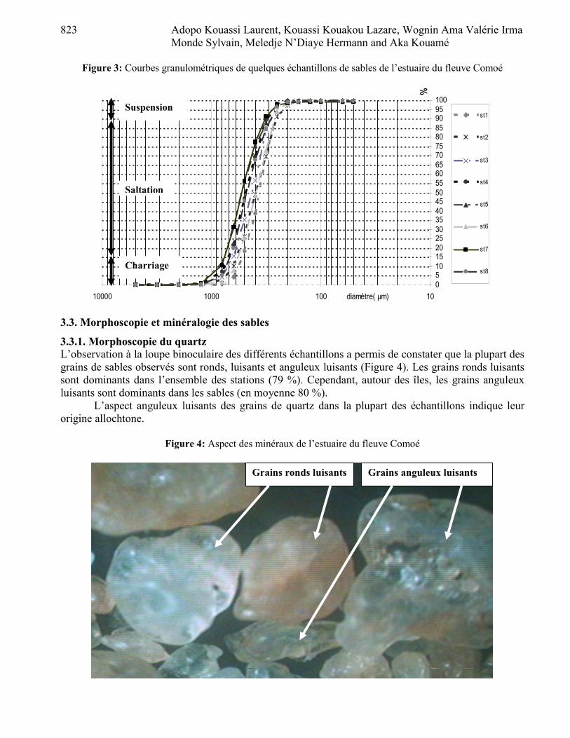
823 Adopo Kouassi Laurent, Kouassi Kouakou Lazare, Wognin Ama Valérie Irma Monde Sylvain, Meledje N’Diaye Hermann and Aka Kouamé
Figure 3: Courbes granulométriques de quelques échantillons de sables de l’estuaire du fleuve Comoé
05101520253035404550556065707580859095100
10100100010000 diamètre( µm)
%
st1
st2
st3
st4
st5
st6
st7
st8
Suspension
Saltation
Charriage
3.3. Morphoscopie et minéralogie des sables
3.3.1. Morphoscopie du quartz L’observation à la loupe binoculaire des différents échantillons a permis de constater que la plupart des grains de sables observés sont ronds, luisants et anguleux luisants (Figure 4). Les grains ronds luisants sont dominants dans l’ensemble des stations (79 %). Cependant, autour des îles, les grains anguleux luisants sont dominants dans les sables (en moyenne 80 %).
L’aspect anguleux luisants des grains de quartz dans la plupart des échantillons indique leur origine allochtone.
Figure 4: Aspect des minéraux de l’estuaire du fleuve Comoé
Grains ronds luisants Grains anguleux luisants
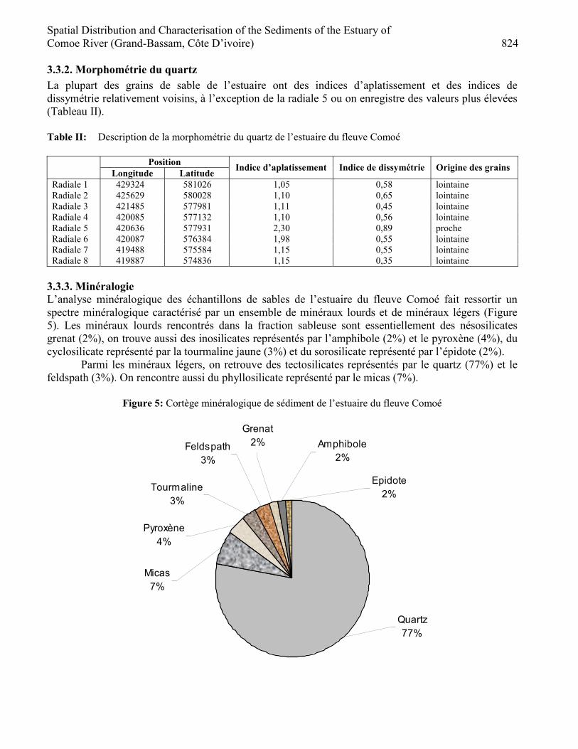
Spatial Distribution and Characterisation of the Sediments of the Estuary of Comoe River (Grand-Bassam, Côte D’ivoire) 824 3.3.2. Morphométrie du quartz La plupart des grains de sable de l’estuaire ont des indices d’aplatissement et des indices de dissymétrie relativement voisins, à l’exception de la radiale 5 ou on enregistre des valeurs plus élevées (Tableau II). Table II: Description de la morphométrie du quartz de l’estuaire du fleuve Comoé
Position Longitude Latitude Indice d’aplatissement Indice de dissymétrie Origine des grains
Radiale 1 429324 581026 1,05 0,58 lointaine Radiale 2 425629 580028 1,10 0,65 lointaine Radiale 3 421485 577981 1,11 0,45 lointaine Radiale 4 420085 577132 1,10 0,56 lointaine Radiale 5 420636 577931 2,30 0,89 proche Radiale 6 420087 576384 1,98 0,55 lointaine Radiale 7 419488 575584 1,15 0,55 lointaine Radiale 8 419887 574836 1,15 0,35 lointaine
3.3.3. Minéralogie L’analyse minéralogique des échantillons de sables de l’estuaire du fleuve Comoé fait ressortir un spectre minéralogique caractérisé par un ensemble de minéraux lourds et de minéraux légers (Figure 5). Les minéraux lourds rencontrés dans la fraction sableuse sont essentiellement des nésosilicates grenat (2%), on trouve aussi des inosilicates représentés par l’amphibole (2%) et le pyroxène (4%), du cyclosilicate représenté par la tourmaline jaune (3%) et du sorosilicate représenté par l’épidote (2%).
Parmi les minéraux légers, on retrouve des tectosilicates représentés par le quartz (77%) et le feldspath (3%). On rencontre aussi du phyllosilicate représenté par le micas (7%).
Figure 5: Cortège minéralogique de sédiment de l’estuaire du fleuve Comoé
Quartz77%
Micas7%
Pyroxène4%
Epidote2%
Amphibole2%
Tourmaline3%
Feldspath3%
Grenat2%

825 Adopo Kouassi Laurent, Kouassi Kouakou Lazare, Wognin Ama Valérie Irma Monde Sylvain, Meledje N’Diaye Hermann and Aka Kouamé
4. Discussion Les analyses granulométriques et minéralogiques montrent que la distribution des sédiments n’est pas homogène dans l’estuaire de la Comoé. Les vases et les sables fins se localisent aux voisinages des îles et des berges, zones fortement colonisées par les végétaux aquatiques envahissants. La présence de vases sur les berges peut s’expliquer par la décomposition suivie de la sédimentation des végétaux aquatiques et de la végétation en bordure du cours d’eau. Par ailleurs, les vitesses des courants qui sont relativement faibles sur les berges favorisent la décantation des matières organiques.
La localisation des sables moyens et grossiers dans le lit du fleuve Comoé peut s'expliquer par l'énergie du courant qui paraît relativement plus importante dans cet axe dont la pente est plus accentuée que les autres parties du fleuve. Dans la partie amont de l’estuaire et notamment dans le bras du fleuve (vers yaou), les sables sont plus grossiers qu’en aval (vers l’embouchure). En effet, la fermeture de l’embouchure crée un plan d’eau où les actions hydrodynamiques sont relativement faibles. KOUASSI (2007) et KOUASSI et al. (2007) rapportent qu’à l’entrée des plans d’eau les éléments grossiers se déposent à la suite d’une diminution de la compétence du transport des cours d’eau.
L’analyse minéralogique des sables révèle la présence de minéraux lourds tels l’amphibole (actinote, hornblende), le rutile, la limonite, le diopside et le zircon. La présence de minéraux légers, notamment le quartz et les feldspaths, dans chaque sédiment est aussi remarquable. Ces minéraux font partie de ceux décrits par BROCHE et al. (1977) dans la partie supérieure du bassin versant du fleuve Comoé. La répartition des minéraux révèle une origine continentale détritique issue des formations de l'arrière-pays.
L’examen morphoscopique montre l’omniprésence des grains arrondis luisants dans l’ensemble de l’estuaire. Ce qui met en évidence l’influence du transport par l’eau des sédiments et de la dynamique fluviale. Les valeurs des différents indices d’aplatissement et de dissymétrie montrent que les grains de sables rencontrés dans l’estuaire ont subi un transport fluviatile sur une longue distance. Ce qui confirme les résultats de l’étude morphoscopique. Toutefois, les échantillons prélevés aux voisinages de l’île Morin (radiale 5) sont anguleux et ont leurs indices d’aplatissement et de dissymétrie élevés. Ce qui montre ces sables sont issus de l’altération des roches en place. 5. Conclusion Les analyses granulométrique et minéralogique ont montré que les sédiments rencontrés dans l’estuaire du fleuve Comoé sont constitués de vases, de sables fins, de sables moyens et de sables grossiers. Ces sables sont majoritairement moyens à grossiers en amont de l’estuaire et fins à très fins vers l’embouchure.
L’aspect arrondi et luisant des grains de sables dans la plupart des échantillons prélevés montre que les sables rencontrés dans l’estuaire proviennent de la partie amont du bassin et ont été transportés sur une distance relativement longue par l’eau.
Le cortège minéralogique renferme à la fois des minéraux lourds tels que l’amphibole (actinote, hornblende), la tourmaline, le diopside et l’épidote et des minéraux légers parmi lesquels le quartz est le plus abondant. Cette étude a montré que la distribution des sédiments n’est pas homogène dans l’estuaire du fleuve Comoé. Les vases et les sables fins se retrouvent du aux voisinages des berges et près de l’île Bouet représentant les zones fortement occupées par les végétaux aquatiques envahissants.
Les travaux se poursuivent dans le but d’étudier les facteurs influençant la répartition spatiale des sédiments dans l’estuaire du fleuve Comoé et prévoir l’évolution, à moyen et long terme, des phénomènes de sédimentation. Les résultats devraient permettre de simuler, à terme, le fonctionnement hydrosédimentaire de l’embouchure du fleuve Comoé.

Spatial Distribution and Characterisation of the Sediments of the Estuary of Comoe River (Grand-Bassam, Côte D’ivoire) 826 6. Remerciements Cette recherche a fait l’objet d’un soutien financier et logistique de la Fondation Internationale pour la Science (IFS, Suède). Nous adressons nos sincères remerciements à cette institution pour sa contribution à nos travaux. References [1] ABE J. (1995). Etude comparative de la dynamique sédimentaire aux embouchures des fleuves
du littoral ivoirien. Proc. Int. Conf. “Costal change 95“ Bordomer-IOC, Bordeaux: 347-363. [2] ABE J. (2005). Contribution à la connaissance de la morphologie et de la dynamique
sédimentaire du littoral Ivoirien (cas du littoral d’Abidjan): Essais de modélisation en vue d’une gestion rationnelle, Thèse de doctorat d’Etat Sc. Nat. Abidjan. 309p.
[3] ABE J., BAKAYORO S., BAMBA S., CISSOKO S. (1996). L’hydrologie de l’estuaire du Comoé à Grand-Bassam (Côte d’Ivoire) Agronomie Africaine. Journal ivoirien d’océanologie et de liminologie. 8 (3): 201-212.
[4] AMEY K. B., BEDJA K., NEGLO K. (2007). Distribution longitudinale de la granulométrie du sable littorale togolais: grain moyen, sorting index et skewness. Journal des Sciences pour l’Ingénieur. N°8: 1 - 8.
[5] AVENARD J.M. (1971). Aspect de la géomorphologie. in: "Le milieu naturel de Côte d’Ivoire", mém. ORSTOM, Paris, n° 50: 1-72.
[6] BROCHE., CASSANOVA R., LOUP G. (1977). Atlas des minéraux en grain Identification par photographies en couleurs, 171 pp.
[7] DELOR C., DIABY et TASTET J-P. (1992). Notice explicative de la carte géologique de la Côte d’Ivoire à 1/200.000, feuille Grand-Bassam, mémoire de la Direction de la géologie de Côte d’Ivoire, n°4, Abidjan Côte d’Ivoire.
[8] FOLK R. L. (1974). Petrology of sedimentary rocks. Austin, Texas: Hemphills, 182 P. [9] FRIEDMAN G. M. (1967). Dynamic processes and statistical parameters compared for size
frequency distribution of beach and river sands. Journal of Sedimentary petrology 37(2): 327-354.
[10] KOFFI. K & ABE J. (1991). Contribution à l’étude des modifications hydro-sédimentaires consécutives à la réouverture artificielle de l’embouchure du Comoé à Grand-Bassam. Journal Ivoirien d’Océanologie et Limnologie: Vol. 1, n°2, 47-60.
[11] KOUASSI K. L. 2007. Hydrologie, transport solide et modélisation de la sédimentation dans les lacs des barrages hydro-électriques de Côte d’Ivoire: cas du lac de Taabo (Côte d’Ivoire). Thèse de doctorat, Univ. d’Abobo-Adjamé, 209p.
[12] KOUASSI K. L., Wognin A. V. I., Gnagne T., N’go Y. A., Courivaud J-R, Kassy P., Demé M. & Aka K., 2007. Caractérisation des sables et morphologie du fond du lac du barrage hydroélectrique de Taabo (Côte d’Ivoire). Science & Nature, 4(1): 93-103.
[13] LE NORMANT C. (1995). Modélisation numérique tridimensionnelle des processus de transport des sédiments cohésifs en environnement estuarien. Thèse de doctorat, Institut National Polytechnique de Toulouse; spécialité physique et chimie de l’environnement. N°1002, 253p.
[14] PERRAUD A. (1971). Les sols. in: "Le milieu naturel de Côte d’Ivoire". Mém. ORSTOM, Paris, n°50: 265-391.
[15] SAAIDI E. (1991). Traité de sédimentologie. Pétrographie, environnements sédimentaires. Edition Ellipes, 393p.
[16] SANKARE Y., ETIEN N. (1991). Analyse des effets de l’ouverture du chenal de Grand Bassam (estuaire du fleuve Comoé, Lagune Ebrié) sur la macrofaune benthique lagunaire. Journal Ivoirien d’Océanologie et Limnologie, 1 (2): 81-90.

827 Adopo Kouassi Laurent, Kouassi Kouakou Lazare, Wognin Ama Valérie Irma Monde Sylvain, Meledje N’Diaye Hermann and Aka Kouamé
[17] SANKARE Y., KOTHIAS A. J-B., KONAN A. A. (1991). Les effets de la réouverture de l’embouchure du fleuve Comoé sur la végétation littorale lagunaire (Lagune Ebrié – Côte d’Ivoire). Journal Ivoirien d’Océanologie et Limnologie, 1 (2): 71-79.
[18] TASTET J. P. (1979): Environnements sédimentaires et structuraux quaternaires du littoral du Golfe de Guinée (Côte d’Ivoire, Togo et Bénin). Thèse de doctorat, Univ. Bordeaux I, n°621, 175p.
[19] VISHER G.S. (1969). Grain-size distributions and depositional processes. Journal of Sedimentary Petrology 39(3): 1074-1106.
[20] WOGNIN A. V. I. (2004). Caractérisation hydrologique et sédimentologique de l’embouchure du fleuve Bandama. Thèse de doctorat, Univ. de Cocody, 198p.
European Journal of Scientific Research ISSN 1450-216X Vol.20 No.4 (2008), pp.828-835 © EuroJournals Publishing, Inc. 2008 http://www.eurojournals.com/ejsr.htm
Blind SIMO GSM Channel Identification
Taba Mohamed Tahar LAIG Laboratory, Guelma University, Algeria
E-mail: [email protected]
S. Femmame LACSC Laboratory, ECE Paris, France
D. Mossadeg
Electronic Department, Annaba University, Algeria
Abstract
The bandwidth efficiency of many communication systems could be improved if the transmission channel was estimated blindly, i.e. without resort to training sequences. GMSK is a spectrum-efficient modulation scheme, and it is adopted as the modulation standard of GSM systems. However, because of its phase modulation, Gaussian filtering, and partial response signalling properties, GMSK is not a linear modulation. Linear approximation of the GMSK signal makes the blind equalization system model applicable for GSM. In this paper, we present a linear approximation of GMSK signals and we propose a blind GSM channel identification algorithm based on the cross relation method. Keywords: GMSK modulation, blind identification, GSM channels, SIMO system.
1. Introduction The Pan-European cellular standard of GSM uses a time division multiple access (TDMA) scheme, where each frequency band is shared by 8 users allocated with 8 time slots. During each time slot (approximately 0.577ms), a 142-bit burst is transmitted, in which two 58-bit streams of information data are separated by a training midamble. The 26-bit training midamble can be used by receivers to identify the unknown linear channel impulse response that includes transmitter filter, physical channel, and receiver filter. This training sequence represents a sizable overhead that reduces the overall system efficiency. If blind /semi-blind equalization [5] can eliminate part of the entire training overhead while maintaining the system performance at an acceptable level, it can significantly improve the system efficiency.
In this study, we first present a new blind channel identification algorithm based on the cross relation method [1]. We note that blind channel identification algorithms based on SOS are sensitive to channel order mismatch [2], which is very common in wireless environment.
The rest of our paper is organized as follows. Section 2 describes an approximated linear model for the nonlinear Gaussian shift keying modulation (GMSK) used in GSM. In section 3, we expose method of extracting channel diversity from linear GMSK system. In section 4, we introduce the blind channel identification algorithm based on the cross relation. And in section 5, simulation results are presented.

Blind SIMO GSM Channel Identification 829
2. GMSK Approximation The impulse response of the Gaussian LPF h(t) is:
⎟⎟⎠
⎞⎜⎜⎝
⎛ −= 2
2
2exp
2)( t
Bth σ
πσ (1)
Where
2ln2 Bπσ = , with BT = 0.3 for GSM.
B is the 3 dB bandwidth of the filter. The square pulse response g(t) of the Gaussian LPF is:
⎟⎠⎞
⎜⎝⎛=
Ttrectthtg *)()(
Where the rectangular function rect(x) is defined by:
⎪⎩
⎪⎨⎧ <
=⎟⎠⎞
⎜⎝⎛
Otherwise
TtforTTtrect
,02
,1
The pulse response g(t) can be written as
⎥⎥⎦
⎤
⎢⎢⎣
⎡⎟⎟⎠
⎞⎜⎜⎝
⎛ +−⎟⎟⎠
⎞⎜⎜⎝
⎛ −=
)2ln(22
)2ln(22
21)(
TTtBTQ
TTtBTQ
Ttg ππ (2)
Where Q (t) is the Q-function
τπ
τ dtQt∫∞
⎟⎟⎠
⎞⎜⎜⎝
⎛−= 2exp
21)(
2 (3)
Consequently, the continuous phase modulation (CPM) pulse is the integral
∫∞−
−=t
dTgt ττψ )2()( (4)
In GSM system, the GMSK parameter BT=0.3 is chosen so that:
⎩⎨⎧
≥≤
≈.4,1
;0,0)(
Ttt
tψ (5)
The baseband signal of GMSK modulation is:
⎥⎦
⎤⎢⎣
⎡−= ∑
∞
−∞=nn
nTtjts )(2
exp)( ψπ α (6)
In witch 1±=αn is the binary data for transmission. Because, existing blind equalization algorithm rely on linear system models, linear approximation of the GMSK signal becomes the necessary first step. Following the approach used in [1] for linear QAM approximation of the GMSK signal used in GSM, we take the first approximation step:
⎥⎦
⎤⎢⎣
⎡−= ∑
∞
−∞=nn nTtjts )(
2exp)( ψπ α ∏∑
−=
−
−∞=⎥⎦⎤
⎢⎣⎡ −⎟
⎠
⎞⎜⎝
⎛≈
n
nkk
n
kk kTtjj
3
4
)(2
exp2
exp ψππ αα (7)
t Є [nT, (n+1)T). Equation (7) becomes the basis of linear approximation. It can be seen that there are 16
different terms in the product expansion of (7). Among the 16 different linear pulses, however, only two pulses are significant while the others are nearly all zero. Retaining these two most significant pulses, the linear approximate model for GMSK with BT = 0.3 is:
)()()( 1,10,0 nTtnTtts hahan
nn
n −+−= ∑∑∞
−∞=
∞
−∞=
(8)
Where

830 Taba Mohamed Tahar, S. Femmame and D. Mossadeg
aa nn
n
nnn
jj1,0,0 2
exp−
−∞=
=⎥⎦
⎤⎢⎣
⎡= ∑ ααπ
a nnn 2,01 −−−= αα
aa nn
n
nnnn
jjj2,0,1 2
exp−
−∞=
=⎥⎦
⎤⎢⎣
⎡= ∑ ααα π
In other words, the GMSK signal can be approximated with almost no error by the sum of two QAM signals with pulse shapes h0(t) and h1(t). These two pulses in the linear approximation [3], are shown in figure 1.
For the case L = 4, BT=0.3, )()2()3()4()(0 TtTtTtTtth −−−−= ββββ (9)
0 ≤ t≤ 5T )()4()2()()(1 TtTtTtTtth +−−−= ββββ (10)
0 ≤ t ≤ 3T With,
⎪⎪⎪
⎩
⎪⎪⎪
⎨
⎧
≥
−
−
=
0,0]0,(),(
),0[,)sin(
)](sin[
)(t
LTtt
LTth
thh
t εβ
επ
ψππ
β (11)
With h=0.5 β(t) becomes:
⎪⎩
⎪⎨
⎧
≥
−=
0,0]0,(),(
),0[))(cos()(
2
tLTtt
LTttgt εβ
εβ
π
πσσσ
σσψ
22)2/exp()2/exp(
...2
)()(21
)(
22
221
2
2211
p
p
Ttt
TtQttQt
t
−−−−
−−
+= (12)
,21pTtt −= ,22
pTtt += 2ln2 Bπσ =
Tp: sampling period. Figure 1: Represents two pulse shapes in the GMSK linear approximation. The power in h1(t) is 0.48% of the
power in h0(t).
h0(t)
h1(t)
Because the majority (99.5%) of signal energy in GMSK signal s(t) is contained in the first pulse approximation h0(t) figure 1, we can further simplify s(t) into a single QAM transmission
10 ),()( −
∞
−∞=
=−= ∑ nnnn
n ajanTtts ha α (13)
It can be noted that the approximation error may be viewed as an additive interference. Therefore, even in noiseless channels, the maximum signal-to-noise ratio (SNR) of this approximation
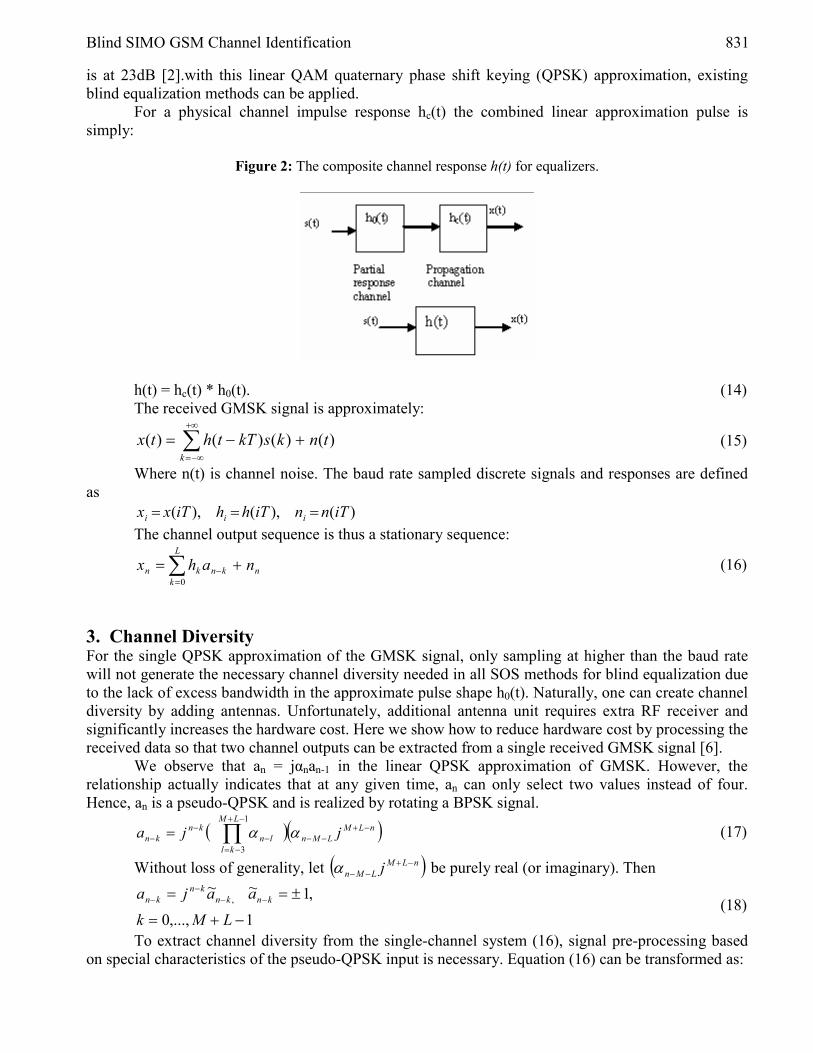
Blind SIMO GSM Channel Identification 831
is at 23dB [2].with this linear QAM quaternary phase shift keying (QPSK) approximation, existing blind equalization methods can be applied.
For a physical channel impulse response hc(t) the combined linear approximation pulse is simply:
Figure 2: The composite channel response h(t) for equalizers.
h(t) = hc(t) * h0(t). (14) The received GMSK signal is approximately:
)()()()( tnkskTthtxk
+−= ∑+∞
−∞=
(15)
Where n(t) is channel noise. The baud rate sampled discrete signals and responses are defined as
)(),(),( iTnniThhiTxx iii === The channel output sequence is thus a stationary sequence:
n
L
kknkn nahx += ∑
=−
0
(16)
3. Channel Diversity For the single QPSK approximation of the GMSK signal, only sampling at higher than the baud rate will not generate the necessary channel diversity needed in all SOS methods for blind equalization due to the lack of excess bandwidth in the approximate pulse shape h0(t). Naturally, one can create channel diversity by adding antennas. Unfortunately, additional antenna unit requires extra RF receiver and significantly increases the hardware cost. Here we show how to reduce hardware cost by processing the received data so that two channel outputs can be extracted from a single received GMSK signal [6].
We observe that an = jαnan-1 in the linear QPSK approximation of GMSK. However, the relationship actually indicates that at any given time, an can only select two values instead of four. Hence, an is a pseudo-QPSK and is realized by rotating a BPSK signal.
( )( )∏−+
−=
−+−−−
−− =
1
3
LM
kl
nLMLMnln
knkn jja αα (17)
Without loss of generality, let ( )nLMLMn j −+
−−α be purely real (or imaginary). Then
1,...,0
,1~~,
−+=
±== −−−
−
LMk
aaja knknkn
kn (18)
To extract channel diversity from the single-channel system (16), signal pre-processing based on special characteristics of the pseudo-QPSK input is necessary. Equation (16) can be transformed as:

832 Taba Mohamed Tahar, S. Femmame and D. Mossadeg
n
L
kkn
knkn ajhx ω+= ∑
=−
−
0
~ [ ] n
L
kkn
knk ajh ω+= ∑
=−
−
0
~ (19)
As a result, we can obtain a new (derotated) sequence:
[ ] nn
L
kkn
kk
nnn
jajh
jxx
ω−
=−
−
−
+=
=
∑0
~
~
(20)
Derotation not only changes the GMSK detection into a simpler BPSK detection problem, it can also create channel diversity useful in blind equalization [1]
Since na~ is real-valued sequence, we can induce two sub-channel outputs from (20):
[ ] [ ]∑=
−−
− +==L
kn
nkn
kknn jajhxx
0
1 Re~Re~Re ω
[ ] [ ]∑=
−−
− +==L
kn
nkn
kknn jajhxx
0
2 Im~Im~Im ω (21)
Where the common input is a BPSK signal, i.e. .1~ ±== −
nn
n aja From the BPSK input data sequence, two sub-channels can be generated without over-sampling
and extra antenna, k
kkk
kk jhhandjhh −− == Im()Re( 21 We hence arrive at the familiar equation in SIMO [7] (Single Input / Multiple Output) models: X[k] = Hã[k] + n[k] Where: [ ]
[ ] ,Im
][Re⎥⎦
⎤⎢⎣
⎡=
kxkx
kx ,
ImRe
⎥⎦
⎤⎢⎣
⎡=
HH
H [ ] [ ] .
Im][Re⎥⎦
⎤⎢⎣
⎡=
knkn
kn (22)
H will have full column rank if )Re( kk jh − and k
k jh −Im( share no common zeros [2]. 4. Cross-Relation Method Consider a SIMO system of q outputs given by:
∑=
+−=M
klnklskhly
0)()()()( (23)
The noise free outputs yi(k), 1≤ i≤ q are given by: yi(k) = hi(k) * s(k), 1≤ i≤ q (24)
where “*” denotes convolution. Using commutativity of convolution, it follows: hj(k) * yi(k) = hi(k) * yj(k), 1≤ i<j≤ q (25) This is a linear equation satisfied by every pairs of channels. It was shown [4] that based on q(q-1)/2 possible cross-correlation, the channel parameters can
be uniquely identified. By collecting all possible pairs of q channels, one can easily establish a set of linear equations.
In matrix form, this set of equations can be expressed as: Yqh =0 (26) Where Yq isdefined by: Y2 = [Y(2), -Y(1)]

Blind SIMO GSM Channel Identification 833
⎥⎥⎥⎥⎥⎥
⎦
⎤
⎢⎢⎢⎢⎢⎢
⎣
⎡
−••••
−
=
−
−
)1()(
)1()(
)1(
0
00
ll
l
l
l
YY
YYY
Y (27)
With l = 3,…,q and:
⎥⎥⎥⎥⎥⎥
⎦
⎤
⎢⎢⎢⎢⎢⎢
⎣
⎡
−−•••−••••••
•••
=
)1()1(
)0()(
)(
MNyNy
yMy
Y
ll
ll
l (28)
In the presence of noise, equation (26) can be naturally solved in the least- square (LS) [4] sense according to:
hYYhh qH
qH
hCR 1minargˆ
== (29)
5. Simultion Results We now present simulation results of GSM blind identification. A GMSK pulse of four symbols was generated and bandwidth BT=0.3. The bit rate is 27 kb/s.
Figure 3: Estimation of propagation channel.
s(t): transmitted signal BPSK n(t): additive noise h(t): combined filter [h(t)=h0(t)*hc(t)] Figure 3 represents the estimated impulse response of the propagation channel for COST-207
[6]. Figure 4 represents the relative error estimation for training method and blind method.
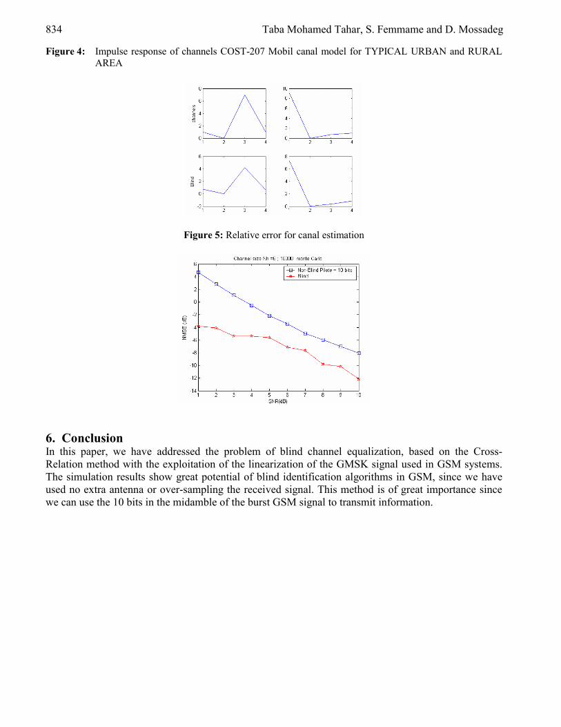
834 Taba Mohamed Tahar, S. Femmame and D. Mossadeg
Figure 4: Impulse response of channels COST-207 Mobil canal model for TYPICAL URBAN and RURAL AREA
Figure 5: Relative error for canal estimation
6. Conclusion In this paper, we have addressed the problem of blind channel equalization, based on the Cross-Relation method with the exploitation of the linearization of the GMSK signal used in GSM systems. The simulation results show great potential of blind identification algorithms in GSM, since we have used no extra antenna or over-sampling the received signal. This method is of great importance since we can use the 10 bits in the midamble of the burst GSM signal to transmit information.

Blind SIMO GSM Channel Identification 835
References [1] Karim Abed-Meraim, Wanzhi Qiu, and Yingbo Hua, “Blind System Identification”,
Proceedings of the IEEE, pp. 1310:1322, AUGUST 1997 [2] Zhi Ding and Ge Li, “Single Channel Blind Equalization for GSM Cellular Systems,” IEEE
Journal on Selected Areas in Communications, Vol. 16, No. 8, Oct. 1998. [3] Ghassan Kawas Kaleh, “Simple Coherent Receivers for Partial Response Continuous Phase
Modulation,” IEEE Journal on Selected Areas in Communications, vol. 7, NO. 9, December 1989
[4] A. Aïssa-El-Bey, M. Grebici, K. Abed-Meraim and A. Belouchrani, “Blind System Identification Using Cross-Relation Methods: Further Results And Developments,” 7th International Symposium on Signal Processing and its Applications (ISSPA), vol. 1, pp. 649-652, Paris, France, July, 2003.
[5] CICHOCKI Andrzej, AMARI Shun-ichi, “Adaptive Blind Signal and Image Processing: Learning Algorithms and Applications”, Willey 2001.
[6] P. Hoeher, “A Statistical Discrete-Time Model for the WSSUS Multipath Channel,” IEEE Transactions on Vehicle Technology, vol.41, pp. 461-468, Nov. 1992.
[7] Jingdong Chen; Nteng Huang; Benesty, J, “An adaptive blind SIMO identification approach to joint multichannel time delay estimation”, Acoustics, Speech, and Signal Processing, 2004. Volume 4, Issue, 17-21 May 2004
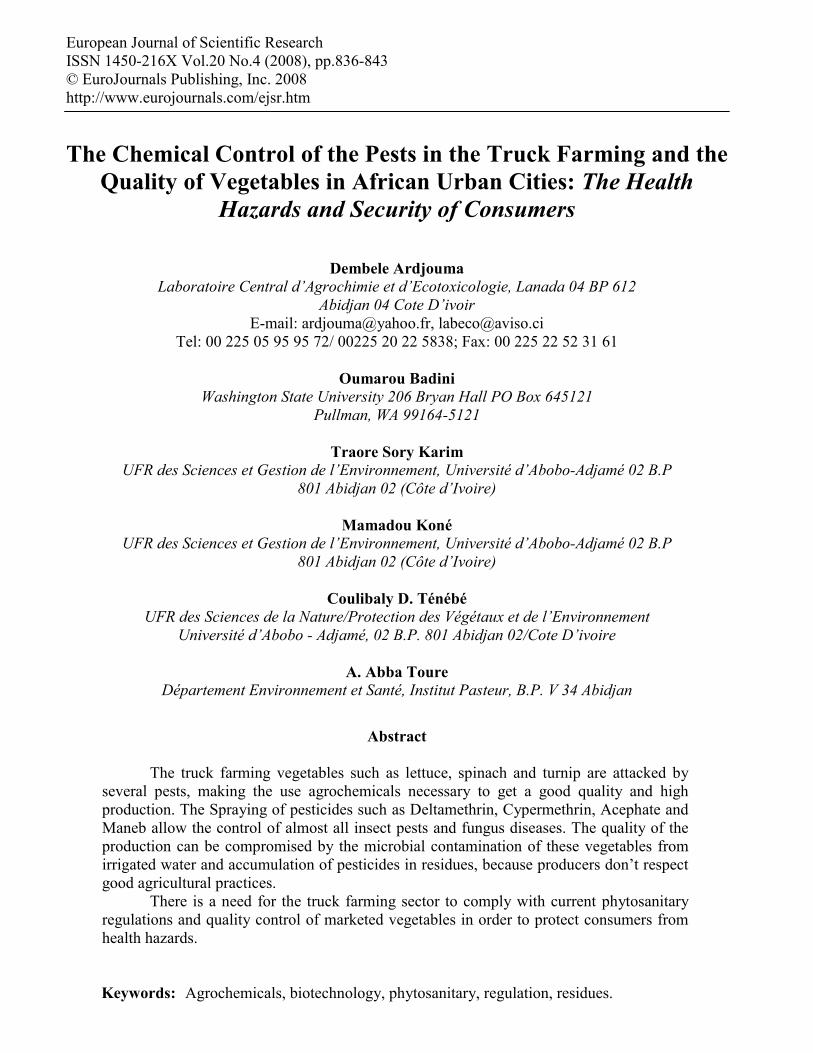
European Journal of Scientific Research ISSN 1450-216X Vol.20 No.4 (2008), pp.836-843 © EuroJournals Publishing, Inc. 2008 http://www.eurojournals.com/ejsr.htm
The Chemical Control of the Pests in the Truck Farming and the
Quality of Vegetables in African Urban Cities: The Health Hazards and Security of Consumers
Dembele Ardjouma Laboratoire Central d’Agrochimie et d’Ecotoxicologie, Lanada 04 BP 612
Abidjan 04 Cote D’ivoir E-mail: [email protected], [email protected]
Tel: 00 225 05 95 95 72/ 00225 20 22 5838; Fax: 00 225 22 52 31 61
Oumarou Badini Washington State University 206 Bryan Hall PO Box 645121
Pullman, WA 99164-5121
Traore Sory Karim UFR des Sciences et Gestion de l’Environnement, Université d’Abobo-Adjamé 02 B.P
801 Abidjan 02 (Côte d’Ivoire)
Mamadou Koné UFR des Sciences et Gestion de l’Environnement, Université d’Abobo-Adjamé 02 B.P
801 Abidjan 02 (Côte d’Ivoire)
Coulibaly D. Ténébé UFR des Sciences de la Nature/Protection des Végétaux et de l’Environnement
Université d’Abobo - Adjamé, 02 B.P. 801 Abidjan 02/Cote D’ivoire
A. Abba Toure Département Environnement et Santé, Institut Pasteur, B.P. V 34 Abidjan
Abstract
The truck farming vegetables such as lettuce, spinach and turnip are attacked by several pests, making the use agrochemicals necessary to get a good quality and high production. The Spraying of pesticides such as Deltamethrin, Cypermethrin, Acephate and Maneb allow the control of almost all insect pests and fungus diseases. The quality of the production can be compromised by the microbial contamination of these vegetables from irrigated water and accumulation of pesticides in residues, because producers don’t respect good agricultural practices.
There is a need for the truck farming sector to comply with current phytosanitary regulations and quality control of marketed vegetables in order to protect consumers from health hazards. Keywords: Agrochemicals, biotechnology, phytosanitary, regulation, residues.
The Chemical Control of the Pests in the Truck Farming and the Quality of Vegetables in African Urban Cities: The Health Hazards and Security of Consumers 837
Introduction Horticulture is a vital economic sector for most African countries. In Côte d’Ivoire, this sector is confronted to pests’ attacks and phytosanitary problems. It needs to comply to the pesticides regulations and the quality control (traceability) which are now required by most industrials and export countries. The study was conducted in the “M’POUTO village” on the surroundings of the Ebrié lagoon in Abidjan, the economic capital of Côte d’Ivoire. The main objective of this study is to assess the impact of pest on truck farming Lettuce, Spinach, and Turnip, and the application of agrochemicals for plant protection, and the quality of irrigation water. The specific objectives are (1) to evaluate the impact of agrochemicals application on plants pests, (2) to determine their economic incidence, (3) to monitor irrigation water quality, and (4) to control some essential production factors which are indicators of a good standard quality production. Materials And Methods Plant material
The Lettuce, Lactuca sativa L. (Asteraceae or Compositaceae) is the more consumed vegetable in the world. There are approximately 149 varieties worldwide [1]. There are two main classes of lettuce: non-head forming lettuces such as the “celtuce” or “lettuce - asparagus” and the head-forming lettuces such as the “Batavia” or “curly” cabbage lettuce.
Seeds germination is normal between 0°C and 25°C, and sunlight plays a major role in the growth and the development process.
Lettuce has a high water demand [2], and grows well in different types of soils presenting a steady structure with good water holding capacity. In general, lettuce is a moderately heavy consumer of nutrients. Seedlings of lettuce are planted at 2 to 4 leaf-stage in well-prepared seedbeds (trays of earth) ploughed at depth and mixed to manure. The application of fertilizer (NPKS) is often necessary and must be incorporated in the soil before planting. The growth cycle is very variable (45 to 100 days) depending on the variety. Agrochemicals applications (insecticides and fungicides) on the lettuce cultures against the pest attacks are often done in the middle and end of cultural cycle.
The spinach, Spinacia oleracea L. (Chénopodiaceae), is named “the prince of vegetables”. It is an annual plant generally cultivated as biennial in the vegetable exploitations gardens. The plant develops initially, on a very short axis, a rosette constituted of fifteen (15) to twenty (20) leaves. These leaves are lengthily petiolate with full limb more or less blighted. Mineral fertilization (NPK) is often necessary according to expected yields. But the poultry’s liquid manures and dejections abundantly brought are very largely sufficient to face exports of mineral elements. Watering must be sufficiently abundant to satisfy the water needs of the plant. The diseases and pest management of the plants must be carefully and frequently controlled so [3], the weedings are very important and a thinning can be practiced in case of a very dense germination and seedlings. Spinach usually matures in 35 to 45 days. The plant may be harvested from the time there are 5-6 leaves on the plant right before the seed stalk develops. The phytosanitary protection of the plants intervenes in middle and end of cycle.
The turnip, Brassica rapa L. var. rapa, (Brassicaceae) is produced in specialized market gardening. The plant is normally bi-annual. In its vegetative stage it is constituted of a basal rosette made of about fifteen leaves with real green limb and bristling with rough hairs.
According to the varietal type, it has a tuberous root of flattened, conical or cylindrical form and of variable color (white, yellow, black or two-tone).
One notes about thirty varieties but the range of the varieties currently cultivated is rather restricted (Tokyo hybridizes F1, Chinese turnip). Turnips are primarily cultivated in full field by direct seeding on fertile well-prepared seedbeds is also possible. The needs in mineral elements are important and sustained fertilization (NPK) is needed before planting and during the growth cycle.

838 Dembele Ardjouma, Oumarou Badini, Traore Sory Karim, Mamadou Koné, Coulibaly D. Ténébé, A. Abba Toure
The application of manure must be done on the precedent crop. The growth cycle is 40 - 70
days dependent on climatic conditions and varieties. Turnips are harvested as young roots by successive thinnings. The diseases control and protection of turnips must be regular due to frequent pest attacks. Agrochemicals material[4]
Deltamethrin: Trade name DECIS (K -OTHRINE) Molecular formula: C22H19Br2NO3 (S)- α-cyano-3-phenoxybenzyl (1R,3R)-3-(2,2-dibromovinyl)-2,2-dimethylcyclopropane
carboxylate (IUPAC) structural formula:
Decis 25 EC is an emulsifiable concentrate of formulation (25g/l). It is approved for a wide
variety of insects including acarina, thysanoptera and arthropods pests of the horticultural plants. We made a first application on the salad lettuce at the stage 27 days with an amount of
treatment of 0.042 g/l (25 l of Decis in 15 l of water) for 400 m2. The stage 39 days: corresponds to the second treatment by Deltamethrin with the same
concentration of 0,042 g/l and by Maneb with the concentration of 5 g/l representing 93,75 grams of CALLIMAN 80 WP for the sprayer of 15 liters for 400 m2.
The stage 45 days: corresponds to the third treatment by Maneb with the same concentration of 5 g/l.
For turnip, at the stage 18 days we have done the first treatment by Deltamethrin with the concentration of 0,025 g/l (15 milliliters of DECIS 25 EC in 15 liters of water) for 400 m2.
The Stage 30 days: corresponds to the second treatment by Deltamethrin with the same concentration of 0,025 g/l and by Maneb with the concentration of 5 g/l representing 93,75 grams of CALLIMAN 80 WP for the sprayer of 15 liters. The Stage 38 days of turnips received the same treatment as the stage 30 days.
Cypermethrin: Trade name Cypercal 50 EC Molecular formula: C22H19C12NO3 (RS)-I-cyano-3-phenoxybenzyl (1RS)-cis-trans-3- (2,2-dichlorovinyl)-2,2-dimethylcyclopropanecarboxylate (IUPAC) Structural formula:
Cypermethrin 50 EC is an emulsifiable concentrate of formulation (50 g/l). It is approved for a
broad spectrum of harmful insects (Caterpillars, Thrips, Heliothis and white flies). We carried out the first application on spinaches at the stage 18 days, the amount of application is of 0.133 g/l (40 ml of CYPERCAL 50 EC. in 15l of water) for 400 m2. At the stage 30 days the spinaches received an

The Chemical Control of the Pests in the Truck Farming and the Quality of Vegetables in African Urban Cities: The Health Hazards and Security of Consumers 839
amount of treatment of 0,133 g/l in addition to 5 g/l of maneb (93.75g of CALLIMAN 80 WP in 15 l of water) for 400 m2.
Acephate : Trade name Orthen 75 SP Molecular formula : C4H10NO3PS O,S-dimethyl acetylphosphoramidothioate (IUPAC) Structural formula:
Orthen 75 SP is a water-soluble powder of formulation 75% acephate. It is a systemic pesticide.
Methadomiphos (C2H8O2NPS) is a metabolite of acephate and it is also systemic. Structural formula: O
" CH3OPSCH3 ' NH2
O,S,-dimethyl phosphoramidothioate (IUPAC) These two organophosphorous pesticides are both effective against a broad range of insect pests
(sucking, biting, and mining insects) on such vegetable and crops as cabbages, cotton, tobacco, sugar beet, head lettuce. It is used as a pre-harvest spray at 0.5-1.5 kg/ha. With this amount, protection against the insects vermin is obtained from 7 to 21 days.
The first application on lettuce is done at at stage 27 days with the amount of 2 g/l (40 g of Orthen 75 SP in 15 l of water) for 400m2.
At the stage 39 days the amount of treatment of lettuce is 2 g/l in addition to 5 g/l of maneb for 400 m2.
Maneb: Trade name Calliman 80 WP Molecular formula: C4H6N2S4Mn Manganese ethylene-1,2-bisdithiocarbamate (IUPAC) Structural formula:
Calliman 80 WP is a wettable powder of formulation 80% of maneb (dithiocarbamate), an
effective protective fungicide against the main foliar diseases(Anthracnose, Mildew, Alternaria, Rhizoctonia, cercospora, Sclerotinia and Septoria).
It should be applied before and after seeding on all three vegetables at amount of 5 g/l. Moreover the salad lettuce received a treatment at the stage of 45 days. Plants phytopathology and pests monitoring
After each treatment, every two (2) days we proceed: • to the description of the general characteristics of the plants, especially the leaves, and we look
out for visible signs of attacks and diseased plants. • to the counting of the insects captured in the traps for follow-up of the dynamics of the
recolonisation following the various treatments[5].
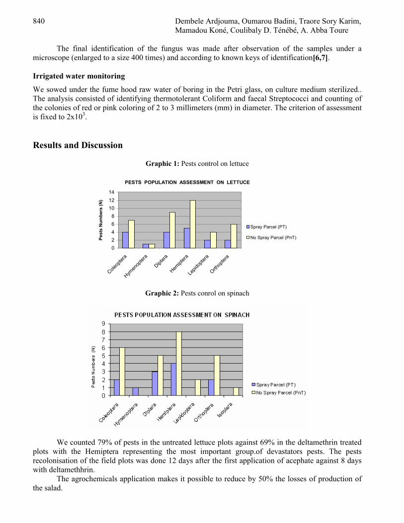
840 Dembele Ardjouma, Oumarou Badini, Traore Sory Karim, Mamadou Koné, Coulibaly D. Ténébé, A. Abba Toure
The final identification of the fungus was made after observation of the samples under a
microscope (enlarged to a size 400 times) and according to known keys of identification[6,7]. Irrigated water monitoring
We sowed under the fume hood raw water of boring in the Petri glass, on culture medium sterilized.. The analysis consisted of identifying thermotolerant Coliform and faecal Streptococci and counting of the colonies of red or pink coloring of 2 to 3 millimeters (mm) in diameter. The criterion of assessment is fixed to 2x10³. Results and Discussion
Graphic 1: Pests control on lettuce
PESTS POPULATION ASSESSMENT ON LETTUCE
02468
101214
Coleop
tera
Hymen
opter
a
Diptera
Hemipt
era
Lepid
opter
a
Orthop
tera
Pest
s N
umbe
rs (N
)
Spray Parcel (PT)
No Spray Parcel (PnT)
Graphic 2: Pests conrol on spinach
We counted 79% of pests in the untreated lettuce plots against 69% in the deltamethrin treated plots with the Hemiptera representing the most important group.of devastators pests. The pests recolonisation of the field plots was done 12 days after the first application of acephate against 8 days with deltamethhrin.
The agrochemicals application makes it possible to reduce by 50% the losses of production of the salad.
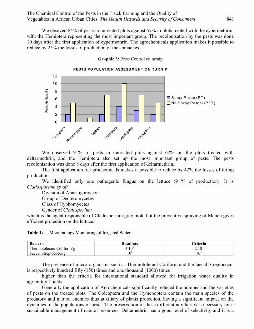
The Chemical Control of the Pests in the Truck Farming and the Quality of Vegetables in African Urban Cities: The Health Hazards and Security of Consumers 841
We obseved 84% of pests in untreated plots against 57% in plots treated with the cypermethrin, with the Hemiptera representing the most important group. The recolonisation by the pests was done 10 days after the first application of cypermethrin. The agrochemicals application makes it possible to reduce by 25% the losses of production of the spinaches.
Graphic 3: Pests Control on turnip
PESTS PO PULAT IO N ASSESS M ENT O N TURNIP
0
2
4
6
8
10
12
Coleop
tera
Hymeno
ptera
Diptera
Hemiptera
Lepid
opter
a
Orthop
tera
Pest
s Nu
mbe
rs (N
)
Spray Pa rce l(PT)No Sp ray Pa rcel (Pn T)
We observed 91% of pests in untreated plots against 62% on the plots treated with deltarmethrin, and the Hemiptera also set up the most important group of pests. The pests recolonisation was done 8 days after the first application of deltarmethrin.
The first application of agrochemicals makes it possible to reduce by 42% the losses of turnip production.
We identified only one pathogenic fungus on the lettuce (9 % of production). It is Cladosporium sp of:
Division of Amastigomycota Group of Deuteromycetes Class of Hyphomycetes Gender of Cladosporium.
which is the agent responsible of Cladosporium gray mold but the preventive spraying of Maneb gives efficient protection on the lettuce. Table 1: Microbiology Monitoring of Irrigated Water
Bacteria Resultats Criteria Thermotolerant Coliform/g 3.105 2.103 Faecal Streptococci/g 106 103
The presence of micro-organisms such as Thermotolerant Coliform and the faecal Streptococci
is respectively hundred fifty (150) times and one thousand (1000) times higher than the criteria for international standard allowed for irrigation water quality in
agricultural fields. Generally the application of Agrochemicals significantly reduced the number and the varieties
of pests on the treated plots. The Coleoptera and the Hymenoptera contain the main species of the predatory and natural enemies thus auxiliary of plants protection, having a significant impact on the dynamics of the populations of pests. The preservation of these different auxiliaries is necessary for a sustainable management of natural resources. Deltamethrin has a good level of selectivity and it is a

842 Dembele Ardjouma, Oumarou Badini, Traore Sory Karim, Mamadou Koné, Coulibaly D. Ténébé, A. Abba Toure
considerable advantage for the management of pests and the environment management than the Acephate which, has a low selectivity but a wide range of effectiveness against insect pest and good residual activity.
The preservation of the auxiliaries of culture in spite of the chemical treatment is essential considering the important role that they play in the maintenance of agro-ecological balances.
The Lepidoptera (larva), Orthoptera and Hemiptera represent the most important group of insect pests, which attack and cause the highest damage in truck farming lettuce, spinach and turnip. However, the considerable differences in number of captured insects and pests found between the treated and untreated field plots show that a targeted application of agrochemicals against these groups of pests is efficient.
The majority of the groups of pests which attach and cause important damage on turnip, spinach and lettuce can be controlled by the application of agrochemical products according to good agricultural practices (GAP) compatible with the protection of the environment and the preservation of non-target organisms.
However, one of the biggest problems encountered by vegetable producers is their lack of sufficient knowledge about how to use safely the agrochemicals. They are not sufficiently aware of the risks of pesticides accumulation in vegetables, and the possible health problems for consumers being exposed to these risks. They are also often confronted with the problems of accessibility to agricultural credits.
The microbiological analysis of the irrigation water highlighted an overload of thermotolerant Coliforms and fecal Streptococci. These bacteria which are not normally pathogenic, are usually used to indicate the possible presence of pathogenic microfauna organisms. Thus their very high number compared to the threshold recommended shows a low water quality.
The strong presence of these indicating bacteria suggests a probable presence in the irrigation water of very dangerous pathogenic parasites that could develop and cause very important damages to the plants, farmers and the consumers.
The contaminated vegetables can cause a certain number of diseases. Particularly, the contaminated salads are sources of bacterial diseases such as the typhoid and paratyphoid fevers (Salmonella typhi/paratyphi) whose origin comes from the excrements of the patients or healthy carriers [8]. Other bacteria of the Salmonella species can also cause collective intoxications. The periodically endemic Cholera in the tropical countries, maybe transmitted by soiled salads. Also the bacterial dysentery (Shigella dysenteriae) can be transmitted by soiled vegetables believed contaminated by the excrements.
The preventive protection against these diseases is often done by vaccination. But the use of hygienic measures like disinfections with chloramphenicol, bleach into the water or the potassium permanganate (KMnO4) are of primary importance. Conclusion The insecticides of biological origin represent an asset but their major disadvantage in addition to their high costs, is their instability with storage. They quickly lose their effectiveness and consequently any competitiveness [9]. But the need for both safe and natural food products while respecting nature and maintaining a healthy environment is a very important concept to be considered in Integrated Pest Management (IPM). IPM can be defined as a combination and the reasoned use of all the methods which makes it possible to control or to maintain the populations of pests to a threshold economically bearable [10].
If the consumers estimate that the products are of the first rate quality, they will not hesitate to pay for the full price. Finally, one can reach a great effectiveness in the improvement of plants protection by associating the conservation of auxiliary insects with the application of agrochemicals and biotechnology. Our developing countries will be able certainly to benefit from this progress.

The Chemical Control of the Pests in the Truck Farming and the Quality of Vegetables in African Urban Cities: The Health Hazards and Security of Consumers 843
References [1] CHAUX C. & FOURY C. (1994), Productions légumières: Tome 2: Légumes-feuilles, Tiges,
Fleurs, Racines, Bulbes. Editions Lavoisier, Paris-France. 639p. [2] E.J. RYDER & WHITAKER T.W. (1976), Lettuce. In “Evolution of crop plants”. N.W.
Simmonds edit., Longmann-London. 215p. [3] MATTHEWS G.A. (1984), Pest management. Longman, London & New York. 231p. [4] DEMBELE A. (2000), Cours de Chimie des Pesticides. Université d’Abobo Adjamé, Année
académique 2000-2001. 1p. [5] DELVARE G. & ABERLENC H. P. (1989), Les insectes d’Afrique et d’Amérique tropicale:
Clés pour la reconnaissance des familles. Prifas Cirad dépt. Gerdat, Montpellier-France. 302p. [6] KIFFER E. & MORELET M. (1997), Les Deutéromycètes: Classification et clés
d’identification générique. INRA, Paris-France. p161-169. [7] BOTTON B. & Al (1990), Moisissures utiles et nuisibles. Importance industrielle: 2e édition.
Masson Collection Biotechnologies, Paris-Milan-Barcelone-Mexico. 498p [8] MESSIAEN C.M. (1989), Le potager tropical: 2e édition entièrement refondue. Presses
Universitaires de France (PUF) & ACCT, Paris. 580p. [9] LAVABRE E.M. (1992), Ravageurs des cultures tropicales. G-P Maisonneuve et Larose &
ACCT, Paris.178p. [10] H. SIMON & Al (1994), La protection des cultures. Editions Lavoisier-Tec & Doc, Paris.
351p.

European Journal of Scientific Research ISSN 1450-216X Vol.20 No.4 (2008), pp.844-851 © EuroJournals Publishing, Inc. 2008 http://www.eurojournals.com/ejsr.htm
Database Interfacing using Natural Language Processing
Imran Sarwar Bajwa Department of Computer Science and IT, The Islamia University of Bahawalpur
E-mail: [email protected]
Shahzad Mumtaz Department of Computer Science and IT, The Islamia University of Bahawalpur
E-mail: [email protected]
M. Shahid Naweed Department of Computer Science and IT, The Islamia University of Bahawalpur
E-mail: [email protected]
Abstract
To write technically correct SQL queries is a complex and skill requiring task especially for a novel user. This situation becomes more complex when a low skilled person has to use a database management system for a specific business purpose. S/He has to write some quires at his own and perform various tasks. This scenario requires more expertise and skills in terms of understanding and writing the accurate and functional queries. The task of the novel user can be simplified by providing an easy interface that is well known to that user. In order to resolve all such issues, automated software is needed, which facilitates both users and software engineers. User writes the requirements in simple English in a few statements and the designed system has the ability to analyze the given script. After composite analysis and mining of associated information, the designed system generates the intended SQL queries that can be run directly. The paper describes a system that can create SQL queries automatically. The designed system provides a quick and reliable way to generate SQL queries to save time and budget of both the user and system analyst. Keywords: Information extraction, Automatic Query Generation, Knowledge Retrieval,
Natural language processing. 1.0. Introduction Relational databases are the premier way of storing common data repositories. After storing the data contents in a database, an interfacing mechanism is required to talk with the prearranged repository of the confined data. The conventional way of communicating with a database is to fist build a connection stream and then adding, deleting or updating the data contents in the database by using a standardized interfacing mechanism [1]. Simple command shells are typically used and they are often incorporated within every distinct database product. These command shells are typically simple filters which helps a use to log on to the database, execute particular commands and receive output. These command shells provide access to the database from the machine on which the database is actually running [2]. After hooking to a particular database a user or a programmer requires an interface and typically that
Database Interfacing using Natural Language Processing 845
interface is provided by some technical languages. These languages are called query languages and are constituted of the database commands typically used for asking questions to a distinctive database and getting intended response. SQL [3] (Structured Query Language) is the most popular query language which is actually the defacto language of databases today. SQL is an orthodox tool of database querying. Different database management systems implement this standardized language with trivial alterations and adjustments. However, in spite of these proprietary extensions by the vendors, the core of this querying language is the same in all of the environments.
From an application programmer's point of view, the major novelty in the relational database is that one uses a declarative query language, SQL. Most computer languages are procedural. The programmer tells the computer what to do, step by step, specifying a procedure. Using SQL interface, the programmer defines his requirements and questions and the RDBMS query planner figures out how to get it [5]. There are two compensations of using a declarative language. The first is that the queries no longer depend on the data depiction. The RDBMS is free to store data according to its own design requirements [6]. The second major factor is improved software dependability. For various web-based and stand-alone applications the generic SQL is used to make the things simple and straightforward. Besides these praising compensations occupied by SQL, it’s technical and trifle interface makes this language monotonous and difficult to learn and use. It is quite intricate to remember these SQL commands and use them accurately and precisely.
In order to resolve all such issues, an automated software is needed, which facilitates both users and software engineers. As far as this software is concerns the time, it takes to explore all the facilities and services, should be quite less than a minute and this information is quite useful for the users. 2.0. Problem Description Modern software engineering requires quick and automated solutions which may have ability to create the accurate and precise SQL queries automatically. For complex queries an expert programmer also requires assistance in terms of automatic query generation. He can use these queries after making appropriate adjustments and alterations in the automated generated queries with less effort in less time as compared to the traditional approaches.
The task of the novel user can be simplified by providing an easy interface that is more familiar and well known to that user. In order to resolve all such issues, an automated software is needed, which facilitates both users and software engineers. User writes the requirements in simple English in a few statements and the designed system has obvious ability to analyze the given script. After composite analysis and mining of associated information, the designed system generates the intended SQL queries that can be run directly. The designed system has robust ability to create code automatically without external environment. The designed system provides a quick and reliable way to generate SQL queries to save the time and budget of both the user and system analyst 3.0. Used Methodology The understanding and multi-aspect processing of the natural languages that are also termed as "speech languages", is actually one of the arguments of greater interest in the field artificial intelligence field [8]. The natural languages are irregular and asymmetrical. Traditionally, natural languages are based on un-formal grammars. There are the geographical, psychological and sociological factors which influence the behaviours of natural languages [12]. There are undefined set of words and they also change and vary area to area and time to time.Due to these variations and inconsistencies, the natural languages have different flavours as English language has more than half dozen renowned flavours all over the world [14]. These flavours have different accents, set of vocabularies and phonological aspects. These ominous and menacing discrepancies and inconsistencies in natural languages make it a difficult task to process them as compared to the formal languages [13].

846 Imran Sarwar Bajwa, Shahzad Mumtaz and M. Shahid Naweed
The English language statements are effortlessly converted into a SQL query by using the newly designed rule based algorithm. Select query is the common query used to choose a set of values from a table [4]. An example of a college database has been used in the conducted research. Student’s data will be retrieved, inserted and deleted by automatically generated queries from simple English text. 3.1. SELECT Query
First of all the ‘SELECT’ query has been processed. ‘SELECT’ query has four parts as following: SELECT * FROM Students
Keyword Required Set keyword Table Name ‘SELECT’ query can easily be generated from the provided input string of as there are two
keywords ‘SELECT’ and ‘FROM’. Other two required values are ‘Required Set’ and ‘Table Name’. To process the speech language text and find ‘Required Set’ and ‘Table Name’ the conventional norms of the English language and grammatical rule are used. The conventional structure of simple English sentence is the key rule of comprehending and analyzing the natural language text [13] as in the following example:
“I need names of all students.” Following is the complete analysis of this simple sentence.
Table 01: Generating SELCET Query from text
Lexicons Phase-I Phase –II I Noun ---------- need Verb ---------- names Noun Field Name of preposition ---------- all Noun * students Noun Table Name
In this example the ‘Required Set’ field is filled by the ‘Filed Name’ attribute and the ‘Table
Name’ filed is filled by the ‘Table Name’ attribute as following: Select * from Students Here the table Name is searched from the array of available all tables in the database. From all
available tables, the nearest table name is picked that ‘students’ in this example. 3.2. INSERT Query
After ‘SELECT’ query ‘INSERT’ query has been processed. ‘INSERT’ query has five fragments as following:
INSERT INTO Students VALUES (5, ‘Ali’)
Keyword keyword Table Name Keyword Record
‘INSERT’ query can also produced from the given statement as there are three keywords ‘INSERT’, ‘INTO’ and ‘VALUES’ [6]. Other two required parameters are ‘Table Name’ and ‘Record’. Using same rule based algorithm ‘Table Name’ and ‘Record’ are extracted. As in the following example:
“I want to insert a student whose Roll No. is 5 and Name is Ali.” Following is the complete analysis of this simple sentence.

Database Interfacing using Natural Language Processing 847
Table 02: Generating INSERT Query from text Lexicons Phase-I Phase –II I Noun ----------- want Verb ----------- to Preposition ----------- insert Verb Action a article ----------- student Noun Table Name whose Conjunction ----------- Roll No Noun Attribute is Helping Verb ------------ 5 Noun Value and Conjunction ------------ Name Noun Attribute is Helping Verb ------------ Ali Noun Value
In this example the ‘Required Set’ field is filled by the ‘Filed Name’ attribute and the ‘Table
Name’ filed is filled by the ‘Table Name’ attribute. Here the table Name is searched from the array of available all table sin the database. From all available tables, the nearest table name is picked that ‘students’ in this example. 3.3. DELETE Query
Same like ‘SELECT’ and ‘INSERT’ queries ‘DELETE’ query can also be easily processed. ‘DELETE’ query has five parts as following:
DELETE FROM Students WHERE Age > 25
Keyword Keyword Table Name Keyword Condition The ‘DELETE’ query typically consists of three keywords as ‘DELETE’, ‘FROM’ and
‘WHERE’. Other two required values are ‘Table Name’ and ‘Condition’. To find ‘Table Name’ and ‘Condition’ parameters the English language defined grammatical rule are used as in the following example:
“I want to delete the students more than 25 years age.” Following is the complete analysis of this simple sentence.
Table 03: Generating DELETE Query from text
Lexicons Phase-I Phase –II I Noun --------- want Verb --------- to preposition --------- delete verb Action the article --------- students Noun Table Name more preposition Condition than Noun ---------- 25 Noun Value years Noun ----------- age Noun Parameter
For ‘DELETE’ query, first the condition is defined. In this example Parameter and Value are
combined with Condition parameters. In this example table Name is also retrieved from the array of available all tables in the database.

848 Imran Sarwar Bajwa, Shahzad Mumtaz and M. Shahid Naweed
4.0. Work Flow of Designed System The designed system “Computational Linguistics based System for Automatic Database Query Generation” is adequately capable of automatically generating queries. This designed system performs its function in multi-phase procedure. There are five modules in total that are Text input acquisition, text comprehension, Information retrieval and ultimately generation of SQL Queries. Following is the brief detail of all these phases. 4.1. Text input Acquisition
This module helps to acquire input text scenario. User provides the business scenario in from of strings of the text. This module reads the input text in the form characters and generates the words by concatenating the input characters. This module is the implementation of the lexical phase. Lexicons and tokens are generated in this module. After the lexicons generation further processing can be performed on the input text.
Figure 01: Lexical analysis of input text string
4.2. Text Comprehension
This module reads the input from module one in the form of words or lexicons. These words are categorized into various classes as verbs, helping verbs, nouns, pronouns, adjectives, prepositions, conjunctions, etc. These classes are further used to understand the various parts of the given sentence.
Figure 02: Parts of speech tagging of input text
4.3. Information Retrieval
This module, extracts key words of the SQL queries as Select, Insert, Delete, From, Into, Where, etc. Keywords are found by matching the tokens with the given array of al possible keywords. These key

Database Interfacing using Natural Language Processing 849
words are further used to generate the respective queries. The information like table name, field name, number of attributes and logical conditions are also extracted in this phase.
Figure 03: Query information extraction
4.4. SQL Queries generation
This module combines the keywords and other required parameters for a particular query. SQL query is ultimately generated here according to the given rules in the designed algorithm. As separate scenario will be provided for various types of queries, the separate functions have been implemented for particular query.
Figure 04: Generation of SQL Query
5.0. Results and Analysis After designing and coding the query generating system, its accuracy and efficiency was tested. For testing purpose of the queries generated by the designed system simple and complex level queries were generated. Each query from each category as Select, Insert, Delete was checked.
15 sample queries were generated and the intended results have been shown in the following table.
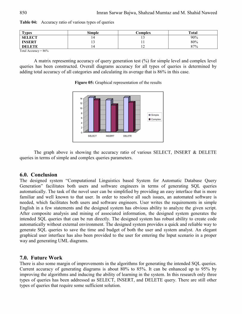
850 Imran Sarwar Bajwa, Shahzad Mumtaz and M. Shahid Naweed
Table 04: Accuracy ratio of various types of queries
Types Simple Complex Total SELECT 14 13 90% INSERT 13 11 80% DELETE 14 12 87%
Total Accuracy = 86%
A matrix representing accuracy of query generation test (%) for simple level and complex level queries has been constructed. Overall diagrams accuracy for all types of queries is determined by adding total accuracy of all categories and calculating its average that is 86% in this case.
Figure 05: Graphical representation of the results
0
2
4
6
8
10
12
14
SELECT INSERT DELETE
Simple
Complex
The graph above is showing the accuracy ratio of various SELECT, INSERT & DELETE queries in terms of simple and complex queries parameters. 6.0. Conclusion The designed system “Computational Linguistics based System for Automatic Database Query Generation” facilitates both users and software engineers in terms of generating SQL queries automatically. The task of the novel user can be simplified by providing an easy interface that is more familiar and well known to that user. In order to resolve all such issues, an automated software is needed, which facilitates both users and software engineers. User writes the requirements in simple English in a few statements and the designed system has obvious ability to analyze the given script. After composite analysis and mining of associated information, the designed system generates the intended SQL queries that can be run directly. The designed system has robust ability to create code automatically without external environment. The designed system provides a quick and reliable way to generate SQL queries to save the time and budget of both the user and system analyst. An elegant graphical user interface has also been provided to the user for entering the Input scenario in a proper way and generating UML diagrams. 7.0. Future Work There is also some margin of improvements in the algorithms for generating the intended SQL queries. Current accuracy of generating diagrams is about 80% to 85%. It can be enhanced up to 95% by improving the algorithms and inducing the ability of learning in the system. In this research only three types of queries has been addressed as SELECT, INSERT, and DELETE query. There are still other types of queries that require some sufficient solution.

Database Interfacing using Natural Language Processing 851
References [1] Allen,J. (1994) Natural Language Understanding. Benjamin- Cummings Publishing Company,
New York. [2] Biber, D., Conrad, S., & Reppen, R. (1998). Corpus Linguistics: Investigating Language
Structure and Use. Cambridge Univ. Press, Cambridge, U.K. [3] D. DeHaan, D. Toman, M. P. Consens, and T. Ozsu. (2003) A Comprehensive XQuery to SQL
Translation using Dynamic Interval Encoding. In SIGMOD. [4] C. A. Thompson, R. J. Mooney and L. R. Tang, Learning to parse natural language database
queries into logical form, in: Workshop on Automata Induction, Grammatical Inference and Language Acquisition (1997).
[5] Salton, G., & McGill, M. (1983). Introduction to Modern Information Retrieval. McGraw-Hill, New York.
[6] A. Rosenthal. D. Reiner, Extending the Algebraic Framework of Query Processing to Handle Outer joins, Proc. VLDB Singa- pore 1984. pp. 334-343.
[7] Fagan, J. L. (1989). The effectiveness of a non-syntactic approach to automatic phrase indexing for document retrieval. Journal of the American Society for Information Science, 40 (2), 115–132.
[8] J. M. Zelle and R. J. Mooney, Learning semantic grammars with constructive inductive logic programming, in: Proceedings of the 11th National Conference on Arti_cial Intelligence (AAAI Press/MIT Press, Washington, D.C., 1993), pp. 817ñ822.
[9] Kowalski, G. (1998). Information Retrieval Systems: Theory and Implementation. Kluwer, Boston.
[10] Krovetz, R., & Croft, W. B. (1992). Lexical ambiguity and information retrieval. ACM Transactions on Information Systems, 10, 115–141.
[11] Losee, R. M. (1988). Parameter estimation for probabilistic document retrieval models. Journal of the American Society for Information Science, 39(1), 8–16.
[12] Losee, R. M. (1996a). Learning syntactic rules and tags with genetic algorithms for information retrieval and filtering: An empirical basis for grammatical rules. Information Processing and Management, 32(2), 185–197.
[13] Manning, C. D., & Schutze, H. (1999). Foundations of Statistical Natural Language Processing. MIT Press, Cambridge, Mass.
[14] Partee, B. H., Meulen, A. t., &Wall, R. E. (1990). Mathematical Methods in Linguistics. Kluwer, Dordrecht, The Netherlands.
European Journal of Scientific Research ISSN 1450-216X Vol.20 No.4 (2008), pp.852-862 © EuroJournals Publishing, Inc. 2008 http://www.eurojournals.com/ejsr.htm
Role of Trade, External Debt, Labor Force and Education in
Economic Growth Empirical Evidence from Pakistan by using ARDL Approach
Arshad Hasan Muhammad Ali Jinnah University Islamabad
E-mail: [email protected]
Safdar Butt Dean faculty of Business Administration and Social Sciences
Mohammad Ali Jinnah University
Abstract
This paper examines the determinants of economic growth for Pakistan over a period of 1975-2005, using Autoregressive Regressive Distributed Lag (ARDL) approach to Cointegration. The relation ship between economic growth, trade, external debt, labor force and education has been discussed in long term and short term. And it is found that labor force and trade have significant impact on economic growth whereas external debt has no association with economic growth in long term or short term indicating that it has not been used efficiently and productively. An appropriate policy to educate and develop the human resources of the country coupled with export oriented policies can help in accelerating the process of economic development and growth and that in turn can have multidimensional positive effects on the economy and economic conditions of common man. Keywords: Pakistan, exports, human capital, causality, ARDL JEL Classification Codes: C12, C22
1. Introduction Pakistan’s economy has shown various ups and downs during last 30 years. This study explores the various factors that have impact on the long-term economic growth of the country. Some of the factors that affect the economic growth of a country include human capital, total trade external debt and education. An examination of the role of said factors in economic growth is more important for developing countries like Pakistan that are fighting against poverty.
Human capital has been considered as one of the primary engines of economic growth and development. Economic theory suggests that human capital is an important determinant of growth. Various theoretical models include human capital as a factor of production and consider the accumulation of human capital as an element of the growth process and empirical evidence for number of countries also confirms this relationship. Thus we can say that human resource development and its efficient management plays vital role in the economic growth of economy.
In emerging economies like Pakistan export can play a pivotal role in accelerating the process of economic growth. The export led hypothesis assumes that export expansion leads to better resource
Role of Trade, External Debt, Labor Force and Education in Economic Growth Empirical Evidence from Pakistan by using ARDL Approach 853
allocation and improves production efficiency. This is possible through technological development, new capital formation and employment creation which are pre requisites for accelerated economic growth. During last few decades, Pakistan has shifted from import substitution policy to export oriented policy. Economic reforms in the last five years have done much to boost Pakistan’s merchandise trade/GDP ratio. Evidence on relationship between trade and economic growth is mixed
Capital is an important factor of production. Capital inflows in the form of external debt can play a vital role in increasing the national output. However, excess use of such capital may have negative impact as it increases the debt servicing costs and can effect balance of payments. Empirical evidence suggests bidirectional causality between external debt and growth. Higher external debt lowers growth but at the same time low growth increases indebtedness. Higher debt operates through a strong negative effect on physical capital accumulation and on total factor productivity. Lower growth reduces revenues and primary surpluses. If these are not addressed and adjusted timely these can affect debt ratios. Reducing debt levels would therefore, contribute to growth by boosting both capital accumulation and productivity growth.
This study analyzes the relationship between economic growth, human capital, trade and external debt and education for the period 1995-2005. The paper is organized as follows.
The section II provides an overview of the existing literature about the relationship between economic growth, exports, human capital external debt and education. The data employed and methodology adopted has been explained in section III. Empirical results have been discussed in section IV. Section V deals with conclusion and policy implications 2. Literature Review 2.1. Human Capital and Economic Growth
Lucas (1993) argues that accumulation of human capital serves as an engine of growth. Human capital accumulation takes place in schools, in research organizations, and in the course of producing goods and engaging in trade.He investigates the reasons of diversity in the quality of life among nations and finds that major source of difference is the dissimilarity in human capital. Mankiw (1992) further extends the theory and considers human capital as an additional accumulate able factor. He provides evidence that changes in human capital ultimately translates into significant changes of growth rates.
Relationship between economic growth and human capital has been examined extensively. Many theoretical models of economic growth exists which include Nelson and Phelps (1966), Lucas (1988), Becker, Murphy, and Tamura (1990), Rebelo (1992), and Mulligan and Sala-i-Martin (1992). Many empirical researchers which include Romer(1990), Barro(1991),Benhabib and Spiegel(1994) provide evidence that economic growth and schooling are correlated across countries and time.
Studies that examine the relationship between economic growth and human capital accumulation are divided into two broader categories. First group of studies uses growth accounting framework. The growth accounting framework assumes that education, increases the human capital stock of individuals that improves their productivity and ultimately contributes to growth. This group includes the studies of Baumol(1986), Barro(1991), Barro and Lee(1993). Other group of studies employs endogenous growth model. The endogenous growth models assume that human capital creates new ideas which is transformed into scientific knowledge and ultimately leads to accelerate the process of economic growth. This group includes Lucas (1988), Romer(1990), Grossman (1991).
Barro(1991), Barro and Lee(1993),Benhabib and Spiegel(1994)provide evidence that human capital accumulation promotes economic growth). Bils and Klenow (2000) take up the matter differently and find that levels of schooling are positively correlated with growth rates. But they find that direction of relation is debatable. Here question arises whether increased schooling results in accelerated economic growth or accelerated economic growth leads to attainment of higher schooling due to better allocation of resources for education in the country. However, relatively few studies have
854 Arshad Hasan and Safdar Butt
tested for causality between human capital formation and economic growth. Studies which test for causality between human capital and growth within a bivariate framework are De Meulemeester and Rochat (1995), In and Doucouliagos (1997) and Asteriou and Agiomirgianakis (2001). 2.2. Trade and Economic Growth
Relationship between trade and economic growth has been examined extensively. There are number of studies that empirically investigate the relationship between exports and growth. These studies either use correlation analysis or employ causality techniques. The empirical evidence on the export growth nexus is mixed with no clear consensus. Ahmad (2001) reviews approximately 40 studies conducted during 1970-1990 and finds that empirical support for the export led growth in developing and developed countries is considerably weaker in more recent studies. Results for studies that use cointegration and causality analysis are significantly different from those studies which are based on correlation analysis. Summers (1997) examines the relationship between total trade and growth for Australian and Canadian market and finds that imports and exports trade play different roles on economic growth. Summers finds that import trade has a significance role in Canada. However no evidence of in support of export led growth is found for Australian economy. Strydom (2003) studies the role of foreign sector in economy and finds that international trade does not play a significant role in economic growth .One possible reason for this ambiguity is the lack of understanding of the diffusion system that links trade with economic growth. The evidence shows that the channels through which trade generates growth have asymmetric growth effects. Therefore economic policies should be structured to eliminate the impeding effects for such channels and to augment the efficiency of less efficient mechanism.
Human capital accumulation increases the quality of labor, which in turn, enhances the productivity of the workforce and stimulates further exports and economic growth (Chuang 2000). Hanson and Harrison (1995), Stokey(1996) and many other Empirical studies suggest that trade promotes human capital accumulation and vice-versa. Support for said argument is wide spread covering range of countries and time periods. 2.3. External Debt and Economic Growth
External debt serves as catalyst to mobilize other factors of production. In many countries, external debt has been used as main source of capital investment for development of the physical infrastructure. However, there has been a concern regarding the proper utilization of external debt in poverty alleviation and overall economic growth of the country.
The relationship between external debt and economic growth has been examined extensively in recent years. These studies have largely focused on the harmful effects of a country’s “debt overhang”. It is meant that debt is accumulated to such a high level that becomes a threat for the borrower country and it faces problems in servicing the debts. The empirical findings suggest that debt overhang depresses growth by increasing investors’ uncertainty about actions the government might take to meet its onerous debt-servicing obligations. Debt overhang may also affect the efforts of the government to carry out structural and fiscal reforms which are necessary to accelerate the economic growth process of the country. Governments also feel pressures to retire foreign debts. Pakistan’s external debt situation of the 1990s is consistent with the findings of the recent literature on the relationship between debt and economic growth. If take an overview of the last decade we find that large current account deficit (almost 5.0percent of GDP) for an extended period of one decade, the irresponsible use of borrowed funds, mounting real cost of borrowing and stagnant exports have contributed significantly in quick accumulation of external debt.
A number of studies have examined the relationship between external debt and economic growth. The majority of these studies have found that debt variables are significantly and negatively correlated with growth. Maureen (2001) analyses the magnitude and structure of Kenya's external debt and examines its impact on economic growth and private investment using time series data for the
Role of Trade, External Debt, Labor Force and Education in Economic Growth Empirical Evidence from Pakistan by using ARDL Approach 855
period 1970- 1995. The empirical results show that external debt accumulation has a negative impact on economic growth of Kenya. Karagol (1999) examines the relationship between economic growth, external debt service and capital inflow using the time series data for Turkey and employing simultaneous equations. The result suggests that the rise in the debt-servicing ratio adversely affects economic growth, whereas the decrease in the rate of growth reduces the ability of an economy to service its debt. This study further provides that the direct impact of external debt on the economic growth is negative. However favorable indirect effects of it exceed the direct effects. Chowdhury (1994) investigates the direct, indirect of the external debt on economic growth of seven countries by using panel data for the period of 1970-1988. These countries include Bangladesh, Indonesia, Malaysia, Philippines, South Korea, Sri Lanka and Thailand. Results suggest that the external debt of developing countries is not a primary cause of economic slow down. Schclarek (2004) examines the probability of existence of both linear and nonlinear relationship between debt and economic growth for developing and industrial countries. Evidence here is mixed. In case of developing countries, a significant negative relationship has been observed between external debt and economic growth. However, no such relationship has been observed in case of industrial countries.
The literature survey shows that a number of studies have examined the role of external debt, labor force and trade in economic growth separately. But there is no single study examining the role of these variables in the economy in an integrated way. In this regard, this study attempts to bridge this gap. 3. Data Description and Methodology 3.1. Data Description and Definition of Variables
This study examines the relationship between economic growth, trade, external debt, human capital and education. Data on all variables is taken from various publications of State Bank of Pakistan, Bureau of Statistics, Economic Survey of Pakistan and Lee and Barro’s database on human capital measures. The study uses annual data that cover the period from 1975 -2005. 3.2. Dependent variable
The economic growth is used as the dependent variable in the model. Gross domestic product (GDP) is employed as the proxy of the economic growth 3.3. Independent variables
The independent variables are Education, Total Trade, External Debt and Labor Force. Education A review empirical work on the relationship between human capital and growth reveals that various proxies have been used to measure the human capital stock. Alternative proxies for human capital includes school enrolment ratios, adult literacy rates, levels of education attainment and average years of schooling, monetary value of human capital stock and international test scores of students. These are very diversified but all have limitations in one way or other.
School enrolment ratios, adult literacy rates are extensively used in growth regressions due to their easy availability and broad coverage. Adult literacy rates ignore most of the investments made in human capital as they do not include qualifications obtained above the basic levels of education so it seems to be a poor measure of human capital available for current production. Enrolment ratios are flow variables, and the children currently enrolled in schools are not yet part of the labor force. Therefore, enrolment ratios do not accurately represent changes in human capital stock. Levels of education and average years of schooling are most popular and commonly used measures today. This
856 Arshad Hasan and Safdar Butt
study uses average years of schooling of the working age population as a proxy for Education .It is hypothesized that there exists a positive relationship between education and economic growth. Total Trade Trade plays an important role in increasing the production of goods and services. Total trade is the sum of total exports and imports. All data has been converted into Pakistani rupees and it is transformed at constant prices of 2000 to adjust the impact of exchange rate variations. It is hypothesized that there exists a positive relationship between trade and economic growth. External Debt External debt is one of the major sources of financing the development programs. These programs generally focus on infrastructure development that is necessary to lay down the foundations of sustainable economic growth. It is hypothesized that there exists a positive relationship between external debt and economic growth. For this study External debt has been translated into Pakistani rupees at constant prices of 2000 and then logarithm of External debt is taken to construct the variable. It is hypothesized that there exists a negative relationship between external debt and economic growth. Labor Force Labor force is directly involved in the production process and large labor force can help to enhance production of goods and services. For purpose of this study Labor force of the age between 15 and 64 has been taken from Economic Survey of Pakistan. It is hypothesized that there exists a positive relationship between labor force and economic growth. 3.4. Methodology
To examine the impact of human capital, trade, external debt and education on economic growth following model has been tested
Ln GDPt = β0+ β1 lnTT t+ β2 lnLF t + β3 lnTD t + β4 Edu t+µt (1) Where
GDP= gross domestic product (in constant terms for year 2000) TT = total trade LF= labor force in the age range of 15-64 TD = total debt at constant Rate Education = average year of schooling
Existence of the long run equilibrium relationship among chronological variables can be investigated by using several methods. The most widely used methods include Engle and Granger (1987) test, fully modified OLS procedure of Phillips and Hansen’s (1990), maximum likelihood based Johansen (1988, 1991) and Johansen-Juselius (1990) tests. All these methods require that the variables in the system are integrated of order one I (1). Futher, these methods are considered as weak as these methods do not provide robust results for small samples or structural breaks. Due to these problems, a newly developed autoregressive distributed lag (ARDL) approach to cointegration has become popular in recent years.
The ARDL modeling approach was originally introduced by Pesaran and Shin (1999) and further extended by Pesaran (2001). This approach has numerous econometric advantages in comparison to other Cointegration methods. One major advantage of ARDL approach is that it can be applied irrespective of degree of integration. Secondly, ARDL approach provides robust results in small sample sizes and estimates of the long-run coefficients are well consistent in small sample sizes( Pesaran and Shin 1999).
Furthermore, a dynamic error correction model (ECM) can be derived from ARDL that integrates the short-run dynamic with the long-run equilibrium without losing long run information. In view of the above advantages, we use ARDL approach for cointegration analysis and the resulting ECM.
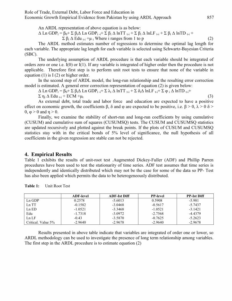
Role of Trade, External Debt, Labor Force and Education in Economic Growth Empirical Evidence from Pakistan by using ARDL Approach 857
An ARDL representation of above equation is as below: ∆ Ln GDPt = β0+ Σ βi∆ Ln GDPt -i+ Σ βi ∆ lnTT t-i + Σ βi ∆ lnLF t-i + Σ βi ∆ lnTD t-i +
Σ βi ∆ Edu t-i +µ t Where i ranges from 1 to p (2) The ARDL method estimates number of regressions to determine the optimal lag length for
each variable. The appropriate lag length for each variable is selected using Schwartz-Bayesian Criteria (SBC).
The underlying assumption of ARDL procedure is that each variable should be integrated of orders zero or one i.e. I(0) or I(1). If any variable is integrated of higher order then the procedure is not applicable. Therefore first step is to perform unit root tests to ensure that none of the variable in equation (1) is I (2) or higher order.
In the second step of ARDL model, the long-run relationship and the resulting error correction model is estimated. A general error correction representation of equation (2) is given below:
∆ Ln GDPt = β0+ Σ βi∆ Ln GDPt -i+ Σ λi ∆ lnTT t-i + Σ δi∆ lnLF t-i+ Σ φ i ∆ lnTD t-i+ Σ ηi ∆ Edu t-i + ECM +µt (3) As external debt, total trade and labor force and education are expected to have a positive
effect on economic growth, the coefficients β, δ and φ are expected to be positive, i.e. β > 0, λ > 0 δ > 0, φ > 0 and η > 0.
Finally, we examine the stability of short-run and long-run coefficients by using cumulative (CUSUM) and cumulative sum of squares (CUSUMSQ) tests. The CUSUM and CUSUMSQ statistics are updated recursively and plotted against the break points. If the plots of CUSUM and CUSUMSQ statistics stay with in the critical bonds of 5% level of significance, the null hypothesis of all coefficients in the given regression are stable can not be rejected. 4. Empirical Results Table 1 exhibits the results of unit-root test .Augmented Dickey-Fuller (ADF) and Phillip Parren procedures have been used to test the stationarity of time series. ADF test assumes that time series is independently and identically distributed which may not be the case for some of the data so PP- Test has also been applied which permits the data to be heterogeneously distributed. Table 1: Unit Root Test ADF-level ADF-Ist Diff PP-level PP-Ist Diff Ln GDP 0.2578 -5.6013 0.5908 -5.981 Ln TT -0.1582 -3.0468 -0.5617 -5.7437 Ln ED -1.0521 -3.3468 -1.0521 -3.1421 Edu -1.7318 -3.0972 -2.7568 -4.4379 Ln LF -0.43 -3.5870 -0.7625 -5.2623 Critical. Value 5% -2.9640 -2.9678 -2.9640 -2.9678
Results presented in above table indicate that variables are integrated of order one or lower, so
ARDL methodology can be used to investigate the presence of long term relationship among variables. The first step in the ARDL procedure is to estimate equation (2)
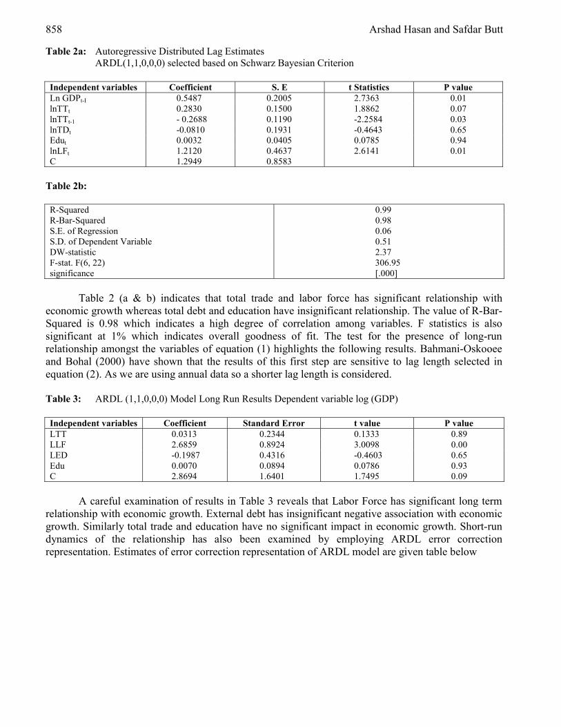
858 Arshad Hasan and Safdar Butt
Table 2a: Autoregressive Distributed Lag Estimates ARDL(1,1,0,0,0) selected based on Schwarz Bayesian Criterion
Independent variables Coefficient S. E t Statistics P value Ln GDPt-I 0.5487 0.2005 2.7363 0.01 lnTTt 0.2830 0.1500 1.8862 0.07 lnTTt-1 - 0.2688 0.1190 -2.2584 0.03 lnTDt -0.0810 0.1931 -0.4643 0.65 Edut 0.0032 0.0405 0.0785 0.94 lnLFt 1.2120 0.4637 2.6141 0.01 C 1.2949 0.8583
Table 2b: R-Squared 0.99 R-Bar-Squared 0.98 S.E. of Regression 0.06 S.D. of Dependent Variable 0.51 DW-statistic 2.37 F-stat. F(6, 22) 306.95 significance [.000]
Table 2 (a & b) indicates that total trade and labor force has significant relationship with
economic growth whereas total debt and education have insignificant relationship. The value of R-Bar-Squared is 0.98 which indicates a high degree of correlation among variables. F statistics is also significant at 1% which indicates overall goodness of fit. The test for the presence of long-run relationship amongst the variables of equation (1) highlights the following results. Bahmani-Oskooee and Bohal (2000) have shown that the results of this first step are sensitive to lag length selected in equation (2). As we are using annual data so a shorter lag length is considered. Table 3: ARDL (1,1,0,0,0) Model Long Run Results Dependent variable log (GDP) Independent variables Coefficient Standard Error t value P value LTT 0.0313 0.2344 0.1333 0.89 LLF 2.6859 0.8924 3.0098 0.00 LED -0.1987 0.4316 -0.4603 0.65 Edu 0.0070 0.0894 0.0786 0.93 C 2.8694 1.6401 1.7495 0.09
A careful examination of results in Table 3 reveals that Labor Force has significant long term
relationship with economic growth. External debt has insignificant negative association with economic growth. Similarly total trade and education have no significant impact in economic growth. Short-run dynamics of the relationship has also been examined by employing ARDL error correction representation. Estimates of error correction representation of ARDL model are given table below
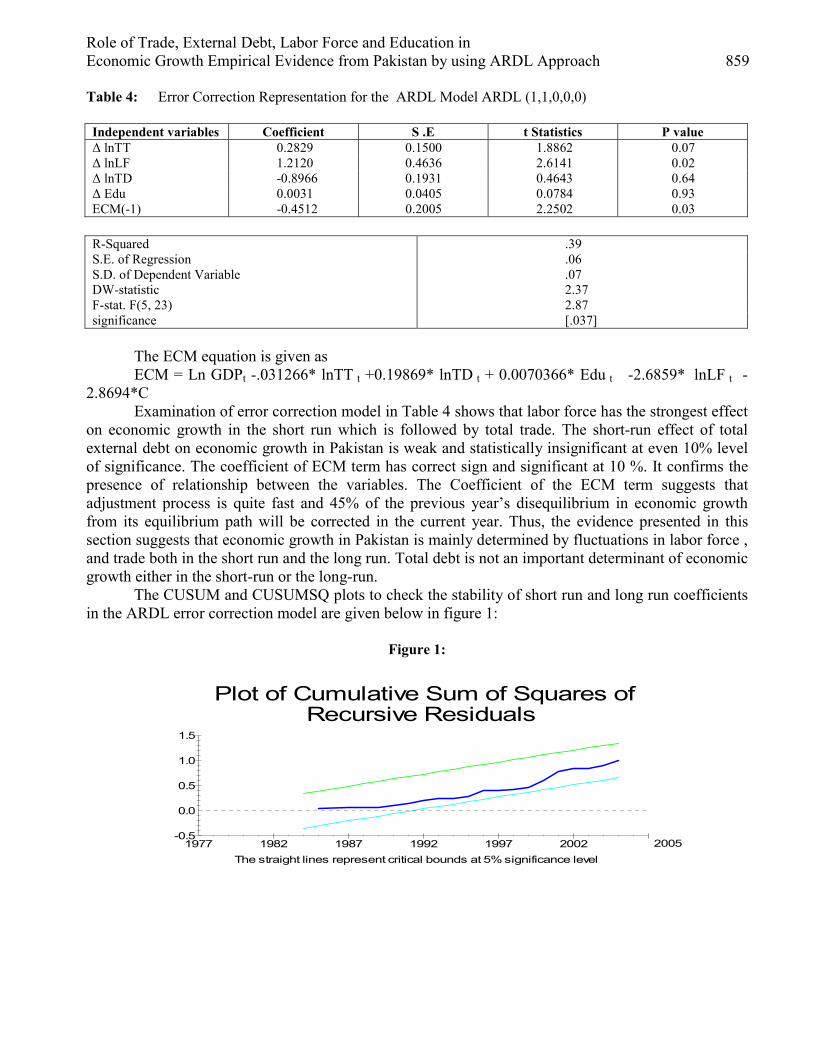
Role of Trade, External Debt, Labor Force and Education in Economic Growth Empirical Evidence from Pakistan by using ARDL Approach 859
Table 4: Error Correction Representation for the ARDL Model ARDL (1,1,0,0,0) Independent variables Coefficient S .E t Statistics P value ∆ lnTT 0.2829 0.1500 1.8862 0.07 ∆ lnLF 1.2120 0.4636 2.6141 0.02 ∆ lnTD -0.8966 0.1931 0.4643 0.64 ∆ Edu 0.0031 0.0405 0.0784 0.93 ECM(-1) -0.4512 0.2005 2.2502 0.03
R-Squared .39 S.E. of Regression .06 S.D. of Dependent Variable .07 DW-statistic 2.37 F-stat. F(5, 23) 2.87 significance [.037]
The ECM equation is given as ECM = Ln GDPt -.031266* lnTT t +0.19869* lnTD t + 0.0070366* Edu t -2.6859* lnLF t -
2.8694*C Examination of error correction model in Table 4 shows that labor force has the strongest effect
on economic growth in the short run which is followed by total trade. The short-run effect of total external debt on economic growth in Pakistan is weak and statistically insignificant at even 10% level of significance. The coefficient of ECM term has correct sign and significant at 10 %. It confirms the presence of relationship between the variables. The Coefficient of the ECM term suggests that adjustment process is quite fast and 45% of the previous year’s disequilibrium in economic growth from its equilibrium path will be corrected in the current year. Thus, the evidence presented in this section suggests that economic growth in Pakistan is mainly determined by fluctuations in labor force , and trade both in the short run and the long run. Total debt is not an important determinant of economic growth either in the short-run or the long-run.
The CUSUM and CUSUMSQ plots to check the stability of short run and long run coefficients in the ARDL error correction model are given below in figure 1:
Figure 1:
Plot of Cumulative Sum of Squares ofRecursive Residuals
The straight lines represent critical bounds at 5% significance level
-0.5
0.0
0.5
1.0
1.5
1977 1982 1987 1992 1997 2002 2005
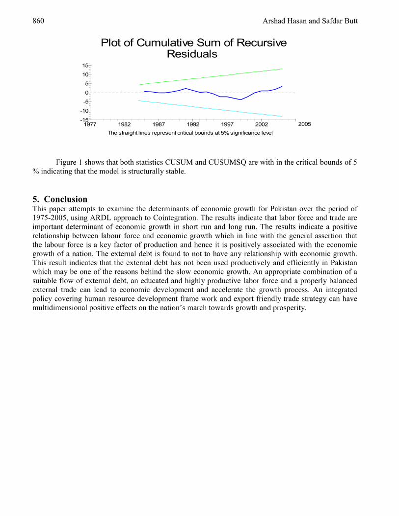
860 Arshad Hasan and Safdar Butt
Figure 1 shows that both statistics CUSUM and CUSUMSQ are with in the critical bounds of 5 % indicating that the model is structurally stable. 5. Conclusion This paper attempts to examine the determinants of economic growth for Pakistan over the period of 1975-2005, using ARDL approach to Cointegration. The results indicate that labor force and trade are important determinant of economic growth in short run and long run. The results indicate a positive relationship between labour force and economic growth which in line with the general assertion that the labour force is a key factor of production and hence it is positively associated with the economic growth of a nation. The external debt is found to not to have any relationship with economic growth. This result indicates that the external debt has not been used productively and efficiently in Pakistan which may be one of the reasons behind the slow economic growth. An appropriate combination of a suitable flow of external debt, an educated and highly productive labor force and a properly balanced external trade can lead to economic development and accelerate the growth process. An integrated policy covering human resource development frame work and export friendly trade strategy can have multidimensional positive effects on the nation’s march towards growth and prosperity.
Plot of Cumulative Sum of RecursiveResiduals
The straight lines represent critical bounds at 5% significance level
-5
-10
-15
0
5
10
15
1977 1982 1987 1992 1997 2002 2005

Role of Trade, External Debt, Labor Force and Education in Economic Growth Empirical Evidence from Pakistan by using ARDL Approach 861
References [1] Bahmani-Oskooee, M. and Bohl, M. T., “German monetary unification and the stability of
German M3 money demand function” Economic Letters, Vol.66, 2000, pp.203-208. [2] Engle, R. and Granger, C., “Cointegration and error and testing”, Econometrica, 55, 1987,
pp.251-276. [3] Johansen, S., “Statistical analysis of cointegrating vectors”, Journal of Economic Dynamics and
Control, Vol.12, 1988, pp.231-254 [4] Johansen, S. and Juselius, K., “Maximum likelihood estimation and inference on cointegration
–with application to the demand for money” Oxford Bulletin of Economics and Statistics, Vol. 52, 1990, pp.169-210.
[5] Peseran, M. H. and Shin, Y., An Autoregressive Distributed Lag Modelling Approach to Cointegration Analysis. Chapter 11 in Econometrics and Economic Theory in 20th Century: The Ragnar Frisch Centennial Symposium, Strom, S. (ed.). (Cambridge University Press: Cambridge, 1999)
[6] Pesaran, M. H. and B. Pesaran, B., Microfit 4.0 Interactive Econometric Analysis (Oxford University Press, Oxford, 1997).
[7] Chowdhury, Khorshed (1994). "A Structural Analysis of External Debt and Economic Growth: Some Evidence from Selected Countries in Asia and the Pacific." Applied Economics 26: 1121-1131.
[8] Kalima, Barbara (2002). "Gender and Debt". African Forum and Network on Debt & Development, pp: 6-7.
[9] Maureen Were (2001). "The Impact of External Debt on Economic Growth and Private Investment in Kenya." Kenya Institute for Public Policy Research and Analysis, pp: 28-30
[10] Shrestha, Min B. and Khorshed Chowdhury (2005). "A Sequential Procedure for Testing Unit Roots in the Presence of Structural Break in Time Series Data". International Journal of Applied Econometrics and Quantitative Studies, 2, pp: 1-15.
[11] Strydom, P.D.F. (2003). International trade and economic growth in South Africa, The Economic Society of South Africa.
[12] Summers, Peter M. (1997). "Trade and Growth in Settle Economies: Australian and Canadian Comparisons", Melbourne Institute Working Papers 9/97 pp.6
[13] Barro, R., (1991), “Economic Growth in a Cross Section of Countries,” Quarterly Journal of Economics, 106, 407-33.
[14] Barro, R. and J.-W. Lee, (1993), “International Comparisons of Educational Attainment,” Journal of monetary Economics, 32, 363-94.
[15] Ramesh Paudel and Min B Shrestha (2006),” The Role of External Debt, Total Trade and Labour Force in Economic Growth: The case of Nepal” ,The Business Review, Cambridge; Summer 2006; 5, 2; ABI/INFORM Global pg. 130
[16] De Meulemeester, J. L. and D. Rochat, (1995), “A Causality Analysis of the Link Between Higher Education and Development,” Economics of Education Review, 14, 351-61
[17] Chuang, (2000), " Human Capital, Exports, and Economic Growth: A Causality Analysis for Taiwan, 1952-1995" . Review of International Economics, Vol. 8, pp. 712-720, November
[18] In, F. and C. Doucouliagos, (1997), “Human Capital Formation and US Economic Growth: A Causality Analysis,” Applied Economics Letters, 4, 329-31.
[19] Lucas, R E(1988). "On the Mechanics of Development Planning." Journal of Monetary Economics, 22. pp. 3-42.
[20] Romer, P. (1990), “Human Capital and Growth: Theory and Evidence,” Carnegie-Rochester Conference Series on Public Policy, 32, 251-285.
[21] Grossman. G M. and E Helpman (1991), “Innovation and growth in global ~Cam briddge, Massachusetts M.I.T. Press.

862 Arshad Hasan and Safdar Butt
[22] Benhabib, J. and M. Spiegel, (1994), “The Role of Human Capital in Economic Development: Evidence from Cross-Country Data,” Journal of Monetary Economics, 34, 143-73.
[23] Asteriou, D. and G. M. Agiomirgianakis, (2001), “Human Capital and Economic Growth: Time Series Evidence from Greece,” Journal of Policy Modeling, 23, 481-89.
[24] Barro, R., (1991), “Economic Growth in a Cross Section of Countries,” Quarterly Journal of Economics, 106, 407-33.
[25] Barro, R. and J.-W. Lee, (1993), “International Comparisons of Educational Attainment,” Journal of monetary Economics, 32, 363-94.
[26] Pesaran, M. H., Y. Shin, and R. Smith (2001). “Bounds Testing Approaches to the Analysis of Level Relationships,” Journal of Applied Econometrics, 16(3), 289
[27] Barro, R. J. and X. Sala-i-Martin (1999), Economic Growth. New York: McGraw-Hill. [28] Pesaran, M. H. and B. Pesaran.(1997),”Working with Microfit 4.0: Interactive Econometric
Analysis”, Oxford: Oxford University Press. [29] Ahmad, J. (2001), “Causality Between Exports and Economic Growth: What Do the
Econometric Studies Tell Us?” , Pacific Economic Review, 6(1), 147-167. [30] Bils, M. and P. Klenow. (2000), “Does Schooling Cause Growth?” American Economic
Review, 90(5), 1160-1183.

European Journal of Scientific Research ISSN 1450-216X Vol.20 No.4 (2008), pp.863-870 © EuroJournals Publishing, Inc. 2008 http://www.eurojournals.com/ejsr.htm
Development of Mechanical Prosthetic Hand System for BCI
Application
N. A Abu Osman Department of Biomedical Engineering, Faculty of Engineering
University of Malaya, 50603, Kuala Lumpur, Malaysia
S. Yahud Department of Biomedical Engineering, Faculty of Engineering
University of Malaya, 50603, Kuala Lumpur, Malaysia
S. Y Goh Department of Biomedical Engineering, Faculty of Engineering
University of Malaya, 50603, Kuala Lumpur, Malaysia
Abstract
The study is to develop a prosthetic hand that can be controlled by Brain-Computer Interface (BCI). The proposed prosthetic hand consists of palm and 5 fingers. The hand was designed to perform the 4 predetermined essential tasks in BCI applications; cylindrical grasp, key pinch, pulp to pulp pinch and tripod pinch. The phalanges of the finger was modeled as three link open chain joined at the metacarpal joint (MCP), proximal joint (PIP) and distal joint (DIP). Each segment denote as phalanx was made from two parallel aluminum plates and connected to the other segment using a bolted spacer acting as hinge joint. Length of each segment was made such that it will form an equiangular motion path during trajectory. Each joint is actuated by its individual actuator. Two mechanisms were proposed in this study. The first mechanism is the tendon drive; used terelyne string to pull each segment to flexion. The second mechanism is a spring return; a stored resistive force in torsion spring will kick the segment to its initial position. The hand was equipped with potentiometers and pressure sensors for control purposes. The prototype was tested with BCI system, in order to meet its initial objective and additional tests were carried out to evaluate its performance. An experiment to test the performance of the prosthetic hand was carried out successfully. Strength of each tendon was measured using a proof ring method and motion images were captured using video camera and analyzed using Peak Motus Performance 2000 Motion Analysis software.
1.0. Introduction Brain-Computer interface
A brain-computer interface (BCI) is a communication system in which messages or commands convey from an individual to external device without passing through a brain's normal output pathways of peripheral nerves and muscles. A BCI use the recorded electroencephalogram (EEG) rhythms from the electrodes on scalp and translated to the external device. The BCI application is useful for people with severe motor disabilities and in worst case for a completely paralyzed or “locked-in” patient that unable to communicate by any way. BCI application is wide and can be varied depending on the need
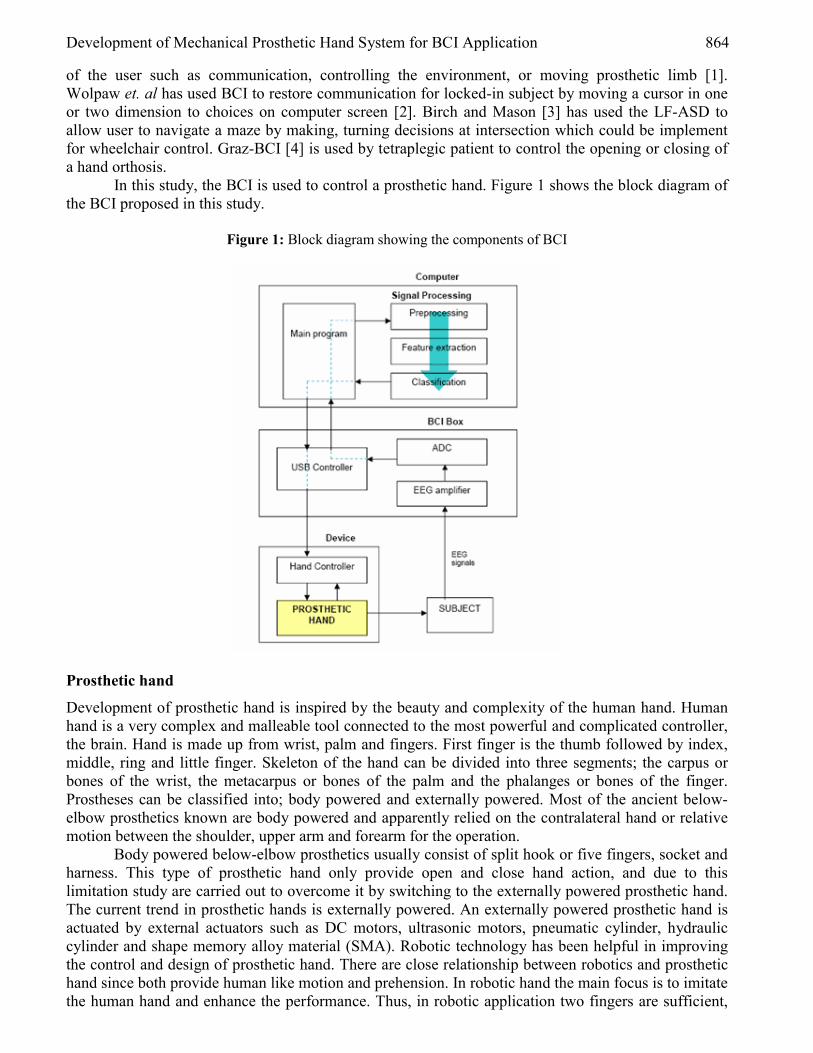
Development of Mechanical Prosthetic Hand System for BCI Application 864
of the user such as communication, controlling the environment, or moving prosthetic limb [1]. Wolpaw et. al has used BCI to restore communication for locked-in subject by moving a cursor in one or two dimension to choices on computer screen [2]. Birch and Mason [3] has used the LF-ASD to allow user to navigate a maze by making, turning decisions at intersection which could be implement for wheelchair control. Graz-BCI [4] is used by tetraplegic patient to control the opening or closing of a hand orthosis.
In this study, the BCI is used to control a prosthetic hand. Figure 1 shows the block diagram of the BCI proposed in this study.
Figure 1: Block diagram showing the components of BCI
Prosthetic hand
Development of prosthetic hand is inspired by the beauty and complexity of the human hand. Human hand is a very complex and malleable tool connected to the most powerful and complicated controller, the brain. Hand is made up from wrist, palm and fingers. First finger is the thumb followed by index, middle, ring and little finger. Skeleton of the hand can be divided into three segments; the carpus or bones of the wrist, the metacarpus or bones of the palm and the phalanges or bones of the finger. Prostheses can be classified into; body powered and externally powered. Most of the ancient below-elbow prosthetics known are body powered and apparently relied on the contralateral hand or relative motion between the shoulder, upper arm and forearm for the operation.
Body powered below-elbow prosthetics usually consist of split hook or five fingers, socket and harness. This type of prosthetic hand only provide open and close hand action, and due to this limitation study are carried out to overcome it by switching to the externally powered prosthetic hand. The current trend in prosthetic hands is externally powered. An externally powered prosthetic hand is actuated by external actuators such as DC motors, ultrasonic motors, pneumatic cylinder, hydraulic cylinder and shape memory alloy material (SMA). Robotic technology has been helpful in improving the control and design of prosthetic hand. There are close relationship between robotics and prosthetic hand since both provide human like motion and prehension. In robotic hand the main focus is to imitate the human hand and enhance the performance. Thus, in robotic application two fingers are sufficient,

865 N. A Abu Osman, S. Yahud and S. Y Goh
however three fingers are needed to perform dexterous tasks in an unstructured environment and to achieve full grasp of two-dimensional object [5]. Whereas, prosthetic hands are inspired by the need to replace the function of the human hand and try the best to resemble the human hand both functionally and structurally. In general prosthetic hands have benefited from the development of the robotic technologies. Brain-computer interface (BCI) project developed by University of Malaya is a project consists of signal processing part, BCI box and the device, as shown in figure 1. The device is composed of prosthetic hand and fuzzy controller. The objective of the study is to develop a prosthetic hand that able to perform the four basic tasks required by human hand: cylindrical grasps, key pinch, pulp to pulp pinch and tripod pinch. 2.0. Methodology In this study the primary concern is to develop a prosthetic hand that able to perform the four essential tasks using a BCI system. In order for the hand to perform the four tasks, the hand should possess the maximum number of the DOFs. As a result, the proposed design should yield a total of 16 DOFs with each finger has 3 DOFs and thumb has 4 DOFs. The design of the finger has the following characteristics; (i) each finger has a total of three joints with three DOFs, (ii) thumb has similarly three joints but with four DOFs, (iii) each DOF is actuated by one actuator, (iv) each joint has installed a torsion spring within it for return mechanism, and (v) each joint is equipped with potentiometer for control. For every DOF of movements, it is driven by its individual actuator, thus the hand used up to 16 units of actuator. Actuator used in this design is DC micromotors type 1331 with gearhead reduction series 14/1 manufactured by Faulhaber Group. The actuator is then connected to its respective segment using a terelyne string. The string will pulled the segment as the actuator rotates, the angle and speed of the flexion is depending on the output of the actuator. Flexion of each segment is accomplished when the string being pulled by the actuator and reset to its original position when string releases. The reset mechanism is, attain with the used of torsion spring at the joint. The stored resistive force on the torsion spring will reset segment to its original position. The string will act as a flexor digitorum profundus tendon of the human hand. The basic unit of the prosthetic hand is the prosthetic finger. Each prosthetic finger is said to maintain the same anatomical structure and dimensional proportion, regardless of their size. The three phalanx; distal, middle and proximal phalanges are denoted as L3, L2 and L1 accordingly as shown in figure 2 and connected to form a finger as shown in figure 3.
Figure 2: Different size and shape of phalanx

Development of Mechanical Prosthetic Hand System for BCI Application 866
Figure 3: Prosthetic finger
Each phalanx is made from 2-parallel aluminum plate of 1.5mm thickness and join using a brass spacer bolted with 2mm diameter stainless steel screw. DC motors with the combination of reduced gear heads are used to actuate finger segments. Process of determining the length of the phalanx acquired the implementation of the Fibonacci sequence. Fibonacci sequence in application to the human hand stated that; the difference between the length of the next phalanx and the sum length of the two prior phalanges must equal to zero. The sum of the distal phalanx and the middle phalanx should be equal to the length of the proximal phalanx. However, Park et al [6] in his work has showed that the bone lengths of the finger does not follow the Fibonacci relationship but the motion paths of the digits still form an equiangular spiral path. Therefore to achieve the equiangular spiral motion path the respective length that representing each segment should include the absolute bone length and functional length (radius of the joint). Length of each segment was referred to author’s hand herself and using the Hamilton’s ratio [7] to verify that the chosen length is sufficient to form an equiangular spiral motion.
All the fabrication and machining process was done in the mechanical workshop in the Department of Mechanical Engineering, University of Malaya, Malaysia. The precise machining was carried out using a CNC (computer numerical control) wire EDM (electrical discharge machining) machine Sodick, available in the Department of Manufacturing and Design, University of Malaya, Malaysia. 3.0. Result A prototype of prosthetic hand was successfully fabricated and tested for functionality, performance and strength. Figure 4 shows the flow diagram of a BCI system to control prosthetic hand developed by Biomedical Engineering BCI group, University of Malaya. A fuzzy controller is used to control the prosthetic hand. Input for controller is fed from the BCI box. EEG signals acquired from subject is amplified and converted to digital signal. The signal is further process and classified before send to fuzzy controller.
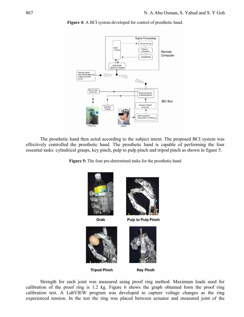
867 N. A Abu Osman, S. Yahud and S. Y Goh
Figure 4: A BCI system developed for control of prosthetic hand.
The prosthetic hand then acted according to the subject intent. The proposed BCI system was effectively controlled the prosthetic hand. The prosthetic hand is capable of performing the four essential tasks: cylindrical grasps, key pinch, pulp to pulp pinch and tripod pinch as shown in figure 5.
Figure 5: The four pre-determined tasks for the prosthetic hand
Strength for each joint was measured using proof ring method. Maximum loads used for calibration of the proof ring is 1.2 kg. Figure 6 shows the graph obtained form the proof ring calibration test. A LabVIEW program was developed to capture voltage changes as the ring experienced tension. In the test the ring was placed between actuator and measured joint of the
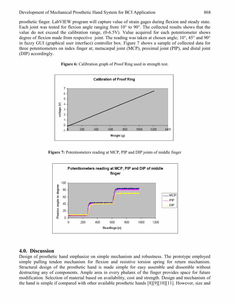
Development of Mechanical Prosthetic Hand System for BCI Application 868
prosthetic finger. LabVIEW program will capture value of strain gages during flexion and steady state. Each joint was tested for flexion angle ranging from 10° to 90°. The collected results shows that the value do not exceed the calibration range, (0-6.5V). Value acquired for each potentiometer shows degree of flexion made from respective joint. The reading was taken at chosen angle; 10°, 45° and 90° in fuzzy GUI (graphical user interface) controller box. Figure 7 shows a sample of collected data for three potentiometers on index finger at; metacarpal joint (MCP), proximal joint (PIP), and distal joint (DIP) accordingly.
Figure 6: Calibration graph of Proof Ring used in strength test.
Figure 7: Potentiometers reading at MCP, PIP and DIP joints of middle finger
4.0. Discussion Design of prosthetic hand emphasize on simple mechanism and robustness. The prototype employed simple pulling tendon mechanism for flexion and resistive torsion spring for return mechanism. Structural design of the prosthetic hand is made simple for easy assemble and dissemble without destructing any of components. Ample area in every phalanx of the finger provides space for future modification. Selection of material based on availability, cost and strength. Design and mechanism of the hand is simple if compared with other available prosthetic hands [8][9][10][11]. However, size and

869 N. A Abu Osman, S. Yahud and S. Y Goh
weight of the prosthetic hand could be reduced and skin could be added into the design to give more humanlike impression.
Functional strength on each joint is depending on the tendon’s material. Terelyne string is used as tendon and able to withstand a maximum functional weight of 45 kg. Therefore, the prosthetic hand is capable of handling functional weight more than required by human hand [12]. The path of fingertip trajectory for each prosthetic finger is similar to Guo’s trajectory [13]. Maximum flexion angles for each joint are varied but approaching the value suggested by Thakor et. al [14]. The prosthetic hand is able to pose the four desired tasks without reaching a maximum angle of each joint. The four tasks focused in the study are basic functional activities commonly performed by human hand. The selection of hand tasks can be observed in experiment to investigate functional strength of the hand by Chao et. al [12].
The proposed BCI system is able to control the prosthetic hand, during online experiment. Subject however has to be trained in order for him/her to control the prosthetic hand. Performance of prosthetic hand in BCI environment is very much depending on factors such as subject’s EEG control ability, system performance, feedback delay and 50 Hz interference. As far as the author is concern, there is no experimental work done to demonstrate the actual performance of BCI controlling a prosthetic hand. 5.0. Conclusion The prototype of a prosthetic hand has fulfilled the objective of the study. A total 16 DOFs is considered sufficient however it can be increase for better dexterity. Increasing the number of DOFs could result in different and complicated mechanism. Thus it will add complexity to the design and controller. The major contributor to the total weight of current prosthetic hand is DC motors. In future build in actuators could be considered to replace DC motors. he prosthetic hand in this study was developed specifically for BCI application. Application of BCI technology in controlling a prosthetic hand is a promising method to restore communication of “locked-in” with external environment. To date, experiment to test ability to control prosthetic hand was carried out on healthy subject. The possibility of implementing the technology to “locked-in” patient is yet to be discovered. Acknowledgement I would like to thank the UM-BCI group for great teamwork and sharing knowledge in completing the project. Thank you to all technicians in mechanical workshop, University of Malaya for their help and advice during fabrication and machining processes.

Development of Mechanical Prosthetic Hand System for BCI Application 870
References [1] Melody M. Moore. 2003. Real-World Applications for Brain-Computer Interface Technology.
IEEE Trans. on Neural Systems and Rehab. Eng., vol. 11, No.2, 162-165. [2] J.R. Wolpaw, D.J. McFraland, T.M. Vaughan, G. Schalk. 2003. The Wordsworth Center Brain-
Computer Interface (BCI) Research and Development Program. IEEE Trans. on Neural Systems and Rehab. Eng. vol.11, No.2, 204-207.
[3] G.E. Birch, S.G. Mason. 2000. Brain-Computer Interface Research at the Neil Squire Foundation. IEEE Trans. on Rehab. Eng. vol. 8, No.2, 193-195.
[4] C. Guger, W. Harkam, C. Hertnaes, and G. Pfurtscheller. 1999. Prosthetic control by an EEG-based brain-computer interface (BCI). Proc. AAATE 5th European Conference for the Advancement of Assistive Technology.
[5] S. Nahavandi and A.Z. Kouzani. 2001. Artificial Hand – From a Robotic Perspective. Seventh Australian and New Zealand Intelligent Info. Sys. Conf. 37-42,
[6] Andrew E. Park, MD, John J. Fernandez, MD, Chicago, IL, Karl Schmedders, PhD, Evanston, IL, Mark S. Cohen, MD, Chicago, IL. 2003. The Fibonacci Sequence: Relationship to the Human Hand. The Journal of Hand Surgery, vol. 28A No. 1. 157-160.
[7] R. Hamilton, R. A. Dunsmuir. 2002. Radiographic Assessment of the Relative Lengths of the Bones of the Fingers of the Human Hand. The Journal of Hand Surgery, vol. 27B No. 6, 546 - 548
[8] R. Tomovic and G. Boni. 1962. An Adaptive Artificial Hand. IRE Trans. on Automatic Control, vol. 7, issue 3, 3-10.
[9] Peter J. Kyberd. Colin Light, Paul H. Chappell, Jim M. Nightingale, Dave Whatley and Mervyn Evans. 2001. The design of anthropomorphic prosthetic hands: A study of the Southampton Hand. Robotica (2001) Vol. 9, 563-600
[10] S. Schulz, C. Plyatiuk and G. Bretthauer. 2001. A New Ultralight Anthrpomorphic Hand. Proc. of the IEEE Int. Conf. on Robotics and Auto. vol. 3, 2437-2441
[11] M. Carozza, B. Massa, S. Micera, R. Lazzarini, M. Zecca and P. Dario. 2002. The development of a novel prosthetic hand – ongoing research and preliminary results. IEEE/ASME Trans. on Mechatronics, vol. 7, no. 2, 109-114
[12] Chao, E.Y. 1989. Biomechanics of the hand: a basic research study. World Scientific, 1989. [13] Gongliang Guo, William A. Gruver, and Xikang Qian. 1992. A new Design for a Dextrous
Robotic Hand Mechanism. IEEE Int. Conf. on Systems, Man, and Cybernetics, 35-38 [14] Becker, J.C., Thakor, N.V. 1988. A study of the Range of Motion of Human Fingers with
Application to Anthropomorphic Designs. IEEE Trans. on Biomedical Engineering, vol. 35, No.2, 110-117
European Journal of Scientific Research ISSN 1450-216X Vol.20 No.4 (2008), pp.871-881 © EuroJournals Publishing, Inc. 2008 http://www.eurojournals.com/ejsr.htm
Toxicity of Arsenic in the Ground Water of
Comarca-Lagunera (Mexico)
Faten Semadi Laboratoire d’Optimisation de la Conception d’Ingénierie et d’Environnement (LOCIE)
73376 Le bourget du lac Cedex France E-mail: [email protected]
Vincent Valles
Laboratoire d'hydrogéologie d'Avignon E-mail: [email protected]
Jose Luis Gonzalez Barrios
Centro Nacional de Investigación Disciplinaria en Relaciones Agua-Suelo-Planta-Atmósfera (INIFAP-Mexico)
E-mail: [email protected]
Abstract
Nowadays, ecosystems are menaced by toxic pollutants causing environmental disturbances and human health risk. Many researchers are working over the world on this subject.
This paper shows a study on arsenic as a trace element provoking human health risk and environmental problems with an approach on this pollution origin.
In the first part, the statistical approach associated with geochemical methods lets explain the sources of variability of arsenic content that could be associated to three main points: the first is related with climate aridity as a responsible of water evaporation and concentration; the second point is related to geological variability especially in the upper part of the studied watershed. The third point is linked with aeration conditions which influence the toxicity of arsenic forms. Pentavalent forms of arsenic are dominant in the upper part of the watershed while trivalent forms are more important downstream where arsenic toxicity increases.
The second part of this work presents a very high human health risk assessed for watershed population concluding that it is very urgent to react to this problem. Keywords: Arsenic, human health, risk, Mexico, environment, geochemistry
Introduction The population exposure to arsenic is mainly by food with an average uptake of 40 µg daily, but with a high spatial variability depending on geographical situation and sea food consumption. Arsenic is a trace element widespread in the Earth's crust. Some soils have a high arsenic content under mineral compounds that are very toxic. In certain areas of the world, the groundwater consumed by people has a very high content of arsenic under inorganic compounds. On the other hand, the organic forms of

Toxicity of Arsenic in the Ground Water of Comarca-Lagunera (Mexico) 872
arsenic have a lower toxicity (like Arsenocholine and arsenobetaine) and they are present into fish and other seafood (Dolique, 1968).
Water can be polluted by arsenic compounds with industrial waste discharges or industrial dust carried down by rain or snow. Polluting dust may come from fuel oxidation (especially coal), metallurgic activities (for gold production or other metals extractions), by agricultural practices (use of pesticides and food additives for animal production) or by waste incineration.
Arsenic is a poison well known since antiquity. The presence of even weak concentrations into the municipal drink water is a good reason for people worry.
The human exposure to arsenic by handling or inhalation may causes: • acute intoxication at the end of seven days • subacute intoxication at the end of 90 days • cancerous affections at the end of 40 years
In the last years, several works on arsenic were carried in the United States, Russia, Chile and Madagascar. This work is devoted to the Mexican arid zone called Comarca Lagunera where observations suggest that arsenic could be related to human health problems. Physicochemical studies on hidro-chemistry were made recently on this area focusing the environmental impact of groundwater salinity and major elements on irrigated soils (Gonzalez-Barrios, 1992).
This work has two parts: • the human health risk assessment related to the polluted drink water with inorganic
arsenic compounds. • the arsenic content observed and its variability according with a geographical distribution
Studied Area
The environment of the studied area is strongly marked by geological features combining volcanic rocks with sedimentary and marine rocks. The climate is arid and continental causing salt concentration and evaporitic formations in soils. Topography designs two great watersheds: the Nazas and the Aguanaval rivers basins that finish their hydrological courses in an endorreic plane at 1000 meters over the sea. This plane called Comarca Lagunera on the Mexican Altiplano, is surrounded by mountains: the "Sierra Madre Oriental" and the "Sierra Madre Occidental" which have an altitude between 1800 and 2800 meters (figure 1). It should be noted that Comarca lagunera is the endorreic bottom (approximately 48000 km2) of a bigger hydrological region of 92000 km2.
On this endorreic bottom there are not marshy or humid zones because groundwater table is generally more than one hundred of meters depth.
Figure 1: The studied area

873 Faten Semadi, Vincent Valles and Jose Luis Gonzalez Barrios
Materials and methods ACP
The analysis of principal components (ACP) is a multivariable method for statistical analysis. It could be useful for quantify and order with hierarchical basis the mechanisms responsible of water quality. In this work, it is calculated starting from a matrix of correlation. The variables are then centred and reduced, making possible the solution of unit changes restrictions. Thus, a parameter such as the electric conductivity expressed in dS m-1 will be treated like a concentration value expressed in M L-1.
The ACP makes possible to find the factorial axes with linear combinations of parameters, because all of them are not playing the same roll. In hydrochemistry, the experience shows that a factorial axis usually represents a process or a source of variability.
It is important to say that the factorial axes are orthogonal, it means independent; they represent mechanisms between them. For the ACP, the processes do not interfere between them. It makes possible to group different chemical parameters by their behaviour, it means that it makes a behaviour typology for the chemical parameters observed. The ACP let also group the water samples with similar characteristics within all observed parameters. Monte Carlo Method
It is a simulation method based on the distribution laws of all the parameters. This operation is repeated hundreds or thousands of times, making possible the calculation of an average value and its standard deviation. Calculations of speciation: modeling thermodynamic of chemical balances
When water contacts soil minerals, a great number of chemical reactions take place into the aqueous phase and within solution and minerals. According to the case, the ions content in the solution increases or decrease like a "source" or a "sink" in a forecasting model of the solution transfers. Geochemical models were developed in this work with the purpose of present briefly: Modelling thermodynamic balances It consists of studying three tools of current use in geochemistry: the interactions of water - rocks by thermodynamic balances. The majority of natural solutions contain a great number of chemical species distributed in different phases (liquid, solid and gaseous) ready to interact between them. That is why the study of balances between solutions and minerals leads to the estimation of activities of dissolved chemical species from the solute concentrations. Knowing the activities, it is possible to calculate the saturation state of the solutions related to minerals present in the environment by its solubility product (generally reported on thermodynamic data bases).
Analyze of concentration diagrams The second approach is the study of solute concentration evolution in aqueous solutions while solutions are concentrated (Al-Droubi, 1976; Gac, 1980; Fritz, 1981, Vallès, 1987, Ribolzi and Al, 1993). This method is based on the examination of concentration diagrams and is adapted to groundwater concentration by evaporation (Mediterranean and, arid climates). The development of these diagrams requires data of measurement (Al-Droubi, 1976; Gac, 1980; Vallès, 1987; Barbiéro, 1994) or the calculation of the concentration factor in solutions by a reference tracer (Gac, 1980; Gonzalez-Barrios, 1992; Ribolzi et al, 1993; Barbiéro, 1994).

Toxicity of Arsenic in the Ground Water of Comarca-Lagunera (Mexico) 874
Generalized residual alkalinity
Residual alkalinity (Van Beek and Van Breemen, 1973), resulting from the concept of residual carbonate (Eaton, 1950), it is obtained by difference between carbonated alkalinity (Alcc) and the total concentrations of the divalent cations in solution:
AR = Alcc-2(Ca2+)T-2(Mg2+)T (1) It is expressed in equivalents per litter of solution. The evolution way of the solution
concentrations under evaporation conditions can be predicted according to the sign of the residual alkalinity. This concept was generalized with successive precipitation of some minerals such as calcite-gypsum sequence (Al-Droubi, 1976; Valles, 1987; Valles and al, 1989; Valles and al, 1991). It corresponds to a ionic balance which let foreseen the main geochemical interactions.
Until little time ago, this method was used to foreseen the way of evolution of a concentrating solution or to precise the geochemical group of solutions. Since not so far time ago, the conservative character of residual alkalinity was theoretically predicted (Valles and al, 1991) and was showed on field conditions (Ribolzi and al., 1993). Consequently this concept can be used in the applications to quantitative purpose such as the decomposition of a flood flow hydrogram (Giusti and Neal, 1993; Ribolzi and al, 1996). It was largely used by Gonzalez Barrios (1992) to explain the behaviour of major chemical elements in the groundwater of the Comarca Lagunera. The results of this study are synthesized in the following part. Results and discussion The arsenic content of 52 groundwater samples was taken from Gonzalez Barrios (1992) as well as the major chemical elements. The groundwater data bases are reported in appendix 1.1 and 1.2. Statistical study of arsenic concentrations and other elements
This part focused the danger of toxicity by mineral arsenic. The groundwater analysis was made in Mexico at the laboratory of INIFAP CENID-RASPA in 1989, with traditional procedures: thermoelectric atomic absorption method. Table 1: Statistics on arsenic and other chemical elements concentrations
Variable Average Minimum Maximum Variance Standar deviation
Variation Coefficient Unit
Carbonated Alkalinity 2,86E-03 1,30E-03 6,40E-03 1,28E-06 1,13E-03 3,95E-01 Eq L-1 H 3,02E-05 5,01E-06 1,00E-04 6,07E-13 2,46E-05 8,15E-01 mg L-1 Na 1,84E+02 4,60E+01 8,14E+02 1,16E+00 1,63E+02 8,90E-01 mg L-1 Ca 1,11E+02 2,00E+01 5,49E+02 2,66E-01 1,03E+02 9,28E-01 mg L-1 Mg 2,80E+01 1,22E+00 2,15E+02 7,19E-02 4,18E+01 1,50E+00 mg L-1 Cl 8,15E+01 1,06E+01 2,66E+02 1,23E-01 6,59E+01 8,09E-01 mg L-1 SO4 5,24E+02 5,28E+01 2,88E+03 3,19E+00 5,53E+02 1,06E+00 mg L-1 Pb 2,49E-02 2,07E-04 2,30E-01 1,26E-08 5,12E-02 2,06E+00 mg L-1 Zn 2,16E-02 6,54E-05 6,00E-01 1,12E-07 8,56E-02 3,96E+00 mg L-1 Cu 5,13E-04 6,35E-05 1,70E-02 9,34E-11 2,43E-03 4,75E+00 mg L-1 As 9,96E-02 1,00E-02 5,50E-01 2,29E-07 1,31E-01 1,32E+00 mg L-1 EC 1,59E+00 3,67E-01 6,40E+00 1,44E+00 1,20E+00 7,55E-01 dS cm-1

875 Faten Semadi, Vincent Valles and Jose Luis Gonzalez Barrios
Figure 2: Arsenic concentration compared with the statistical and norm values
Table 2: Arsenic statistical and norm values and ratios
Minimum K1 Average K2 Maximum Norm K3 0.01 1/5 0.096 1.9 0.55 0.05 11
K1 = Minimum / norm values ratio K2 = Average / norm values ratio K3 = Maximum / norm values ratio
According with table 1 and 2, as well as figure 2, the arsenic content in groundwater exceeds the effective norm; the minimal value remains lower than norm value average arsenic value is almost two times greater the norm value (K2 = 1.9). The maximum value exceeds eleven times the norm value (K3 = 11). Seeking natural mechanisms for explain the observed arsenic contents
Chemical types of water and theirs evolutions
Figure 3: chemical types of groundwaters and their evolution
The PIPER diagrams are useful for characterising chemical solutions. They provide rich and practical information for the qualitative description of water. They make possible to visualize the relative contents of cations and anions expressed as a percentage, and help to determine the geochemical type of water with the diagram subdivisions on triangles and a rhombus.

Toxicity of Arsenic in the Ground Water of Comarca-Lagunera (Mexico) 876
The points observed show a high dispersion. The most diluted waters are characterized by a calcic carbonated type. When water concentrates, it evolves to a sodic sulphated type. The general evolution corresponds to a neutral saline type. Statistical Approach on chemical variability
The convenience of separate treatment for each watershed will be demonstrated in the next discussion. Statistical approach will take into account of this choice. ACP The first factorial plan of the ACP analysis represents more than the half (59%) of the data information with the following highlights:
The first axis determines the maximum of inertia (41%). In this axis the electric conductivity, is opposed to low soluble and low controlled elements. This result is usual in arid and salt environments. The arsenic as well as sodium and sulphate concentrate while water evaporates in arid climate; water increases mineral content. This partially explains the high arsenic concentration in water.
The arsenic in solution is low controlled and has a geochemical behaviour like soluble salt. Chloride and sodium as well as pH are in an intermediate position (figure 4).
The second axis, opposes arsenic to sulphate with alkalinity. It acts of an axis translating the importance of mineralisations of major origin (sulphides, arsenides) in lithology. The abundance of arsenic is associated that of the SO4. The deterioration of sulphides produces acidity which consumes alkalinity from where the Alc opposition/SO4 + As (figure 5).
As regards principal component analysis applied to the second line flow, i.e. strong arsenic contents, the first axis of this representation determines the maximum of inertia (48.4%). As for the other line of flow, it acts of a climatic axis which opposes to conductivity opposes a very located group: arsenic, sulphates, sodium, calcium and electric conductivity with copper, lead, zinc and alkalinity. Arsenic is not controlled, it behaves like a soluble salt (a behavior of a tracer), it concentrates with the evaporation of water.
For this line of flow, the importance of the climatic aridity on the quality of water is a little stronger than for the other line of flow. Axis 2 opposes to lead, arsenic, sulphates with pH. As for the other line of flow, it acts of an effect of lithology.
For this line of flow, the importance of the climatic aridity on the quality of water is a little stronger than for the other line of flow.
Metals, arsenic and SO4 have the same origin, i.e. a major origin probably related to the mineral increase associated volcanicity.
As regards the ACP STATE applied to the globality of the samples of water, i.e. for the two lines of flow confused, the results are comparable, but the inertia of the climatic axis decreases with the profile of the lithological axis. This result shows that the two lines of flow are thus characterized by a lithology the different upstream which generates at the beginning of the different contents arsenic, then evaporation concentrates arsenic in the two lines of flow.
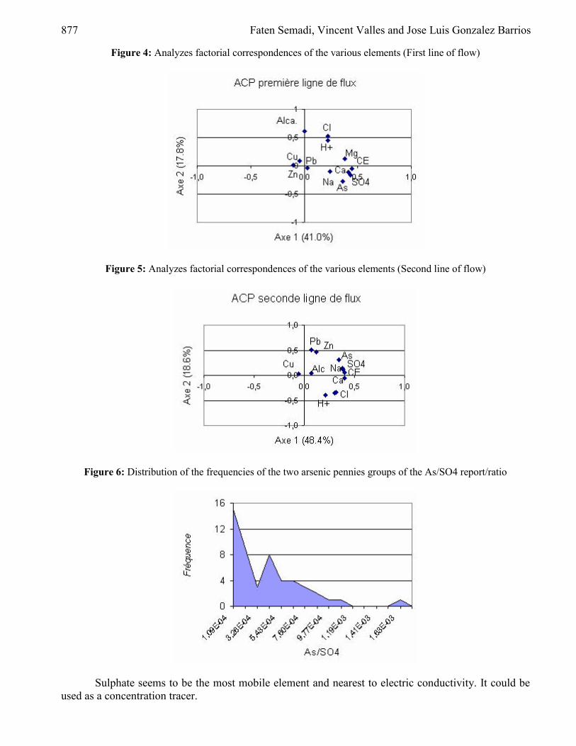
877 Faten Semadi, Vincent Valles and Jose Luis Gonzalez Barrios
Figure 4: Analyzes factorial correspondences of the various elements (First line of flow)
Figure 5: Analyzes factorial correspondences of the various elements (Second line of flow)
Figure 6: Distribution of the frequencies of the two arsenic pennies groups of the As/SO4 report/ratio
Sulphate seems to be the most mobile element and nearest to electric conductivity. It could be used as a concentration tracer.

Toxicity of Arsenic in the Ground Water of Comarca-Lagunera (Mexico) 878
Geochemical approach
Concentration diagrams: the aridity effect The concentration diagrams let classify water by increasing concentrations. When an element concentrates proportionally to the solution volume reduction, the slope of its dots is 1. This behaviour like a chemical tracer has not reaction between mineral and liquid phases. In this study case, the sulphate ion as well as sodium, chloride, magnesium and arsenic ions looks like tracers in a first approximation (fig.7). The arsenic content evolves mainly by concentration; it seems that there are not mineral precipitations limiting its concentration increasing; this can be related to the climate aridity. However the slope concentrations for chloride and sodium are lower than 1. This means that, from weak concentrations, the increasing concentrations for sodium are not completely proportional to the variation of the solution concentration factor; this mechanism implies probably ADSORPTION by clays. This phenomenon is very frequent in this salt environment studied by Gonzalez Barrios (1992). It is accompanied by a magnesium ADSORPTION process. The chloride behaviour can be related to its formation of iron oxi-hydroxides (green rusts) with partial substitution of OH- ions (Trolard, F et al., 1996, Condom, N. 2000). However, the intensity of this control is light.
In this group of chemical elements, magnesium and arsenic present a strong dispersion of observed points around the average tendency. Concerning arsenic, it was possible to treat separately two groups of points based on As/SO4 ratios which can be separated statistically. The bimodal character of the As/SO4 ratio frequencies (fig 6) makes possible to separate these two sub-groups.
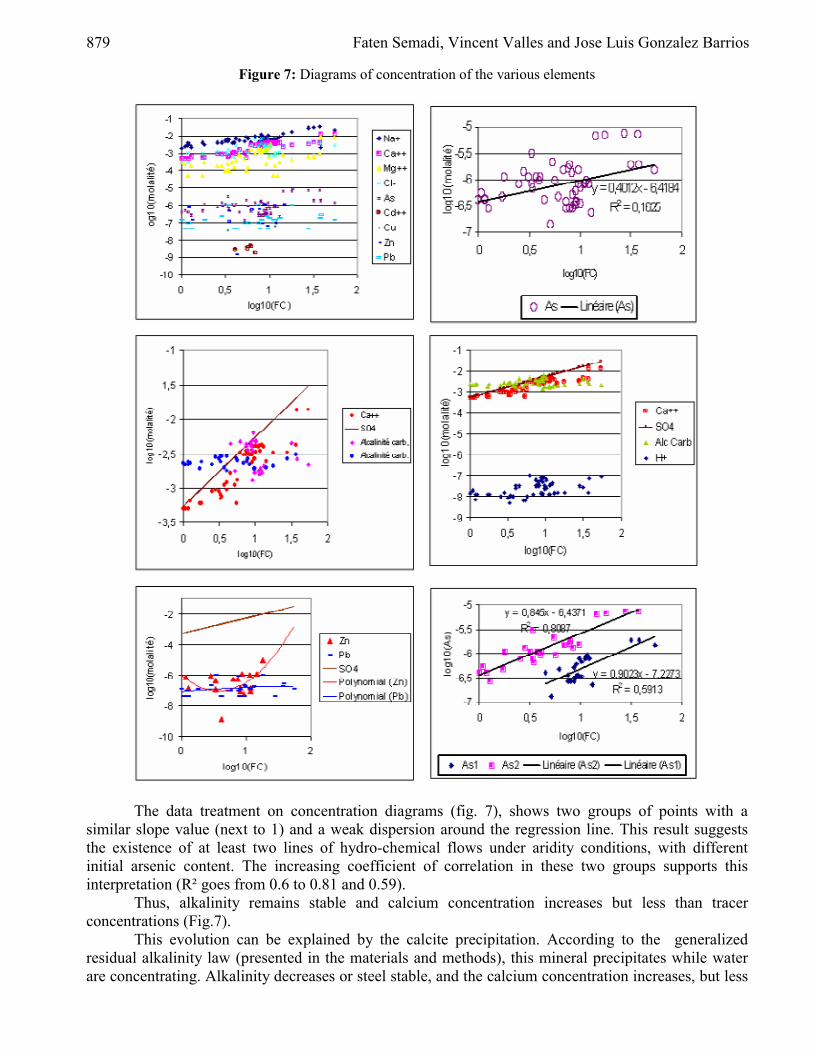
879 Faten Semadi, Vincent Valles and Jose Luis Gonzalez Barrios
Figure 7: Diagrams of concentration of the various elements
The data treatment on concentration diagrams (fig. 7), shows two groups of points with a similar slope value (next to 1) and a weak dispersion around the regression line. This result suggests the existence of at least two lines of hydro-chemical flows under aridity conditions, with different initial arsenic content. The increasing coefficient of correlation in these two groups supports this interpretation (R² goes from 0.6 to 0.81 and 0.59).
Thus, alkalinity remains stable and calcium concentration increases but less than tracer concentrations (Fig.7).
This evolution can be explained by the calcite precipitation. According to the generalized residual alkalinity law (presented in the materials and methods), this mineral precipitates while water are concentrating. Alkalinity decreases or steel stable, and the calcium concentration increases, but less

Toxicity of Arsenic in the Ground Water of Comarca-Lagunera (Mexico) 880
than the concentration factor. This is in conformity with the results obtained. The precipitation of calcite will be confirmed with the balance diagram of solution/calcite.
With constant CO2 content the reduction of alkalinity should increase the pH, by a reduction of the H+ content. In deed the mol concentration of this element increases with water concentration. It should be explained by a gradual concentration of CO2 in water which reflecting a space variability of the water tables. Indeed, when the medium is under water the gases exchanges are reduced. It results a weak content of O2 and a high content of CO2.
The data concerning metals like Zn, Pb, Cd and Cu are limited and interpretation will be related primarily to Zn and Pb that are elements better know (Fig.7). The lead concentrations are remarkably stables, the slope of the fitted points is close to 0, reflecting a mechanism of strong chemical control of Pb concentrations. It is probably the result of a mineral precipitation (oxyde/hydroxyde or sulphate kind). The study of balance diagrams will let to identify the kind of this mineral precipitation. Concerning the zinc, its variability is more important than Pb and its concentration tendency is less stable. This must be due to mineral precipitation as well, but less systematic than lead.
The concentration diagrams show the global concentration of water from upstream to downstream into hydrological flows. Chemical mechanisms of mineral precipitations are suggested but they must be confirmed by the balance diagrams. Conclusion This work is based on the analysis of 51 groundwater samples of the Comarca Lagunera region of northern arid of Mexico exposed to a health risk because of high arsenic concentration in groundwater used for irrigation and some of them for drinking water under rural and marginal conditions.
The methods used from statistics to chemical equilibrium modelling and sanitary risk assessment, allow to quantify the health risk and its variability.
The origin of arsenic pollution seems to be from dissolution of deep volcanic rocks in the mountains. The importance of this dissolution is variable according to lithological characteristics of the catchments. This induces geographical differences for the health risk assessment. Moreover the climate aridity causes water evaporation and concentration of soluble salts such as arsenic. The statistical approach shows that climate aridity is the main process related to high arsenic contents observed in this area. This is reflected in a health risk that increases from upstream to downstream where low areas are located.
When groundwater goes from upstream to downstream it transit by different ventilation conditions: good conditions upstream and bad conditions downstream. This causes a differential expression of dissolved arsenic forms. Trivalent forms are more toxics than pentavalent forms and become dominants downstream where the highest arsenic concentrations are observed.
In summary, it was possible to identify the origin of arsenic pollution, the main process responsible for its variability and the induced risk on the catchments area. Health risk related to arsenic is different upon the catchments area. However, the lack of referenced data concerning specific toxicity of arsenic forms, beyond the simple distinction between pentavalent and trivalent forms, does not let to validate the accurate health risk assessment obtained with thermodynamic models. This point could be a research line for the continuation of this work.

881 Faten Semadi, Vincent Valles and Jose Luis Gonzalez Barrios
References [1] Al-Droubi, A., 1976. Geochemistry of salts and the solutions concentrated by evaporation -
Model thermodynamic of simulation application on the salted ground of Chad, Th Doc. Sci., Univ. Of Strasbourg, France, 177 pages.
[2] Condom, N. 2000. Study and modeling of the transfers of water and aqueous solutions in the sodic grounds and the tablecloths of the Office of Niger to Mali. Thesis ENSAM, 180 pages. Dolique, R. 123PP. 1968-L' arsenic and its compounds. Published by the university presses of France.
[3] Gonzalez-Barrios, J.L., 1992. Water of irrigation and salinity of the grounds in Mexican arid region: example in "Comarca Lagunera", Th Doc. Sci., University of Montpellier II, France, 316 pages.
[4] Ribolzi, O, Valles, V and Bariac, T, 1996. Comparison of hydrograph deconvolutions using residual alcalinity, chloride and oxygen 18 aces hydrochemical tracers. Resour Toilets. LMBO, 32, 4, 1051-1059.
[5] Trolard F, Génin J.M.R., Abdelmoula Mr., Bourrié G, Humbert B and Herbillon A. (1997) Identification of green rust in A reductomorphic soil by Romance Mössbaner and spectroscopiés. Géochimica and Casmochimica Acta, 61, 1107-1111.
[6] Valles V and A.M. of Cockborne - 1992- Development of a software of geochemistry applied to the study cde the quality of water. Seminar "Deterioration and restoration of the quality of inland waters" Port-Leucate October 1-2, 1992, 20-23.
[7] Valles V, M Rezagui, L Auque, A Semadi, L Roger, H. Zougari, 1997. Geochemistry of saltworks slois in two arid zones of the Mediterranean basin. Geochemistry of the Chott Melghir-Mehrouane watershed in Algeria. Arid Soil Research and Rehabilitation (the USA): 11:71-84.

European Journal of Scientific Research ISSN 1450-216X Vol.20 No.4 (2008), pp.882-890 © EuroJournals Publishing, Inc. 2008 http://www.eurojournals.com/ejsr.htm
Modeling and Temperature Controller Design for
Yazd Solar Power Plant
Aref Shahmansoorian Islamic Azad University of IEslamshahr E-mail: [email protected]
Abdolvahed Saidi
National Iranian Oil Company-OGPC Department E-mail: [email protected]
Abstract
The Yazd Integrated Solar Combined Cycle (ISCC) Power Plant consists of two gas turbines that are generating power synchronous to Iranian national electrical network. One steam turbine will be supplied by gas units, while a parabolic through solar field is integrated with the system, as a combined cycle. In this paper an integrated model of the solar field with the purpose is presented, and a multivariable generalized predictive temperature controller is proposed for the system. As it is illustrated in the simulation results, such a control strategy can robustly regulate both the temperature of outlet oil, and the temperature of outlet steam water of the solar boiler, despite the variation of the inherent time delays of the system and external disturbances. Keywords: ISCC power plant, Solar Field, heat exchanger, modeling, multivariable GPC.
I. Introduction The feasibility studies and technical specification of an integrated solar combined cycle power plant has been recently completed, and this type of power plant will be constructed in the city of Yazd in near future [15]. This power plant is designed with two steam turbines, two gas turbines and a solar field which supplies excess steam for steam turbines. The solar field consist of parabolic through collectors, solar boiler, pumps, control valves and an expansion vessel. The solar field itself possess 84 loops with eight collectors in each loop[16]. The collector has parabolic mirrors which focus the sun beams directly on the oil pipe, and the solar collectors are equipped with a sun tracker system. The oil enters the solar field with the temperature of 230ºC and depart from it with the temperature of 391ºC. The outlet oil from solar field enters a special heat exchanger named solar boiler, in which the accumulated heat in the solar field exchanges the supplied water into superheated steam[17].
The solar boiler consist of three exchangers that preheating, evaporating and superheating the water in three stage. The oil enters the superheater stage at 391ºC/15bar and depart from preheater stage at 293ºC/11bar. The supplied water enters the preheater with 235ºC/105bar and depart the superheater with 380ºC/102 bar. The inverse direction heat exchanger is chosen in order to increase the rate of heat transfer. The necessary pressure for oil is provided with 3 pumps, which one of them is standby. The type of tank in the solar field is an expansion vessel that the inlet pressure is fixed with

Modeling and Temperature Controller Design for Yazd Solar Power Plant 883
nitrogen. The control valves are regulating the oil flow for temperature control. Figure (1) illustrates the schematics of an ISCC power plant [12].
Figure 1: Integrated Solar Combined Cycle Power Plant
II. Solar Field Modeling In order to have a tractable and complete model of the solar field it is necessary to model the heat exchanger and the solar collectors in detail [1]. In this section the proposed models for these components are studied. A. Solar Collector Model
The designed solar collector consists of double steel/glass pipe with vacuum insulation. The collector mirrors absorb a fraction of solar beam energy, and focuses the rest on the aforementioned oil pipes at the center of parabolic through. The heat energy is transferred to the oil through convection, conduction and radiation [14].
Figure 2: circuit model of heat transfer
Since the radiation heat transfer relates the rate of heat transfer to the fourth power of the temperature, in order to compensate for the temperature losses, a global coefficient of thermal losses is defined as below:
)( ambs
lossl TT
QH−
= (1)
In which sT and ambT are the oil pipe surface and the ambient temperatures, respectively. The Heat loss factor, lH can be obtained from calibration experiments, and can be assumed constant with a sufficient degree of accuracy. Considering the heat loss in the collectors as elaborated, the dynamic equation of solar field heat transfer is given as following [4]:
)()( fstambslopts
sss TTLHTTGHIGt
TAC −−−−=∂∂ ηρ (2)
This equation contains the absorbed energy of the oil pipe, the transferred energy to the oil and the heat loss to ambient. The left hand side of the equation determines the temperature variation of the metal pipe surface, in the condition while the thermal equilibrium has not been reached. The first term

884 Faten Semadi, Vincent Valles and Jose Luis Gonzalez Barrios
in the right hand side determines the volume of radiation energy that oil pipe has received, the second term shows the ambient heat loss, and the third term evaluates the oil absorbed energy. The amount oil absorbed energy can be determined by the following [4]:
)( fstf
fff
fff TTLHx
TqC
tT
AC −=∂
∂+
∂
∂ •ρρ (3)
In this equation the first term in LHS governs the temperature variation of the oil with respect to time, and the second term governs the temperature variation with respect to the movement of oil. Since the governing heat transfer equations are partial differential equations, for the purpose of control they are discretized with the assumption of the temperature being fixed along each collector, using finite element method.
)()(
)()(. 1
fsfff
tff
ff
f
fssss
ambsssssss
opts
TTAC
LHTTA
mt
T
TTAC
KTTAC
KIACG
tT
−+−=∆
∆
−−−−=∆∆
−
•
ρρ
ρρρη
(4) B. Heat Exchanger Model
In order to model the heat exchanger, the inlet pressure is assumed to be constant [12,14]. The governing equations can then be classified into two set of equations for temperature variations and phase variations. It is assumed that in the preheater and superheater stages, there are no phase change, and hence, the governing equations are due to the temperature variation. In the preheater there is only temperature rise in water, while in superheater the temperature increase occurs on the steam [17]. The boiler design conditions guarantees that the water is entering the preheater with the temperature of 293ºC and will depart it with the temperature of 314ºC. In steam generator water exchange to steam with the temperature of 314ºC and in superheater saturated steam is heated to the temperature of 380ºC. Note that the governing equation of heat exchanger is also in the form of partial differential equation. For control purpose the governing equations are discretized using finite element method with three nodes. The governing equation of oil behavior in each node is as follows [13, 18]:
( ) ( )
( ) ( ) ( ) ( )
( ) ( )
( ) ( )
( )
( ) ( )
oiloil oil oil oil oil oil oil out oil in
oil out water out oil in water in
oil out water out
oil in water in
dTV C C F T Tdt
K T T T T
T TLn
T T
ρ ρ= −
⎡ ⎤− − −⎣ ⎦−⎛ ⎞−⎜ ⎟⎜ ⎟−⎝ ⎠
(5)
the left side term of the above equation showes the temperature variation of oil in time, the first term of right, show the temperature variation of oil in effect of moving oil between pipes of energy absorber in any stage. The second term of right side shows the rate of heat transfer from oil to water. The equation that gives the thermodynamical behavior of water (steam) in pre heater and super heater is shown as equation (6).
In which it is assumed that the temperature in those stages are fixed and only temperature variations occurs at the transient of one stage to another. Similarly, the equation that gives the thermodynamical behavior of water (steam) in preheater and superheater in this case, is [13, 18]:
( ) ( )
( ) ( ) ( ) ( )
( ) ( )
( ) ( )
( )
( ) ( )
waterwater water water water water water water out water in
oil out water out oil in water in
oil out water out
oil in water in
dTV C C F T Tdt
K T T T T
T TLn
T T
ρ ρ= − −
⎡ ⎤− − −⎣ ⎦+⎛ ⎞−⎜ ⎟⎜ ⎟−⎝ ⎠
(6)
In the equation (6) we assume that temperature in each section is fixed (temperature is variation just in cross from section to another section). It should be considered that in this equation, the physical characteristic of water in pre heater has been assumed fixed because of the small variation in these parameters.

Modeling and Temperature Controller Design for Yazd Solar Power Plant 885
In this equation the physical properties of the water is assumed to be fixed in the preheater. Whereas, the physical properties of steam in the superheater show larger variation, and hence, must be taken into account. To include this variation into the system dynamics the changes of ,C ρ (density and specific thermal capacity) is considered by the following equations into the model. (For a detail discussion on the modeling refer to [6].
).
.(3145.8
18
KkmolmkNR
RRRTP
steam
=
==ρ (7)
θθθ 6989.3751.8254.18305.143 5.025.0 −+−=C (8)
100/)(015.18
KelvinT
CC steam
=
=
θ
(9)
The equation that gives the thermo-dynamical behavior of saturated steam in steam generator is shown in the equation (10):
[ ] ( )••• +−=
−−
−−− umhmhm
TTTT
Ln
TTTTKcviioo
cH
cH
cHCH
)(
)()(
12
21
12212 (10)
••• −= cvio mmm In this equation •
im , •om , cvm• are flow of inlet water, flow of outlet water and variation of
control value respectively. h is enthalpy of steam and u is energy of mass unit. The left side term of above equation is rate of heat transfer from oil to water. The first two terms of right, showes the variation of thermal power of saturated steam in cross of control value, and the last term showes the variation of energy in control volume [9, 10]. III. Controller Synthesis The solar field is a nonlinear, multivariable system possessing long and varying time delays. For this class of systems the predictive control methods are suitable. These types of controller are the most attractive controllers for process control practitioners, after common PID controllers [3, 7]. In this paper a multivariable GPC routine is proposed for temperature control of the system. The time delay in the system is caused by the installation distance ( x ) between the actuators and the sensors in the system. Hence, the time delay is related to the fluid speed and distance between the sensor and pump, as follows:
ντ x=
•••
••
∑===⇒
=⇒==
mV
mV
mAx
AmAvQm
iiρρρτ
ρνρρ
(11)
A. System Identification and parameter estimation
The solar field is a two-input two output system, from a control point of view. The system inputs are the oil and water flow rates and its outputs are the oil and water temperatures. From the well known identification techniques, the transfer matrix of the system can be obtained from simulated input output pairs of the system. The identified model of the system has been derived as following:

886 Faten Semadi, Vincent Valles and Jose Luis Gonzalez Barrios
⎥⎥⎥⎥
⎦
⎤
⎢⎢⎢⎢
⎣
⎡
++
+=−
−
−−
−
−
−−
−
−
2221
11
122
122
121
121
111
111
1
1
0
1
1)('dd
d
zzT
zkz
zTzk
zzT
zk
zG (12)
As it is clear from the structure of the identified model, the water temperature is almost not related to the outlet oil temperature (G12=0), and this weak relation can be modeled as a disturbance to the system. The other components are simply modeled with a first order system with a time varying time delay. This structure of the model can be used for the GPC synthesis. B. Design of multivariable GPC controller
The controller design consists of three steps. A) prediction model determination. B) Objective function assignment and C) control law calculation. The prediction model for the system can be derived from the equation (12), in which the model is rewritten in the form of :
∆+−= −− )()1()()()( 11 tetuqBtyqA (13)
In which )(tu is control signal and )(ty is the process output as the vector of oil and water temperatures. Moreover, )(te is measurement noise with zero mean and 11 −−=∆ q . )( 1−qA , )( 1−qB are the polynomial matrices with degree An and Bn respectively. The Objective function to be minimized has the form of :
[ ] [ ]∑ ∑∑= == ⎭
⎬⎫
⎩⎨⎧
−+∆++−+=m
i
N
j
N
jiii
u
jtujtwjtyrJ1 1
2
1
2 )1()()(2
λ (14)
Or in matrix form: [ ] [ ] uuwyRwyJ TT ∆∆+−−= λ (15)
In which 2N is the maximum of prediction horizon and uN is the control horizon. λ is the
penalty coefficient and R is the weighting matrix of errror signal. In order to generate the control signal, the future outputs of the system is predicted by the following equation:
y G u f= ∆ + (16) In which, f is the free response of the system and G includes the step response parameters.
The optimal solution for the control signal to minimize the cost function (15), while preserving closed loop stability is calculated from the following equation.
[ ] 10 0 ( )T Tu I G RG I RG w fλ
−⎡ ⎤∆ = + −⎣ ⎦L (17)
C. Parameter Tuning in Multivariable GPC
The tuning of the controller parameters is mostly based on experience, and the simulation of the closed loop response. The designer has the freedom to tune either the cost function weighting, or change the disturbance dynamics, observer dynamics, the desired trajectory and finally the prediction and control Horizons. More penalizing λ on the control effort and R on the tracking error will reduce the control effort. The structure of the model is fixed in this method and only the noise levels can be assigned to tune the performance. However, from the inherent integrator form of )()1()( 111 −−− −= zAzzD forces the error of the closed loop system to a step disturbane to converge asymptotically to zero [8, 11]. IV. Closed-Loop Simulation Result The designed controller for the system has the parameters 1 26, 37, 3uN N N= = = and the weighting functions are tuned through the simulation to:
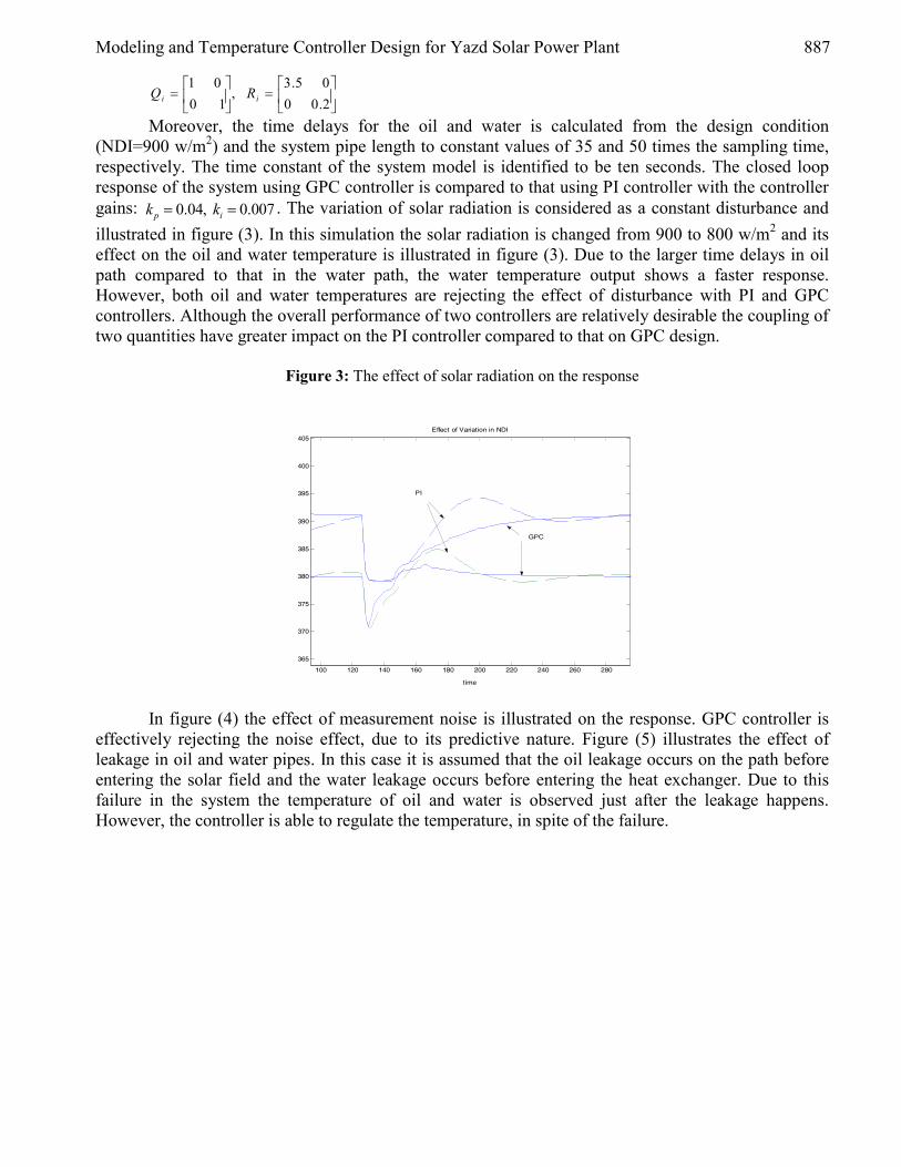
Modeling and Temperature Controller Design for Yazd Solar Power Plant 887
⎥⎦
⎤⎢⎣
⎡=⎥
⎦
⎤⎢⎣
⎡=
2.0005.3
,10
01ii RQ
Moreover, the time delays for the oil and water is calculated from the design condition (NDI=900 w/m2) and the system pipe length to constant values of 35 and 50 times the sampling time, respectively. The time constant of the system model is identified to be ten seconds. The closed loop response of the system using GPC controller is compared to that using PI controller with the controller gains: 0.04, 0.007p ik k= = . The variation of solar radiation is considered as a constant disturbance and illustrated in figure (3). In this simulation the solar radiation is changed from 900 to 800 w/m2 and its effect on the oil and water temperature is illustrated in figure (3). Due to the larger time delays in oil path compared to that in the water path, the water temperature output shows a faster response. However, both oil and water temperatures are rejecting the effect of disturbance with PI and GPC controllers. Although the overall performance of two controllers are relatively desirable the coupling of two quantities have greater impact on the PI controller compared to that on GPC design.
Figure 3: The effect of solar radiation on the response
100 120 140 160 180 200 220 240 260 280
365
370
375
380
385
390
395
400
405
time
Effect of Variation in NDI
PI
GPC
In figure (4) the effect of measurement noise is illustrated on the response. GPC controller is effectively rejecting the noise effect, due to its predictive nature. Figure (5) illustrates the effect of leakage in oil and water pipes. In this case it is assumed that the oil leakage occurs on the path before entering the solar field and the water leakage occurs before entering the heat exchanger. Due to this failure in the system the temperature of oil and water is observed just after the leakage happens. However, the controller is able to regulate the temperature, in spite of the failure.
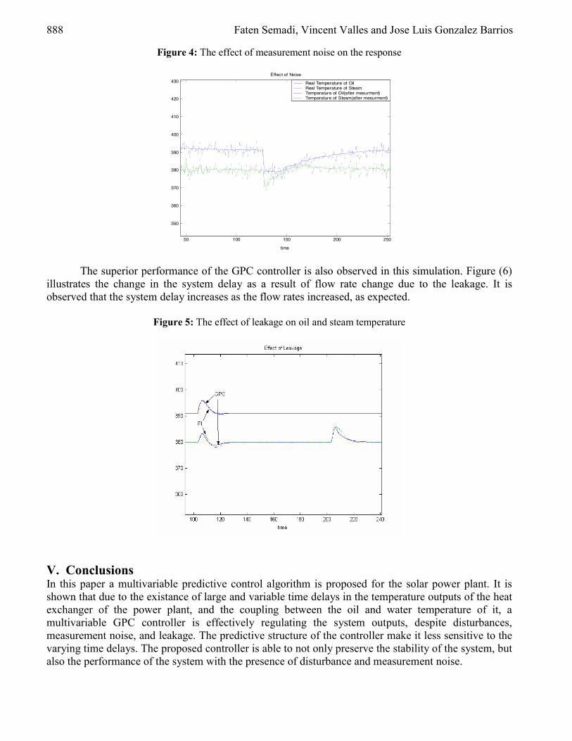
888 Faten Semadi, Vincent Valles and Jose Luis Gonzalez Barrios
Figure 4: The effect of measurement noise on the response
50 100 150 200 250
350
360
370
380
390
400
410
420
430
time
Effect of Noise
Real Temperature of OilReal Temperature of SteamTemperature of Oil(after mesurment)Temperature of Steam(after mesurment)
The superior performance of the GPC controller is also observed in this simulation. Figure (6) illustrates the change in the system delay as a result of flow rate change due to the leakage. It is observed that the system delay increases as the flow rates increased, as expected.
Figure 5: The effect of leakage on oil and steam temperature
V. Conclusions In this paper a multivariable predictive control algorithm is proposed for the solar power plant. It is shown that due to the existance of large and variable time delays in the temperature outputs of the heat exchanger of the power plant, and the coupling between the oil and water temperature of it, a multivariable GPC controller is effectively regulating the system outputs, despite disturbances, measurement noise, and leakage. The predictive structure of the controller make it less sensitive to the varying time delays. The proposed controller is able to not only preserve the stability of the system, but also the performance of the system with the presence of disturbance and measurement noise.

Modeling and Temperature Controller Design for Yazd Solar Power Plant 889
Figure 6: The Variation of delay in effect of flow variation
VI. Nomenclature
sρ Density of oil pipe (kg/m3) •q Oil flow (m3/s)
Cs Specific thermal capacity of oil pipe (J/kg ºC) G Width of collector (m) As Area of metal pipe (m2) Ht Heat transfer coefficient from pipe to oil (W/m2 ºC)
fρ Density of oil (kg/m3) L Inner diameter of oil pipe (m)
fC Specific thermal capacity of oil (J/kg ºC) I Sun direct radiation (W/ m2) V Volume of fluid path (m3)
•m Mass flow of fluid(kg/s) Af Inner cross area of oil pipe (m2) Tf Oil temperature along one collector (ºC) Tf
- Oil temperature along previous collector (ºC) Ts Temperature of oil pipe (ºC)
optη Optical efficiency of mirrors x Distance of sensor from control valve (m) HL Thermal loss coefficient (W/m2 ºC) v Oil velocity (m/s) ρ Fluid density(kg/m3) Q Flow (m3/s) A cross area of fluid pipe (m2)

890 Faten Semadi, Vincent Valles and Jose Luis Gonzalez Barrios
References [1] A.W. ordys – A.W. pike - M. A. Johnson – R.M.katebi and M.J.Grimble.“Modeling and
simulation of Power Generation Plants” Springer-verlag 1994 [2] A.Saidi “Solar Field Modeling and Temperature Control of Yazd ISCC Power Plant” Master
thesses, K.N.Toosi,University of technology,2002 [3] Donna M.Schneider “Control of Process with Time Delays” IEEE Transactions on Industry
Applications Vol.24No.2,March/Appril-1988 [4] E.F Comacho – M. Berenguel and F.R. Rubio. “Advanced Control of Solar Plant” Springer-
verlag 1997 [5] E.F.Camacho and C.Bordons “Model Predictive Control in the Process Industry” Springer-
Verlag,1995 [6] Gordon van wylen- Richard Sonntag- claus Borgnakke “Fundamentals of Classical
Thermodynamics” fourth Edition [7] J.E. Marshall “Control of time – delay systems.” Institution of Electrical Engineers 1979 [8] J.M.Maciejowski “Predictive Control with constraint” Prentice Hall-2002 [9] Jonas Eborn and Karel Johan Astrom. “Modeling of a Boiler Pipe with Two-Phase Flow
Instabilities” www.control.lth.sel~kja/rodpaper.pdf [10] K.J Astrom – R.D. Bell. “Drum – Boiler Dynamics”1998 www.control.lth.sel~kja/rodpaper.pdf [11] O.Bego,N.Peric “Decoupling Multivariable GPC with Reference Observation” 10th
Mediterranean Electrical Conference, MeleCon 2000,Vol. II [12] Pilkington (Solar International) “Status Report on Solar Thermal Power Plants”. www.
Pilkington .com [13] Pierre Bélanger “Control engineering: a modern approach” Saunders College Pub.1995. [14] Sandia Co. “Test Results SEGS LS-2 Solar Collector” Technical Report www.Sandia.gov.
1994 [15] S.R.Hosseini “Report of feasibility study (Technical and Economical) of yazd solar thermal
power plant” NRI.2000 [16] S.R.Hosseini “Report of solar field design in yazd solar thermal power plant” NRI.2000 [17] S.R.Hosseini “Report of solar boiler design in yazd solar therma power plant” NRI 2000 [18] V.Ganapathy “Steam Plant Calculation Manual.” Marcel Dekker1984

European Journal of Scientific Research ISSN 1450-216X Vol.20 No.4 (2008), pp.891-904 © EuroJournals Publishing, Inc. 2008 http://www.eurojournals.com/ejsr.htm
A Predictive Current Control Technique on Fuel Cell Based Distributed Generation in a Standalone AC Power Supply
K. G. Firouzjah Faculty of Electrical & Computer Engineering, Noshirvani University of Technology
Shariati Street, Babol, Iran, P. O. Box 47135-484 E-mail: [email protected]
Tel: +98-111-323-9214; Fax: +98-111-323-9214
H. Eshaghtabar Faculty of Electrical & Computer Engineering, Noshirvani University of Technology
Shariati Street, Babol, Iran, P. O. Box 47135-484 Tel: +98-111-323-9214; Fax: +98-111-323-9214
A. Sheikholeslami
Faculty of Electrical & Computer Engineering, Noshirvani University of Technology Shariati Street, Babol, Iran, P. O. Box 47135-484 Tel: +98-111-323-9214; Fax: +98-111-323-9214
S. Lesan
Faculty of Electrical & Computer Engineering, Noshirvani University of Technology Shariati Street, Babol, Iran, P. O. Box 47135-484 Tel: +98-111-323-9214; Fax: +98-111-323-9214
Abstract
This research presents a new method based on predictive current control (PCC) of fuel cell based distributed generation systems (DGS) in a standalone AC power supply. To boost low output DC voltage of the fuel cell to high DC voltage and compensate for its slow response during the transient, two full-bridge DC to DC converters are adopted and their controllers are designed based on PCC. The proposed method produces the reference current by using of the DC link capacitor voltage. Thereupon the method determines the portion of fuel cell and backup battery to feed load and capacitor. The analysis results presented in this research demonstrate that the suggested method is capable to increase transient performance of adopted system in load and fuel cell output voltage variations. Simulations with MATLAB have been carried out to verify the proposed predictive current controller in mentioned application and the results are discussed in this research. Keywords: Fuel Cell, Distributed Generation, Predictive Current Control, DC-DC
Converters, Backup Battery
A Predictive Current Control Technique on Fuel Cell Based Distributed Generation in a Standalone AC Power Supply 892 1. Introduction Previous empirical research provides contradictory and inconclusive evidence on the value relevance of comprehensive income disclosures promulgated in different countries. Thus, present study using comprehensive income of Iranian firm's data shed more lights on the issue.
Fuel cells are devices capable of converting chemical energy into heat and dc electrical energy by means of the oxidation of a fuel, usually hydrogen (Padulles et al, 2000). Distributed generation (DG) technologies can provide energy solutions to some customers that are more cost-effective, more environmentally friendly, or provide higher power quality or reliability than conventional solutions. The voltage of fuel cell stack decreases largely as the load current increase, and the voltage increases as the temperature increase at the same current. Thus DGS should be interfaced with Power Electronic systems such as DC to DC or/and DC to AC power converters to obtain a sinusoidal AC output voltage with fixed frequency from variable or high-frequency AC voltage sources or DC voltage sources (Haiping et al, 2005). So the DC-DC converter plays a key role in making the fuel cell DC power available for stand-alone applications.
To boost low output DC voltage of the fuel cell to high DC voltage, a forward DC to DC boost converter, a push-pull DC to DC boost converter or an isolated full-bridge DC to DC power converter can be selected. In addition, various topologies such as the H-bridge series resonant buck and boost converters have been presented in (Blaabjerg et al, 2004). Anderson et al, (2002) present a current fed push-pull converter. This topology decreases the conduction losses in the switches due to the low fuel cell voltage. Nergaard et al, (2002) suggest an interleaved front-end boost converter. This topology considerably reduces the current ripple flowing into the fuel cell. A dual loop control strategy (current and voltage loop) has been used for the interleaved converter. Jung et al, (2005;2005) introduce a Z-source converter. This is a new concept in which a shoot-through vector directly steps up the DC source voltage without using a boost DC-DC converter. The boost voltage rate depends on the total duration of the shoot-through zero vectors over one switching period Jung et al, (2005). Also, In reference (Wang and Nehrir, 2006) a non-isolated boost converter with a conventional PI controller has been used for the converter control. Akkinapragada (2007) had been employed a non-isolated buck-boost DC-DC converter with a closed loop PWM (pulse width modulation) control strategy as described in Reference (Mohan et al, ). The reference (Duran-Gomez et al, 2006) had been presented an approach to convert the generated dc output voltage of a PV cell array into a higher regulated dc voltage. The approach employs a series-combined connected boost and buck boost dc-dc converter for power conditioning of the dc voltage provided by a photo-voltaic array. Chandrasekaran and Gokdere (2004) introduce a novel composite integrated magnetic (IM) core structure, which minimizes inductor current ripple. Their subject is a compact, IM core structure for a three-phase interleaved, DC-DC boost converter that feeds off the fuel cell output and can provide a programmable, regulated, high voltage DC bus for the distributed power system.
In recent years, the higher efficiency and the more advanced power conversion, energy utilization equipment, a variety of circuit topologies of the soft-switching DC-DC power converter are urgently required. The reference (Ogura et al, 2003) has introduced a boost type ZVS-PWM chopper-fed DC-DC power converter with a single active auxiliary resonant snubber in the load side for the power interface of solar photovoltaic and fuel cell power conditioners. The character of this boost type ZVS-PWM chopper-fed DC-DC power converter is feasible. Also, a unidirectional isolated full-bridge DC to DC power converter can be used to boost low fuel cell voltage (Bendre et al, 2003; Aydemir, 2002; Kim et al, 1997; Jain et al, 2002; Brunoro and Vieira, 1999; Jeon and Cho, 2001). In addition, a bidirectional full-bridge DC to DC power converter can be used for stepping up low battery voltage or stepping down high-voltage-side DC link according to battery discharge or recharge mode (Peng et al, 2004; Jiang and Dougal, 2003). Among the presented power converters, two phase-shifted full-bridge DC to DC converters, which are one of the most attractive topologies for high power generation are adopted as described in (Jung, 2005; Keyhani and Jung, 2004) with a unidirectional full-bridge DC to DC boost converter for the fuel cell and a bidirectional full-bridge DC to DC boost/buck converter for

893 K. G. Firouzjah, H. Eshaghtabar, A. Sheikholeslami and S. Lesan
battery. This research develops a circuit model and controllers of fuel cell based distributed generation systems (DGS) in a standalone AC power supply. Dynamic model of the fuel cell is considered. To boost low output DC voltage of the fuel cell to high DC voltage and compensate for its slow response during the transient, two full-bridge DC to DC converters are adopted and their controllers are designed. Furthermore, (Suzuoka et al, 2003) presents a novel circuit topology of a voltage source type zero voltage soft-switching full bridge inverter DC-DC power converter with an isolated high-frequency transformer link this power converter incorporates zero current soft-switching (ZCS) mode phrase-shifted PWM active power switches in series with diode into two diode arms of full-bridge rectifier or center-tapped rectifier in transformer secondary-side.
In spite of desirable performance of the mentioned methods, a novel method based on predictive current control has been proposed to control the fuel cell and backup battery on the presented structure in (Jung, 2005; Keyhani and Jung, 2004). The proposed method produces the reference current by using of the DC link capacitor voltage. In other word, the presented algorithm calculates the required current of load and capacitor to regulate and control DC output at a desired voltage level. Thereupon the method determines the portion of fuel cell and backup battery to feed load and capacitor. In this research, the predictive current control strategy as described in References (Rodriguez, 2007; Rodriguez, 2004; Wen and Zheng, 2006; Premrudeepreechacharn and Poapornsawan, 2000) has been employed. 2. System Structure The adopted structure of fuel cell, backup battery and the interfaced converters are based on the reference (Jung, 2005; Keyhani and Jung, 2004) as described in Fig. 1. In this system, a low voltage DC output of fuel cell is used along with unidirectional boost converter to prevent reliability deterioration by stacking a number of series cells. A low DC voltage battery for backup is connected in parallel with the high side DC link through a bidirectional buck/boost converter because difficulties in battery management can be significantly reduced. Furthermore, an isolated full-bridge DC to DC power converter is adopted to boost low output DC voltage of fuel cell because its topology is suitable for high power applications. To boost low output DC voltage of the fuel cell to high DC voltage, a forward, a push-pull or an isolated full-bridge DC to DC power converter is selected. Among these power converters, two phase-shifted full-bridge DC to DC converters are consist of a unidirectional full-bridge DC to DC boost converter for fuel cell and a bidirectional full-bridge DC to DC boost/buck converter for the battery. In Fig. 1, the unidirectional power converter system for the fuel cell consists of a fuel cell, an input filter (L1, C1), a full-bridge power converter (F1 to F4), a high frequency transformer (N1:N2), a bridge-diode (DF1 to DF4), and an output filter (L2, C2), while the bidirectional power converter system for the battery consists of a battery, a static switch (SB), two full-bridge power converters (B1 to B4, B11 to B44), and a high frequency transformer (n1:n2) (Jung, 2005).
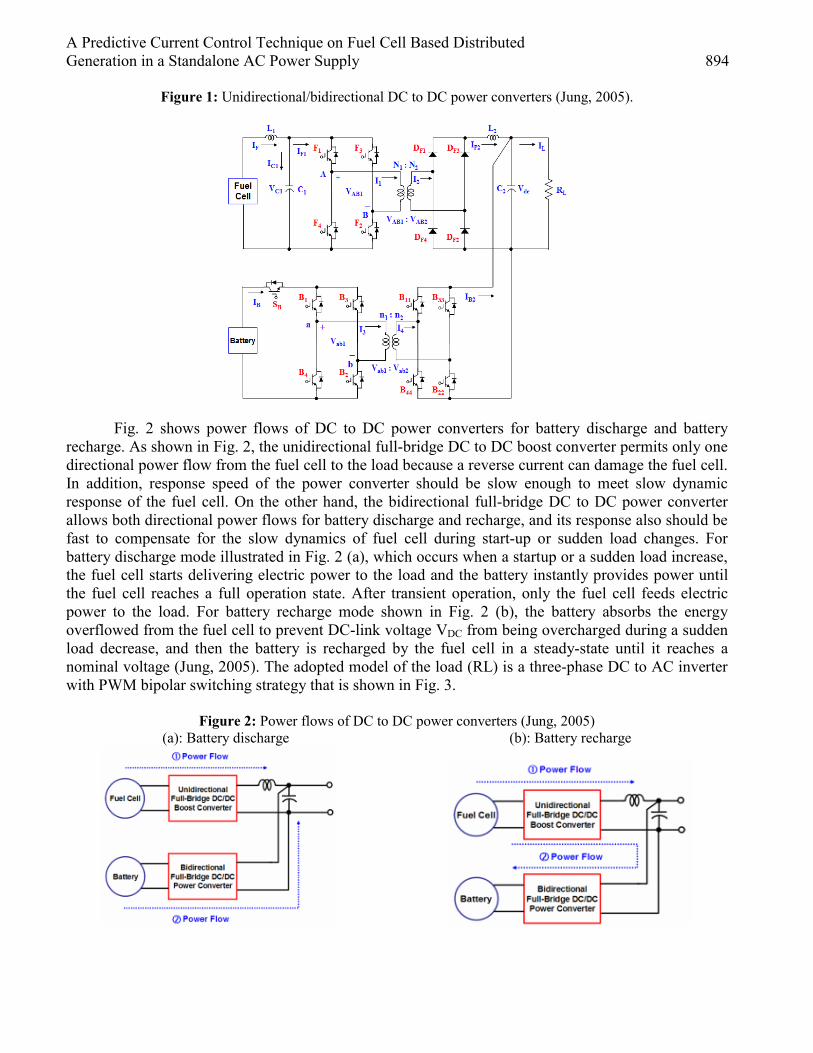
A Predictive Current Control Technique on Fuel Cell Based Distributed Generation in a Standalone AC Power Supply 894
Figure 1: Unidirectional/bidirectional DC to DC power converters (Jung, 2005).
Fig. 2 shows power flows of DC to DC power converters for battery discharge and battery recharge. As shown in Fig. 2, the unidirectional full-bridge DC to DC boost converter permits only one directional power flow from the fuel cell to the load because a reverse current can damage the fuel cell. In addition, response speed of the power converter should be slow enough to meet slow dynamic response of the fuel cell. On the other hand, the bidirectional full-bridge DC to DC power converter allows both directional power flows for battery discharge and recharge, and its response also should be fast to compensate for the slow dynamics of fuel cell during start-up or sudden load changes. For battery discharge mode illustrated in Fig. 2 (a), which occurs when a startup or a sudden load increase, the fuel cell starts delivering electric power to the load and the battery instantly provides power until the fuel cell reaches a full operation state. After transient operation, only the fuel cell feeds electric power to the load. For battery recharge mode shown in Fig. 2 (b), the battery absorbs the energy overflowed from the fuel cell to prevent DC-link voltage VDC from being overcharged during a sudden load decrease, and then the battery is recharged by the fuel cell in a steady-state until it reaches a nominal voltage (Jung, 2005). The adopted model of the load (RL) is a three-phase DC to AC inverter with PWM bipolar switching strategy that is shown in Fig. 3.
Figure 2: Power flows of DC to DC power converters (Jung, 2005) (a): Battery discharge (b): Battery recharge

895 K. G. Firouzjah, H. Eshaghtabar, A. Sheikholeslami and S. Lesan
Figure 3: Three-phase DC to AC inverter with Three-phase load.
3. Predictive Current Control (PCC) in Single Phase Converter Fig. 4 shows the topology of single phase full-bridge converter with nonlinear Inductive-Resistive load. Nonlinear treatment of load is modeled in the form of (e) potential. According to the Fig. 4, the current direction is being selected conventionally in a fix direction. If switching of converter selected as bipolar control, the switching states will be:
1 4 2 3
2 3 1 4
1 S ,S : S ,S : 2 S ,S : S ,S :
State on offState on off
→
→ Therefore, the duty cycle of S1,S4 switches (D) can be defined. While S1,S4 and S2,S3 are ON,
the load voltage will be equal to Vd and -Vd respectively. 1,4onT
DT
= (1)
Ton is the time that S1,S4 are ON in a period (T). So, in a sample the mean value of load voltage is equal to 2D-1, that:
(2 1) ddiD V Ri L edt
− = + + (2)
While S2,S3 are ON, the duty cycle is D'. According to the bipolar switching technique of single phase converter:
1D D′= − (3) By rewriting these equations in discrete time domain we have:
( 1) ( )( ) ( ) ( )
( )(2 -1) n n
n d n n
i iD V Ri L e
T+ −
= + + (4)
( 1) ( )( ) ( )
( )
( )
2
n nn n d
nd
i iRi L e V
TDV
+ −+ + +
= (5)
Figure 4: Single phase full-bridge converter with nonlinear load
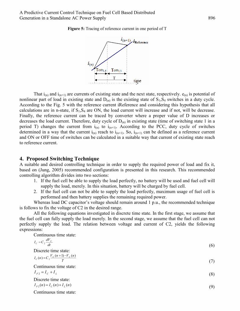
A Predictive Current Control Technique on Fuel Cell Based Distributed Generation in a Standalone AC Power Supply 896
Figure 5: Tracing of reference current in one period of T
That i(n) and i(n+1) are currents of existing state and the next state, respectively. e(n) is potential of nonlinear part of load in existing state and D(n) is the existing state of S1,S4 switches in a duty cycle. According to the Fig. 5 with the reference current iReference and considering this hypothesis that all calculations are in n-state, if S1,S4 are ON, the load current will increase and if not, will be decrease. Finally, the reference current can be traced by converter where a proper value of D increases or decreases the load current. Therefore, duty cycle of D(n) in existing state (time of switching state 1 in a period T) changes the current from i(n) to i(n+1). According to the PCC, duty cycle of switches determined in a way that the current i(n) reach to i(n+1). So, i(n+1) can be defined as a reference current and ON or OFF time of switches can be calculated in a suitable way that current of existing state reach to reference current. 4. Proposed Switching Technique A suitable and desired controlling technique in order to supply the required power of load and fix it, based on (Jung, 2005) recommended configuration is presented in this research. This recommended controlling algorithm divides into two sections:
1. If the fuel cell be able to supply the load perfectly, no battery will be used and fuel cell will supply the load, merely. In this situation, battery will be charged by fuel cell.
2. If the fuel cell can not be able to supply the load perfectly, maximum usage of fuel cell is performed and then battery supplies the remaining required power.
Whereas load DC capacitor’s voltage should remain around 1 p.u., the recommended technique is follows to fix the voltage of C2 in the desired range.
All the following equations investigated in discrete time state. In the first stage, we assume that the fuel cell can fully supply the load merely. In the second stage, we assume that the fuel cell can not perfectly supply the load. The relation between voltage and current of C2, yields the following expressions:
Continuous time state:
2C
CdVI Cdt
= (6)
Discrete time state:
2( 1) ( )( ) C C
CV n V nI n C
T+ −
= (7)
Continuous time state: 2F C LI I I= + (8)
Discrete time state: 2 ( ) ( ) ( )F C LI n I n I n= + (9)
Continuous time state:

897 K. G. Firouzjah, H. Eshaghtabar, A. Sheikholeslami and S. Lesan
22 2
FAB C
dIV L Vdt
= + (10)
Discrete time state: 2 2
2 2( 1) ( )( ) ( )F F
AB CI n I nV n L V n
T+ −
= + (11)
where: Re( 1) 1 . .C C fV n V p u+ = =
Also, the average voltage of VAB1, based on bipolar switching technique of full bridge power converter (F1 to F4), is as follow:
1 (2 1)AB FdcV D V= − (12) 2
1 2 2AB T T ABdIV L R I Vdt′
′ ′= + + (13)
That RT and LT are the transformer’s impedances. 1
2 22
AB ABNV VN
′ = (14)
22 2
1
NI IN
′ = (15)
In discrete form we have: 2 2
2 2( 1) ( )(2 ( ) 1) ( ) ( )FCdc T T AB
I n I nD n V L R I n V nT
′ ′+ − ′ ′− = + + (16)
Where, subscript (n) in (11) and (16) represents the present time values that can be easily measured. Consequently, by having these values from (11), we will obtain IF2(n+1) that is the required reference current of next situation. We can obtain the duty cycle of D(n) by considering IF2=I2 (Fuel cell can supply the load merely).
2 21 2 2( ) 2( )
1 1 2
( 1) ( 1) ( )AB n F nN N TI n I n V IN N L
+ = + = + (17)
1 11 2
( 1) ( ) ( ) ( )( )
2
T T AB FCdc
FCdc
I n I nL R I n V n VTD n
V
+ − ′+ + +=
(18) If the resultant D is less than 1, fuel cell would have the capability of supplying the load by
desired duty cycle. Thus, the battery is not needed. But, if D>1, Fuel cell would have not that capability and therefore, we should calculate the maximum power of fuel cell at the first step by considering D=1, and in the second step, supplying the remain power by using battery with DB, which is related with its converter.
If D=1, then we would have: 1AB FCdcV V= (19)
12 1AB FCdc T T
dIV V L R Idt
′ = − − (20)
That in discrete time situation: 1 1
2 1( 1) ( )( ) ( )AB FCdc T T
I n I nV n V L R I nT
+ −′ = − − (21)
By having the values of current state we can obtain I1(n+1) with D=1 as: ( ) [ ]1 1 2 11 ( ) ( ) ( )FCdc T A B
T
TI n V R I n V n I nL
′+ = − − + (22)
I1(n+1) is the maximum value of fuel cell produced current with D=1 that: 1
_ 12
( 1)Max FCNI I nN
= + (23)
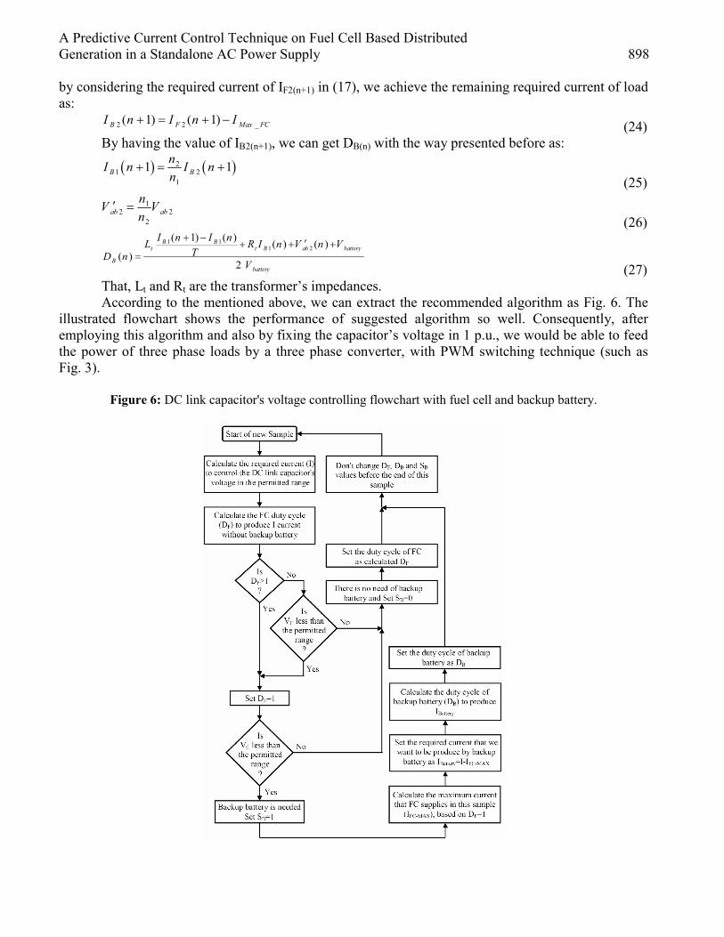
A Predictive Current Control Technique on Fuel Cell Based Distributed Generation in a Standalone AC Power Supply 898 by considering the required current of IF2(n+1) in (17), we achieve the remaining required current of load as:
2 2 _( 1) ( 1)B F Max FCI n I n I+ = + − (24) By having the value of IB2(n+1), we can get DB(n) with the way presented before as:
( ) ( )21 2
1
1 1B BnI n I nn
+ = + (25)
12 2
2ab ab
nV Vn
′ = (26)
1 11 2
( 1) ( ) ( ) ( )( )
2
B Bt t B ab battery
Bbattery
I n I nL R I n V n VTD n
V
+ − ′+ + +=
(27) That, Lt and Rt are the transformer’s impedances. According to the mentioned above, we can extract the recommended algorithm as Fig. 6. The
illustrated flowchart shows the performance of suggested algorithm so well. Consequently, after employing this algorithm and also by fixing the capacitor’s voltage in 1 p.u., we would be able to feed the power of three phase loads by a three phase converter, with PWM switching technique (such as Fig. 3).
Figure 6: DC link capacitor's voltage controlling flowchart with fuel cell and backup battery.

899 K. G. Firouzjah, H. Eshaghtabar, A. Sheikholeslami and S. Lesan
5. Simulation Results In this research, simulations are carried out based on employing the suggested algorithm on adopted system as shown in Fig. 6 and Fig. 1, respectively. MATLAB simulation results show the capability of proposed algorithm to control the switching modes of the fuel cell and backup battery in transient states. Simulations are carried out in the following: 5.1. Fuel Cell's Output Voltage Drops and there is no Backup
In this section, supposed that the boosted output voltage of fuel cell drops below its steady-state value (into 0.5 p.u.). As shown in Fig. 7, FC's voltage dropped and recovered at 0.2 and 1 second respectively. In the other word, a failure occurred during 0.2 through 1 second for the fuel cell. According to Fig. 7, while backup battery is not existed, the DC link capacitor's voltage drops. Also, the voltage and current of three phase load is decreased. 5.2. Fuel Cell's Output Voltage Drops, Load Increases and there is no Backup
We expect that by increasing the load in fuel cell failure the output will have a worse condition than is in section A. Fig. 8 illustrates the verity of this fact. As shown in this figure, a failure occurred during 0.2-1 second for the fuel cell; furthermore the three phase load increased at 0.45 second. These results remark that the output voltage and current have a bad situation in lack of backup battery. 5.3. Fuel Cell's Output Voltage Drops and Backup Battery Exists
In this section, supposed that the boosted output voltage of fuel cell drops below its steady-state value (around 0.5 p.u.) and backup battery is employed based on the proposed algorithm in Fig. 6.
Figure 7: Simulation results under fuel cell's failure and no backup existence.
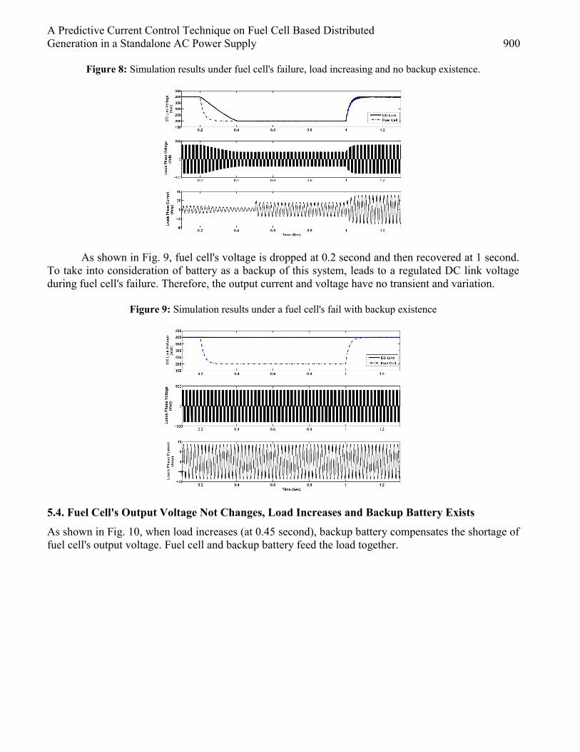
A Predictive Current Control Technique on Fuel Cell Based Distributed Generation in a Standalone AC Power Supply 900
Figure 8: Simulation results under fuel cell's failure, load increasing and no backup existence.
As shown in Fig. 9, fuel cell's voltage is dropped at 0.2 second and then recovered at 1 second. To take into consideration of battery as a backup of this system, leads to a regulated DC link voltage during fuel cell's failure. Therefore, the output current and voltage have no transient and variation.
Figure 9: Simulation results under a fuel cell's fail with backup existence
5.4. Fuel Cell's Output Voltage Not Changes, Load Increases and Backup Battery Exists
As shown in Fig. 10, when load increases (at 0.45 second), backup battery compensates the shortage of fuel cell's output voltage. Fuel cell and backup battery feed the load together.
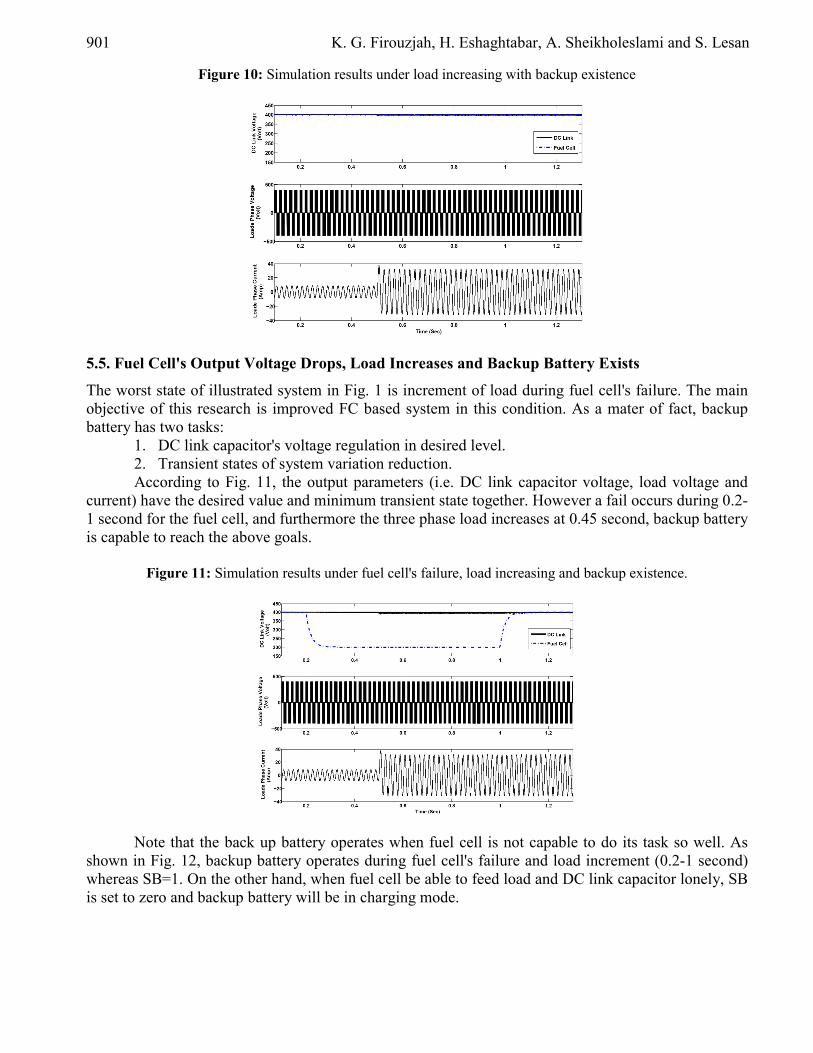
901 K. G. Firouzjah, H. Eshaghtabar, A. Sheikholeslami and S. Lesan
Figure 10: Simulation results under load increasing with backup existence
5.5. Fuel Cell's Output Voltage Drops, Load Increases and Backup Battery Exists
The worst state of illustrated system in Fig. 1 is increment of load during fuel cell's failure. The main objective of this research is improved FC based system in this condition. As a mater of fact, backup battery has two tasks:
1. DC link capacitor's voltage regulation in desired level. 2. Transient states of system variation reduction. According to Fig. 11, the output parameters (i.e. DC link capacitor voltage, load voltage and
current) have the desired value and minimum transient state together. However a fail occurs during 0.2-1 second for the fuel cell, and furthermore the three phase load increases at 0.45 second, backup battery is capable to reach the above goals.
Figure 11: Simulation results under fuel cell's failure, load increasing and backup existence.
Note that the back up battery operates when fuel cell is not capable to do its task so well. As shown in Fig. 12, backup battery operates during fuel cell's failure and load increment (0.2-1 second) whereas SB=1. On the other hand, when fuel cell be able to feed load and DC link capacitor lonely, SB is set to zero and backup battery will be in charging mode.
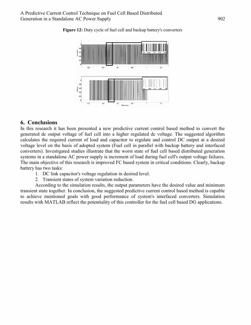
A Predictive Current Control Technique on Fuel Cell Based Distributed Generation in a Standalone AC Power Supply 902
Figure 12: Duty cycle of fuel cell and backup battery's converters
6. Conclusions In this research it has been presented a new predictive current control based method to convert the generated dc output voltage of fuel cell into a higher regulated dc voltage. The suggested algorithm calculates the required current of load and capacitor to regulate and control DC output at a desired voltage level on the basis of adopted system (Fuel cell in parallel with backup battery and interfaced converters). Investigated studies illustrate that the worst state of fuel cell based distributed generation systems in a standalone AC power supply is increment of load during fuel cell's output voltage failures. The main objective of this research is improved FC based system in critical conditions. Clearly, backup battery has two tasks:
1. DC link capacitor's voltage regulation in desired level. 2. Transient states of system variation reduction. According to the simulation results, the output parameters have the desired value and minimum
transient state together. In conclusion, the suggested predictive current control based method is capable to achieve mentioned goals with good performance of system's interfaced converters. Simulation results with MATLAB reflect the potentiality of this controller for the fuel cell based DG applications.

903 K. G. Firouzjah, H. Eshaghtabar, A. Sheikholeslami and S. Lesan
References [1] Akkinapragada, N., 2007. “Dynamic Modeling and Simulations of Solid Oxide Fuel Cells for
Grid-Tied Applications”, Master's Thesis, Electrical Engineering, University of Missouri-Rolla. [2] Anderson, G. K., C. Klumpner, S. B. Kjaer, and F. Blaabjerg, 2002. “A New Power Inverter for
Fuel Cells”, IEEE Conf. Power Electronics Specialists, 2(2), pp. 727-733. [3] Aydemir, M. T., A. Bendre, and G. Venkataramanan, 2002. “A critical evaluation of high
power hard and soft switched isolated DC-DC converters”, IEEE IAS'02, 2, pp. 1338-1345. [4] Bendre, G. Venkataramanan, and D. Divan, 2003. “Dynamic analysis of loss-limited switching
full-bridge DC-DC converter with multimodal control”, IEEE Trans. Industry Applications, 39, pp. 854-863.
[5] Blaabjerg, F., Z. Chen, and S. B. Kjaer, 2004. “Power Electronics as Efficient Interface in Dispersed Power Generation Systems”, IEEE Trans. Power Electronics, 19(5).
[6] Brunoro, M. and J. L. F. Vieira, 1999. “A high-performance ZVS full-bridge DC-DC 0-50-V/0-10-A power supply with phase-shift control”, IEEE Trans. Power Electronics, 14, pp. 495-505.
[7] Chandrasekaran, S., and L. U. Gokdere, 2004. “Integrated Magnetics for Interleaved DC-DC Boost Converter for Fuel Cell Powered Vehicles”, IEEE Conf. PESC 04, 1, pp. 356-361.
[8] Duran-Gomez, J. L., E. Garcia-Cervantes, D. R. Lopez-Flores, P. N. Enjeti, and L. Palma, 2006. “Analysis and Evaluation of a Series-Combined Connected Boost and Buck-Boost DC-DC Converter for Photovoltaic Application”, IEEE Conf. APEC'06, pp. 1-7.
[9] Haiping, X., Q. Ermin, G. Xin, W. Xuhui, and K. Li, 2005. “Analysis and Design of High Power Interleaved Boost Converters for Fuel Cell Distributed Generation System”, IEEE Conf. Power Electronics Specialists, pp. 140–145.
[10] Jain, P. K., Wen Kang, H. Soin, and Youhao Xi, 2002. “Analysis and design considerations of a load and line independent zero voltage switching full bridge DC/DC converter topology”, IEEE Trans. Power Electronics, 17, pp. 649-657.
[11] Jeon, S. -J., and G.-H. Cho, 2001. “A zero voltage and zero-current switching full bridge DC-DC converter with transformer isolation”, IEEE Trans. Power Electronics, 16, pp. 573-580.
[12] Jiang, Z. and R. A. Dougal, 2003. “Control design and testing of a novel fuel-cell-powered battery-charging”, IEEE APEC'03, 2, pp. 1127-1133.
[13] Jung, J. -W., 2005. “Modeling and Control of Fuel Cell Based Distributed Generation Systems”, PhD Dissertation, Ohio State University.
[14] Jung, J. -W., M. Dai, and A. Keyhani, 2005. “Modeling and control of a fuel cell based Z-source converter”, IEEE Conf. APEC 05, 2, pp. 1112-1118.
[15] Keyhani, A. and J. –W. Jung, 2004. “Distributed energy systems”, Journal of Iranian Association of Electrical and Electronics Engineers, 1(2), pp. 33-40.
[16] Kim, E. –S., K. –Y., Joe, M. –H., Kye, Yoon-Ho Kim, and Byung-Do Yoon, 1997. “An improved ZVZCS PWM FB DC/DC converter using energy recovery snubber”, IEEE APEC'97, 2, pp. 1014-1019.
[17] Liu, C., T. Nergaard, L. Leslie, J. Ferrell, X. Huang, T. Shearer, J. Reichl, J. Lai, and J. Bates, 2002. “Power Balance Control and Voltage Conditioning for Fuel Cell Converter with Multiple Sources”, IEEE Conf. Power Electronics Specialists, 4, pp. 2001-2006.
[18] Mohan, N., T. M. Undeland, and W. P. Robbins, “Power Electronics, Converters, Applications and Design”, 2nd Edition, John Wiley & Sons.
[19] Ogura, K., S. Chandhaket, T.Ahmed, and M. Nakaoka, 2003. “Non-Isolated ZVS-PWM Boost Chopper-Fed DC-DC Converter with Auxiliary Edge Resonant Snubber”, IEEE Conf. IECON'03, 3, pp. 2356–2362.
[20] Padulles, J., G. W. Ault, and J. R. McDonald, 2000. “An Approach to the Dynamic Modeling of Fuel Cell Characteristics for Distributed Generation Operation”, IEEE- PES Winter Meeting, 1(1), pp. 134-138.
[21] Peng, F. Z., H. Li, G. –J. Su, and J. S. Lawler, 2004. “A new ZVS bidirectional DC-DC converter for fuel cell and battery application”, IEEE Trans. Power Electronics, 19, pp. 54-65.

A Predictive Current Control Technique on Fuel Cell Based Distributed Generation in a Standalone AC Power Supply 904 [22] Premrudeepreechacharn, S., and T. Poapornsawan, 2000. “Fuzzy Logic Control of Predictive
Current Control for Grid connected Single Phase Inverter”, IEEE Conf. Photovoltaic Specialists Conference, pp. 1715-1718.
[23] Rodriguez, J., J. Pontt, C.A. Silva, P. Correa, P. Lezana, P. Cortes, and U. Ammann, 2007. “Predictive Current Control of a Voltage Source Inverter”, IEEE Trans. Industrial Electronics , 54, pp. 495 – 503.
[24] Rodriguez, J., J. Pontt, C. Silva, P. Cortes, U. Amman, and S. Rees, 2004. “Predictive current control of a voltage source inverter”, Power Electronics Specialists Conference, PESC 04, in Proc. IEEE, 3, pp. 2192 - 2196.
[25] Suzuoka, K., S. Moisseev, L. Gamage, K. Soshin, K. Nishida, and M. Nakaoka, 2003. “Boost Transformer Linked Full Bridge Soft-Commutation DC-DC Power Converter with Secondary-Side Phase-Shifted PWM Rectifier Switches”, IEEE Conf. IECON '03, 1, pp. 49-54.
[26] Wang, C., and M. H. Nehrir, 2006. “Control of PEM Fuel Cell Distributed Generation Systems”, IEEE Trans. Energy Conversion, 21(2), pp. 586-595.
[27] Wang, C., and M. H. Nehrir, 2006. “Short-time Overloading Capability and Distributed Generation Applications of Solid Oxide Fuel Cells”, accepted for IEEE Trans. Energy Conversion.
[28] Wen. X., F. Lin, and T. Q. Zheng, 2006. “Dynamic Model and Predictive Current Control of Voltage Source Converter Based HVDC”, in Proc. IEEE, PowerCon, pp. 1–5.
European Journal of Scientific Research ISSN 1450-216X Vol.20 No.4 (2008), pp.905-913 © EuroJournals Publishing, Inc. 2008 http://www.eurojournals.com/ejsr.htm
Effects of Ethyl acetate Portion of Syzygium Aromaticum
Flower Bud Extract on Indomethacin-Induced Gastric Ulceration and Gastric Secretion
Okasha Mohammad Abdul- Halim Department of Human Physiology, Faculty of Medicine
Ahmadu Bello University, Zaria, Nigeria
Magaji Rabiu Abdussalam Department of Human Physiology, Faculty of Medicine
Bayero University, Kano, Nigeria
Abubakar Mujtaba Suleiman Department of Pharmacognosy and Drug Development, Faculty of Pharmaceutical
Sciences, Ahmadu Bello University, Zaria, Nigeria
Fatihu Muhammad Yakasai Department of Veterinary Pathology and Microbiology, Faculty of Veterinary Medicine
Ahmadu Bello University, Zaria, Nigeria
Abstract
Clove, the dried flower bud of Syzygium aromaticum (Family: Myrtaceae) is one of the important herbs used as indigenous medicine in India, and in Unani Medicine. It contains flavonoids and tannins among others that have bee proven to stimulate the production of prostaglandins which contribute to the maintenance of basal gastric mucosal blood flow and mucus secretion that enhance the mucosal integrity defense and repair of injury. In the present work, we investigated the gastric anti-ulcerogenic and antisecretory effects of the ethyl acetate portion of the ethanolic extract of Syzygium aromaticum (SaETAC) flower bud in rats, using indomethacin as a necrotizing agent. SaETAC demonstrated a gastro-protective anti-ulcerogenic effect as well as a marked decrease of volume, titritable acidity and acid output of gastric secretion in rats. The extract proved to possess some phytochemicals which may contribute to the observed gastric anti-ulcerogenic and anti-secretory activity. Keywords: Syzygium aromaticum, ethyl acetate, indomethacin, gastric ulcer, gastric
secretion 1. Introduction Clove is the dried reddish brown flower bud of Syzygium aromaticum (Family: Myrtaceae), an evergreen tropical tree 10-20 cm in height, indigenous to India, Indonesia, Zanzibar, Mauritius and Sri Lanka. Sometimes, it is called Eugenia caryophyllata. It is one of the important herbs used as
Effects of Ethyl acetate Portion of Syzygium Aromaticum Flower Bud Extract on Indomethacin-Induced Gastric Ulceration and Gastric Secretion 906 indigenous medicine in India, and in Unani Medicine. (Trease and Evans, 1972). It is commonly called “Kanumfari” in Hausa and ‘Kanumfo’ in Yoruba.
Clove is reported as aphrodisiac (Khan, 1893; Tajuddin et al., 2004), stomachic (Nadkarni, 2000; Attar, 1370), carminative, antispasmodic (Khory and Katrak, 1985; Pourgholami et al., 1990). It is also reported to be useful in conceiving in high doses and acts as a contraceptive in low doses (Ibn Al-Baytar, 1869) and useful in cataract (Raazi, 1961).
Peptic ulcers are sores or eroded areas that form in the lining mucosa of the stomach, duodenum, lower esophagus and Merkel’s diverticulum. They affect more than 4 million people each year in the United States (Graham, 1996). Peptic ulcer is the most common gastrointestinal disorder in clinical practice. Oxidative stress and free radical-mediated processes have been implicated in the pathogenesis of gastrointestinal disorders (Salim, 1992).In the absence of non-steroidal anti inflammatory drugs (NSAIDs) use or acid hypersecretory states such as Zollinger-Ellison Syndrome, Helicobacter pylori is the causative factor in 75% of all patients with gastric ulcer and 90% of all patients with duodenal ulcer (Falk, 2000).
Three classes of drugs have been shown to have a direct effect on Helicobacter pylori: antibiotics, bismuth salts, and proton pump inhibitors. Because Helicobacter pylori is difficult to eradicate, most treatment regimens combine agents from two or even all three of these cases. In all of them, patients with active peptic disease should also receive a total of 6 weeks of acid suppression with an H2 receptor antagonist. Peptic ulcer therapy through this combination of drugs has not been very effective due to non-compliance to drugs by patients and possible side effects of the drugs being taken continuously (Peura, 1998).
Considering the several side effects of modern medicine, indigenous drugs with fewer side effects should be looked for as a better alternative for the treatment of peptic ulcer (Salim, 1992). Recent studies found that different substances from plant sources not only afford gastroprotection but also accelerate ulcer healing. They may also possess anti-inflammatory action by suppressing the neutrophil/cytokine cascade in gastrointestinal tract (GIT) (Alarcon de la Lastra et al., 1995), promoting tissue repair though expression of various growth factors, exhibiting antioxidant (Kim et al., 2004) scavenging reactive oxygen species (ROS) (Pastrada-Bonilla et al., 2003; Liu, et al., 2002), showing anti-nucleolytic, cytochrome P450 2F1 inhibitory, anti-necrotic and anti-carcinogenic activities (Bagchi et al., 2002).
There are various plant-originated "gastroprotectors" with different composition that have been used in clinical and folk medicine by many countries due to their beneficial effects on the mucosa of GIT. In China and Japan, polyphenol extracts such as Sopharadin extracts, containing flavonoids and its synthetic flavonoid derivative known as Solon are widely employed in peptic ulcer therapy and also as food additives and nutritional supplements, mainly because of their strong inhibition of prostaglandin (PG) metabolism and vasoconstrictive leukotriene inhibition (Kyogoku et al., 1979).
This study aims at throwing some lights on the effects of ethyl acetate portion of the ethanolic extract of Syzigium aromaticum flower bud on indomethacin-induced gastric mucosal damage and gastric secretion which may help in detection of some gastroprotective properties of this extract. 2. Materials and Methods 2.1. Chemicals and drugs
The following chemicals and drugs were used: Absolute Ethanol (Sigma Aldrich), Ethyl acetate (ETAC) (Sigma Aldrich), Indomethacin (Chiesi) ampoule was used in a dose of 20 mg/kg S.C. as reported by Okabe et al. (1977) and Urushidani et al. (1979). Cimetidine (Lek Pharm. Slovenia) was used in a dose of 50 mg/kg S.C. (Moron et al., 1982) and in a dose of 100 mg/kg S.C. as reported by Satoh et al. (1983), sodium hydroxide (NaOH) (England), phenolphthalein (E.Merck Darmstadt, Germany)

907 Okasha Mohammad Abdul- Halim, Magaji Rabiu Abdussalam, Abubakar Mujtaba Suleiman and Fatihu Muhammad Yakasai
2.2. Preparation of plant material
The flower bud of the Syzygium aromaticum was sourced from ‘Kasuwar Rimi’ market in Kano Metropolis, Nigeria. It was identified and authenticated at the Herbarium section of the Department of Biological Sciences, Ahmadu Bello University and given a voucher number 900132 with deposition of a specimen for further reference. The air dried herb was extracted with aqueous ethanol (70%) in a soxhlet extractor. The extract after concentration at reduced pressure was suspended in methanol and partitioned with ethyl acetate to obtain ethyl acetate (ETAC) portion. The portion was concentrated in vacuum and the residue of the portion was obtained. 2.3. Phytochemical Screening
The extract was screened for the presence of various phytochemicals employing standard screening test (Trease and Evans. 1983). Conventional protocols for detecting the presence of alkaloids, tannins, etc. were used. 2.4. Acute Toxicity Test
LD50 determination was conducted using the method of Lorke (1983). In the first phase male and female mice were divided into three groups of three mice each. After an overnight fasting, the animals were treated with the extract at doses 1000, 100 and 10mg/kg. In the second phase the animals were grouped into four of one mouse each and treated with doses of the extract at 200; 400, 800 and 1600 mg/kg. The animals were observed for 24 hours after treatment and the final LD50 was calculated. 2.5. Animals
Swiss male albino rats ranging in weight from 165- 180 grams were used for this study. The animals were housed under similar conditions of temperature, relative humidity and light/dark cycle with free access to standard laboratory chow and tap water ad libitum. The animals were fasted for 48 hours before the commencement of the experiment with only free access to water (Weisher and Thiemer, 1983). This has been proved to be non-ulcerogenic and sufficient for absolute emptying of the stomach as reported by El-Sokkary et al. (1991). Each of the animals was kept in an individual cage with wide meshed raised floor to prevent coprophagia. The animals were randomly assigned into three different groups:
(1) Indomethacin – treated (control) group (10 rats) Five rats for the study of gastric ulceration and five rats to study gastric secretion.
(2) Extract – treated group (30 rats) Extract (50, 100, &200mg/kg S.C.) was injected 30 minutes before indomethacin to study its effect on gastric secretion and gastric mucosal damage induced by indomethacin.15 rats to study gastric secretion (5rats for each dose) and 15 rats for gastric ulcer studies (5rats for each dose).
(3) Cimetidine – treated (reference) group (20 rats) Cimetidine in a dose of 50 and 100 mg/kg S.C. was used to test its effect on indomethacin – induced gastric ulceration and gastric secretion. Ten rats for gastric secretion studies (5 rats for each dose of cimetidine) and ten rats to study gastric mucosal integrity affection (5 rats for each dose).
2.6. Study of Gastric Ulceration
After the 48 hours fasting, the control group was subcutaneously (S.C.) injected with saline. Experimental groups received SaETAC (50, 100 and 200 mg/kg S.C.) and the reference groups received cimetidine in a dose of 50 and 100 mg/kg B.W. (Moron et al., 1982; Satoh et al., 1983). After

Effects of Ethyl acetate Portion of Syzygium Aromaticum Flower Bud Extract on Indomethacin-Induced Gastric Ulceration and Gastric Secretion 908 30 minutes all the groups were administered indomethacin (20mg/kg S.C.).Then, the animals were deprived of both food and water for seven (7) hours (Urushidani et al., 1979). Later on, the animals were sacrificed by decapitation (Satoh et al., 1983). The stomachs were opened along the greater curvature, rinsed slowly with normal saline then stretched out as much as possible on a Whatman’s filter paper. The ulcerated surface in each stomach was measured with a transparent millimeter scale rule and the result for each group was expressed in mm of mean ulcer ± S.E. (Ulcer index) (Scepovic and Radmanovic, 1984). Preventive index (P.I. %) was later calculated according to the method of Hano et al. (1976) as follows:
U.I. indomethacin – U.I. extract plus indomethacin P.I. % = X 100
U.I. indomethacin 2.7. Study of Gastric Secretion
Gastric juice was collected after making pyloric ligation according to the technique of Shay et al. (1954) as modified by Levine (1965) where esophageal ligation was avoided. The animals were fasted for 48 hours to ensure complete emptying of the stomach, but allowed water ad libitum. The animals were then weighed at the end of the fasting period. Then, under light anaesthesia, the abdomen was opened by midline incision and the stomach was identified. A pyloric ligature was made by using a thread with care to avoid damage of the blood vessels or traction of the stomach. The abdomen was closed by sutures and cleaned thoroughly with saline. The anaesthesia was discontinued and the animals were allowed to recover for a period of three (3) hours. After the 3 hours, the animals were sacrificed and the abdomen of each animal was opened and the esophagus was ligated, then the stomach was removed and washed with saline and dried. An opening along the greater curvature was made and the gastric contents were drained into a graduated centrifuge tube then centrifuged at 3000 rpm for 10 minutes. 2.8. Analysis of the Gastric Juice
2.8.1. Volume of gastric juice After the centrifugation, the supernatant was measured as volume of the gastric juice. 2.8.2. Determination of the Titritable Acidity A given volume of the gastric juice (0.2 ml) was titrated against 0.01 N NaOH using an end point of pH 7.0 as determined colorimetrically with phenol red as an indicator (Grossman, 1963). It was calculated as milliequivalents per liter (mEq/L) which is equal to the number of milliliters (mL) of 0.1 N NaOH required to neutralize 100 ml of the gastric juice
Volume of 0.01N NaOH which neutralizes 1 mL of gastric juice = X 100
10 (Davenport, 1977).
2.8.3. Determination of acid output This was calculated as µEq/h by multiplying the volume of gastric secretion (ml/h) of an animal by the titritable acidity (acid concentration) (mEq/L) of the gastric secretion in that animal (Okabe et al., 1975).

909 Okasha Mohammad Abdul- Halim, Magaji Rabiu Abdussalam, Abubakar Mujtaba Suleiman and Fatihu Muhammad Yakasai
2.9. Statistical Analysis
The experimental data were expressed as the mean ± S.E.M. The significance of the results was determined using analysis of variance (ANOVA) with later comparison by Dunnett’s t-test and the results were considered significant if p < 0.05. 3. Results 3.1. Phytochemical Screening
Preliminary phytochemical analysis of the extract revealed the presence of flavonoids, glycosides, tannins, resins and alkaloids. 3.2. Acute Toxicity Studies
The intraperitoneal LD50 of the extract in mice was found to be 565.7mg/kg. 3.3. Gastric Mucosal Integrity Studies
Indomethacin (20 mg/kg S.C.) produced severe gastric mucosal ulceration restricted to the corpus with an ulcer index of 33.9 ± 1.2. The ulcers appeared in the form of streaks and/or groups and went deep in the mucosa with severe necrotic and hemorrhagic bases.
Administration of SaETAC (100 mg/kg) showed a significant (p<0.05) decrease in the ulcer index (UI) with a preventive index of 52.8%, whereas, SaETAC (200 mg/kg) produced a very highly significant (p<0.001) decrease in the UI (2.6 ± 104) and a preventive index of 92.3% as compared with the control (indomethacin – treated) group. It is also noticed that these marked changes are dose – dependent. Meanwhile, the smaller dose of the extract (50 mg/kg) did not produce any change as shown in table (1).
In regard to Cimetidine, the two dose levels 50 and 100 mg/kg showed an appreciable decrease in the ulcer index which is accompanied by parallel increase in the preventive index (52.2 and 66.1 respectively) as shown in table (1). Table 1: Showing the ulcer index (mm) and the preventive index (%) in the different rat groups.
Indomethacin Extract + indomethacin Cimetidine ± Indomethacin Groups (20mg/kg) (50mg/kg) (100mg/kg) (200mglkg) (50mg/kg) (100mg/kg) Parameters Ulcer index (mean ± S.E.M) 33.9 ± 102 29.0 ± 4.6 16.0 ± 4.8* 2.6 ± 1.4*** 16.2 ± 7.9* 11.5 ± 6.1*
Preventive index 14.5 52.8 92.3 52.2 66.1 Significant variation against Indomethacin – treated group at * = P < 0.05 and *** = P < 0.001 3.4. Gastric Secretion Studies
Administration of SaETAC, in the three dose levels (50,100 & 200 mg/kg), 30 minutes before indomethacin decreased significantly the volume of gastric secretion as compared to indomethacin – treated group. Also, the extract produced a marked decrease in titritable acidity and acid output as related to indomethacin – treated group and the decrease was dose – dependent in both parameters as shown in table (2).

Effects of Ethyl acetate Portion of Syzygium Aromaticum Flower Bud Extract on Indomethacin-Induced Gastric Ulceration and Gastric Secretion 910 Table 2: Showing the different parameters tested on 3 hourly collected gastric secretion for different rat
groups. Indomethacin Extract + indomethacin Cimetidine ± Indomethacin Groups
(20mg/kg) (50mg/kg) (100mg/kg) (200mglkg) (50mg/kg) (100mg/kg) Parameters Volume (ml/3h) 4.14±0.11 2.36±0.34* 2.62±0.25*** 2.20±0.23* 1.30±0.13*** 1.18±0.13***
Titritable acidity(mEq/L) 74.50±1.70 36.44±2.1*** 32.24±1.41*** 18.06±1.41*** 12.8±0.8*** 10.6±0.82***
Acid Output (µEq/h) 102.87±4.0 28.82±4.3*** 27.92±2.4*** 3.25±1.7*** 5.62±0.8*** 4.20±0.6***
Values indicate mean ± S.E.M. Significant variation against Indomethacin – treated group at * = P < 0.05 and *** = P < 0.001
As regards cimetidine, each of the two doses (50 & 100 mg/kg), when administered 30 minutes prior to indomethacin, produced an appreciable decrease in the volume, titritable acidity and acid output of gastric secretion as compared to indomethacin – treated group. It was noticed that the significant changes in all parameters were dose – dependent as shown in table (2). 4. Discussion The gastrointestinal side effects of NSAIDs, especially in the stomach, are one of the most serious complications in patients using these drugs (Hawkey, 2000; Wallace, 1997). Indeed, indomethacin showed potent ulcerogenic action in experimental animals (Takeuchi et al. 1991; Wallace, 1997).
The antiulcerogenic activity of many plant species is related to their content of flavonoids. Spartium junceum L., a species used in Turkish folk medicine to treat gastric ulcer, contains glycosylated flavonoids with antioxidant activity (Yesilada et al., 2000).
There are various plant-originated "gastroprotectors" with different composition that have been used in clinical and folk medicine in many countries due to their beneficial effects on the mucosa of GIT. In China and Japan, polyphenol extracts such as Sopharadin extracts, containing flavonoids and its synthetic flavonoid derivative known as Solon are widely employed in peptic ulcer therapy and also as food additives and nutritional supplements, mainly because of their strong inhibition of prostaglandin (PG) metabolism and vasoconstrictive leukotriene inhibition (Kyogoku et al., 1979).
The phytochemical screening of the plant extract of Syzygium aromaticum carried out by Jenkins et al.(1967), showed that it contains alkaloids, amino acids, flavonoids, proteins, sterols, reducing sugars, tannins and phenols. Another study by Magaji and Yaro (2006) revealed the presence of tannins, resins, steroid glycosides, alkaloids and flavonoids.
Flavonoids have anti-inflammatory activity and protect the gastric mucosa against a variety of ulcerogenic agents in different mammalian species (Harborne and Williams, 2000). As a result, many studies have examined the antiulcerogenic activities of plants containing flavonoids using either naturally derived or synthetic compounds. Plants containing flavonoids were found to be effective in preventing this kind of lesion, mainly because of their antioxidant properties (Cody et al., 1986; Harborne and Williams, 2000).Recently, the antioxidant activity of flavonoids has attracted interest because of the strong evidence that oxidation processes are involved in the mechanisms of several gastric disorders, including ulcerogenesis (La Casa et al., 2000).
The results of the present work revealed that SaETAC extract in the dose level of 100 mg/kg showed a reduction in ulcer index similar to that produced by cimetidine 50 mg/kg and in turn, the preventive index was nearly equal. Meanwhile, the larger dose of the extract (200mg/kg) reported an appreciable decrease in the ulcer index (2.6 ± 1.4) which is much lower than that produced by the big dose of cimetidine (100 mg/kg). Furthermore, both of the extract and cimetidine have reported a significant decrease in the volume and acid output of gastric secretion. Besides, it is noticed that the larger dose of the extract has provided a higher degree of ulcer prevention (92.3%). This gastroprotective effect may be resulting from the marked decrease in the volume and acid output of
911 Okasha Mohammad Abdul- Halim, Magaji Rabiu Abdussalam, Abubakar Mujtaba Suleiman and Fatihu Muhammad Yakasai
gastric secretion produced by administration of the SaETAC extract, in addition to the high flavonoids contained in the extract.
The results of our study are consistent with the results of Giamperi et al. (2004) who reported that grapefruit seed extract showed good gastroprotective antiulcerogenic activity and they attributed this effect to the antioxidative activity of citrus flavonoids found in grapefruit. Also, Heggers and his colleagues (2002) and Reagor et al. (2002) reported that grapefruit flavonoids possess antibacterial, antiviral and antifungal properties.
It can be concluded by the analysis of the obtained data that the anti ulcer activity of SaETAC extract against indomethacin – induced gastric mucosal damage includes: the high content of flavonoids in that extract, its exact mechanism of action remains unclear, but may involve an action on biosynthesis and metabolism of prostaglandins and mucus in the gastric mucosa (Motilva et al., 1994). Also, flavonoids has antibacterial, antiviral, antifungal (Heggers et al., 2002) and antioxidative activity (Giamperi et al., 2004). In addition, the SaETAC extract has decreased the volume and acid output of gastric secretion, as reported from our study results, an effect which may contributes in its gastric mucosal protective activity. References [1] Alarcon de la Lastra, A.C., Martin, M.J., Motilva, V., et al. (1995). Gastroprotection induced by
silymarin, the hepatoprotective principle of Silybum marianum in ischemia-reperfusion mucosal injury: role of neutrophils. Planta Med., 61 (20): 116 – 119.
[2] Attar, H.Z. (1370). Qaranful (clove). In: Ikhtiyarat-e-Badiyee (Persian). Edited by Attar, H.Z. Lucknow, Munshi Nawal Kishore, India, Pp: 381.
[3] Bagchi, D., Ray, S.D., Bagchi, M., Preuss, H.G. and Stohs, S.J. (2002). Mechanistic pathways of antioxidant cytoprotection by a novel IH636 grape seed proanthocyanidin extract. Indian J. Exp. Biol., 40(6): 717-726.
[4] Cody, V., Middleton, E. and Harborne, J. B. (1986). Plant Flavonoids in Biology and Medicine. In: Biochemical, Pharmacological and Structure– Activity Relationships. Alan Liss, New York.
[5] Davenport, H.W. (1977). Gastric secretion. In: Physiology of the Digestive tract. 4th ed. Year Book, Medical Publishers Incorporated, USA, Pp: 102-128.
[6] El-Sokkary, M., Mansour, M.M., El-Ficky, M.S., Okasha, M.A.M., Bacyoni, M., El-Sayed, A.Z. and Abdel-Mottleb, A.M. (1991). Influence of zinc sulphate on gastric ulceration and secretion in indomethacin-treated male rats. J. Biol. Med. Sci. Ther., 7 (1): 366-385.
[7] Falk, P. (2000). Helicobacter pylori - can the mechanisms of pathogenesis guide us towards novel strategies for treatment and prevention? J. Intern. Med., 240: 319-332.
[8] Giamperi, L., Fraternale, D., Bucchini, A., Rocco, D. (2004). Antioxidant activity of Citrus paradise seeds glyceric extract. Fitoterapia, 75(20): 221-224.
[9] Graham, D.Y. (1996). Non-steroidal anti-inflammatory drugs, Helicobacter pylori and Ulcers: where we stand. Am. J. Gastroenterol., 91 (10): 2086.
[10] Grossman, M.I. (1963). Physiology for Physicians. A monthly publication of the American Physiological Society, 1 (7): 1-5.
[11] Hano, J., Bugaski, J., Danek, L., and Wantuch, C. (1976). The effect of neuroleptics on the development of gastric ulcers in rats exposed to restraint and cold stress. Pol. J. Pharmacol. Pharm., 28: 37-47.
[12] Harborne, J. B. and Williams, C. A. (2000). Advances in flavonoid research since 1992. Phytochemistry, 55(6): 481-504.
[13] Hawkey, C.J. (2000). Nonsteroidal anti-inflammatory drug gastropathy. Gastroenterology, 119: 521-535.
Effects of Ethyl acetate Portion of Syzygium Aromaticum Flower Bud Extract on Indomethacin-Induced Gastric Ulceration and Gastric Secretion 912 [14] Heggers, J.P., Cottingham, J., Gusman, J., et al. (2002). The effectiveness of processed
grapefruit seed extract as an antibacterial agent: II. Mechanism of action and in-vitro toxicity. J. Altern. Complement. Med., 8: 333-340.
[15] Ibn Al – Baytar (1869). Qaranful (clove). In: Al Jame’ Li- Mufradat al advia wal Aghzia (Arabic). Volume IV. Edited by: Ibn Al – Batyar. Matba Zahiyah, Zaaherah Mutawaffarah, Cairo, Egypt, Pp: 7-9.
[16] Jenkins, G.L., Knevel, A.M. and Digangi, F.E. (1967). Quantitative Pharmaceutical chemistry. McGraw Hill Book Company, New York, America, Pp: 455-462.
[17] Khan, M.A. (1893). Qaranful (clove). In: Moheet-e-Azam (Persian). Volume III. Edited by: Khan M.A., Matba Nizami, Kanpur, India, Pp: 296.
[18] Khory, R.N., and Katrak, N.N. (1985). Eugenia caryophyllata. In: Materia Medica of India and their therapeutics. Edited by Khory, R.N., Katrak, N.N., Neeraj Publishing House, Delhi, India, Pp: 264-265.
[19] Kim, S.C., Byun, S.H., Yang, C.H., et al. (2004). Cytoprotective effects of Glycyrrhizae radix extract and its active component liquiritigenin against cadmium-induced toxicity (effects on bad translocation and cytochrome c-mediated PARP cleavage). Toxicology, 197(3): 239-251.
[20] Kyogoku, K., Hatayama, K., Yokomori, S., et al. (1979). Anti-ulcer effect of isoprenyl flavonoids. II.Synthesis and anti-ulcer activity of new chalcones related to sophoradin. Chem. Pharm. Bull., 27: 2943-2952.
[21] La Casa, C., Villegas, I., Alarcon de la Lastra, C., Motilva, V. and Calero, M. J. M. (2000).Evidence for protective and anti-oxidant properties of rutine, a natural flavone, against ethanol-induced gastric lesions. Journal of Ethnopharmacology, 71: 45-53.
[22] Levine, R. J. (1965). Stimulation by saliva of gastric secretion in rat. Life Sciences, 4: 959 – 964.
[23] Liu, C.F., Lin, C.C., Lin, M.H., Lin, Y.S. and Lin, S.C. (2002). Cytoprotection by propolis ethanol extract of acute absolute ethanol-induced gastric mucosal lesions. Am. J.Chin. Med., 30(2-3): 245-254.
[24] Lorke, D. (1983). A new approach to practical acute toxicity testing. Arch. Toxicol., 54: 275-287.
[25] Magaji, R.A. and Yaro, A.H. (2006). Preliminary Phytochemical Screening of the Cold Aqueous Extract of Syzygium aromaticum. Biological and Environmental Sciences Journal for the Tropics, 3 (1): 4-6.
[26] Moron, F., Javor, T., Bata, M., Fiegler, M. and Mozsik, G. (1982). The relationship between indomethacin – induced gastric ulcer, ulcer protection by cimetidine and prostacyclin and the cAMP system of the gastric fundic mucosa in the rat. Acta Physiol. Acad. Sci. Hung., 60 (3): 149 – 153.
[27] Motilva, V., Alarcon, de la Lastra, C. and Martin, M.J. (1994). Ulcer-protecting effects of naringenin on gastric lesions induced by ethanol in rat: role of endogenous prostaglandins. J. Pharm. Pharmacol., 46: 91-94.
[28] Nadkarni, K. M. (2000). Myrtus caryophyllus. In: Materia Medica. Edited by: Nadkarni A.K., Popular Prakashan (pvt Ltd), Mumbai, India, Pp: 835-836.
[29] Okabe, S., Honda, K., Takeuchi, K. and Takagi, K. (1975). Inhibitory effect of l-glutamine on gastric irritation and back diffusion of gastric acid in response to aspirin in the rat. Am. J. Dig. Dis., 20 (7): 626-631.
[30] Okabe, S., Takeuchi, K., Urushidani, T., and Takagi, K. (1977). Effects of cimetidine, a histamine H2 – receptor antagonist on various experimental gastric and duodenal ulcers. Am. J. Dig. Dis., 22: 677 – 684.
[31] Pastrada-Bonilla, E., Akoh, C.C., Sellappan, S. and Krewer, G. (2003). Phenolic content and antioxidant capacity of muscadine grapes. J. Agric. Food Chem., 51(18): 5497-5503.

913 Okasha Mohammad Abdul- Halim, Magaji Rabiu Abdussalam, Abubakar Mujtaba Suleiman and Fatihu Muhammad Yakasai
[32] Peura, D. (1998). Helicobacter pylori: Rational Management Options. Am. J. Med., 105: 424 - 430.
[33] Pourgholami, M.H., Kamalinejad, M., Javadi, M., Majzoob, S. and Sayyah, M. (1990). Evaluation of the anticonvulsant activity of the essential oil of Eugenia caryophyllata in male mice. J. Ethnopharmacol., 64: 167-171.
[34] Raazi, A.B.M. (1961). Qaranful (clove). In: Kitab al Haawi Fi al Tibb (Arabic). Volume XXI. Edited by: Raazi A.B.M., Dar al Ma’arif, Hyderabad, India, Pp: 302.
[35] Reagor, L., Gusman, J., McCoy, L., Carino, E. and Heggers, J.P. (2002). The effectiveness of processed grapefruit-seed extract as an antibacterial agent: I. An in vitro agar assay. J. Altern. Complement. Med., 8: 325-332.
[36] Salim, A.W.S. (1992). Use of scavenging oxygen derived free radicals to protect rat against aspirin and ethanol –induced erosive gastritis . J. Pharmaceutical Sci., 81:9.
[37] Satoh, H., Guth, P.H., and Grossman, M.J. (1983). Role of bacteria in gastric ulceration produced by indomethacin in the rat. Cytoprotective action of antibiotics. Gastroenterology, 84: 483-489.
[38] Scepovic, Z. and Radmanovic, B.Z. (1984). Interaction between reserpine and non-steroidal anti-inflammatory drugs in producing gastric ulcers in rats. European J. Pharmacol., 98: 445-448.
[39] Shay, H., Komarov, S., Fells, S.S., Meranz, D., Gruenlein, M. and Siplet, H. (1945). A simple Method for the Uniform production of gastric ulceration in the Rat. Gastroenterology, 5: 43-61.
[40] Tajuddin, A.S., Ahamd, S., Latif, A. and Qasmi, I.A. (2004). Effect of 50% Ethanolic Extract of Syzygium aromaticum (L.) Merr. & Perry (Clove) on Sexual Behaviour of Normal male Rats. Complimentary and Alternative Medicine, 4: 17.
[41] Takeuchi, K., Ueshima, K., Hironaka, Y., Fujioka, Y., Matsumoto, J. and Okabe, S. (1991). Oxygen free radicals and lipid peroxidation in the pathogenesis of gastric mucosal lesions induced by indomethacin in rats. Digestion, 49: 175-184.
[42] Trease, G.E. and Evans, W.C. (1972). Eugenia caryophyllata. In: a Text book of Pharmacognosy. Edited by: Trease, G.E., Evans, W.C., Bailliere Tindall and Cassell, London, England, Pp: 382.
[43] Trease, G. E. and Evans, W. C. (1983). Textbook of Pharmacology. 12th edition. Bailliere Tindall, London, England, Pp: 343 – 383.
[44] Urushidani, T. Kasuya, U. and Okabe S. (1979). The mechanism of aggravation of indomethacin-induced gastric ulcers by adrenalectomy in the rat. Jpn.J. Pharmacol., 29: 775-780.
[45] Wallace, J.L. (1997). Nonsteroidal anti-inflammatory drugs and gastroenteropathy: the second hundred years. Gastroenterology, 112: 1000-1016.
[46] Weischer, C.H. and Thiemer, K. (1983). A method of induction of cold, indomethacin and restraint ulcers in rats. Meth. and Find. Clin. Pharmacol., 5 (5): 315-319.
[47] Yesilada, E., Tsuchiya, K., Takaishi, Y. and Kazuyoshi, K., J. (2000). Isolation and extraction of free radical scavenging flavonoid glycosides from the flowers of Spartium junceum by activity guided fraction. Ethnopharmacology, 73(3): 471-478.

European Journal of Scientific Research ISSN 1450-216X Vol.20 No.4 (2008), pp.914-923 © EuroJournals Publishing, Inc. 2008 http://www.eurojournals.com/ejsr.htm
Real Digital TV Accessed by Cellular Mobile System
Basil M. Kasasbeh Faculty of Information Technology, Applied Science University
Amman 11931, Jordan E-mail: [email protected]
Rafa E. Al-Qutaish
Faculty of Information Technology, Applied Science University Amman 11931, Jordan
E-mail: [email protected]
Muzhir S. Al-Ani Faculty of Information Technology, Amman Arab University
Amman 11953, Jordan E-mail: [email protected]
Khalid Al-Sarayreh
Faculty of Information Technology, Applied Science University Amman 11931, Jordan
E-mail: [email protected]
Abstract
Presently, there is a huge revolution through the use of internet and cellular mobile units, that almost dominant the world by a huge investment in this field. This paper aims at incorporating the digital live TV video to the cellular mobile system. The next generation cellular mobile communication system can have the ability to access the video TV with high resolution. This system is constructed by receiving and multiplexing satellite TV channels to be standby and accessible. Keywords: Wireless Communication, Cellular Networks, Mobile Communication, TV
Broadcast, Next Generation Mobile Systems, Multimedia Systems, Video Transmission.
1. Introduction Marconi’s invention in 1901 led to start new fields of telecommunications revolution such as radio, TV, satellite, mobile, wireless networking and cellular technology. Nowadays, wireless communications and networks play an important part of communications over the world and led a wonderful growth of market [1].
Wireless and cellular revolution is apparent in the growth of the mobile phone market. In 1990 the mobile phone users were approximately 11 millions but this number is increasing rapidly to 1 billion in 2004. The future predicts billions and billions of users and so of investments. This huge

Real Digital TV Accessed by Cellular Mobile System 915
number of users over the world needs a simple, convenient, standard, compatible, flexible, and wide variety of services [2].
Last few years the cost associated with mobile telephones have been decreasing. Mobile telephone prices have dropped since 1996 and they are an economical way to provide phone service to the population. New types of wireless devices are being introduced that have access to the internet to achieve the services available on the internet. Modern mobiles units consist of elegant and comfortable features that lead to new services.
Nowadays, there is a huge revolution through the use of internet and cellular mobile units, that almost dominant the world by a huge investment in this field. This paper aims at incorporating the digital live TV video to the cellular mobile system. The next generation cellular mobile communication system can have the ability to access the video TV with high resolution. This system is constructed by receiving and multiplexing satellite TV channels to be standby and accessible.
This paper presents an overview the digital TV broadcasting in Section 2 and an overview of the digital satellite TV in Section 3. Section 4 discusses the digital video broadcasting. In section 5, the third generation wireless system is discussed. Section 6 describes the next generation wireless system. Section 7 presents the proposed RD-TV-CM system. Finally, a discussion in Section 8 concludes the paper. 2. Digital TV Broadcast Many attempts have been examined to introduce digital TV with higher resolution, but these affect the huge number of existing old systems. One approach to design a common standard for digital broadcasting TV goes in parallel with mobile communications systems applying video compression [3].
In 1993 the aim of development a common digital TV system for Europe were named Digital Video Broadcasting (DVB) and Digital Audio Broadcasting (DAB). The goal of DVB is to introduce digital television broadcasting using satellite transmission and terrestrial transmission. Different levels of quality are integrated in receiver decoder such as [4]:
• Standard Definition TV (SDTV) • Enhanced Definition TV (EDTV). • High Definition TV. • Multimedia PC. • High Resolution Systems (HRS). Transmits data using flexible containers are basically using MPEG-2 frames. DVB sends
service information contained in its data stream which specifies the content of a container. The following contents have been defined:
• Network Information Table (NIT) that lists the services of provider set-top boxes. • Service Description Table (SDT), that lists names and parameters for each service within an
MPEG multiplexed channel. • Event Information Table (EIT) that contains status information about the current
transmission and some additional information for set-top boxes. • Time and Data Table (TDT), that contains update information for set-top boxes. These different types of data are either contains a single channel for HDTV, multiple channels
for EDTV or SDTV, or multimedia data broadcasting [5]. 3. Digital Satellite TV The invention of Satellite led to a big revolution in communications that have been used in the following fields: weather forecasting, Radio & TV broadcasting, military applications and navigation.

916 Basil M. Kasasbeh, Rafa E. Al-Qutaish, Muzhir S. Al-Ani and Khalid Al-Sarayreh
Motion Picture Expert Group (MPEG) describes a form of compression for digital moving images of TV. This format also allows for audio datastreams synchronizing with the video. Analog satellite TV uses around 27-36 MHz of bandwidth for its FM video and FM audio subcarriers for each channel. So the operators put some separate channels, via a digital datastream into a similar bandwidth. The actual compression ratio can be varied with the needs of suppliers of the video information between Studio needs 12 Mbps, Broadcast needs 8 Mbps and VHS needs 2 Mbps [3].
The Digital data from several channels can be multiplexed into an MPEG Transport Stream (MPEG-TS) along with various audio channels. A package with several channels modulated onto one carrier. The lowest compression ratio will occupy the highest bandwidth but will be needed when the video content requires much detail. 4. Digital Video Broadcast Digital Video Broadcast (DVB) is another group that is important and interesting in satellite transmission. DVB or any satellite system must have at least the following features that required for Integrated Receiver Decoder (IRD) (i.e satellite box) [6]: 1. System Recommended Requirements
• MPEG-2 transport stream is used. • Service information is based on MPEG-2 program specific information • Scrambling is defined by CA (Conditional Access) technical group. • CA uses the MPEG-2 CA-descriptor.
2. Video Recommended Requirements:
• MPEG-2 main profile at main level is used (1.5-15 Mbps). • The frame rate is 25 Hz. • Encoded pictures may have either 4:3 or 16:9 aspect ration. • IRDs will support 4:3 and 16:9 aspect ratio. • IRDs must support the use of pan and scan vectors to allow 4:3 monitor to give a full screen
display of 16:9 coded picture. • IRDs must support a full screen display of 720*576 pixels. • IRDs must provide appropriate up conversion to produce a full screen display of 544*576
pixels and 480*576. 3. Audio Recommended Requirements
• MPEG-2 layer I and layer II must be supported by the IRD. • The use of layer II is recommended for the encoded bitstream. • IRDs must support single channel, dual channel joint stereo and extraction of at least a
stereo pair from MPEG-2 compatible multichannel audio. • IRDs must support sampling rates of 32 kHz, 44.1 kHz and 48 kHz.
5. Third Generation Wireless System The objective of the third generation (3G) wireless communications is to provide fairly high speed wireless communications to support multimedia, data, video in addition to voice. The ITU for the year 2000 was developed the IMT-2000 that defined the 3G capabilities as, voice quality, 144 kbps data rate for high speed vehicles, 384 kbps data rate for slowly moving, 2.048 Mbps for office use, symmetrical and asymmetrical data transmission rates, support for both packet switched and circuit switched data
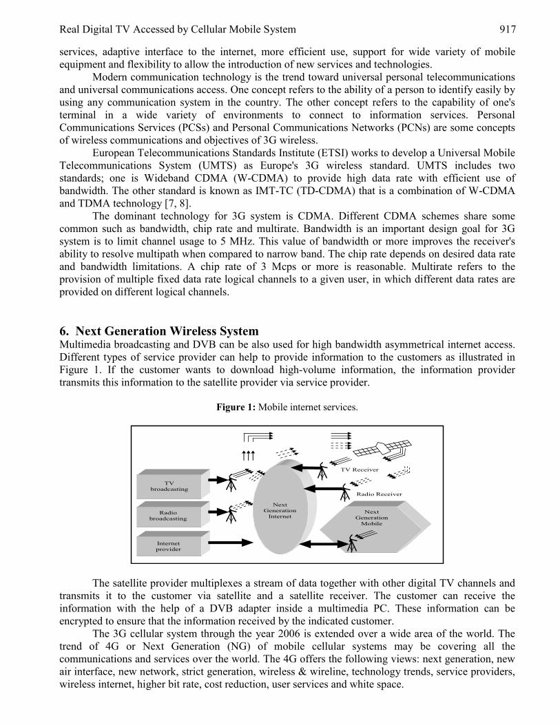
Real Digital TV Accessed by Cellular Mobile System 917
services, adaptive interface to the internet, more efficient use, support for wide variety of mobile equipment and flexibility to allow the introduction of new services and technologies.
Modern communication technology is the trend toward universal personal telecommunications and universal communications access. One concept refers to the ability of a person to identify easily by using any communication system in the country. The other concept refers to the capability of one's terminal in a wide variety of environments to connect to information services. Personal Communications Services (PCSs) and Personal Communications Networks (PCNs) are some concepts of wireless communications and objectives of 3G wireless.
European Telecommunications Standards Institute (ETSI) works to develop a Universal Mobile Telecommunications System (UMTS) as Europe's 3G wireless standard. UMTS includes two standards; one is Wideband CDMA (W-CDMA) to provide high data rate with efficient use of bandwidth. The other standard is known as IMT-TC (TD-CDMA) that is a combination of W-CDMA and TDMA technology [7, 8].
The dominant technology for 3G system is CDMA. Different CDMA schemes share some common such as bandwidth, chip rate and multirate. Bandwidth is an important design goal for 3G system is to limit channel usage to 5 MHz. This value of bandwidth or more improves the receiver's ability to resolve multipath when compared to narrow band. The chip rate depends on desired data rate and bandwidth limitations. A chip rate of 3 Mcps or more is reasonable. Multirate refers to the provision of multiple fixed data rate logical channels to a given user, in which different data rates are provided on different logical channels. 6. Next Generation Wireless System Multimedia broadcasting and DVB can be also used for high bandwidth asymmetrical internet access. Different types of service provider can help to provide information to the customers as illustrated in Figure 1. If the customer wants to download high-volume information, the information provider transmits this information to the satellite provider via service provider.
Figure 1: Mobile internet services.
TV broadcasting
Radio broadcasting
Internet provider
Next Generation
InternetNext
Generation Mobile
TV Receiver
Radio Receiver
The satellite provider multiplexes a stream of data together with other digital TV channels and transmits it to the customer via satellite and a satellite receiver. The customer can receive the information with the help of a DVB adapter inside a multimedia PC. These information can be encrypted to ensure that the information received by the indicated customer.
The 3G cellular system through the year 2006 is extended over a wide area of the world. The trend of 4G or Next Generation (NG) of mobile cellular systems may be covering all the communications and services over the world. The 4G offers the following views: next generation, new air interface, new network, strict generation, wireless & wireline, technology trends, service providers, wireless internet, higher bit rate, cost reduction, user services and white space.

918 Basil M. Kasasbeh, Rafa E. Al-Qutaish, Muzhir S. Al-Ani and Khalid Al-Sarayreh
The trends of NG mobile system may be deployed around the year 2010. The aim is to integrate all type of services in a single frame. NG is not necessary defined by specific features but by significant advance in system capability beyond what can be achieved with 3G. The NG data transmission rate are planned to be up to 20 Mbps, which 10 times faster than the 3G. NG will allow high quality smooth video transmission.
Multimedia network illustrated in Figure 2 to cover a huge number of different types of services that are compatible and accessible to the next generation mobile system. The suggestion of a new technologies supported to computers, communications and networking to standardized and merge all forms of data including audio and video in a multimedia streams. The customer can access any service via its IP address identification. This form can be standardized and any sub network can connect via adapted interface to the high speed internet to form a big and huge collection of services over the world that is the Multimedia Broadcast over a Cellular Network (MBCN). The Fast Information Channel (FIC) is transmitted using a special modulation scheme that is a Multi Carrier Modulation (MCM). The last stage before transmitter is the wide band Orthogonal Frequency Division Multiplexing (OFDM) that is able to compact wide band of information [9].
Figure 2: Multimedia multiplexing system.
Channel Coder n
FastInformation
Channel (FIC)
Audio Service
Audio Encoder
Channel Coder 1
Channel Coder n
Data Service
Packet Encoder
Channel Coder 1
Channel Coder n
VideoService
Video Encoder
Channel Coder 1
Main Service Channel
MSC MUX
Trans-mission MUX OFDM
Transmitter
Transmitted Signal
7. Proposed RD-TV-CM System Nowadays, we are looking for a tremendous revolution in mobile system services and applications. Different types of wireless data transmission that applied cellular technology have unsymmetrical characteristics. In order to integrate these different multimedia systems over a standard network, it must be capable to adapt these different types of data. Many important features must be standardized to reach an integrated of all available system. Wide bandwidth, high bit rate and huge amount of capacity are the most important features to recover all multimedia transmissions as well as some specifications for cellular mobile to store and display the received data.
Introduction of mobile IP address offers a new technology of mobile access to all internet services with some retraction of speed. The digital TV channels can be transmitted via satellite and then received by the customer as requested information.
The consumers, looking for near future, through the introduction of new mobile technologies, so by using these devices they can be able to access all the services over a separate air interface. The

Real Digital TV Accessed by Cellular Mobile System 919
proposed Real Digital TV accessed by Cellular Mobile (RD-TV-CM) may be constructed through eight items; the next subsections describe these eight items. 7.1. Satellite Configuration
Many configurations can be provided between earth station and satellite antenna, and the suitable one is being used to provide point to point link between base station transmitter and Base Station Mobile Center Receiver (BS-MCR) through the satellite as shown in Figure 3.
Figure3: Broadcasting TV satellite.
Satellite 1
Multi Receivers
Multi Receivers Transmitter 1
Satellite 2
Multi Receivers
Multi Receivers
Transmitter 2
7.2. Channels Distribution
The construction of BS-MCR is built to receive several satellite sits from different areas over the world. These multiple receivers are fixed on their specific areas and each sub receiver is concentrated on a number of channels. This is built through a two set of nested multiplexers, one set for satellite and the other for channels as shown in Figure 4.
Figure 4: Multiplexing channel system.
.
.
.
.
.
.
.
.
.
.
.
.
.
.
.
SATm_CHn
Channel Multiplexing
Satellite Multiplexing
SAT1
SATm
SAT1_CH1
SAT1_CHn Selected Channel
7.3. Image Compression
High digital TV image is at least 1024*1024 pixels. So retransmitted this form needed a huge capacity as well as high speed. The aim is to introduce this image in new form to be adapted with the suggested
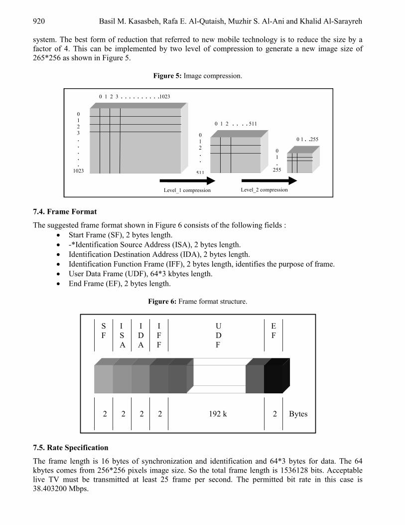
920 Basil M. Kasasbeh, Rafa E. Al-Qutaish, Muzhir S. Al-Ani and Khalid Al-Sarayreh system. The best form of reduction that referred to new mobile technology is to reduce the size by a factor of 4. This can be implemented by two level of compression to generate a new image size of 265*256 as shown in Figure 5.
Figure 5: Image compression.
0 1 .
255
Level_2 compression
0 1 2 . .
511
Level_1 compression
0 1 2 3 . . . . .
1023
0 1 2 3 . . . . . . . . . .1023
0 1 2 . . . . 511
0 1 . .255
7.4. Frame Format
The suggested frame format shown in Figure 6 consists of the following fields : • Start Frame (SF), 2 bytes length. • -*Identification Source Address (ISA), 2 bytes length. • Identification Destination Address (IDA), 2 bytes length. • Identification Function Frame (IFF), 2 bytes length, identifies the purpose of frame. • User Data Frame (UDF), 64*3 kbytes length. • End Frame (EF), 2 bytes length.
Figure 6: Frame format structure.
E F
S F
I F F
I D A
I SA
UDF
2 2 2 2 192 k 2 Bytes
7.5. Rate Specification
The frame length is 16 bytes of synchronization and identification and 64*3 bytes for data. The 64 kbytes comes from 256*256 pixels image size. So the total frame length is 1536128 bits. Acceptable live TV must be transmitted at least 25 frame per second. The permitted bit rate in this case is 38.403200 Mbps.

Real Digital TV Accessed by Cellular Mobile System 921
7.6. Handover
The aim of handover in a Cellular system should not cause a cut-off and keep call in best quality, during the mobility of mobile out of the BTS range or crossing the boundaries of the cell. When a mobile phone access the satellite TV broadcasting, so it must be adapted to any movement of mobile phone as well as the satellite movements. This is done by an Intelligent Supervisory System (ISS) to compare between all the parameters as shown in Figure 7.
Figure 7: Intelligent Handover.
Intelligent Supervisory System
Handover in Satellite System
Handover in Mobile System
7.7. Operation
The company mobile center installed a many receivers to receive a certain satellites. The next generation mobile unit is built to load and excite TV software. The operation started firstly when a mobile user requesting a specific satellite TV, that is confirmed by MSC company. Secondly the mobile user requesting a specific channel, that is also confirmed by MSC. When all the lows are in order, so the requested service has been in the hand of the mobile user as shown in Figure 8.
Figure 8: Transmitting of data.
Ack. Sat.
Req. Ch.
Ack. Ch.
Satellite Center
Mobile Center
MobileUser
Req. Sat.
Data Flow

922 Basil M. Kasasbeh, Rafa E. Al-Qutaish, Muzhir S. Al-Ani and Khalid Al-Sarayreh 7.8. System structure
The structure of the system can be divided into the following five subsystems: 1. Satellite Antenna (SA), 2. Satellite Receiver (SR), 3. Multiplexing System (MS), 4. Mobile Network (MN), and 5. Mobile Subscriber (MS). The MS demand a specific satellite then a certain channel by the software executed over the
mobile phone. These informations transmitted to the MS through the MN. The MS pointed to the indicated satellite and channel and insure a line from the requested channel to the subscriber. 8. Conclusion Currently, there is a huge revolution through the use of internet and cellular mobile units, that almost dominant the world by a huge investment in this field. This paper aims at incorporating the digital live TV video to the cellular mobile system. The next generation cellular mobile communication system can have the ability to access the video TV with high resolution. This system is constructed by receiving and multiplexing satellite TV channels to be standby and accessible.
Huge amount of money invested in the market of Wireless telecommunications networks that leads to new technologies to serve this field. The impaction of all multimedia data in a single channel can be accessed from mobile unit is a strong and power technology which is an elegant face of the next generation mobile system. The system is simple and depends on the multiplexing of different multimedia services that can be accessed by the subscriber. This distribution is flexible and compatible that permits the customer to access any services from its own mobile unites at any site over the world. This system must be intelligent to avoid loaded capacity when a huge number of subscribers need to access the same service. This system can be reach its maximum efficiency, when the next generation well be reachable and accessible with their adaptable high speed of transmission, high verity of services, high capacity of channels, high quality and performance of mobile units with high screen resolution. Acknowledgement This work was supported by the Applied Science University, Amman, Jordan.

Real Digital TV Accessed by Cellular Mobile System 923
References [1] W. H. Al-Sawalmeh and M. S. Al-Ani, “Signal Strength Measurements in GSM”, Asian
Journal of Information Technology, Vol. 3, No. 11, 2004, pp. 1103-1107. [2] W. Stallings, Wireless Communications and Networks, Prentice Hall, New Jersey, 2002. [3] W. X. Wang and S. D. Blostein, “Video Image Transmission over Mobile Satellite Channel”,
Elsevier, Signal Processing (Image Communication), Vol. 16, No. 6, 2001, pp. 531-540. [4] D. E. Comer, Network Systems Deign Using Network Processors, Person Education Inc., 2004. [5] K. B. Benson and D. G. Fink, HDTV Advanced TV, McGraw Hill, New York 1991. [6] J. W. Mark and W. Zhuang, Wireless Communications and Networking, Prentice Education,
New Jersey, 2003. [7] P. M. Heysters, H. Bouma, J. Smit and G. J. M. Smit, “A Reconfigurable Function Array
Architecture for 3G and 4G Wireless Terminals”, in proceedings of the World Wireless Congress, San Francisco, USA, 2002
[8] J. Schiller, Mobile Communications, Person Education Limited, England, second edition, 2003. [9] G. J. M. Smit, P. J. M. Havinga, M. Bos, L. T. Smit and P. M. Heysters, “Reconfiguration in
Mobile Multimedia Systems”, in proceedings of Progress Workshop on Embedded Systems, Utrecht, Netherlands, 2000
European Journal of Scientific Research ISSN 1450-216X Vol.20 No.4 (2008), pp.924-933 © EuroJournals Publishing, Inc. 2008 http://www.eurojournals.com/ejsr.htm
A Rule-Based Fuzzy Automatic Voltage Regulator for
Power System Stability
Samuel N. Ndubisi Department of Electrical and Electronic Engineering, Enugu State University of Science and Technology PMB 01660, Enugu, Nigeria
E-mail: [email protected] Tel.: 2348037046217
Marcel .U. Agu
Department of Electrical Engineering, University of Nigeria Nsukka Enugu State, Nigeria
Abstract
Conventional automatic voltage regulators (CAVR) are observed to have limited operational performance as regards to the control of turbo generator terminal voltage and reactive power during abnormal operating conditions. This is due to its fixed parameters and linearized models of the power system. This paper presents a rule based fuzzy logic controller configured in form of proportional integral controller. It showed a very high improved control of the turbo generator terminal voltage due to very high number of rules (11×11) used and the plant model is not really being considered. Settling time, over shoot etc. were equally reduced by the new controller. Keywords: Conventional automatic voltage regulators; fuzzy logic controller; exciter;
fuzzy rules. 1. Introduction The primary function of the Automatic Voltage Regulator (AVR) of the turbo generator (TG) is to control the terminal voltage and reactive power whilst also ensuring proper sharing of the reactive power amongst parallel connected generators. Load changes and faults always subjects TGs which are nonlinear systems to terminal voltage and reactive power variations. The AVR design must be robust enough to cope with both normal load and fault condition of operation. The resultant effect of all these changes in operating condition is that there will be considerable changes in the TG dynamics. Research has shown that conventional linear fixed gain AVRs can worsen the performance under this condition. Response variations in some circumstances causes negative damping, and degrading system stability [1].
Also the TG model is needed before designing the AVR controller. The idea in this work is to overcome these problems by developing an exact functional replacement for a conventional AVR, with machine voltage the only feedback signal. It is based on the fuzzy logic control.
The fuzzy logic concept incorporates an alternative way which allows one to design a controller using a higher level of abstraction without knowing the plant model [2]. This makes fuzzy logic controllers very attractive for ill defined systems with uncertain parameters. With the help of fuzzy

A Rule-Based Fuzzy Automatic Voltage Regulator for Power System Stability 925
logic concepts, experts’ knowledge can be used directly to design a controller. Fuzzy logic allows one to express the knowledge with subjective concepts such as very big, too small, moderate and slighty deviated, which are mapped to numeric ranges [3].
Fuzzy control implementation of AVR has been reported in a number of publications [4,5,6]. Due to its lower computation burden and its ability to accommodate uncertainties in the plant model, fuzzy logic PI configured AVR (FAVR) appear to be suitable for implementing AVRs. The implementation of FAVR is through simple microcomputer with A/D and D/A converters [7]. The performance of this controller is observed to depend on the operating conditions of the system, although, it is less sensitive than conventional linear PI controller. In this paper, a rule based fuzzy logic PI configured controller is developed for excitation and generator terminal voltage control. The vast rule (11×11) developed for the FAVR made it well suitable for different operating conditions of the plant. The controller is applied to a mathematical model of the exciter and synchronous generator. The responses of the machine subject to a fault in the transmission line is obtained by nonlinear simulations [7]. System responses for three different operating conditions are conducted using FAVR, conventional PI, and PID controller. All the simulations are carried out using MATLAB software package. Result shows reduction in overshoot, settling time, rise time and overall responses. 2. Rule – Based Fuzzy Logic AVR A fuzzy logic controller (FLC) is a special kind of a state variable controller governed by a family of rules and a fuzzy inference mechanism. The FLC algorithm can be implemented using heuristic strategies, defined by linguistically described statements. The fuzzy logic control algorithm reflects the mechanism of control implemented by people, without using any formalized knowledge about the controlled plant in the form of mathematical models, and without an analytical description of the control algorithm. The main FLC are fuzzification, rule base, inference mechanism and defuzzification [8]. Fuzzification is the process of transferring the crisp input variables to corresponding fuzzy variables. In this work, the error between the desired voltage Vd and the terminal voltage Vt i.e. Ve and the integral of the error VI are the two inputs. Ve is fuzzified according to the membership functions shown in fig.1 and is similar to membership function of VI.
For each input variable eleven labels are defined, namely: NV, NL, NB, NM, NS, ZR, PS, PM, PB, PL and PV which stands for negative very large, negative large, negative big, negative medium, negative small, zero, positive small, positive medium, positive big, positive large and positive very large. This numerically stands for (-1, -0.8, -0.6, -0.4, -0.2, 0, 0.2, 0.4, 0.6, 08 and 1). With the two inputs for this FLC, an (11×11) decision table is constructed as shown in Table 1. Every entity in the table represents a rule. The antecedent of each rule conjuncts Ve and VI fuzzy set values. An example of the ith rule is: if Ve is NS and VI is PL then U is PB. This means that if the voltage error is negative small and integral of voltage error is positive large then the output of controller should be positive big.
Figure 1: Membership functions for input Ve
The procedure for calculating the crisp output of the FLC for some values of input variables is based on the following three steps [8];

926 Samuel N. Ndubisi and Marcel .U. Agu
STEP 1: Determination of the degree of firing (DOF) of the rules
The (DOF) of the ith rule consequent is a scalar value which equals the minimum of the two antecedent membership degrees. Table 1: Decision table of 121 rules
Integral of voltage error VI Voltage error Ve NV NL NB NM NS ZR PS PM PB PL PV NV NV NV NV NV NV NV NL NB NM NS ZR NL NV NV NV NV NV NL NB NM NS ZR PS NB NV NV NV NV NL NB NM NS ZR PS PM NM NV NV NV NL NB NM NS ZR PS PM PB NS NV NV NL NB NM NS ZR PS PM PB PL ZR NV NL NB NM NS ZR PS PM PB PL PV PS NL NB NM NS ZR PS PM PB PL PV PV PM NB NM NS ZR PS PM PB PL PV PV PV PB NM NS ZR PS PM PB PL PV PV PV PV PL NS ZR PS PM PB PL PV PV PV PV PV PV ZR PS PM PB PL PV PV PV PV PV PV
For instance, if Ve is PM with a membership degree of 0.4 and VI is PS with a membership
degree of 0.2 then the degree of firing of this rule is 0.2. STEP 2: Inference mechanism
The inference mechanism consists of two processes called fuzzy implication and rule aggregation. The degree of firing of rule interacts with its consequent to provide the output of the rule, which is a fuzzy subset. The formulation used to determine how the DOF and the consequent fuzzy set interact to form the rule output is called a fuzzy implication. In fuzzy logic control the most commonly used method for inferring the rule output is mamdani method [9, 10, 11]. STEP 3: Defuzzification
To obtain a crisp output value from the fuzzy set obtained in the previous step, a mechanism called defuzzification is used. In this work output u is defuzzified according to the membership functions shown in fig 2. Centre of area method [7] is used for defuzzification.
Figure 2: Membership functions for output u
Tuning: To achieve a fast response from the controller during faults, the FLC can be tunned with the parameters g0, g1 and g2 as shown in fig 4. 3. A Power System Dynamic Model In this paper, simplified dynamic model of a single-machine infinite bus power system is considered [12]. This model consists of a single synchronous machine connected through a parallel transmission

A Rule-Based Fuzzy Automatic Voltage Regulator for Power System Stability 927
line to a very large network approximated by an infinite bus. The classical third order single–axis dynamic model of the simple machine infinite bus power system shown in fig 3 has the equations as follows [12,13] 3.1. Mechanical equations
( ) ( ) 0 - ωωδ tt =& (1)
( ) ( )( ) ( )me PtPH
tHDt −−= )(
2 - 0
0ωωωω&
(2) The mechanical input power Pm is assumed to be constant in the excitation controller design.
This implies that the governor action is slow enough not to have any significant impact on the machine dynamics. 3.2. Electrical generator dynamics
( ) ( ) ( )( )tEtET
tE qfd
q −′
=′ 1 0 (3)
3.3. Electrical equations (assumed qd XX =′ )
( ) ( ) ( ) ( )tIXXtE tE dddqq ′−+′= (4) ( ) ( )tU KtE fcf =′ (5)
( ) ( ) ( )ds
sde X
tVtEtP′
′=
δsin (6)
( ) ( ) ( )ds
sqd X
tVtEtI
′−′
=δcos
(7)
( ) ( )ds
sq X
tVtI
′=
δsin
(8)
( ) ( ) ( )ds
s
ds
sq
XV
XtVtE
tQ′
−′
′=
2cosδ
(9) ( ) ( )tIXtE fad=′ (10)
( ) ( ) ( )( ) ( )( )[ ] 2122 tIXtIXtEtV qdddqt +′−′= (11)
More details of the modeling can be seen in [14]. The definitions of the parameters are as indicated under symbols and abbreviations.
LTdds XXXX ++= (12)
LTdds XXXX ++′=′ (13)
LTs XXX +=

928 Samuel N. Ndubisi and Marcel .U. Agu
Figure 3: A single machine infinite bus power system.
3.4. Linear model of SMIB
By linearizing the above equations about the operating point, we have the state variable model of a single machine to infinite bus (SMIB) as follows
UX BAX +=& (14) CXy = (15)
Where the state variable x is defined by [ ]qEX ′∆∆∆= ,, ωδ (16)
In the above system matrix A, B, and C are represented by
( ) ( )00000
00
11 0 sin
sin2
2
cos
2
0 1 0
⎥⎥⎥⎥⎥⎥⎥⎥
⎦
⎤
⎢⎢⎢⎢⎢⎢⎢⎢
⎣
⎡
′′′−
′−
′′′−
−
′−−
′′
−=
dd
dd
dds
s
d
dd
ds
s
ds
s
XTXX
TXV
TXX
XV
HHD
XqEV
HA
δ
δωδω
⎥⎥⎥⎥⎥⎥
⎦
⎤
⎢⎢⎢⎢⎢⎢
⎣
⎡
′
=
0
0 0
d
c
TK
B
( ) ( ) ( ) ( )
0
2
-1 0 cossin
⎥⎥⎦
⎤
⎢⎢⎣
⎡⎟⎟⎠
⎞⎜⎜⎝
⎛′′′−′
⎟⎟⎠
⎞⎜⎜⎝
⎛′
′+
′′−−′
=ds
d
t
ddq
ds
s
t
qd
ds
sd
t
ddq
XX
VIXE
XV
VIX
XVX
VIXE
C δδ
where sub index 0 shows that matrices are calculated at operating point. 3.5. Simplified voltage and reactive power control loop model (AVR)
It is observed from [15] that in an interconnected power system, that the control is made up of load frequency control loop (LFC) and automatic voltage control loop (AVR). The LFC loop controls changes in real power due to changes in rotor angle while the AVR loop controls the changes in reactive power which depends on excitation voltage magnitude. Because the excitation time constant is much smaller than the prime mover time constant, its transient decay much faster. For this, the cross-compiling between the LFC loop and AVR loop is negligible and hence the load frequency and excitation voltage control can be analyzed independently (see fig 4).
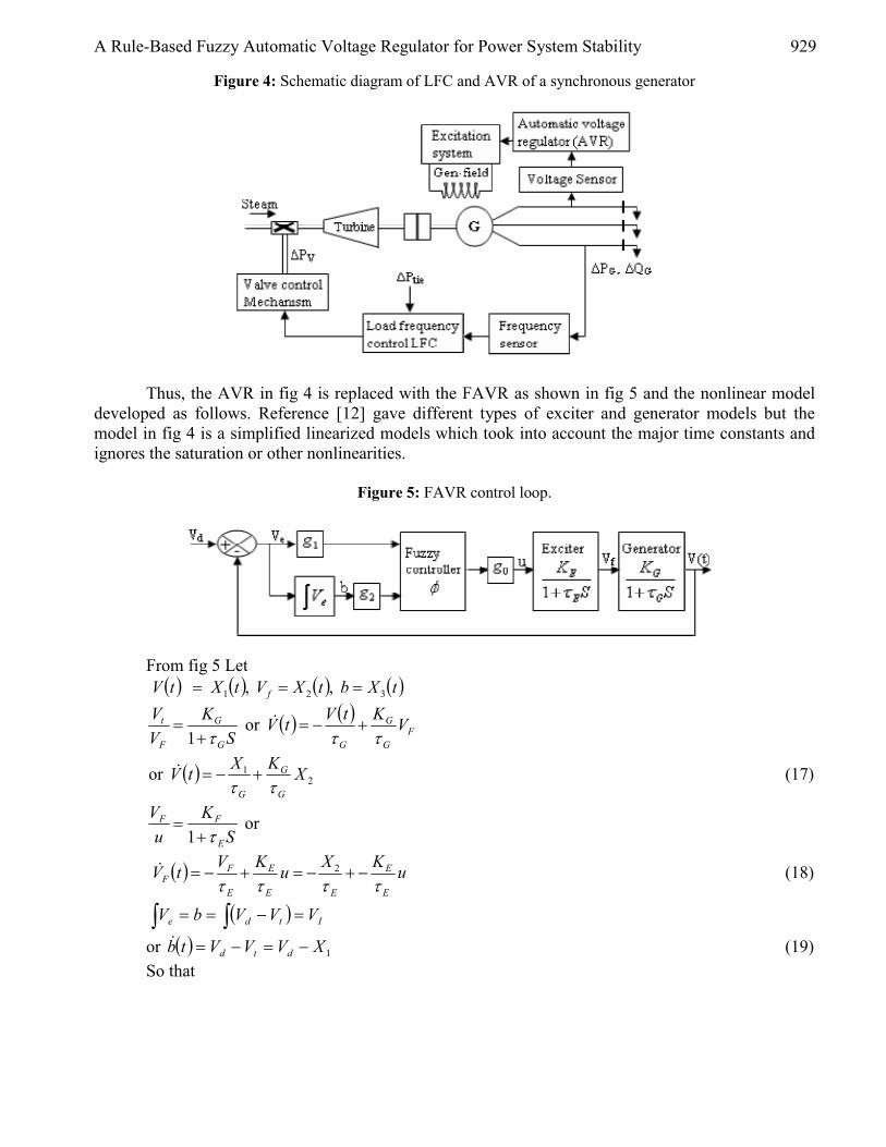
A Rule-Based Fuzzy Automatic Voltage Regulator for Power System Stability 929
Figure 4: Schematic diagram of LFC and AVR of a synchronous generator
Thus, the AVR in fig 4 is replaced with the FAVR as shown in fig 5 and the nonlinear model developed as follows. Reference [12] gave different types of exciter and generator models but the model in fig 4 is a simplified linearized models which took into account the major time constants and ignores the saturation or other nonlinearities.
Figure 5: FAVR control loop.
From fig 5 Let ( ) ( ) ( ) ( )tXbtXVtXtV f 321 , , ===
( ) ( )F
G
G
GG
G
F
t VKtVtVS
KVV
τττ+−=
+= &or
1
( ) 21or XKXtV
G
G
G ττ+−=& (17)
SK
uV
E
FF
τ+=
1 or
( ) uKXuKVtVE
E
EE
E
E
FF ττττ
−+−=+−= 2 & (18)
( ) Itde VVVbV =−== ∫∫
or ( ) 1XVVVtb dtd −=−=& (19) So that

930 Samuel N. Ndubisi and Marcel .U. Agu
( )d
E
E
E
G
G
G
F
t
VuK
K
X
X
X
tb
V
V
F⎥⎥⎥
⎦
⎤
⎢⎢⎢
⎣
⎡+
⎥⎥⎥⎥⎥⎥⎥
⎦
⎤
⎢⎢⎢⎢⎢⎢⎢
⎣
⎡
−
+−
−
=⎥⎥⎥
⎦
⎤
⎢⎢⎢
⎣
⎡
=⎥⎥⎥
⎦
⎤
⎢⎢⎢
⎣
⎡
=100
0 0 1
0 1 0
0 1
3
2
1
ττ
ττ
&
&
&
&
&
&
(20)
( ) ( ) ( ) ;)1()( );(21 ;211⎥⎦
⎤⎢⎣
⎡−×+×−×+×−= XindexVindexu
KXX
KXF d
E
E
EG
G
G ττττ
CXy = (21) 4. Simulation Results The performance of the FAVR controller is examined through simulation using MATLAB software package developed based on the exciter and generator models of fig.5.
It is worth noting that the FAVR here considers only the deviations of the terminal voltage for its set point and the liveliness of the control signal. However, during major disturbances the rotor angle of the generator with respect to the infinite busbar of the power system is disturbed significantly and can take sometime to settle down following the event. It is known that conventional AVR (CAVR) controller can reduce the damping torque of the generator if it uses only the terminal voltage as its feedback signal resulting to reduction of damping of rotor oscillations. This has to be examined sufficiently in a later work.
Two set of tests are carried out A. Voltage v Sudden terminal ariation With this sudden terminal voltage change, four tests were carried out
1. With CAVR, the amplifier transfer function is given by
SK
A
A
τ+1 (22)
and 4.0 ,1 ,1.0 10 ==== EEAA Kτ,K τ , 05.0 ,1 ,1.0 1 ==== RRGG Kτ,K τ has the response shown below.
Figure 6: Terminal voltage step response for CAVR.
2. A stabilizer is connected between the exciter output and the input summer with a step input signal. The stabilizer transfer function is
104.02
+SS (23)

A Rule-Based Fuzzy Automatic Voltage Regulator for Power System Stability 931
The response is shown below with its time domain specifications
Figure 7: Terminal Voltage step response of CAVR with stabilizer
3. A PID is connected in series with the amplifier. The PID parameters are 28.0 and 25.0 ,10 === DIP KKK .
Figure 8: Terminal voltage step response with PID controller.
4. With the FAVR of fig 4, the response to a step input is shown below with the time specifications.
Figure 9: (a) Terminal and desired voltage step response with FAVR
(b) Fuzzy input voltage to the generator

932 Samuel N. Ndubisi and Marcel .U. Agu
B. A Three phase fault was applied after 2 seconds and cleared in 4 seconds in fig 4 and the response of the FAVR is recorded below.
Figure 10: (a) Step response of FAVR to three phase fault.
(b) Fuzzy input voltage to the generator
5. Conclusion A proportional integral (PI) type fuzzy regulator for terminal voltage and reactive power control of turbo generators is considered in this work. The result shows that the FAVR performance is very high as compared to convectional AVR. The overshoot, settling time and rise time are highly reduced during the two tests conducted. The observed set back is on the steady state error which can be cleared by automatically tuning the gains g0, g1 and g2 to achieve the required result. 6. List of Symbols and Abbreviations Symbols
( )tδ power angle of the generator, radian. ( )tω rotor speed of the generator, radian/s
mP mechanical power, p.u. ( )tPe active electrical power delivered by the generator, p.u. ( )tEq′ transient EMF in the quadratic axis in the generator, p.u. ( )tE f equivalent EMF in the excitation coil, p.u. ( )tVt generator terminal voltage, p.u.
sV infinite bus voltage, p.u.
fU output of the PI fuzzy controller. H inertia constant
eV error voltage
dV setpoint or reference voltage
fV exciter output voltage
EK exciter gain
GK generator model gain
Eτ exciter time constant
Gτ generator time constant
021 ,, ggg fuzzy gains

A Rule-Based Fuzzy Automatic Voltage Regulator for Power System Stability 933
Abbreviations
AVR automatic voltage regulator LFC load frequency control FLC fuzzy logic controller FAVR fuzzy automatic voltage regulator CAVR conventional automatic voltage regulator SMIB single machine infinite bus PI proportional and integral controller PID proportional, integral and derivative controller
Acknowledgement This work was supported by the Power Holdings Company of Nigeria (PHCN), Enugu Distribution Zone. References [1] Hogg B.W, “Representation and control of turbo generators in electric power systems,” Chapter
5 in modeling of dynamical systems vol 2: PP 112 - 149 1981. [2] Zadeh L.A “Outline of a new approach to the analysis of complex systems and decision
processes,” IEEE Trans. on systems, man and cybernetics, Vol 3, no 1, 1973, PP 28 - 44 [3] Hassan M.A.M, Malik O.P and Hope G.S, “A fuzzy logic based stabilizer for a synchronous
machine,” IEEE Trans. on Energy conversion, vol. 6, no 3, 1991 PP 407- 413. [4] Weng J.Y, Cheng S.J., Malik O.P. “A Synchronous generator fuzzy excitation controller
optimally designed with a genetic algorithm” IEEE Trans on power systems vol 13, no3, PP 884 884 – 889, August 1998.
[5] Hassan A.R, Sadrul Ula A.H.M “Design and implementation of a fuzzy controller Based Automatic Voltage Regulator for a Synchronous Generator.” IEEE Trans. on Energy conversion, Vol 9, No 3, September 1994.
[6] El-Metwally K.A, and Malik O.P, “Fuzzy logic power system stabilizer.” IEE proceedings on Generation, Transmission and Distribution Vol 142, no 3, May 1995, PP 277 – 281.
[7] Passion K.M and Yurkovich S. “Fuzzy control” Addison Wesley Longman, Inc 1998 [8] Tsoukalas L.H. and Uhrig R.E “Fuzzy and Neural Approach in Engineering.” John Wiley &
Sons, Inc 1997 [9] Mamdani E.H and Assilian S., “An experiment in linguistic synthesis with a fuzzy logic
controller” International Journal of man - machine studies, vol 7, 1975, PP 1-13. [10] Mamdani E.H; “Advances in the linguistic synthesis of fuzzy controllers,” International Journal
of man - machine studies, vol 8, 1976, PP 669-678. [11] Mamdani E.H, Ostergaard J.J and Lambessis E., “Use of fuzzy logic for implementing rule-
base control of industrial processes” Fuzzy sets and Decision Analysis, North Holland: Amsterdam, 1984, PP 429-445
[12] Kundur P, “Power system stability and control,” Mc Graw-Hill, Inc NY 1994. [13] Wang Y, Hill D. J, Middleton R.H and Gao L. “Transient stability Enhancement and voltage
Regulation for power systems,” IEEE Trans on Power systems, vol 8, PP 620-627, 1993 [14] Guo Y., Hill D.J. and Wary Y, “Global Transient stability and voltage Regulation for power
systems” IEEE Transaction on power systems. Vol 16, No 4, PP 678-688, 2001.