LETTERSPUBLISHED ONLINE: 2 SEPTEMBER 2012 | DOI: 10.1038/NCLIMATE1682

Robust projections of combined humidity andtemperature extremesE. M. Fischer* and R. Knutti

Impacts of climate change such as the effects on humandiscomfort, morbidity and mortality often depend on multipleclimate variables. Thus, a comprehensive impact assessmentis challenging and uncertainties in all contributing variablesneed to be taken into account. Here we show that uncertaintiesin some impact-relevant metrics such as extremes of healthindicators are substantially smaller than generally anticipated.Models that project greater warming also show a strongerreduction in relative humidity. This joint behaviour of un-certainties is particularly pronounced in mid-continental landregions of the subtropics and mid-latitudes where the greatestchanges in heat extremes are expected. The uncertainties inhealth-related metrics combining temperature and humidityare much smaller than if uncertainties in the two variables wereindependent. Such relationships also exist under present-dayconditions where the effect of model biases in temperatureand relative humidity largely cancel for combined quantities.Our results are consistent with thermodynamic first principles.More generally, the findings reveal a large potential for jointassessment of projection uncertainties in different variablesused in impact studies.

During recent major summer heatwaves, such as in 2003 incentral and western Europe and 2010 in Russia, themortality locallyincreased by tens of thousands of additional casualties1. Apart fromexcessive temperature anomalies, other factors such as humidity,radiation, lowwinds and air pollution potentially contributed to theenhanced mortality and more generally to the human discomfort.Likewise,many other socio-economic or ecological climate impacts,for example on agricultural production, forest fires, glacier retreat,river runoff or energy production, depend on more than oneclimate variable. Consequently, for a comprehensive assessment ofclimate change impacts it is imperative to take into account theuncertainties in all contributing variables.

In many cases the different climate variables are linked throughfirst principles or basic mechanisms that are well understood, forexample, warmer air being able to hold more moisture, or soilmoisture variations affecting the partitioning of sensible and latentheat. The relationships depend on the temporal resolution of thevariables considered and may vary across different quantiles2,3. Inmany cases they have been found to be relatively well captured bymodels, for example, for temperature and precipitation4,5. Despitethe knowledge about the relationships across variables, they areoften ignored in the context of projections. The Fourth AssessmentReport of the Intergovernmental Panel on Climate Change6, forexample, provides projections of many variables, but each of thoseis discussed separately. Recently some studies have quantifiedhow relationships across variables evolve into the future7,8 orhow their often correlated uncertainties can be transformed into

Institute for Atmospheric and Climate Science, ETH Zurich, Universitätstrasse 16, 8092 Zurich, Switzerland. *e-mail: erich.fischer@env.ethz.ch.

joint probabilistic projections9,10. However, there is a serious lackof research addressing joint projections in variables other thantemperature and precipitation.

Here we use simulations from 15 general circulation models(GCMs; Supplementary Table S1) of the new Climate Model Inter-comparison Project phase 5 (CMIP5; ref. 11) to demonstrate that inselected cases uncertainties in impact-relevant variables are smallerthan generally anticipated. To this end, we focus on two variablesthat are considered as well-established risk factors for humanhealth: temperature and humidity. High ambient temperatures andhumidity reduce the human body’s efficiency of transporting awaythe metabolic heat through evaporative cooling (sweating) andheat conduction12. Consequently, they lead to heat stress and canincrease both morbidity and mortality13. To quantify the combinedeffects of temperature and humidity we here use the simplifiedwet-bulb globe temperature (W ; refs 12,14,15) and the thermody-namicallymotivated equivalent temperature16,17 (seeMethods).

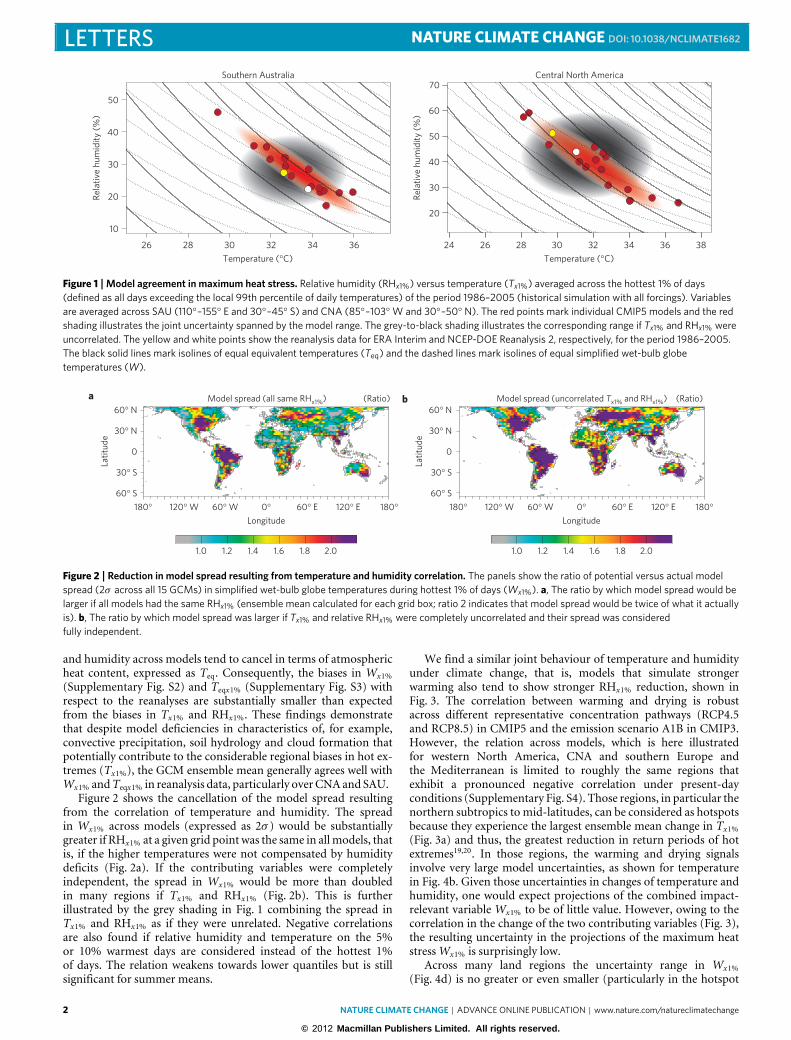
Figure 1 illustrates the 2m temperatures and relative humidityon the 1% warmest days (hereafter, Tx1% and RHx1%) of theperiod 1986–2005 for each GCM (red dots). In both SouthernAustralia (SAU) and Central North America (CNA), present-dayTx1% and RHx1% vary strongly across models (SAU, Tx1%: 29–36 ◦C,RHx1%: 17–46%; CNA, Tx1%: 28–37 ◦C, RHx1%: 24–59%). Thecorresponding values derived from the European Centre forMedium-Range Weather Forecasts (ECMWF) Reanalysis (ERA)Interim (Fig. 1, yellow dots) andNational Centers for Environmen-tal Prediction—Department of Energy (NCEP-DOE) Reanalysis 2(Fig. 1, white dots; see Methods) fall within the range of GCMs.To illustrate the model spread we fit a kernel density estimate18to the bivariate distribution (Fig. 1, red shading). Given thelimited number of models the kernel density should be interpretedwith caution. However, it is evident that models showing hottertemperatures tend to simulate lower relative humidity. Despite thelarge spread in the contributing variables, models agree remarkablywell onW on the hottest 1% of days (Wx1%, solid black lines markequal W levels) and the model spread in Wx1% is substantiallysmaller than if the inter-model differences in the two variableswere uncorrelated (Fig. 1 grey shading). The reduction of modelspread is even more pronounced for equivalent temperature (Teq,that is, the temperature an air parcel would have if all watervapour were condensed; see Methods), which demonstrates thatthe result is consistent with thermodynamical first principles. Theagreement between models and cancellation of model differencesis a consequence of the negative correlation between RHx1% andTx1%. This negative correlation is limitedmainly tomid-continentalland regions in North America, Eurasia, the Amazonian basin andparts of Australia (Supplementary Fig. S1). In these regions therelationship implies that the pronounced differences in temperature

NATURE CLIMATE CHANGE | ADVANCE ONLINE PUBLICATION | www.nature.com/natureclimatechange 1

© 2012 Macmillan Publishers Limited. All rights reserved.

LETTERS NATURE CLIMATE CHANGE DOI: 10.1038/NCLIMATE1682

20

30

40

50

60

70

Rela

tive

hum

idity

(%

)

10

20

30

40

50Re

lativ

e hu

mid

ity (

%)

24 26 28 30 32 34 36 38

Temperature (°C)

26 28 30 32 34 36

Temperature (°C)

Southern Australia Central North America

Figure 1 | Model agreement in maximum heat stress. Relative humidity (RHx1%) versus temperature (Tx1%) averaged across the hottest 1% of days(defined as all days exceeding the local 99th percentile of daily temperatures) of the period 1986–2005 (historical simulation with all forcings). Variablesare averaged across SAU (110◦–155◦ E and 30◦–45◦ S) and CNA (85◦–103◦W and 30◦–50◦ N). The red points mark individual CMIP5 models and the redshading illustrates the joint uncertainty spanned by the model range. The grey-to-black shading illustrates the corresponding range if Tx1% and RHx1% wereuncorrelated. The yellow and white points show the reanalysis data for ERA Interim and NCEP-DOE Reanalysis 2, respectively, for the period 1986–2005.The black solid lines mark isolines of equal equivalent temperatures (Teq) and the dashed lines mark isolines of equal simplified wet-bulb globetemperatures (W).

Model spread (all same RHx1%) Model spread (uncorrelated Tx1% and RHx1%)

60° S

180° 120° W 60° W 0°Longitude

60° E 120° E 180° 180° 120° W 60° W 0°Longitude

60° E 120° E 180°

30° S

0

Latit

ude

Latit

ude

30° N

60° N(Ratio) (Ratio)a

60° S

30° S

0

30° N

60° Nb

1.0 1.2 1.4 1.6 1.8 2.0 1.0 1.2 1.4 1.6 1.8 2.0

Figure 2 | Reduction in model spread resulting from temperature and humidity correlation. The panels show the ratio of potential versus actual modelspread (2σ across all 15 GCMs) in simplified wet-bulb globe temperatures during hottest 1% of days (Wx1%). a, The ratio by which model spread would belarger if all models had the same RHx1% (ensemble mean calculated for each grid box; ratio 2 indicates that model spread would be twice of what it actuallyis). b, The ratio by which model spread was larger if Tx1% and relative RHx1% were completely uncorrelated and their spread was consideredfully independent.

and humidity across models tend to cancel in terms of atmosphericheat content, expressed as Teq. Consequently, the biases in Wx1%(Supplementary Fig. S2) and Teqx1% (Supplementary Fig. S3) withrespect to the reanalyses are substantially smaller than expectedfrom the biases in Tx1% and RHx1%. These findings demonstratethat despite model deficiencies in characteristics of, for example,convective precipitation, soil hydrology and cloud formation thatpotentially contribute to the considerable regional biases in hot ex-tremes (Tx1%), the GCM ensemble mean generally agrees well withWx1% andTeqx1% in reanalysis data, particularly overCNAand SAU.

Figure 2 shows the cancellation of the model spread resultingfrom the correlation of temperature and humidity. The spreadin Wx1% across models (expressed as 2σ ) would be substantiallygreater if RHx1% at a given grid point was the same in allmodels, thatis, if the higher temperatures were not compensated by humiditydeficits (Fig. 2a). If the contributing variables were completelyindependent, the spread in Wx1% would be more than doubledin many regions if Tx1% and RHx1% (Fig. 2b). This is furtherillustrated by the grey shading in Fig. 1 combining the spread inTx1% and RHx1% as if they were unrelated. Negative correlationsare also found if relative humidity and temperature on the 5%or 10% warmest days are considered instead of the hottest 1%of days. The relation weakens towards lower quantiles but is stillsignificant for summer means.

We find a similar joint behaviour of temperature and humidityunder climate change, that is, models that simulate strongerwarming also tend to show stronger RHx1% reduction, shown inFig. 3. The correlation between warming and drying is robustacross different representative concentration pathways (RCP4.5and RCP8.5) in CMIP5 and the emission scenario A1B in CMIP3.However, the relation across models, which is here illustratedfor western North America, CNA and southern Europe andthe Mediterranean is limited to roughly the same regions thatexhibit a pronounced negative correlation under present-dayconditions (Supplementary Fig. S4). Those regions, in particular thenorthern subtropics to mid-latitudes, can be considered as hotspotsbecause they experience the largest ensemble mean change in Tx1%(Fig. 3a) and thus, the greatest reduction in return periods of hotextremes19,20. In those regions, the warming and drying signalsinvolve very large model uncertainties, as shown for temperaturein Fig. 4b. Given those uncertainties in changes of temperature andhumidity, one would expect projections of the combined impact-relevant variable Wx1% to be of little value. However, owing to thecorrelation in the change of the two contributing variables (Fig. 3),the resulting uncertainty in the projections of the maximum heatstressWx1% is surprisingly low.

Across many land regions the uncertainty range in Wx1%(Fig. 4d) is no greater or even smaller (particularly in the hotspot

2 NATURE CLIMATE CHANGE | ADVANCE ONLINE PUBLICATION | www.nature.com/natureclimatechange

© 2012 Macmillan Publishers Limited. All rights reserved.

NATURE CLIMATE CHANGE DOI: 10.1038/NCLIMATE1682 LETTERS

ΔT (°C)

ΔRH

(%

)8

6

4

2

0

¬4

¬8

¬12

0 1 2 3 4 5 6 7 8 9

ΔT (°C)

0 1 2 3 4 5 6 7 8 9 10

ΔT (°C)

0 1 2 3 4 5 6 7 8 9 10

ΔRH

(%

)

420

¬4

¬8

¬12

¬16

¬20

¬24

ΔRH

(%

)

0

¬2

¬4

¬6

¬8

¬10

¬12

Western North America Central North America Southern Europe and Mediterranean

Overall: r = ¬0.78RCP4.5: r = ¬0.69RCP8.5: r = ¬0.87A1B: r = ¬0.69

Overall: r = ¬0.67RCP4.5: r = ¬0.59RCP8.5: r = ¬0.60A1B: r = ¬0.79

Overall: r = ¬0.82RCP4.5: r = ¬0.85RCP8.5: r = ¬0.91A1B: r = ¬0.64

Figure 3 | Joint projections in hot extremes and humidity. Change in regional average temperature and relative humidity on the hottest 1% of days (Tx1%

and RHx1%) averaged across the three regions western North America (103◦–130◦W and 30◦–60◦ N), CNA (85◦–103◦W and 30◦–50◦ N), SouthernEurope and the Mediterranean (10◦W–40◦ E and 30◦–48◦ N). The circles mark the 15 GCMs of the CMIP5 experiment (red for RCP8.5, orange forRCP4.5) and the brown squares mark the 14 GCMs from the CMIP3 experiment (for A1B scenario). Changes are shown for the period 2081–2100 relativeto 1986–2005 for the CMIP5 models and relative to 1981–2000 for the CMIP3 models. 2 m temperatures and relative humidity are shown for CMIP5,whereas for CMIP3 the values are shown at the 925 hPa level owing to a lack of daily model output at surface levels.

regions) than the corresponding uncertainty in Tx1% (Fig. 4b). Theuncertainty in Wx1% would be substantially larger if the RHx1%change was assumed to be identical in all models (Fig. 4e). IfTx1% and RHx1% changes were uncorrelated across models theuncertainties in Wx1% would be locally larger by a factor of two ormore in many land regions (Fig. 4f). Only over dry desert regionssuch as the Sahara or Namib Desert the uncertainties in Tx1% andRHx1% do not tend to offset each other.

We argue that the above joint behaviour arises from simplephysical processes. On global scales and over open water bodies,near-surface humidity of the air roughly follows the increasingtemperatures according to the Clausius–Clapeyron relationship,and thus relative humidity remains roughly constant21. This is notnecessarily the case over land, where evapotranspiration may belimited, and models thus project decreasing RHx1% particularlyduring the hottest days of the year. This behaviour arises from a lackof soil moisture that reduces latent and enhances sensible heat fluxand thereby amplifies temperature extremes and at the same timedries the planetary boundary layer. Consequently, the partitioningof the heat content of the near-surface air into enthalpy and latentheat differs across models, whereas their sum, the atmospheric heatcontent H is robust. This explanation is supported by the goodagreement amongmodel projections for Teq.

The above mechanism is further supported by the spatialpatterns in the Tx1% and RHx1% signal. The areas showing thegreatest warming of the hottest 1% of days also experience thestrongest RHx1% reduction (Supplementary Fig. S5). The patterncorrelation is highly significant for all but one model (r < −0.6in 7 GCMs), and for the model average (r =−0.76). As a result,the climate change signal in Wx1% is more uniform (Fig. 4c)than the heterogeneous pattern of Tx1% (ref. 14). The greatestwarming in dry regions (becoming even drier) and the weakestwarming in humid regions (remaining humid, for example, tropicalAfrica and southeast Asia) tend to yield the same response ofW owing to the nonlinearity in its definition and thus resultin a spatially homogeneous Wx1% response pattern. Consistentwith earlier studies, heat stress is projected to increase over allland regions along with rising temperatures. Using the concept ofequivalent temperature, the changes in heat stress (1Teqx1%) can beseparated into a relative contribution from temperature (1Tx1%)and from humidity content (Lv/Cp) 1qx1% (ref. 22) The changein temperature alone explains 60–80% of the change in equivalenttemperature over the dry mid-latitudes. However, along the coasts

and over the humid regions such as the tropics and southeastAsia roughly two-thirds of the change in Teqx1% would be missedif the change in specific humidity was neglected. This supportsearlier findings that the humidity-induced heat stress amplificationis strongest in the regions that are warmest and most humid underpresent-day conditions14,23,24.

The above examples highlight two remarkable findings that havebroader implications: models agree remarkably well on a highlychallenging measure such as present-day extremes of heat stressindicators and the uncertainties in the projection of these indicatorsare much smaller than expected from the uncertainties in thecontributing variables. More generally, the first finding highlightsthat joint variability should be considered in the evaluation ofpresent-day model performance. We provide a prominent examplefor covariability inmodel biases, whichmay exist in numerous othersets of variables. The fact that models tend to agree on variablessuch as equivalent temperature that have been highlighted as keymetrics for the assessment of climate change16 should increaseour confidence in those models. On the other hand, our findingsalso demonstrate that certain simulated variables may agree withobservations for the wrong reasons and thus are not ideal formodel evaluation. Another consequence is that model biases in onevariable affect biases in other variables. Nevertheless, a commonassumption made in climate projections is that model biases fromcontrol integrations can be subtracted (the so-called constant-bias approach). Our results confirm that for certain variablesthis may be problematic, as pointed out earlier for temperatureextremes in Europe25.

The second finding underlines that there is a need to developframeworks for joint uncertainty projections, rather than focusingon uncertainties in individual variables alone. Thereby, the relevantimpacts should be taken into account when discussing the jointprobability. If, for instance, the multi-model ensemble wereused to estimate the risk of fire weather, conclusions wouldbe opposite. Low humidity and high temperatures are wellestablished risk factors for wild fires26 among many other factors.Consequently, for such an impact variable the uncertainties inhumidity and temperature would add up rather than compensate,giving rise to very large uncertainties in fire weather indices.Our results underline the need for statistical frameworks fora quantitative multivariate assessment. They could complementexisting approaches of combining model averages in modelvariables as best estimates, even though these may not represent

NATURE CLIMATE CHANGE | ADVANCE ONLINE PUBLICATION | www.nature.com/natureclimatechange 3

© 2012 Macmillan Publishers Limited. All rights reserved.

LETTERS NATURE CLIMATE CHANGE DOI: 10.1038/NCLIMATE1682

a

60° S

180° 120° W 60° W 0°Longitude

60° E 120° E 180° 180° 120° W 60° W 0°Longitude

60° E 120° E 180°

180° 120° W 60° W 0°Longitude

60° E 120° E 180° 180° 120° W 60° W 0°Longitude

60° E 120° E 180°

180° 120° W 60° W 0°Longitude

60° E 120° E 180° 180° 120° W 60° W 0°Longitude

60° E 120° E 180°

30° S

0°

Latit

ude

Latit

ude

Latit

ude

Latit

ude

Latit

ude

Latit

ude

30° N

60° N

b

60° S

30° S

0°

30° N

60° N

Ensemble mean ΔTx1% (2081¬2100 versus 1986¬2005)

3.0 3.5 4.0 4.5 5.0 5.5 6.0 6.5 7.0

3.0 3.5 4.0 4.5 5.0 5.5 6.0 6.5 7.0

(°C)

c d

60° S

30° S

0°

30° N

60° N

e f

60° S

30° S

0°

30° N

60° N

60° S

30° S

0°

30° N

60° N

60° S

30° S

0°

30° N

60° NEnsemble mean ΔWx1% (2081¬2100 versus 1986¬2005) (Index)

Uncertainty range in ΔWx1% (all models same ΔRHx1%) (%)

Uncertainty range in ΔWx1% (%)

Uncertainty range in ΔTx1% (%)

20 30 40 50 60 70 80 90 100 110 120

20 30 40 50 60 70 80 90 100 110 120

1.0 1.2 1.4 1.6 1.8 2.01.0 1.2 1.4 1.6 1.8 2.0

Uncertainty range in ΔWx1% (uncorrelated ΔTx1% and ΔRHx1%) (%)

Figure 4 | Reduction of uncertainty in joint projections. a,b, Ensemble mean change in Tx1% (a) for RCP8.5 in 2081–2100 with respect to 1986–2005 andcorresponding uncertainties (b). Uncertainties are expressed as 2σ across the changes in 15 GCMs of the CMIP5 experiment relative to the mean change,expressed as a percentage. c,d, The same as a,b but for change in W1x%, the simplified wet-bulb globe temperatures on the hottest 1% of days. e,f, Ratio bywhich the uncertainties in d would be larger/smaller if the change in RHx1% were the same in all models (that is, local ensemble mean change). f is thesame as in e but if the change in Tx1% and RHx1% were independent.

plausible model states27 and may not correspond to the joint bestestimate in a multivariate sense.

We see great potential in studying other sets of variables suchas the difference of precipitation and evapotranspiration (P–E), arelevant measure for large-scale hydrology and agriculture that isexpected to be better constrained than the individual variables Pand E . Ultimately, such multivariate considerations are vital forimpact assessments that allow stake-holders to take well-informeddecisions on adaptation strategies.

MethodsThe simplified wet-bulb globe temperature12,14,15 (W ) is defined asW = 0.567T +0.393e+3.94, where T is the temperature in degrees Celsiusand e is the simultaneous vapour pressure in hectopascals. Here, it is calculatedat each grid box on the basis of daily mean temperatures and mean vapourpressure. In Fig. 1 W on the hottest 1% of days (Wx1%) for each pair of variablesis calculated on the basis of the saturation vapour pressure esat derived from Tand relative humidity.

The findings are consistent with the thermodynamical concept of theatmospheric heat content, H =CpT +Lvq, (also referred to as moist static energyor moist enthalpy)28, where Cp is the specific heat of air at constant pressure(∼1,005 J kg−1 K−1), T is the temperature, Lv is the latent heat of vaporization

(∼2.430× 106 J kg−1 at 30 ◦C) and q is the specific humidity. To comparethe model behaviour in a thermodynamically motivated metric, we calculatethe equivalent temperature Teq =H/Cp = T + (Lvq)/Cp. Teq is similar to Tduring cold winter days but can differ strongly during warm and particularlyhumid winter days.

The model results for present-day conditions are compared against dailyoutput at surface levels of reanalyses data for the same period (1986–2005) fromthe ECMWF ERA Interim reanalysis29 and the NCEP-DOE Reanalysis 2 (ref. 30).The data are processed at the native grid and the final fields are regridded forcomparison with the model products.

Received 6 June 2012; accepted 8 August 2012; published online2 September 2012

References1. Barriopedro, D., Fischer, E. M., Luterbacher, J., Trigo, R. & Garcia-Herrera, R.

The hot summer of 2010: Redrawing the temperature record map of Europe.Science 332, 220–224 (2011).

2. Hirschi, M. et al. Observational evidence for soil-moisture impact on hotextremes in southeastern Europe. Nature Geosci. 4, 17–21 (2011).

3. Gallant, A. J. E. & Karoly, D. J. A combined climate extremes index for theAustralian region. J. Clim. 23, 6153–6165 (2010).

4. Trenberth, K. E. & Shea, D. J. Relationships between precipitation and surfacetemperature. Geophys. Res. Lett. 32, L14703 (2005).

4 NATURE CLIMATE CHANGE | ADVANCE ONLINE PUBLICATION | www.nature.com/natureclimatechange

© 2012 Macmillan Publishers Limited. All rights reserved.

NATURE CLIMATE CHANGE DOI: 10.1038/NCLIMATE1682 LETTERS5. Adler, R. F. et al. Relationships between global precipitation and surface

temperature on interannual and longer timescales (1979–2006). J. Geophys.Res. 113, D22104 (2008).

6. Meehl, G. A. et al. in IPCC Climate Change 2007: The Physical Science Basis(eds Solomon, S. et al.) 747–846 (Cambridge Univ. Press, 2007).

7. Beniston, M. Trends in joint quantiles of temperature and precipitation inEurope since 1901 and projected for 2100.Geophys. Res. Lett. 37, L07707 (2009).

8. Vidale, P. L., Luthi, D., Wegmann, R. & Schar, C. European summer climatevariability in a heterogeneous multi-model ensemble. Climatic Change 81,209–232 (2007).

9. Watterson, I. M. Calculation of joint PDFs for climate change withproperties matching Australian projections. Aust. Meteorol. Oceanogr. J. 61,211–219 (2011).

10. Tebaldi, C. & Sanso, B. Joint projections of temperature and precipitationchange from multiple climate models: A hierarchical Bayesian approach.J. R. Stat. Soc. Ser. A 172, 83–106 (2009).

11. Taylor, K. E., Stouffer, R. J. & Meehl, G. A. A summary of the CMIP5experiment design. Bull. Am. Meteorol. Soc. 93, 485–498 (2012).

12. Sherwood, S. C. & Huber, M. An adaptability limit to climate change due toheat stress. Proc. Natl Acad. Sci. USA 107, 9552–9555 (2010).

13. Basu, R. & Samet, J. M. Relation between elevated ambient temperatureand mortality: a review of the epidemiological evidence. Epidemiol. Rev. 24,190–202 (2002).

14. Fischer, E. M., Oleson, K. W. & Lawrence, D. M. Contrasting urban and ruralheat stress responses to climate change. Geophys. Res. Lett. 39, L03705 (2012).

15. Willett, K. M. & Sherwood, S. Exceedance of heat index thresholds for 15regions under a warming climate using the wet-bulb globe temperature.Int. J. Climatol. 32, 161–177 (2012).

16. Pielke, R. A. Heat storage within the earth system. Bull. Am. Meteorolo. Soc. 84,331–335 (2003).

17. Fall, S., Diffenbaugh, N. S., Niyogi, D., Pielke, R. A. Sr & Rochon, G.Temperature and equivalent temperature over the United States (1979–2005).Int. J. Climatol. 30, 2045–2054 (2010).

18. Duong, T. Kernel density estimation and kernel discriminant analysis formultivariate data in R. J. Stat. Softw. 21, 1–16 (2007).

19. Kharin, V. V., Zwiers, F. W., Zhang, X. B. & Hegerl, G. C. Changes intemperature and precipitation extremes in the IPCC ensemble of globalcoupled model simulations. J. Clim. 20, 1419–1444 (2007).

20. Orlowsky, B. & Seneviratne, S. I. Global changes in extreme events: Regionaland seasonal dimension. Climatic Change 110, 669–696 (2012).

21. Sherwood, S. C. et al. Relative humidity changes in a warmer climate.J. Geophys. Res. 115, D09104 (2010).

22. Pielke, R. A., Morgan, J. & Davey, C. Assessing ‘global warming’ with surfaceheat content. Eos 85, 210–211 (2004).

23. Delworth, T., Mahlman, J. & Knutson, T. Changes in heat indexassociated with CO2-induced global warming. Climatic Change 43,369–386 (1999).

24. Fischer, E. M. & Schär, C. Consistent geographical patterns of changes inhigh-impact European heatwaves. Nature Geosci. 3, 398–403 (2010).

25. Boberg, F. & Christensen, J. H. Overestimation of Mediterranean summertemperature projections due to model deficiencies. Nature Clim. Change 2,433–436 (2012).

26. Dale, V. H. et al. Climate change and forest disturbances. Bioscience 51,723–734 (2001).

27. Knutti, R., Furrer, R., Tebaldi, C., Cermak, J. & Meehl, G. Challengesin combining projections from multiple climate models. J. Clim. 23,2739–2758 (2010).

28. Peterson, T. C., Willett, K. M. & Thorne, P. W. Observed changes in surfaceatmospheric energy over land. Geophys. Res. Lett. 38 (2011).

29. Dee, D. P. et al. The ERA-Interim reanalysis: Configuration andperformance of the data assimilation system. Quart. J. Roy. Meteorol. Soc. 137,553–597 (2011).

30. Kanamitsu, M. et al. NCEP-DOE AMIP-II reanalysis (R-2). Bull. Am. Meteorol.Soc. 83, 1631–1643 (2002).

AcknowledgementsThis researchwas supported by the SwissNational Science Foundation (NCCRClimate).

Author contributionsE.M.F. performed the analysis of the models. Both authors contributed extensively to theidea and the writing of this paper.

Additional informationSupplementary information is available in the online version of the paper. Reprints andpermissions information is available online at www.nature.com/reprints. Correspondenceand requests for materials should be addressed to E.M.F.

Competing financial interestsThe authors declare no competing financial interests.

NATURE CLIMATE CHANGE | ADVANCE ONLINE PUBLICATION | www.nature.com/natureclimatechange 5

© 2012 Macmillan Publishers Limited. All rights reserved.