INTERNATIONAL JOURNAL OF ADAPTIVE CONTROL AND SIGNAL PROCESSING, VOL. 10,395-408 (1996)

ROBUST Xoo NON-LINEAR ESTIMATION

M. SHERGEI AND U. SHAKED Department of Electrical Engineering-Systems, Tel-Aviv University, Ramat Aviv 69978, Tel-Aviv. Israel

AND

C. E. DE SOUZA Department of Electrical and Computer Engineering, The University of Newcastle, Newcastle, N.S.W. 2308,

Australia

SUMMARY This work investigates the problem of X, estimation for uncertain continuous time non-linear systems with non-linear time-varying parameter uncertainty. A non-linear estimator is looked for so that a prescribed bound on the ratio between the energy of the estimation error and the energy of the noise inputs is achieved for any set of parameters in a prescribed bounded region. Conditions for the existence of such an estimator are not easy to find and we therefore formulate an auxiliary estimation problem for a related system which is obtained from the original one by converting the parameter uncertainty into exogenous bounded energy signals. It is shown that an X, non-linear estimator that solves the auxiliary problem, if one exists, guarantees, when applied to the original problem, the required performance for all possible parameters. This approach allows us to solve the robust non-linear X, estimation problem via recently developed X, non-linear filtering techniques. The results are demonstrated by a simple example.

KEY WORDS %e, estimation; robust estimation; non-hear systems; uncertain systems

1 . INTRODUCTION

In the last few years a significant amount of effort has been devoted to the development of X, theory for non-linear systems. This development has been based on concepts that stem from dissipative system theory6 and the theory of dynamic games.7 Van der S ~ h a f t ~ . ~ and Isidori and Astolfi4*’ have solved the 3t- control problem for affine non-linear systems for the state feedback and output feedback cases respectively. Berman and Shaked’ and Nguang and Fu9 have used the above approaches to solve the problem of X, non-linear filtering. This problem is concerned with designing an estimator to secure a prescribed S2-induced gain from the noise signals to the estimation error. A different approach can be found in Reference 10, where the resulting estimator is of infinite dimension.

One of the main reasons for the vast attention that has been paid in the past to methods of %e, control and estimation is the good robustness properties of the resulting design in comparison with ‘conventional’ g2 design.” An additional reason is the simple way in which X, theory can be extended to deal with systems with structural parameter uncertainties in a prescribed range. In particular, a good working technique to solve %e, control and estimation problems for uncertain systems has been proposed by de Souza and co-workers (see References 12-15). A method of robust ‘X, linear estimation has been introduced in Reference 14 that is based on the solution of

CCC 0890-6327/96/O40395- 14 0 1996 by John Wiley & Sons, Ltd.

396 M. SHERGEI, U. SHAKED AND C. E. DE SOUZA

an X, estimation problem for a certain auxiliary system which does not involve any parameter uncertainty. This solution guarantees the desired performance properties of the original problem for the whole set of admissible parameters. This auxiliary system is obtained by mapping the parameter uncertainty into some 'artificial' bounded energy driving input disturbance and measurement noise. The robust linear X, estimation is then reduced to the well-studied problem of linear X, control without parameter uncertainty. l 6

In the present work we combine the methods of References 8 and 14 to design an X, non- linear estimator for non-linear affine systems with parameter uncertainty. This problem will be referred to as robust X, non-linear estimation. The uncertain part of the state space model is assumed to be norm-bounded and time-varying. Similarly to the linear case, the central idea of the proposed approach is to convert the parameter uncertainty into corresponding exogenous bounded energy signals. By using the method for non-linear estimator design of Reference 8, a solution will then be obtained that satisfies an %,-type requirement' for all the admissible parameter values. The applicability of the method is demonstrated by means of a simple example.

In parallel to the present work, a similar treatment of the robust X, non-linear estimation problem, which is limited to the time-invariant case, has been carried out in Reference 9.

Norution

Throughout the paper the superscript 'T' denotes matrix transposition 11 11 will refer to either the Euclidean vector norm or its induced matrix norm and 2'2[0, T , R"] stands for the space of square integrable n-dimensional vector functions over [0, TI with norm 11 .1]: 11 - 11' dt.

2. PROBLEM FORMULATION

Consider the uncertain time-varying non-linear system described by

i ( t ) = f ( x , t ) + HI (x, t ) F ( x , t ) E ( x , t ) + g ( x , t )w(t) , y(t) = h,(x, t ) + H d x , t ) F ( x , t )E(x , t ) + k ( x , t )w( t )

(1)

where x ( t ) E R" is the system state, x,, is an unknown initial state, y ( t ) E R P is the measurement and w ( t ) E R ' describes an unknown disturbance which is assumed to be a member of Se2[0, T , R'I. The mappings f(x, t ) , g(x, t ) , hdx, t ) , k ( x , t ) , E ( x , t ) , H,(x, r ) and H 2 ( x , t ) are known smooth matrix functions in x for every t and continuous in t , and F ( x , t ) E R'"' is an unknown smooth matrix function in x for every t , satisfying

(2)

x ( 0 ) = xo

11 F ( x , t ) 11 S 1, Qt f [0, TI and for all possible trajectories x

The mappings f(x, t ) , g(x, t), h, (x , t ) and k ( x , t ) describe the nominal system of (1). Our aim is to design an estimator of the state x ( t ) of the form

f ( t ) = 9(9,) (3) where%,&(y(t): O s z ~ t ] a n d 9 : ~ z [ O , T , I W ~ ' ] ~ S e , [ O , T , R " ] , sothat theestimatefsatisfies a certain %,-type requirement for all the admissible uncertainty that is expressed by F ( x , t )

The required X, property is as follows. We first define a prescribed penalty vector z ( t ) E R5 of (2).

which can be interpreted as an estimation error, namely

z ( t ) = h (x, t ) - h , (R, t ) (4)

ROBUST %e, NON-LINEAR ESTIMATION 397

We also define N ( x o , 2") to be a positive function, where f0 is the estimate of xo which is a priori chosen. We then consider the following robust X, non-linear estimation problem for system (1).

Problem I

For a given scalar y > 0 find an estimator (3) that satisfies

II 11'2. r2[11 w 11;+ N(x0, f 0 ) l ( 5 )

for all w E X 2 [ 0 , T , R r ] and xo E R" and for all admissible F ( x , t ) satisfying (2).

In most cases it can be assumed without loss of generality that N ( x o , f0) = m ( x 0 - 20) and that N(0) = 0. Note that N(.) is usually taken to be a Euclidean norm, possibly weighted by some positive definite matrix. If xo is known, may be taken to be xo so that (5 ) reduces to

In what follows, we shall adopt the following assumptions.

Al . [ H 2 ( x , r ) k (x , t ) ] is of full row rank for all (x, t ) E R" x [0, TI . A2. h2(0, t ) = 0 for all t E [0, TI .

Remark 1

1. Assumption A1 means that the robust X, estimation problem is non-singular in the sense that all the components of the measurement vector are affected by either measurement noise or parameter uncertainty. Observe that if the parameter uncertainty in the output equation disappears, i.e. H , ( x , t ) = O , assumption A1 reduces to k ( x , r)kT(x, t ) > O for all (x , t ) E R" x [0, T I , which is a standard assumption in the X, estimation problem for the nominal system of (1); see e.g. Reference 8.

2. Assumption A2 does not cause loss of generality. Indeed, one can always transform system (1) to satisfy A2 by redefining the measurements as

jW 4 r(t) - h2(0, t )

3. The estimator that achieves the above %, property for the smallest possible y for all admissible uncertainty is called robust %,-optimal. The procedure of deriving the robust optimal solution is in most cases very difficult. For this reason we resort to the task of solving the problem for a given value y.

3. MAIN RESULTS

The estimation problem introduced in the previous section is very difficult to solve. We therefore convert the parameter uncertainty into an exogenous bounded energy signal in an auxiliary system that does not involve parameter uncertainty. We will show that the solution to the %, estimation problem associated with the latter system guarantees a solution to the original problem.

We introduce the following performance index associated with Problem 1:

J ( w , %, xo, 209 F ) II 11:- y*"l w 11: + N(x0, 2Jl (7)

Satisfying (5 ) is clearly equivalent to J being non-positive. Following the approach of References 4, 5 , 7 and 8, this problem may be viewed as a zero-sum differential game played by

398 M. SHERGEI. U. SHAKED AND C. E. DE SOUZA

two adversaries. One player, the statistician, aims at minimizing J with respect to 9, while the second player, say nature, tries to maximize J by selecting any bounded energy disturbance input w and any uncertain matrix F satisfying (2). The robust estimation problem is to find the operator 4 that minimizes

sup J(w, 9, x,,, 20, F ) w. F

where w E &[O, T , R'] and x,, E R". The above problem has been solved in Reference 8 for the case where there is no parameter

uncertainty in (1). Similarly to References 12 and 14, to cope with the uncertainty, we introduce the auxiliary system

@a) Y ba(t) =f(xa, t ) + - Hl(xa, t)Wa(t) + g(xa, t)w(t), x,(O) = xao &

(8b)

where x , ( t ) E R" is the state, w,(t) E R' is the additional noise signal which belongs to 2,[0, T , 02'1, ya(r) E Rp is the measurement, y is as in (7), the mappings f , g, h,, k, If, and H, are as in (1) and (4) and E > 0 is a scaling parameter to be chosen later.

Associated with the system of (8) we introduce an estimate ia ( t ) = Va(aY:) of x ( t ) , where "3:" {ya(r): 0s zd r), together with a penalty vector z,(r) E RS+Jgiven by

Y ya(t) =hZ(xa, t ) + - H,(xa, t)wa(t) + k(xa, t)w(t) &

where the mappings h, and E are the same as in (1).

index for the estimation problem for the auxiliary system (8): Denoting the estimate of the initial state x,, by i,, we define the following performance

(9) that satisfies

Ja(Wa3 W, %a, x,, fa"* E ) 3 II za II: - ~ ' [ l l wa II: + II w II: + N(x, , f,>I where N ( - , -) is the same as for Problem 1. We look for an estimator &(t ) = J,SO for all w E 5e2[0, T , R'], wa E 22[0, T , R'] and x, E R".

Hence we have the following result.

Lemma I Consider the systems of (1) and (8) together with the performance indices (7) and (9)

respectively. Let 9 a ( . ) be a given operator such that supIL.y,lv Ja(wa, w , 4,, xao, i,,, E ) is bounded for some E >O and for all x, E R". Then it follows that

for all x,, E R".

Proof. For any given xo, f,,, w and F ( x , t ) for system (1) and for any E > 0 take &

X," = x,,, Ra0 = 20, w,(t) = - F(x, t )E(x* t ) Y

ROBUST %e, NON-LINEAR ESTIMATION

Then for any t E [0, TI

399

which implies that

1 2

J ~ ( W ~ , ~ , ~ ; , , X ~ , X ^ O , ~ ) = I I Z I J : + ~ * I I E ( ~ , ~ ) I I : - ~ 7 IIF<w, t)E(x,t)II2,+ l Iw I I ;+~(xO*~o) .(: = I 1 z 11; - r2[Il w 11: + ~ x , , 2 ,)I + ~'[l l ECG t ) 11: - 11 ~ ( x , OWG t ) KI

Now, considering (2) and (7), it follows that Ja(wa, w, 9,, x,, A?,, E ) B J(w , 9,, x,, 2,, F ) . 0

It follows from Lemma 1 that a solution to the estimation problem of (8) and (9) provides a solution to Problem 1. In view of this we will solve the estimation problem of (8) and (9) in lieu of Problem 1. This leads to the following auxiliary estimation problem.

Problem 2

allwaE3e,[0,T,Ri], wE~,[O,T,R']andx,ER". For a given scalar y > 0 find E > 0 and ?Fa(.) so that (9) with 2, = 2, remains non-positive for

Remark 2

estimator 2(t) = sa(9,) for the state of system (1) ensures the performance The operator 9,(-) which solves Problem 2 provides a solution to Problem 1, namely the

I I z 11% Y2[ll wIK+ N(xot ~ 0 0 ) l for all w E 3,[0, T, R'] and x, E R" and for all admissible F ( x , r ) satisfying (2).

related system. Defining The solution to Problem 2 can be obtained by solving an X, non-linear control problem for a

it is easy to see that Problem 2 is equivalent to the following X, non-linear control problem.

Problem 3

Given the system

where xa(r)ER" is the state, u,(t)ER' is the control input, w , ( t ) E 2 2 [ 0 , T,Ri+'] is the disturbance input, y,(t) E R p is the measured output, z,(t) E R"' is the controlled output and

400 M. SHERGEI, U. SHAKED AND C. E. DE SOUZA

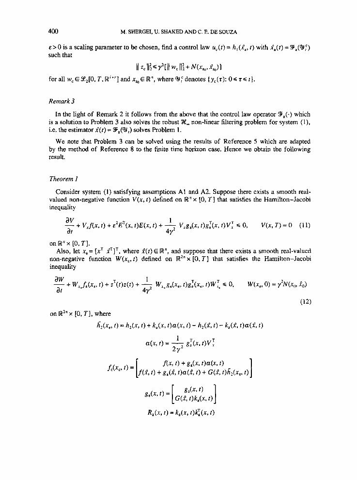
E > 0 is a scaling parameter to be chosen, find a control law u,(r) = h , ( i a , t ) with ia(t) = ?9;,(33 such that

II z c 11;s Y"Il wc 11;+ w,, f W ) l

for all w, EZ2[0, T , (wi+'l and x,E R", where 9: denotes ( y c ( 7 ) : 0s 7 s t ) .

Remark 3

In the light of Remark 2 it follows from the above that the control law operator 9',(-) which is a solution to Problem 3 also solves the robust %e, non-linear filtering problem for system (l), i.e. the estimator i ( t ) =

We note that Problem 3 can be solved using the results of Reference 5 which are adapted by the method of Reference 8 to the finite time horizon case. Hence we obtain the following result,

solves Problem 1.

Theorem 1

Consider system (1) satisfying assumptions A1 and A2. Suppose there exists a smooth real- valued non-negative function V(x, t ) defined on (w" x [0, TI that satisfies the Hamilton-Jacobi inequality

1 V(x, T ) = 0 (1 1)

av - + VJ(X, t ) + E ' E ~ ( x , t )E(x, t ) + 7 v,g,(x, r)gT(x, t>vT s 0, at 4Y

on Iw" x [0, T I . Also, let xe = [xT iTIT, where 2(t) E R", and suppose that there exists a smooth real-valued

non-negative function W(x, , t ) defined on R2" x [0, TI that satisfies the Hamilton-Jacobi inequality

aw 1 - + W.ymfe(xe, t ) + ZT(t)z(t) + - W.yege(xe, t)g%(xe, t )wl at 4Y2

09 W(xe, 0) = y 2 ~ ( x , , 2,)

(12) on R2" x [0, T I , where

h;(x,, t ) = h2(x, t ) + ka(x , t )a (x , t ) - A,(.?, t ) - k , ( i , t)a(2, t )

ROBUST X, NON-LINEAR ESTIMATION 40 1

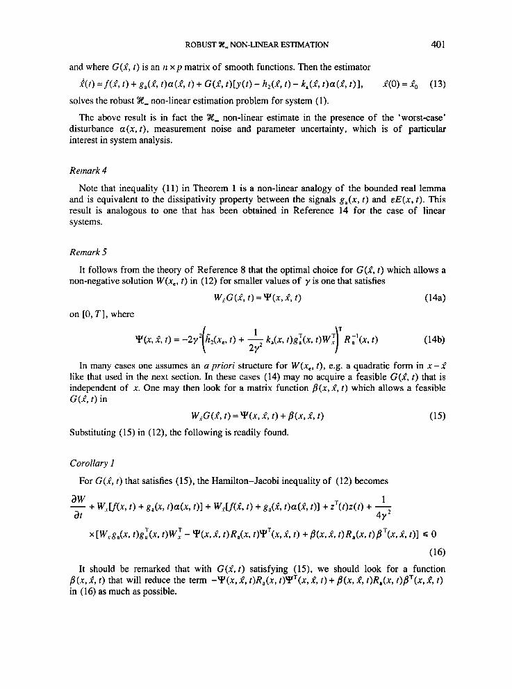
and where G(2, t ) is an n x p matrix of smooth functions. Then the estimator

k(t) =f(2, t ) + g , ( 2 , t)a(2, t ) + G(2, t ) [ y ( t ) - h , ( f , t ) - ka(2 , t)a(2, t ) ] , 2(0) = 2 0 (13) solves the robust X, non-linear estimation problem for system (1).

The above result is in fact the %e, non-linear estimate in the presence of the 'worst-case' disturbance a ( x , t ) , measurement noise and parameter uncertainty, which is of particular interest in system analysis.

Remark 4

Note that inequality (1 1) in Theorem 1 is a non-linear analogy of the bounded real lemma and is equivalent to the dissipativity property between the signals ga(x, t ) and EE(x , t) . This result is analogous to one that has been obtained in Reference 14 for the case of linear systems.

Remark 5

It follows from the theory of Reference 8 that the optimal choice for G(2, t ) which allows a non-negative solution W(x, , t ) in (12) for smaller values of y is one that satisfies

W,G(2, t ) = Y (x , 2, t )

on [0, T I , where

(14b) 1

ka(x, t)g;f(x, t )

In many cases one assumes an a priori structure for W(x, , t ) , e.g. a quadratic form in x - 2 like that used in the next section. In these cases (14) may no acquire a feasible G(2, t ) that is independent of x. One may then look for a matrix function B ( x , 2, t ) which allows a feasible G(2, t ) in

W,G(2, t ) = Y(x, 2, t ) + B(x , 2, t ) (15)

Substituting (15) in (12), the following is readily found.

Corollary 1

For G(2, t ) that satisfies (15), the Hamilton-Jacobi inequality of (12) becomes

x[W.Vga(x, t )g;f(x, t ) w l - ' y (x , 2, t)Ra(x, t)'yT(x, 2, t ) + b ( x , 2, t )Ra(x , t)BT(x, 2, t)l 0

(16) It should be remarked that with G(2,f ) satisfying (15), we should look for a function

B ( x , 2, t ) that will reduce the term -Y(x, 2, t )Ra(x , t)YT(x, 2, t ) + B ( x , 2, t )Ra(x , t )BT(x , 2, t ) in (16) as much as possible.

402 M. SHERGEI, U. SHAKED AND C. E. DE SOUZA

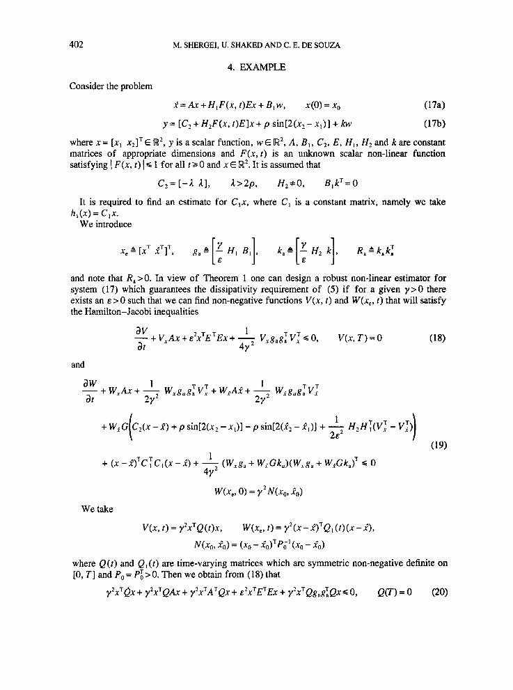
4. EXAMPLE

Consider the problem

i = A x + H , F ( x , t ) E x + B , w , x ( O ) = x , (17a)

(17b)

where x = [ x , x2ITE R2, y is a scalar function, w E R2, A , B , , C2, E , HI, Hz and k are constant matrices of appropriate dimensions and F ( x , t) is an unknown scalar non-linear function satisfying I F ( x , t) I d 1 for all t 2 0 and x f R2. It is assumed that

y = [C, + H 2 F ( x , t ) E ] x + p sin[2(x2 - x , ) ] + kw

C*=[-A A ] , L>2p, H,+O, B , k T = O

It is required to find an estimate for C,x, where C, is a constant matrix, namely we take

We introduce h,(x) = c ,x .

and note that R,>O. In view of Theorem 1 one can design a robust non-linear estimator for system (17) which guarantees the dissipativity requirement of (5) if for a given y>O there exists an E > 0 such that we can find non-negative functions V ( x , t) and W(x, , t) that will satisfy the Hamilton-Jacobi inequalities

V ( x , T ) = 0 av 2 T T 1 T T - + V,Ax + E x E EX + 7 V,vg,g, V , 0, at 4Y

and

W(xe, 0) = y 2 ~ ( x o , 20)

We take

V ( x , t ) = y2xTQ(t)x, W ( X , , t ) = y 2 ( X - 2 ) ' Q l ( t ) ( X - 2 ) ,

N ( x , , 2 0 ) = (x , - 2,)TPo' (xo - 2,)

where Q ( t ) and Q, (t) are time-varying matrices which are symmetric non-negative definite on [0, TI and P, = P i > 0. Then we obtain from (18) that

Y*X'QX + y2xTQAX + Y - X ' T A T QX + &'xTETEx + y2xTQg,gTQx s 0, Q(T) = 0 (20)

ROBUST X.., NON-LINEAR ESTIMATION 403

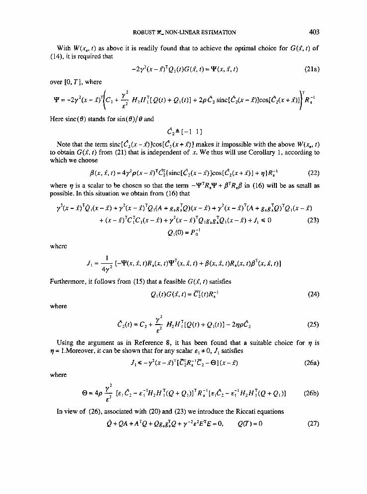
With W(x, , t ) as above it is readily found that to achieve the optimal choice for G ( f , t) of (14), it is required that

- 2 y 2 ( ~ - f ) T Q I ( t ) G ( f , r)=Y(x,f, t ) (21a)

over [0, TI, where

Y = -2y2(x - P)' Cz + 7 H2H:[ Q ( t ) + Q,(t)] + 2 p e z sinc[e,(x -P)]cos[e,(x +a)] R,' ( f r Here sinc (0) stands for sin( f3)/ 0 and

C2+1 11

Note that the term sinc[f,(x - f)]cos[c2(x + A?)] makes it impossible with the above W(x,, t) to obtain G ( f , t ) from (21) that is independent of x. We thus will use Corollary 1, according to which we choose

(22)

where 7 is a scalar to be chosen so that the term -YTRaY + BTRaB in (16) will be as small as possible. In this situation we obtain from (16) that

y z ( x - 2 ) T & I ( ~ - 2) + y 2 ( x - 2)'QI(A + g,g:Q)(x - 2 ) + y2(x - 2)T(A + gag:Q)'Q,(x - 2)

B ( x , 2, t ) = 4y2p(x - X^)~G( sinc[C2(x - ~^)lcos[C,(x + 211 + 7)~;'

+ (X - R)TC:C,(~ - 2) + y2(x - 2)TQlg,gfQl(x - 2) + 51 C 0 (23)

Q,O = PO'

where

Furthermore, it follows from (15) that a feasible G(2, I ) satisfies

Q , ( t ) G ( f , t ) = c ( t ) R ; ' where

(25) Y' E 2

c2(f) = C2 + - HzH:[Q(t) + Qi( t> l - ~ V P G Using the argument as in Reference 8, it has been found that a suitable choice for 7 is

q = l.Moreover, it can be shown that for any scalar E , +0, J, satisfies

J , s - y2 (X-XI)T[cRIIC2-O] (X- - ) (26a) where

(26b) Y 2 0 = 4p y- [ E ] e2 - &;'H,H:(Q + Q l ) l T R , ' [ ~ , e 2 - E;IH~HT(Q + Q , ) ] &

In view of (26), associated with (20) and (23) we introduce the Riccati equations

Q + QA + ATQ + Qg,giQ + Y - ~ E ' E ~ E = 0, Q(T) = 0 (27)

404 M. SHERGEI, U. SHAKED AND C. E. DE SOUZA

and

(28)

If for a given y>O we can find E > O and E , + O such that the above Riccati equations have bounded non-negative definite solutions on [0, T I , then the robust X, estimation problem for system (17) is solvable via the estimator of (13), which in this case is of the form

Qi + Q, (A + g,g;Q) + ( A + g,gTQ)TQi + Q,g,gTQl+ y-’C:Ci - GR-‘C, + 0 = 0 Q i (0) = PO‘

2= [A + aA(t)]2+ G(t)O, - [C, + AC(r)] 2- p sin[2(2*- .fi)1) where

G(t) = QF’( t )K’c ( f ) , AA(t) = g,gTQ(t), AC(t> = k,g:Q(t)

Note that since Q, (0) > 0, it follows from well-known results on Riccati equations that if there exists a bounded solution Q , ( t ) to (28) on [0, T I , then this solution is guaranteed to be symmetric positive definite on [0, TI .

To demonstrate the solution numerically, we choose A = 100, y = 1.7, p = 40,

A = [ 1, Il l=[ 0.1 0 0], k = [ O I], C1=[O 101 -25 -7.07

HI = [0 140IT, H, = 7000, E = [0 0.051

We treat the case of very large T ( T + m ) and find for E = 2942 and = 1500 that the Riccati equations (27) and (28) have bounded solutions on [0, T I . Moreover, these solutions converge numerically to

2.6363 O*OO14] Q, = [ 104.218 S*OOI] ’= [O-0014 0.1066 ’ 5.001 8.573

The resulting G, AA and AC are

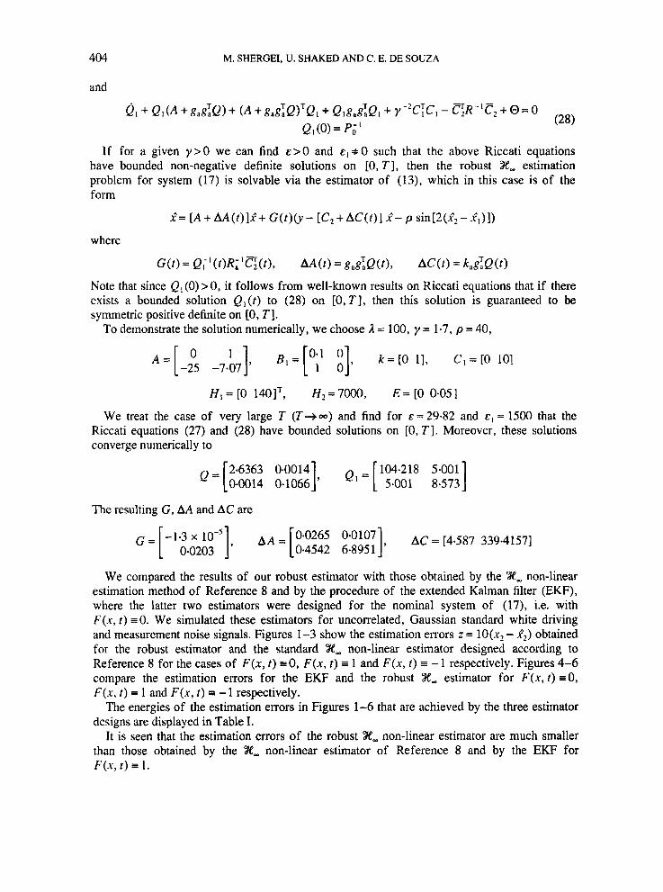
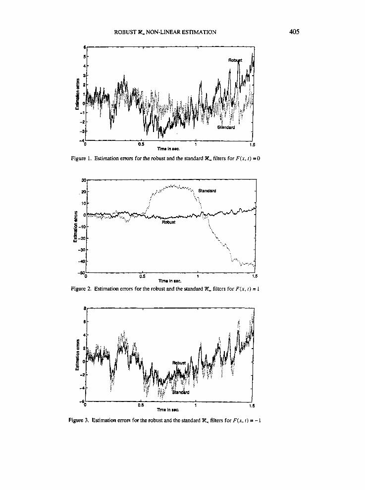
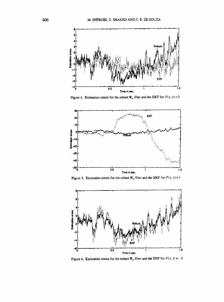
We compared the results of our robust estimator with those obtained by the X, non-linear estimation method of Reference 8 and by the procedure of the extended Kalman filter (EKF), where the latter two estimators were designed for the nominal system of (17), i.e. with F ( x , t ) = 0. We simulated these estimators for uncorrelated, Gaussian standard white driving and measurement noise signals. Figures 1-3 show the estimation errors z = 10(x2 - f2 ) obtained for the robust estimator and the standard X, non-linear estimator designed according to Reference 8 for the cases of F ( x , t ) = 0, F ( x , t ) = 1 and F ( x , t ) 3 - 1 respectively. Figures 4-6 compare the estimation errors for the EKF and the robust X, estimator for F ( x , t ) =O, F ( x , t ) 3 1 and F ( x , t ) s - 1 respectively.

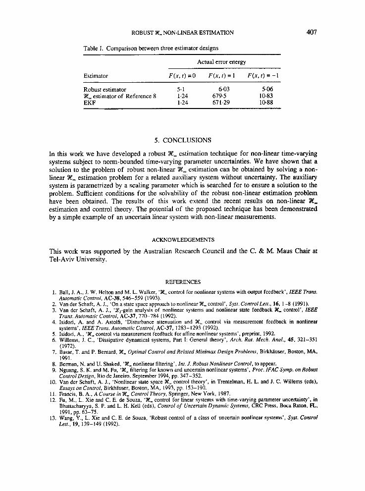
The energies of the estimation errors in Figures 1-6 that are achieved by the three estimator designs are displayed in Table I.

It is seen that the estimation errors of the robust X- non-linear estimator are much smaller than those obtained by the X, non-linear estimator of Reference 8 and by the EKF for F ( x , t ) = 1.

ROBUST X=. NON-LINEAR ESTIMATION

5 -10

3-20- - 2

-30

-40-

-r I

-

. .. .... . - \*

: f...,; - . ~ : .-.., 2 .‘

405

-4’ I 0 0.5 1 1 .5

Time in sec.

Figure 1. Estimation errors for the robust and the standard X- filters for F ( x , t ) = 0

0.5 1 1 .5 nme in soc.

Figure 3. Estimation errors for the robust and the standard X , filters for F ( x , t ) I - 1

406

E 1 -20

-30

-40-

M. SHERGEI, U. SHAKED AND C . E. DE SOUZA

. . -

x.. - :.:*!.,,: .

4

3 r %' 3 1

Lu 1 0 -1

-2

-3

-4 0 0.5 1 1.5 Tim in 8.c.

Figure 4. Estimation errors for the robust X , filter and the EKF for F ( x , 1 ) 0

301 I

Time in sec.

Figure 6. Estimation emrs for the robust X, filter and the EKF for F ( x , t ) = - I

ROBUST X, NON-LINEAR ESTIMATION 407

Table I. Comparison between three estimator designs

Actual error energy

Estimator F ( x , t ) = o F ( x , t ) = 1 F ( x , t ) = - 1

Robust estimator 5.1 6.03 5.06 X, estimator of Reference 8 1.24 679.5 10.83 EKF 1.24 67 1.29 10.88

5 . CONCLUSIONS

In this work we have developed a robust X, estimation technique for non-linear time-varying systems subject to norm-bounded time-varying parameter uncertainties. We have shown that a solution to the problem of robust non-linear X, estimation can be obtained by solving a non- linear X, estimation problem for a related auxiliary system without uncertainty. The auxiliary system is parametrized by a scaling parameter which is searched for to ensure a solution to the problem. Sufficient conditions for the solvability of the robust non-linear estimation problem have been obtained. The results of this work extend the recent results on non-linear X, estimation and control theory. The potential of the proposed technique has been demonstrated by a simple example of an uncertain linear system with non-linear measurements.

ACKNOWLEDGEMENTS

This work was supported by the Australian Research Council and the C. & M. Maus Chair at Tel-Aviv University.

REFERENCES

1. Ball, J. A., J. W. Helton and M. L. Walker, ‘ X , control for nonlinear systems with output feedback’, IEEE Trans.

2. Van der Schaft, A. J., ‘On a state space approach to nonlinear X , control’, Syst. Control Lett., 16, 1-8 (1991). 3. Van der Schaft, A. J., ‘S2-gain analysis of nonlinear systems and nonlinear state feedback X , control’, IEEE

4. Isidori, A. and A. Astolfi, ‘Disturbance attenuation and X, control via measurement feedback in nonlinear

5 . Isidori, A., ‘ X , control via measurement feedback for affine nonlinear systems’, preprint, 1992. 6. Willems, J. C., ‘Dissipative dynamical systems, Part I: General theory’, Arch. Rat. Mech. Anal., 45, 321-351

7 . Basar, T. and P. Bernard, X , Optimal Control and Related Minimax Design Problems, Birkhluser, Boston, MA,

8. Berman, N. and U. Shaked, ‘ X , nonlinear filtering’, Int. J . Robust Nonlinear Control, to appear. 9. Nguang, S. K. and M. Fu, ‘ X , filtering for known and uncertain nonlinear systems’, Proc. IFAC Symp. on Robust

Control Design, Rio de Janeiro, September 1994, pp. 347-352. 10. Van der Schaft, A. J., ‘Nonlinear state space X, control theory’, in Trentelman, H. L. and J. C. Willems (eds).

Essays on Control, Birkhauser, Boston, MA, 1993, pp. 153-190. 11. Francis, 9. A., A Course in X, ControlTheory, Springer, New York, 1987. 12. Fu, M., L. Xie and C. E. de Souza, ‘ X , control for linear systems with time-varying parameter uncertainty’, in

Bhattacharyya, S. P. and L. H. Kell (eds), Control of Uncertain Dynamic Systems, CRC Press, Boca Raton, FL,

13. Wang, Y., L. Xie and C. E. de Souza, ‘Robust control of a class of uncertain nonlinear systems’, Syst. Control

Automatic Control, AC-38,546-559 (1993).

Trans. Automatic Control, AC-37, 770-784 (1992).

systems’, IEEE Trans. Automatic Control, AC-37, 1283-1293 (1992).

(1972).

1991.

1991, pp. 63-75.

Letr., 19, 139-149 (1992).

408 M. SHERGEI, U. SHAKED AND C. E. DE SOUZA

14. Fu, M., C. E. de Souza and L. Xie, ‘X, estimation for uncertain systems’, Int. J . Robust Nonlinear Control, 2 ,

15. de Souza, C. E., M. Fu and U. Shaked, ‘A game theory approach to robust tracking’, Proc. Int. Workshop on

16. Doyle, J. C., K. Glover, P. P. Khargonekar and B. A. Francis, ‘State space solutions to standard X2 and X , control

87-105 (1992).

Robust Control, Santa Barbara, CA, 1993.

problems’, IEEE Trans. Automatic Control, AC-34,831-847 (1989).