robust and generalized nonparametric regression · standard methods such as kernel smoothing and...
TRANSCRIPT
Robust And Generalized Nonparametric Regression
T. Tony CaiDepartment of Statistics
The Wharton SchoolUniversity of Pennsylvania
http://stat.wharton.upenn.edu/˜tcai
Joint Work with Larry Brown and Harrison Zhou
1
Outline
• Introduction
• Robust Nonparametric Regression
– Median Coupling
• Nonparametric Regression in Exponential Families
– Mean-Matching VST for Exponential Families
• Discussion:
– Density Estimation
2

“A Gaussianization Machine”
‘Nonstandard’
Nonparametric
Regression
−→ Transformation −→Standard
Gaussian
Regression
3
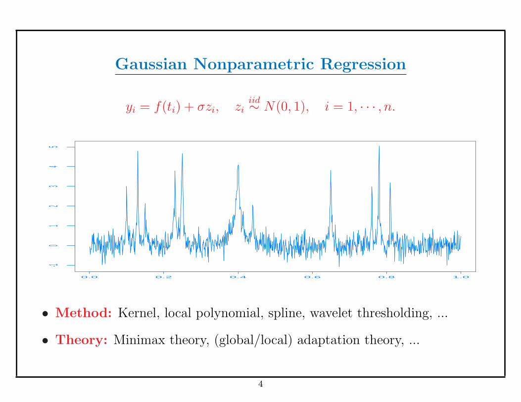
Gaussian Nonparametric Regression
yi = f(ti) + σzi, ziiid∼ N(0, 1), i = 1, · · · , n.
0.0 0.2 0.4 0.6 0.8 1.0
-10
12
34
5
• Method: Kernel, local polynomial, spline, wavelet thresholding, ...
• Theory: Minimax theory, (global/local) adaptation theory, ...
4
What About Non-Gaussian Noise?
“Nothing is Gaussian”
5
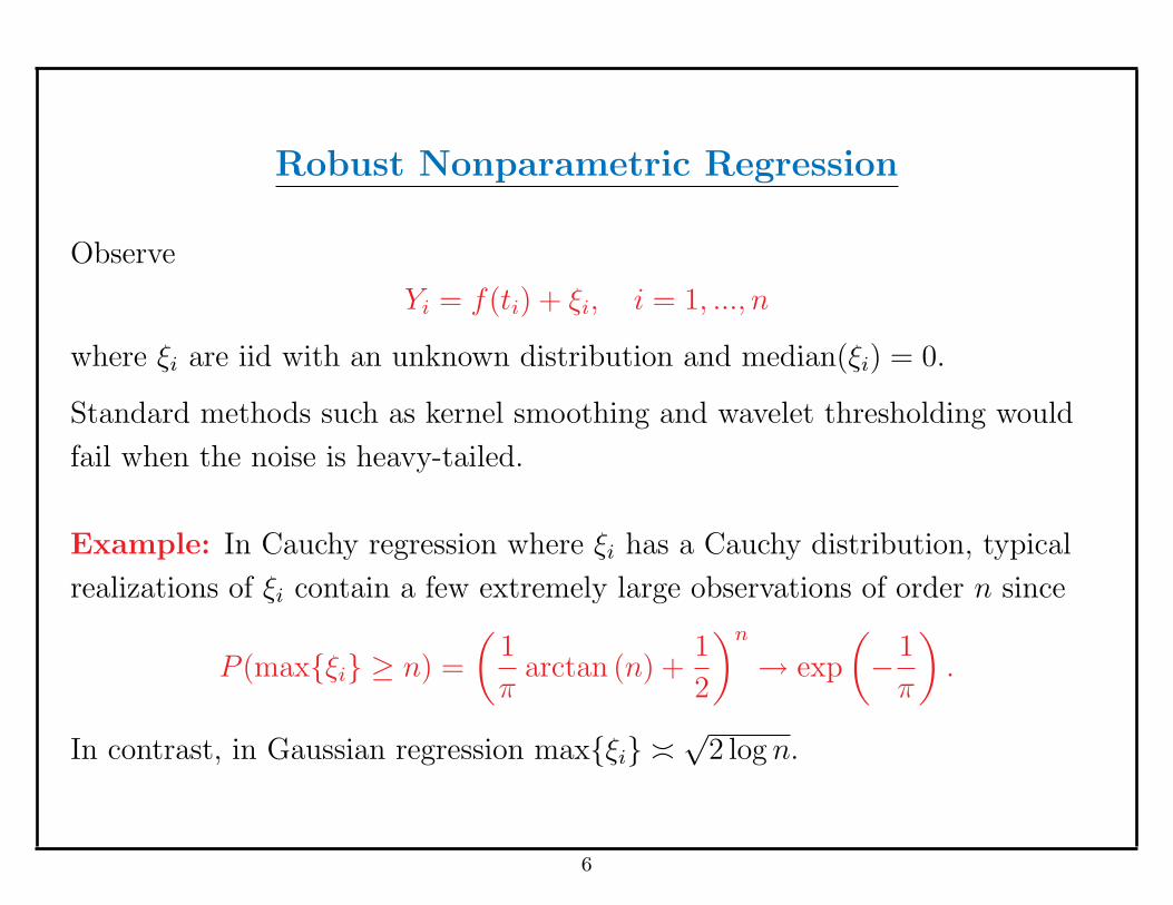
Robust Nonparametric Regression
Observe
Yi = f(ti) + ξi, i = 1, ..., n
where ξi are iid with an unknown distribution and median(ξi) = 0.
Standard methods such as kernel smoothing and wavelet thresholding would
fail when the noise is heavy-tailed.
Example: In Cauchy regression where ξi has a Cauchy distribution, typical
realizations of ξi contain a few extremely large observations of order n since
P (max{ξi} ≥ n) =
(1
πarctan (n) +
1
2
)n
→ exp
(− 1
π
).
In contrast, in Gaussian regression max{ξi} ³√
2 log n.
6
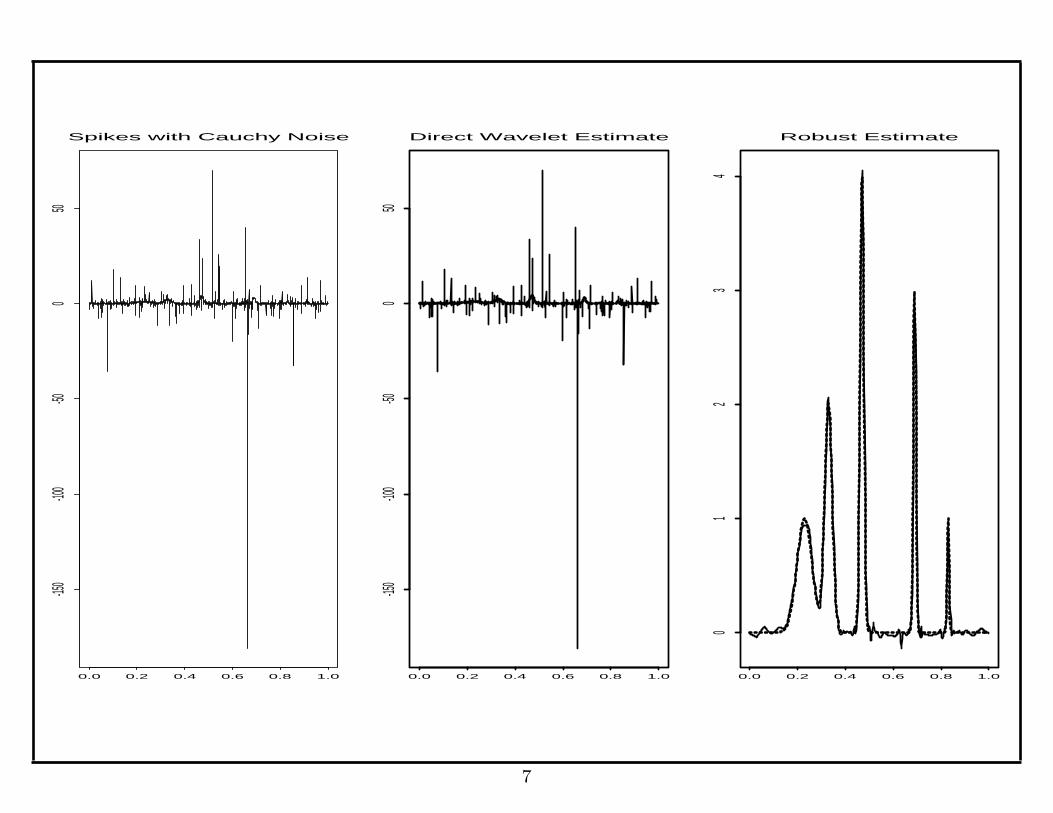
Spikes with Cauchy Noise
0.0 0.2 0.4 0.6 0.8 1.0
-150
-100
-500
50
0.0 0.2 0.4 0.6 0.8 1.0
-150
-100
-500
50
Direct Wavelet Estimate
0.0 0.2 0.4 0.6 0.8 1.0
01
23
4
Robust Estimate
7
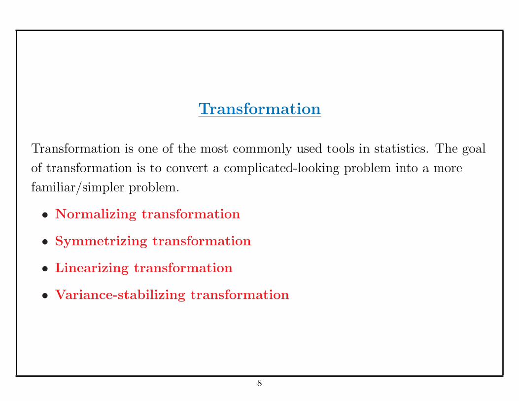
Transformation
Transformation is one of the most commonly used tools in statistics. The goal
of transformation is to convert a complicated-looking problem into a more
familiar/simpler problem.
• Normalizing transformation
• Symmetrizing transformation
• Linearizing transformation
• Variance-stabilizing transformation
8

Robust Regression
1. Binning & Taking Median: Divide the indices {1, ..., n} into T
equilength bins {Ij : j = 1, ..., T} of size m and let
Y ∗j = median(Yi : i ∈ Ij).
Then Y ∗j can be treated as if it were a normal random variable with mean
g( jT) = f( j
T) + bm and variance σ2 = 1/(4mh2(0)), where h is the density
function of εi and
bm = E{median(ξ1, . . . , ξm)}. (1)
Both the variance σ2 and the bias bm can be estimated easily.
2. Gaussian Regression: Applying your favorite Gaussian regression
procedure to {Y ∗j , j = 1, ..., T} to yield an estimator g. The regression
function f is then estimated by f = g− bm where bm is an estimator of the
bias bm.
9
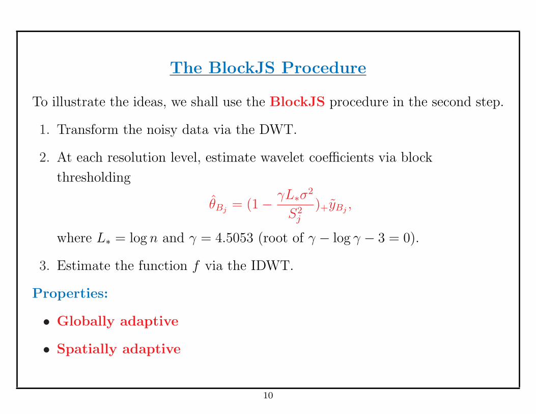
The BlockJS Procedure
To illustrate the ideas, we shall use the BlockJS procedure in the second step.
1. Transform the noisy data via the DWT.
2. At each resolution level, estimate wavelet coefficients via block
thresholding
θBj= (1− γL∗σ2
S2j
)+yBj,
where L∗ = log n and γ = 4.5053 (root of γ − log γ − 3 = 0).
3. Estimate the function f via the IDWT.
Properties:
• Globally adaptive
• Spatially adaptive
10
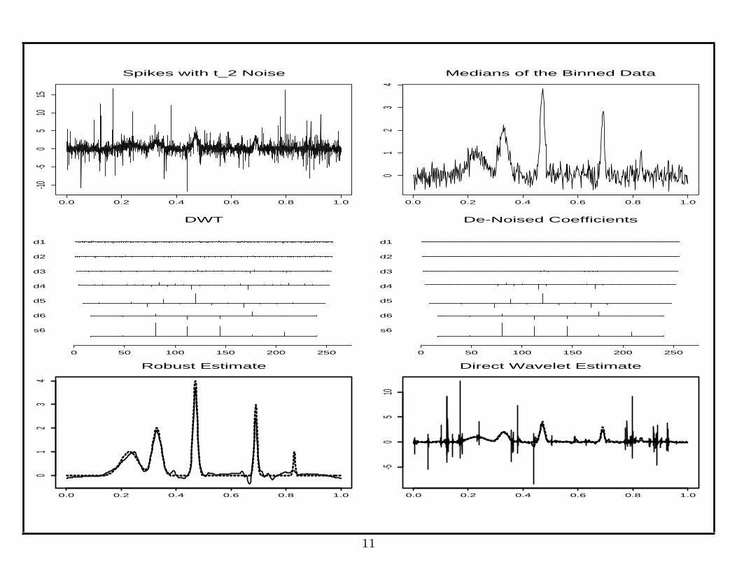
Spikes with t_2 Noise
0.0 0.2 0.4 0.6 0.8 1.0
-10-5
05
1015
Medians of the Binned Data
0.0 0.2 0.4 0.6 0.8 1.0
01
23
4
0 50 100 150 200 250
s6
d6
d5
d4
d3
d2
d1
DWT
0 50 100 150 200 250
s6
d6
d5
d4
d3
d2
d1
De-Noised Coefficients
0.0 0.2 0.4 0.6 0.8 1.0
01
23
4
Robust Estimate
0.0 0.2 0.4 0.6 0.8 1.0
-50
510
Direct Wavelet Estimate
11
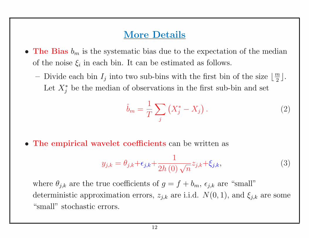
More Details
• The Bias bm is the systematic bias due to the expectation of the median
of the noise ξi in each bin. It can be estimated as follows.
– Divide each bin Ij into two sub-bins with the first bin of the size bm2c.
Let X∗j be the median of observations in the first sub-bin and set
bm =1
T
∑j
(X∗
j −Xj
). (2)
• The empirical wavelet coefficients can be written as
yj,k = θj,k+εj,k+1
2h (0)√
nzj,k+ξj,k, (3)
where θj,k are the true coefficients of g = f + bm, εj,k are “small”
deterministic approximation errors, zj,k are i.i.d. N(0, 1), and ξj,k are some
“small” stochastic errors.
12
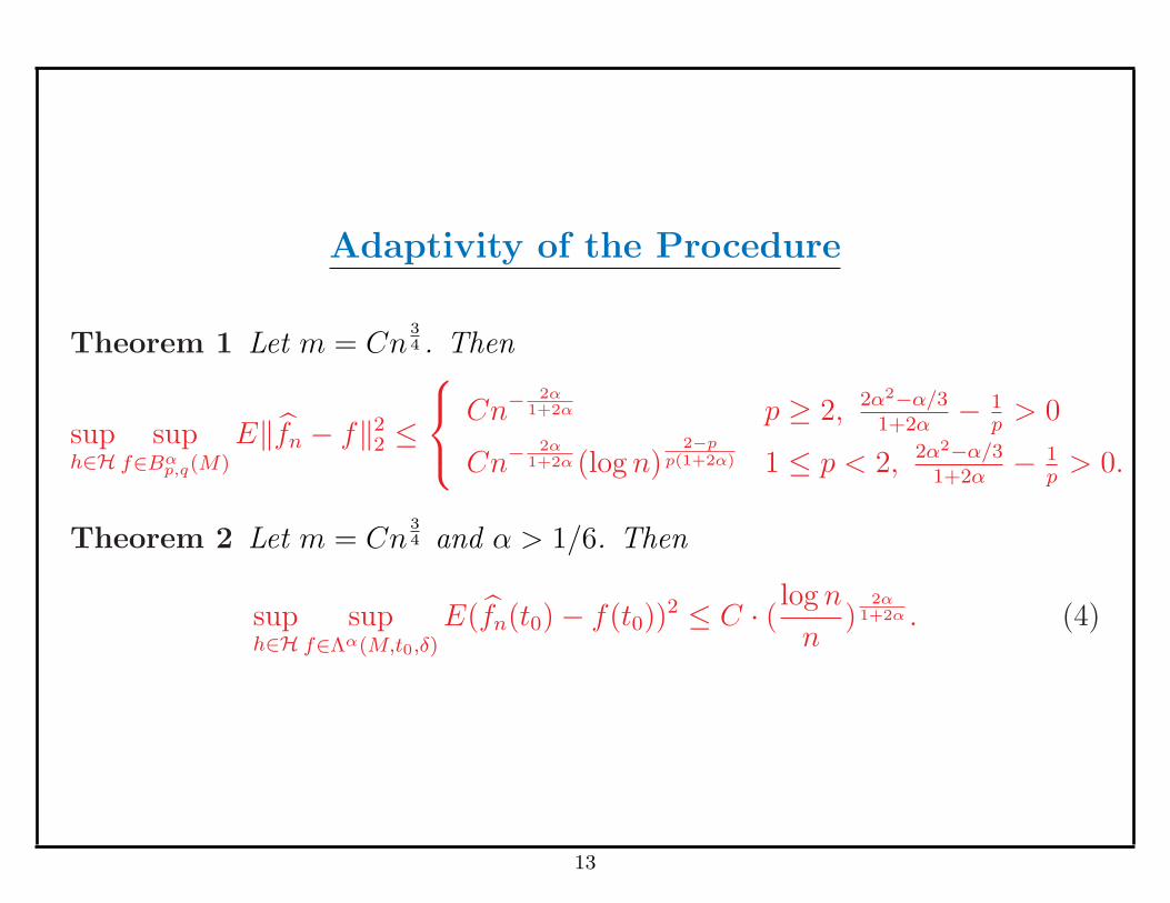
Adaptivity of the Procedure
Theorem 1 Let m = Cn34 . Then
suph∈H
supf∈Bα
p,q(M)
E‖fn − f‖22 ≤
Cn−2α
1+2α p ≥ 2, 2α2−α/31+2α
− 1p
> 0
Cn−2α
1+2α (log n)2−p
p(1+2α) 1 ≤ p < 2, 2α2−α/31+2α
− 1p
> 0.
Theorem 2 Let m = Cn34 and α > 1/6. Then
suph∈H
supf∈Λα(M,t0,δ)
E(fn(t0)− f(t0))2 ≤ C · ( log n
n)
2α1+2α . (4)
13
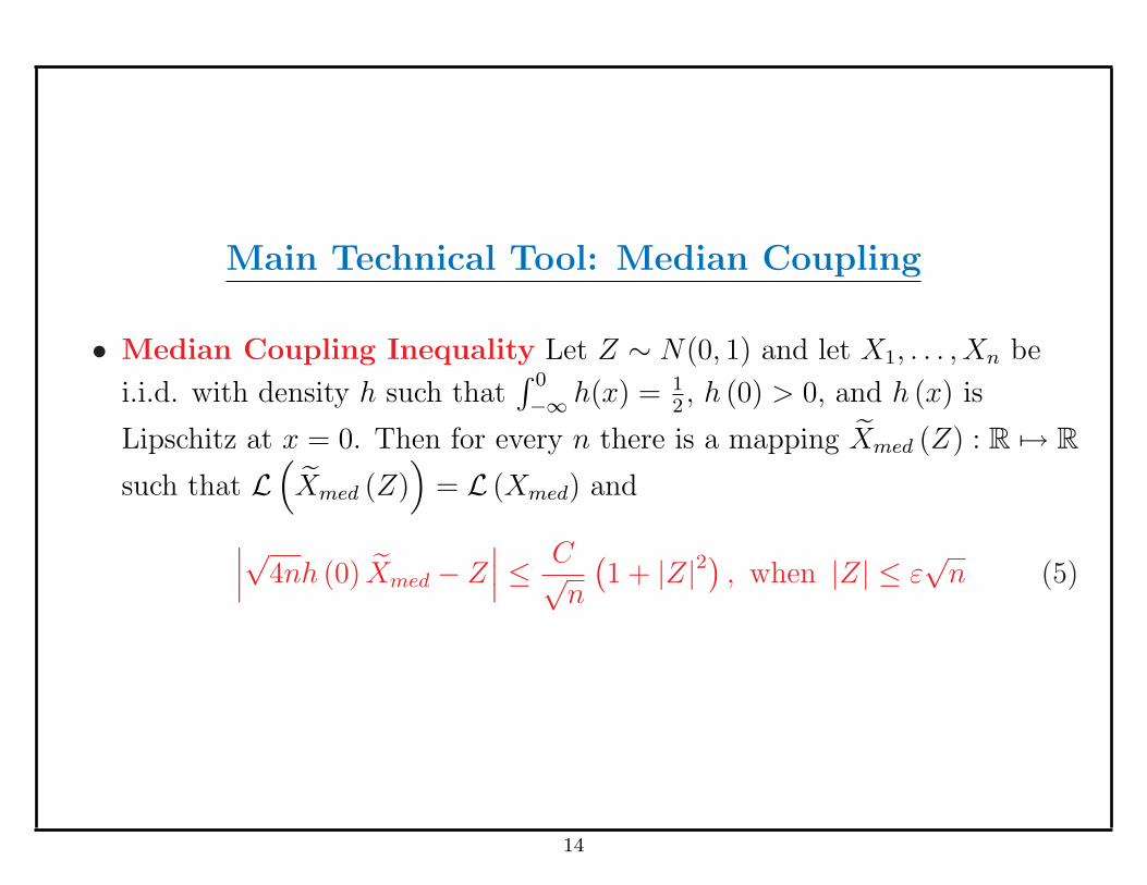
Main Technical Tool: Median Coupling
• Median Coupling Inequality Let Z ∼ N(0, 1) and let X1, . . . , Xn be
i.i.d. with density h such that∫ 0
−∞ h(x) = 12, h (0) > 0, and h (x) is
Lipschitz at x = 0. Then for every n there is a mapping Xmed (Z) : R 7→ Rsuch that L
(Xmed (Z)
)= L (Xmed) and
∣∣∣√
4nh (0) Xmed − Z∣∣∣ ≤ C√
n
(1 + |Z|2) , when |Z| ≤ ε
√n (5)
14
Remark
If the error distribution is known/assumed to be symmetric, much stronger
results can be obtained. (In this case, bm ≡ 0.)
• Asymptotic Equivalence: The medians {Y ∗j } can be shown to be
asymptotically equivalent to a Gaussian experiment.
• Smaller Bin Size: For robust estimation of the regression function, the
bin size can be taken to be logarithmic.
• Estimating Functionals: Similar results can be derived for estimating
functionals such as linear or quadratic functionals.
15
Generalized Nonparametric Regression
16

Other Nonparametric Function Estimation Models
• White Noise Model:
dY (t) = f(t)dt + εdW (t)
where W is a standard Brownian motion.
• Density Estimation: X1, X2, · · · , Xni.i.d.∼ f.
• Poisson Regression: Xi ∼ Poisson(λ(ti)), i = 1, ..., n.
• Binomial Regression: Xi ∼ Binomial(r, p(ti)), i = 1, ..., n.
• ...
17
Asymptotic Equivalence Theory
• Regression ⇐⇒ White Noise
Brown & Low (1996), Brown, Cai, Low, & Zhang (2002).
• Density Estimation ⇐⇒ White Noise
Nussbaum (1996), Brown, Carter, Low, & Zhang (2004).
• Density Estimation ⇐⇒ Poisson Regression (Poissonization)
Low and Zhou (2007).
18

Natural Exponential Families
Let X1, X2, ..., Xn be a random sample from the distribution in the natural
exponential family (NEF) with the pdf/pmf
f(x|ξ) = eξx−ψ(ξ)h(x).
The mean and variance are µ(ξ) = ψ′(ξ), and σ2(ξ) = ψ′′(ξ) respectively.
In the subclass with a quadratic variance function (QVF),
σ2 ≡ V (µ) = v0 + v1µ + v2µ2. (6)
We shall write
X1, X2, ..., Xn ∼ NQ(µ).
NEF-QVF families consist of six important distributions, three continuous:
Normal, Gamma, and NEF-GHS distributions; three discrete: Binomial,
Negative Binomial, and Poisson (see, e.g., Morris (1982) and Brown
(1986)).
19
Variance Stabilizing Transformation (VST)
Set X =∑n
i=1 Xi. Then
√n(X/n− µ(ξ))
L−→ N(0, V (µ(ξ))).
The VST is a function G : IR → IR such that
G′(µ) = V − 12 (µ). (7)
The delta method yields
√n{G(X/n)−G(µ(ξ))} L−→ N(0, 1).
The variance stabilizing properties can be improved by using
H(X) = G(X + a
n + b)
with suitable choice of a and b. See, e.g., Anscombe (1948).
20
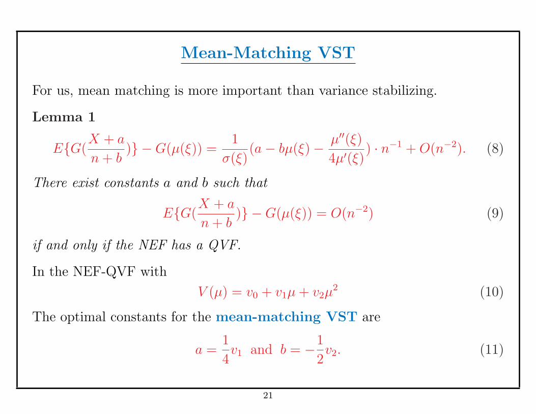
Mean-Matching VST
For us, mean matching is more important than variance stabilizing.
Lemma 1
E{G(X + a
n + b)} −G(µ(ξ)) =
1
σ(ξ)(a− bµ(ξ)− µ′′(ξ)
4µ′(ξ)) · n−1 + O(n−2). (8)
There exist constants a and b such that
E{G(X + a
n + b)} −G(µ(ξ)) = O(n−2) (9)
if and only if the NEF has a QVF.
In the NEF-QVF with
V (µ) = v0 + v1µ + v2µ2 (10)
The optimal constants for the mean-matching VST are
a =1
4v1 and b = −1
2v2. (11)
21
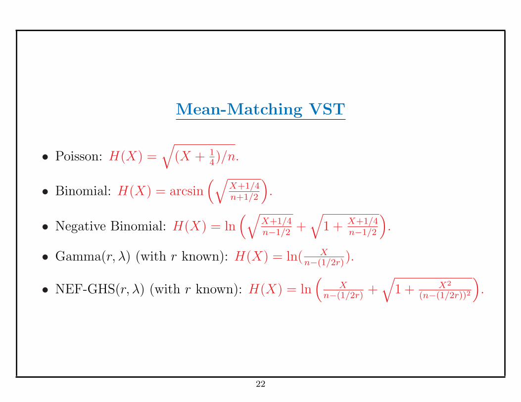
Mean-Matching VST
• Poisson: H(X) =√
(X + 14)/n.
• Binomial: H(X) = arcsin(√
X+1/4n+1/2
).
• Negative Binomial: H(X) = ln(√
X+1/4n−1/2
+√
1 + X+1/4n−1/2
).
• Gamma(r, λ) (with r known): H(X) = ln( Xn−(1/2r)
).
• NEF-GHS(r, λ) (with r known): H(X) = ln(
Xn−(1/2r)
+√
1 + X2
(n−(1/2r))2
).
22

Bias
Poisson(lambda)
0 1 2 3 4
-0.2-0.1
0.00.1
0.20.3
+
+
+
+
++++++++++++++++++++++++++++++++++++++++++++++++++++++++++++++++++++++++++++++++++++++++++++++++
c=0+ c=1/4
c=3/8
Variance
Poisson(lambda)
0 2 4 6 8 10
0.10.2
0.30.4
+
+
+
+
+
+
+
+
+
+++++++++++++
++++++++++++++++++++++++++++++++++++++++++++++++++++++++++++++++++++++++++++++
c=0+ c=1/4
c=3/8
22-1
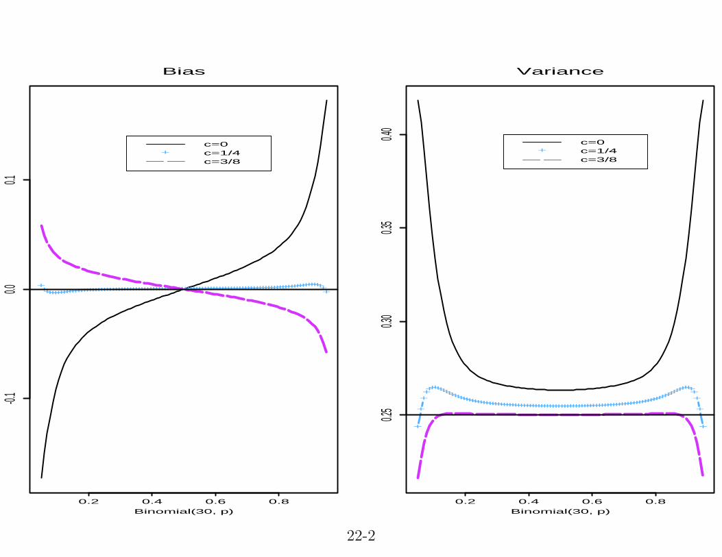
Bias
Binomial(30, p)
0.2 0.4 0.6 0.8
-0.10.0
0.1
+++++++++++++++++++++++++++++++++
++++++++++++++++++++++++++++++++++++++++++++++++++++++++++++++++++
+
c=0+ c=1/4
c=3/8
Variance
Binomial(30, p)
0.2 0.4 0.6 0.8
0.25
0.30
0.35
0.40
+
+
+++++++++++++++++++++++++++++++++++++++++++++++++++++++++++++++++++++++++++
+++++++++++
+++++++++
+
+
+
c=0+ c=1/4
c=3/8
22-2
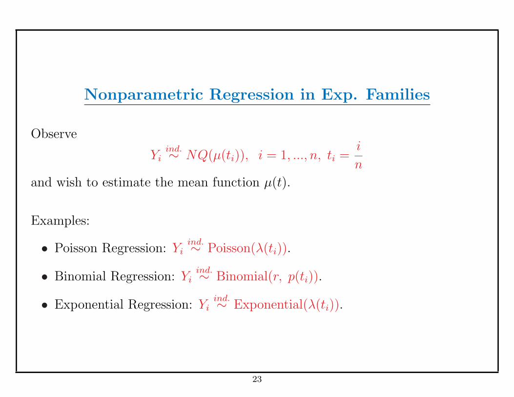
Nonparametric Regression in Exp. Families
Observe
Yiind.∼ NQ(µ(ti)), i = 1, ..., n, ti =
i
n
and wish to estimate the mean function µ(t).
Examples:
• Poisson Regression: Yiind.∼ Poisson(λ(ti)).
• Binomial Regression: Yiind.∼ Binomial(r, p(ti)).
• Exponential Regression: Yiind.∼ Exponential(λ(ti)).
23
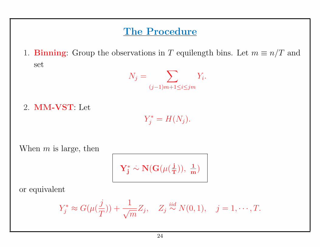
The Procedure
1. Binning: Group the observations in T equilength bins. Let m ≡ n/T and
set
Nj =∑
(j−1)m+1≤i≤jm
Yi.
2. MM-VST: Let
Y ∗j = H(Nj).
When m is large, then
Y∗j
.∼ N(G(µ( jT
)), 1m
)
or equivalent
Y ∗j ≈ G(µ(
j
T)) +
1√m
Zj, Zjiid∼ N(0, 1), j = 1, · · · , T.
24
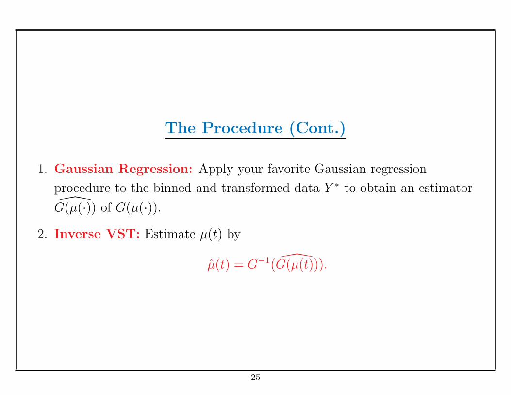
The Procedure (Cont.)
1. Gaussian Regression: Apply your favorite Gaussian regression
procedure to the binned and transformed data Y ∗ to obtain an estimator
G(µ(·)) of G(µ(·)).2. Inverse VST: Estimate µ(t) by
µ(t) = G−1(G(µ(t))).
25
Nonparametric Regression in Exp. Families
1. Binning & Mean Matching VST
2. BlockJS
3. Inverse VST
26

Example: Poisson Regression
t
0.0 0.2 0.4 0.6 0.8 1.0
100150
200
Noisy Signal
0 100 200 300 400 500
s6
d6
d5
d4
d3
d2
d1
DWT
t
0.0 0.2 0.4 0.6 0.8 1.0
1011
1213
1415
Estimate of Square Root
t
0.0 0.2 0.4 0.6 0.8 1.0
1012
14
Root Transformed Signal
0 100 200 300 400 500
s6
d6
d5
d4
d3
d2
d1
De-Noised Coefficients
t
0.0 0.2 0.4 0.6 0.8 1.0
100120
140160
180200
220
Final Estimate
27
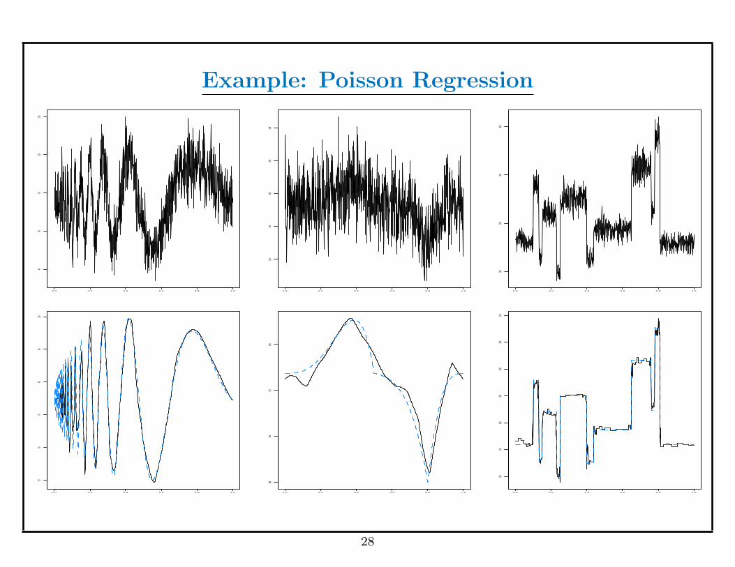
Example: Poisson Regression
0.0 0.2 0.4 0.6 0.8 1.0
4060
80100
120
0.0 0.2 0.4 0.6 0.8 1.0
140160
180200
220
0.0 0.2 0.4 0.6 0.8 1.0
100200
300400
0.0 0.2 0.4 0.6 0.8 1.0
5060
7080
90100
0.0 0.2 0.4 0.6 0.8 1.0
150160
170180
0.0 0.2 0.4 0.6 0.8 1.0
100150
200250
300350
400
28
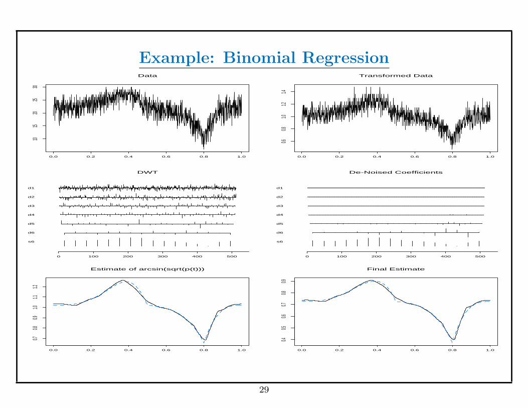
Example: Binomial Regression
0.0 0.2 0.4 0.6 0.8 1.0
1015
2025
30
Data
0.0 0.2 0.4 0.6 0.8 1.0
0.60.8
1.01.2
1.4
Transformed Data
0 100 200 300 400 500
s6
d6
d5
d4
d3
d2
d1
DWT
0 100 200 300 400 500
s6
d6
d5
d4
d3
d2
d1
De-Noised Coefficients
0.0 0.2 0.4 0.6 0.8 1.0
0.70.8
0.91.0
1.11.2
Estimate of arcsin(sqrt(p(t)))
0.0 0.2 0.4 0.6 0.8 1.0
0.40.5
0.60.7
0.80.9
Final Estimate
29
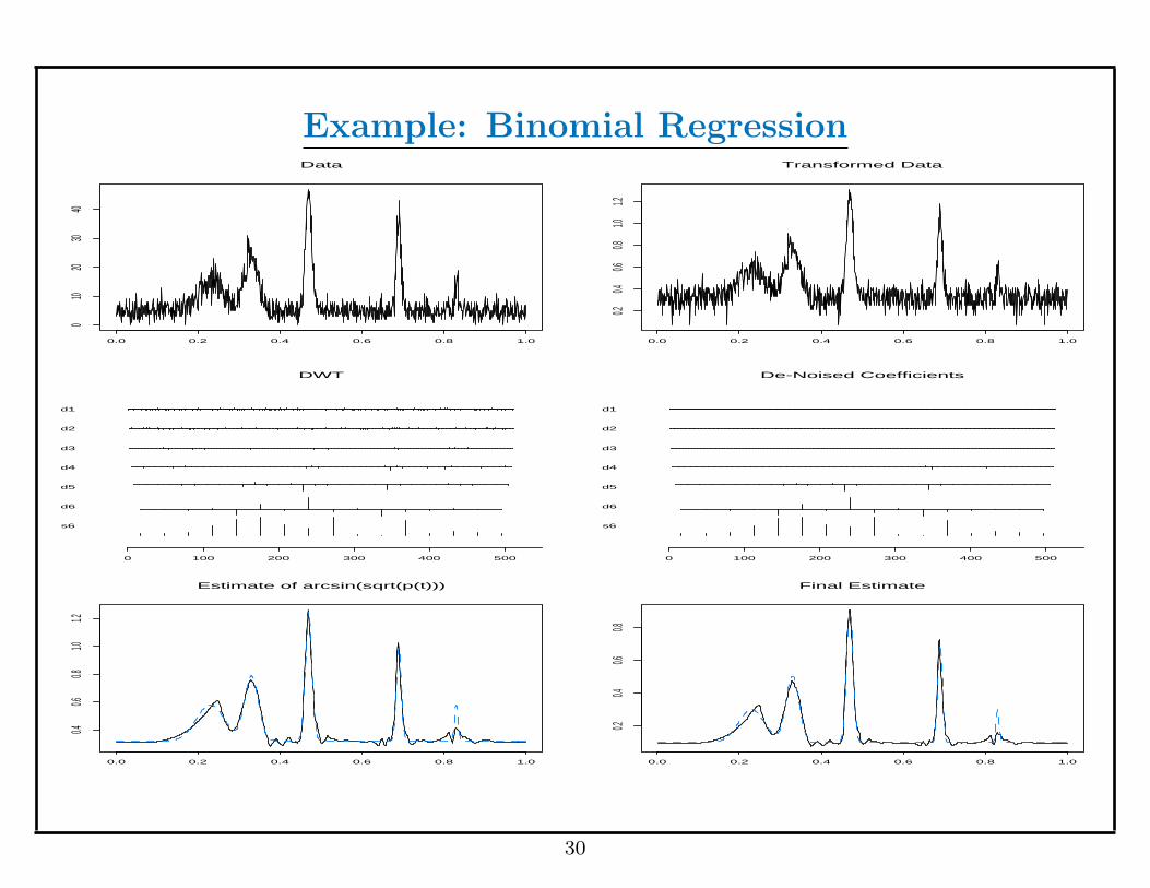
Example: Binomial Regression
0.0 0.2 0.4 0.6 0.8 1.0
010
2030
40
Data
0.0 0.2 0.4 0.6 0.8 1.0
0.20.4
0.60.8
1.01.2
Transformed Data
0 100 200 300 400 500
s6
d6
d5
d4
d3
d2
d1
DWT
0 100 200 300 400 500
s6
d6
d5
d4
d3
d2
d1
De-Noised Coefficients
0.0 0.2 0.4 0.6 0.8 1.0
0.40.6
0.81.0
1.2
Estimate of arcsin(sqrt(p(t)))
0.0 0.2 0.4 0.6 0.8 1.0
0.20.4
0.60.8
Final Estimate
30
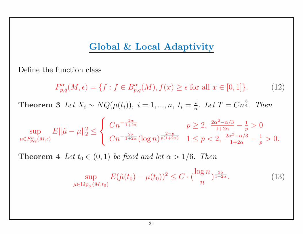
Global & Local Adaptivity
Define the function class
Fαp,q(M, ε) = {f : f ∈ Bα
p,q(M), f(x) ≥ ε for all x ∈ [0, 1]}. (12)
Theorem 3 Let Xi ∼ NQ(µ(ti)), i = 1, ..., n, ti = in. Let T = Cn
34 . Then
supµ∈F α
p,q(M,ε)
E‖µ− µ‖22 ≤
Cn−2α
1+2α p ≥ 2, 2α2−α/31+2α
− 1p
> 0
Cn−2α
1+2α (log n)2−p
p(1+2α) 1 ≤ p < 2, 2α2−α/31+2α
− 1p
> 0.
Theorem 4 Let t0 ∈ (0, 1) be fixed and let α > 1/6. Then
supµ∈Lipα(M ;t0)
E(µ(t0)− µ(t0))2 ≤ C · ( log n
n)
2α1+2α . (13)
31
Density Estimation
• Density estimation can be treated in a similar way. X1, ...,Xniid∼ f .
1. Binning: Bin the observations into m groups, Nj = #{Xi : Xi ∈ Gj}.2. Root Transform: Yj =
√Nj+1/4
m.
3. BlockJS
4. Unroot Transform
32
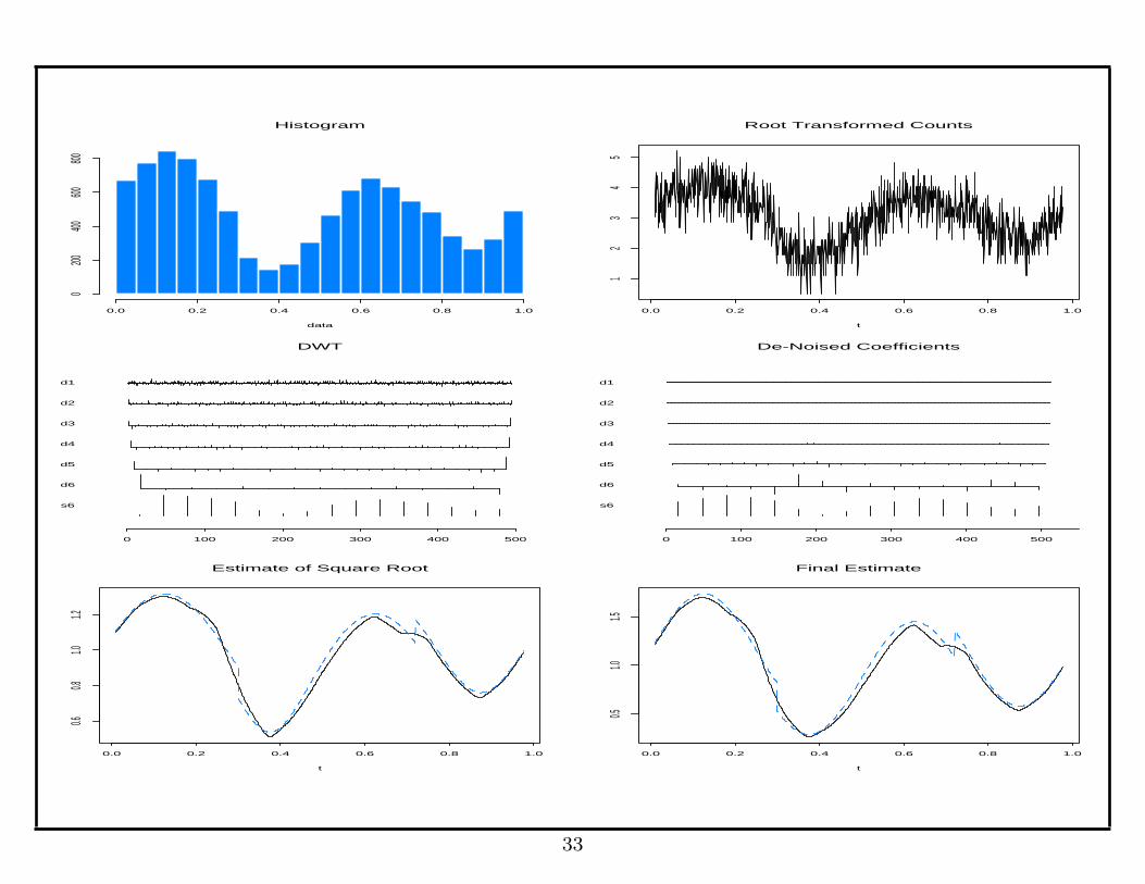
0.0 0.2 0.4 0.6 0.8 1.0
0200
400600
800
data
Histogram
t
0.0 0.2 0.4 0.6 0.8 1.0
12
34
5
Root Transformed Counts
0 100 200 300 400 500
s6
d6
d5
d4
d3
d2
d1
DWT
0 100 200 300 400 500
s6
d6
d5
d4
d3
d2
d1
De-Noised Coefficients
t
0.0 0.2 0.4 0.6 0.8 1.0
0.60.8
1.01.2
Estimate of Square Root
t
0.0 0.2 0.4 0.6 0.8 1.0
0.51.0
1.5
Final Estimate
33
Summary
‘Nonstandard’
Nonparametric
Regression
−→ Transformation −→Standard
Gaussian
Regression
34
Papers
Brown, L. D., Cai, T. & Zhou, H. (2008). Robust nonparametric
estimation via wavelet median regression. Ann. Statist. 36, 2055-2084.
Cai, T. & Zhou, H. (2009). Asymptotic equivalence and adaptive
estimation for robust nonparametric regression. Ann. Statist. 37, in
press.
Brown, L. D., Cai, T. & Zhou, H. (2009). Nonparametric regression in
exponential families. Technical Report.
Available at: http://stat.wharton.upenn.edu/∼tcai
35