Robust Adaptive Terrain-Relative NavigationShandor Dektor

Department of Aeronautics and AstronauticsStanford UniversityStanford, CA 94305

Email: sgd@stanford.edu

Stephen RockDepartment of Aeronautics and Astronautics

Stanford UniversityStanford, CA 94305

Email: rock@stanford.edu

Abstract—Terrain-Relative Navigation (TRN) is a technique forlocalizing a vehicle in GPS-denied environments. TRN augmentsa dead-reckoned solution with continuous position fixes based oncorrelations with a pre-stored map. In underwater applicationsTRN accuracy on the order of 3m has been demonstrated,however convergence to incorrect solutions has been observedwhen operating for extended periods over featureless terrain.Specifically, the TRN filter can become overconfident in anincorrect position fix.

Previous work by the authors introduced an adaptive tech-nique for mitigating over-confidence in uninformative terrain.Specifically, the algorithm exponentially down-weights the prob-abilities with a factor α between zero and one, based on the esti-mated terrain information. This paper focuses on understandingthe source of false fixes in uninformative terrain, and uses thisinsight to develop the method behind the adaptive technique.

This paper shows that the cause of false fixes using standardTRN weighting in information-poor regions is the assumptionthat the terrain is uncorrelated. It also introduces a method toanalyze the probability of false peaks using the standard TRNmeasurement weighting. This analysis is an extension of workin the statistics community on robust adjusted likelihood ratios,and is used to bound the probability of large false peaks.

The resulting robust, adaptive technique is capable of real-time operation and its effectiveness is demonstrated in simulationand with field data from MBARI AUV runs over flat terrain inMonterey Bay.

I. INTRODUCTION

Terrain-Relative Navigation (TRN) is an emerging tech-nique for localizing a vehicle in the underwater environment.TRN offers a means to eliminate drift accrued during deadreckoning by matching range measurements of the terrain toan on-board terrain map. The TRN concept was first deployedas the cruise missile guidance system TERCOM (TerrainContour Matching), which used a batch correlation of altimetermeasurements against an a priori map to generate a positionestimate [1].

TRN was adapted to autonomous underwater vehicles(AUVs) starting in the 1990s [2] [3] and TRN packages arenow available on commercial vehicles such as the HUGINAUV [4]. Map-relative position estimates are particularlyvaluable for AUVs as they reduce the necessity of surfac-ing for GPS fixes or deploying USBL or LBL positioningsystems. Further, many return-to-site underwater missions areto locations identified in a map, and since underwater mapscan be inaccurately geo-referenced, a map-relative position isnecessary [5].

In informative terrain TRN accuracy is typically on the orderof the map resolution. Accuracy of a few meters has beendemonstrated in field trials using MBARIs Dorado-class AUVsin Monterey Bay [6], and similar performance was observedin field trials using the HUGIN AUV in Ostfjords [7].

When operating over featureless terrain for an extendedperiod, converging to an overconfident, incorrect solution -a false fix - is a recognized issue with TRN filters [8] [9].False fixes greatly reduce the value of a TRN estimate. Anincorrect TRN estimate can result in failure to accomplish amission, and in the case of close proximity operations, canlead to trajectories intersecting the terrain.

This has motivated a large amount of effort towards un-derstanding and reducing the incidence of false fixes due touninformatve terrain. Simulations in [10] showed that falsefixes increase with the amount of noise in the map. Theinformation metrics developed in [11] were used to selectinformative regions of terrain for correlation. The integritymethods in [7] reject TRN position fixes if the variation inthe terrain contour is insufficient.

The adaptive method presented in [12] is designed to slowconvergence in uninformative terrain to prevent false fixes.This paper focuses on understanding the source of false fixesin uninformative terrain, and uses this to develop the methodbehind the adaptive technique.

In the standard formulation of the TRN problem, a Gaussianlikelihood function is typically used to perform the measure-ment update. That is:

L(x)standard = p(z, h|x)standard = η exp

(−(z − z)2

2(σ2map + σ2

sensor)

)(1)

where z is the measurement, z = h(x) is the estimatedmeasurement from the map, and σ2

map and σ2sensor are the map

and sensor noise.This paper shows that this formulation implicitly assumes

that the vehicle is operating over informative terrain, and thatthis results in false fixes when operating over uninformativeterrain. This assumption enters the measurement update asa probabilistic terrain model that characterizes the degree ofspatial correlation in the terrain; in standard TRN, the terrainis assumed to be uncorrelated. This assumption is reasonablewhen the terrain correlation is small with respect to error inthe map, but results in false peaks when the terrain correlation

is large with respect to map error.The relation between the level of terrain correlation and

the occurrence of false peaks using standard TRN correlationis demonstrated using simulated informative and uninforma-tive terrains generated from probabilistic terrain models. Theprobabilistic terrain models employed are Gaussian and arecommonly used in the Geographic Information System (GIS)community to characterize spatial correlation. Likelihood sur-faces are computed using the standard uncorrelated terrainmodel and the known Gaussian terrain model for both cases.Both probabilistic terrain models have comparable perfor-mance in informative terrain, but in uninformative terrain thecorrelated Gaussian terrain model eliminates the false peaksthat arise using standard TRN correlation. This motivated thedevelopment of the adaptive technique presented in [12].

The result of this development is that the likelihood functionused in the measurement update becomes

L(x)adjusted = L(x)αstandard = p(z, h|x)αstandard (2)

Specifically, this adaptive adaptive method exponentiallydown-weights the probabilities calculated using the standardTRN algorithm to account for the false peaks introducedby the uncorrelated terrain model. This method is based onanalyzing the likelihood of false peaks using the standardTRN measurement weighting, and is an extension of work inthe statistics community on robust adjusted likelihood ratios[13]. This analysis shows that adjusting the probabilities witha factor α between zero and one, based on the estimatedterrain information, can eliminate the large false peaks usingthe standard TRN weighting. Here, terrain information isthe amount of variance in the expected measurements thatcan not be attributed to map error. This method achievesgood performance in simulated runs on both informative anduninformative terrain, at a computational cost comparable tousing the standard TRN weighting.

This paper is organized as follows. Section II outlines thebasics of the TRN problem. Section III describes how terrainmodels enter in to the measurement update, and how the stan-dard TRN assumption results in overconfidence. Section IVintroduces the method of mitigating false-fixes by matchingfalse peak likelihoods. Section V compares results using thestandard and adaptive TRN algorithms in offline runs usingfield data gathered in flat terrain in Monterey Bay.

II. THE BASIC TRN PROBLEM

The goal of a TRN estimator is to localize a vehicle withrespect to the underlying terrain. This is accomplished usingan estimation filter that fuses a vehicle motion model with anobservation model.

The filter presented here is characteristic of TRN applica-tions. It consists of three components: a particle filter usedto model the uncertainty in the vehicle position, a kinematicprocess model to propagate the vehicle dead reckoning esti-mate and associated error, and a range measurement model toestimate the vehicle position given range measurements and aterrain.

A. TRN Filter

The TRN filter models the probability distribution of thevehicle position. The fundamental non-linearity of naturalterrain introduces multi-modal distributions that require theuse of non-parametric filters. A particle filter was selected foruse in this work due to its general applicability and ease ofexpansion to higher state estimates.

A particle filter models the belief distribution as the set:

Xk := x[1]k , x

[2]k , . . . , x

[M ]k (3)

where each particle xmk (1 < m < M ), is a discrete hypothesiswith its own likelihood w[m]

k , and M is the number of particles.

B. Process Model

The process model characterizes the growth in positionuncertainty introduced by dead reckoning. The rate of growthof uncertainty depends on the type and quality of the sensorsavailable on the vehicle. The vehicle used in these tests is aMBARI Dorado-class mapping AUV, which is equipped witha high-grade inertial navigation system with an accuracy of< .05% DT when aided by DVL velocity measurements. Dueto the availability of inertial-grade navigation sensors, the stateis the vehicle position in northings, eastings and depth:

x = [xN xE xD] (4)

and a kinematic process model is used [14]:

xk+1 = xk + δxINSk + rk (5)

The change in position at time step k, δxINSk , is measured by

the INS and rk ∼ N (0,ΣINS) models the INS noise. Theinclusion of depth as a state is necessary as local maps oftenhave depth offsets.

In cases of poor vehicle odometry, low quality instruments,or frequent DVL outages, the vehicle state and process modelcan be expanded to accomodate the estimation of additionalerror states [15]. Minimizing the number of estimated param-eters, however, is valuable for making non-parametric filterscomputationally tractable.

C. Measurement Model

The TRN measurement update bounds the growth of errorfrom dead reckoning. This model evaluates the likelihood ofobserving measured ranges at different positions in the map,and is thus able to constrain the region of plausible vehiclelocations. The ranges recorded by the vehicle at time step kare referred to as zzzk, where zi,k denotes the ith beam. Thea priori map is generated from sonar ranges recorded duringmapping runs and is noted as h. Both the map and the vehiclemeasurements are treated as random error off the true terrain,h.

The sensor model p(z|x, h) treats each range measurementzi,k as a noisy measurement of the true terrain at the projectedlocation, h(xk)i:

zi,k = xD,k − h(xk)i + νi,k,sensor (6)

νi,k,sensor ∼ N (0, σ2i,k,sensor) (7)

The map model p(h|h) assumes the map, h, is a noisy modelof the terrain, h:

h = h+ νmap (8)

νmap ∼ N (0,Σmap) (9)

Here h covers the entire map, and Σmap is assumed to bediagonal with covariance σ2

map.The Bayesian update for the particle filter requires calculat-

ing the likelihood of the measurements given a position:

p(xmk |zzzk, h) = ηp(zzzk, h|xmk )wmk (10)

The standard method of computing p(zzzk, h|xmk ) is a Gaussianweighting on the squared error:

p(zzzk, h|xmk )standard = η exp

(−1

2

∑i

βi,k(zi,k − zmi,k))2

)(11)

βi,k =1

σ2i,k,sensor + σ2

map(12)

where zmi,k is the expected range measurement for each parti-cle:

zmi,k = xmD,k − h(xmk )i (13)

Here h(xmk )i is the elevation at the projected location in themap for particle m at position xmk for beam i.

This weighting was demonstrated in [12] to result in falsepeaks in uninformative terrain, and the author introduced anadaptive parameter α to mitigate the false peaks by down-weighting measurements in uninformative terrain.

III. PROBABILISTIC TERRAIN MODELS AND TRN

The measurement update in Equation 10 is the foundationof the TRN correlation step, and the challenge is developingthe model for p(zzzk, h|xmk ). This is not specified by either thesensor model p(z|x, h) or the map model p(h|h). Both of thesemodels are relative to the terrain; the sensor is not measuringthe map.

Bayesian TRN estimators typically use a Gaussian weight-ing as in Equation 11, however, this weighting does notaccount for the impact of spatial terrain correlation.

Evaluating the measurement update in Equation 10 with theknown sensor and map models requires a probabilistic terrainmodel to account for correlation in the terrain. This correlationis introduced through p(h) when the terrain h is marginalized:

p(zzzk, h|xmk ) = η

(∫p(zzzk, h|xmk , h)p(h)dh

)(14)

Incorporating the map and sensor models, this becomes

p(zzzk, h|xmk ) = η

(∫p(zzzk|xmk , h)p(h|h)p(h)dh

)(15)

The model p(h) represents the prior statistics on the terrain,of which the primary characteristic is the degree of spatialcorrelation in the terrain. In informative terrain - where the

correlation in the terrain is small with respect to map noise -p(h) can be reasonably modeled as uniform:

p(h) = 1 (16)

Incorporating this into Equation 15 yields the standard TRNweighting - Equation 10. However, this uniform prior assump-tion is the source of false peaks in uninformative terrain.

In uninformative terrain, p(h) = 1 insufficiently models thecorrelation in the terrain. The remainder of this section willdemonstrate that p(h) = 1 is reasonable when the terrain isinformative, but fails when the terrain is uninformative.

Specifically, simulated informative and uninformative ter-rain are used to demonstrate the impact of the p(h) = 1assumption, by comparing the results of the standard TRNweighting with the results using a known terrain model.

In order to do this, a terrain model is required.

A. Correlated Terrain Model

The probabilistic terrain model selected for this work isdrawn from the GIS community and represents the terrain as aGaussian distribution with a common mean and the correlationbetween points in the terrain is only a function of the distancebetween them [16]:

p(h) ∼ N (µterrain,Σterrain) (17)

where µi = µj = µterrain and

var[hi − hj ] = E[(hi − hj)2

](18)

= 2γ(δi,j) (19)

where δi,j is the separation between points hi and hj , andγ(δ) is the semi-variance.

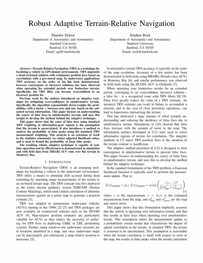
Fig. 1: Example variogram - the range and sill are thecharacteristic length over which terrain varies and the size ofthat variation.

The primary input to this model is the semi-variogram, γ(δ),which describes the spatial characteristics of the terrain. Twomain characteristics are the range and sill, shown in Figure 1,where the range is the length scale over which the terrainvaries, and the sill is the maximum amount that the terrainvaries. In uninformative terrain the variance is small and grows

much more slowly as a function of distance. Subsitituting theGaussian terrain model p(h) into Equation 15 results in

p(zzzk, h|xmk )Corr. Terrain = η1

det(Axmk

)exp

(1

2bTxm

kA−1xmkbxm

k

)(20)

where

Axmk

= HTxmk

Σ−1k,sensorHxm

k+ Σ−1

map + Σ−1terrain (21)

bxmk

= −HTxmk

Σ−1k,sensorzzzk − Σ−1

maph− Σ−1terrainµterrain (22)

In Equation 21 Hxmk

is the matrix for the observation of theterrain for the estimate xmk , Σmap is the map error (diagonalwith value σ2

map). As before, h is the map, µterrain and Σterrainare the mean and variance the terrain, zzzk and Σsensor are themeasurement and measurement noise, respectively. Both Σmapand Σterrain are of dimension n by n and Hxm

kis of dimension

n by l, where n is the total number of points in the mapand l is the number of measurements. The matrix Σsensor is ofdimension l by l.

B. TRN in Simulated Terrain

TRN runs are simulated using a short trajectory across sim-ulated terrain. The terrain patches 50m by 50m are generatedwith variograms using a Gaussian variogram model,

γ(δ) = β0 + βsill

(1− exp

(−δ2

β2range

))(23)

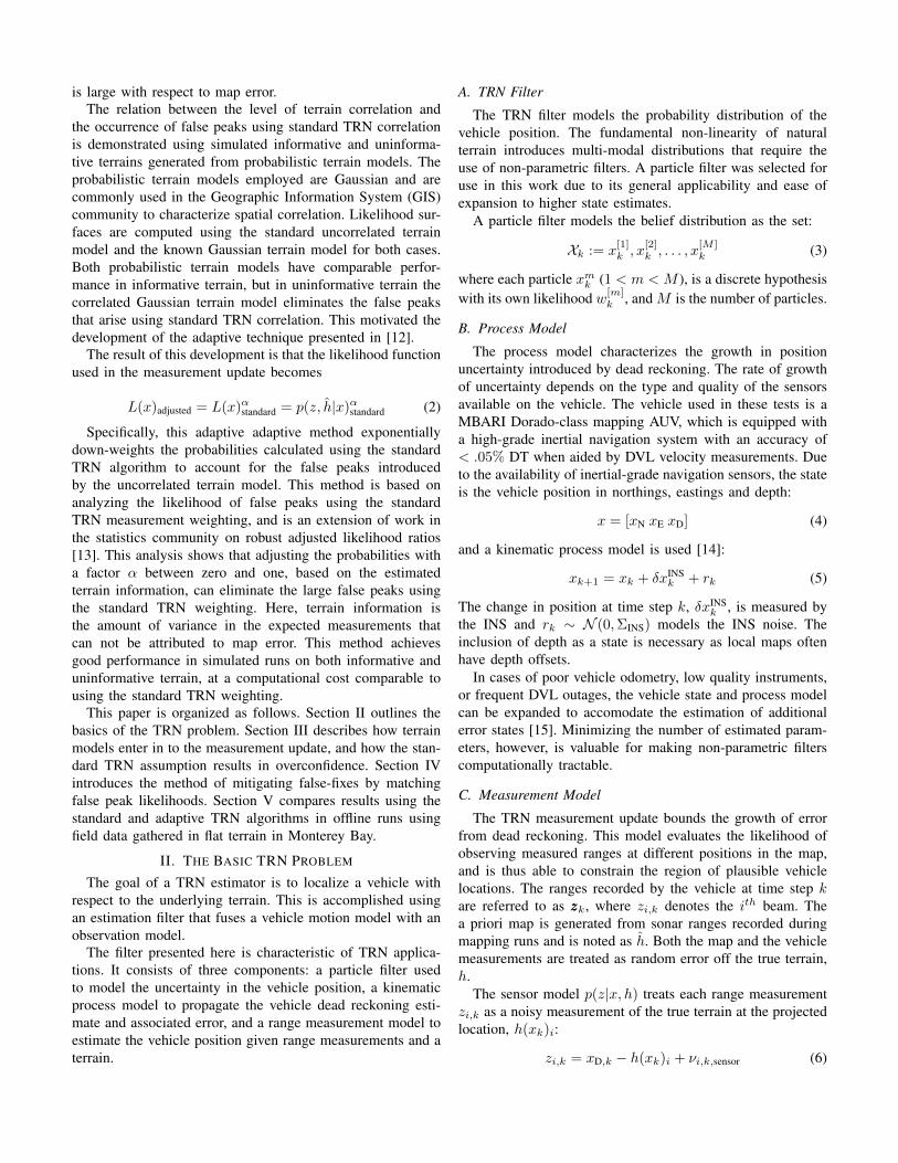
where the parameters β0, βsill and βrange control the amountof variation in the terrain and the range over which it occurs.For both cases βrange is set to 20m and β0 is set to (.01m)2,for informative terrain βsill is set to (5m)2, for uninformativeterrain βsill is set to zero. The simulated informative anduninformative terrains are shown in Figures 2 and 6.

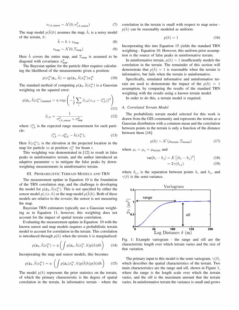
Maps of the terrain are made by adding uncorrelatedGaussian noise of variance σ2

map to all points in the terrain.Comparing the map for informative terrain in Figure 3 anduninformative terrain in Figure 7, the map noise is much moreevident when there is little terrain information.

Measured terrain profiles are simulated by adding uncorre-lated Gaussian measurement noise of variance σ2

sensor to theactual terrain profiles.

Likelihood surfaces are evaluated over a 20m by 20marea centered on the correct location at (0,0). Surfaces arecomputed using the standard weighting with p(h) = 1 fromin Equation 11 and Gaussian weighting using Equation 20with the known correlated Gaussian p(h) used to generate theterrain.

In informative terrain p(h) = 1 is a reasonable approxima-tion for the true p(h), and both weightings produce similarresults - a peak at the correct location. Results are shown inFigures 4 and 5 for the standard and Gaussian weightings,respectively.

In uninformative terrain, there is a stark difference betweenp(h) = 1 and using the correct p(h). Using p(h) = 1 resultsin a number of false peaks, shown in Figure 8, whereas the

correlated Gaussian p(h) produces a low, broad likelihoodsurface, shown in Figure 9

This motivates the development of a method for reducingflat peaks in uninformative terrain.

Fig. 2: Simulated informative terrain

Fig. 3: Map of simulated informative terrain

IV. FALSE PEAK BOUNDS AND TRN

The previous section illustrated how the terrain model usedfor standard TRN can cause issues in uninformative terrain.While one method of approaching this problem is to pursueimproved terrain models, this section introduces a differentmethod to achieve this based on bounding the size of falsepeaks.

This analysis is related to the false fix analysis by Nygrenin [11]. Nygren analyzed likelihood ratios to determine theconfidence in a PDF peak for use with a maximum-likelihoodestimator, however, in Nygrens analysis the difference betweenthe map at the two locations was assumed to be the truedifference.

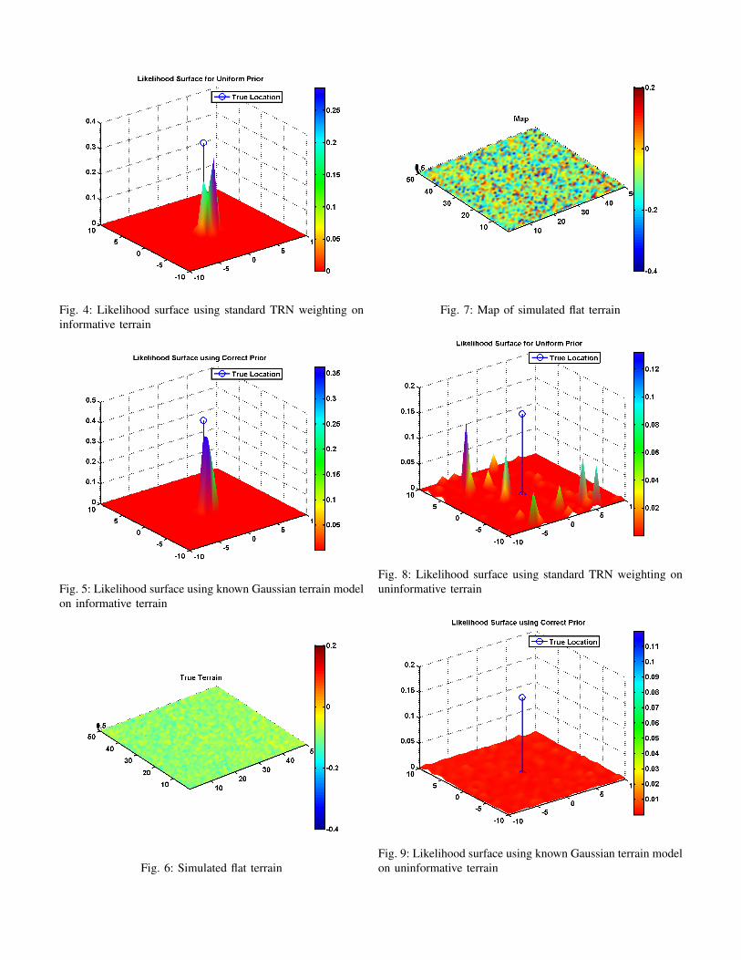
Fig. 4: Likelihood surface using standard TRN weighting oninformative terrain

Fig. 5: Likelihood surface using known Gaussian terrain modelon informative terrain

Fig. 6: Simulated flat terrain

Fig. 7: Map of simulated flat terrain

Fig. 8: Likelihood surface using standard TRN weighting onuninformative terrain

Fig. 9: Likelihood surface using known Gaussian terrain modelon uninformative terrain

A. False Peak Bounds

A false peak occurs when the data appears to provide strongsupport for the wrong hypothesis. That is, when comparing fora correct hypothesis θtrue to a false hypothesis θfalse:

L(θfalse)

L(θtrue)=p(z|θfalse)

p(z|θtrue)>> 1 (24)

For the TRN problem, the likelihood L(θ) and p(z|θ) arethe likelihood L(x) and probability p(z, h|x), respectively.While occasional support for the false hypothesis is a sta-tistical certainty, large support is unlikely when the modelsunderlying p(z|θ) are correct. Royall demonstrated in [17] thatEquation 24 can be analyzed to determine the bound on thelikelihood of false peaks, by considering

maxN

(L(θfalse)

L(θtrue)> k

)(25)

Where k is the size of the false peak, and N is the number ofmeasurements, and L(θtrue) is shorthand for p(z|θ). Maximiz-ing this as a function of N returns a bound on the probabilityof vs the size of a false peak. In [17] it was shown that whenusing correct, Gaussian models this bound is

maxN

(L(θfalse)

L(θtrue)> k

)= Φ

(−√

2 ln(k))

(26)

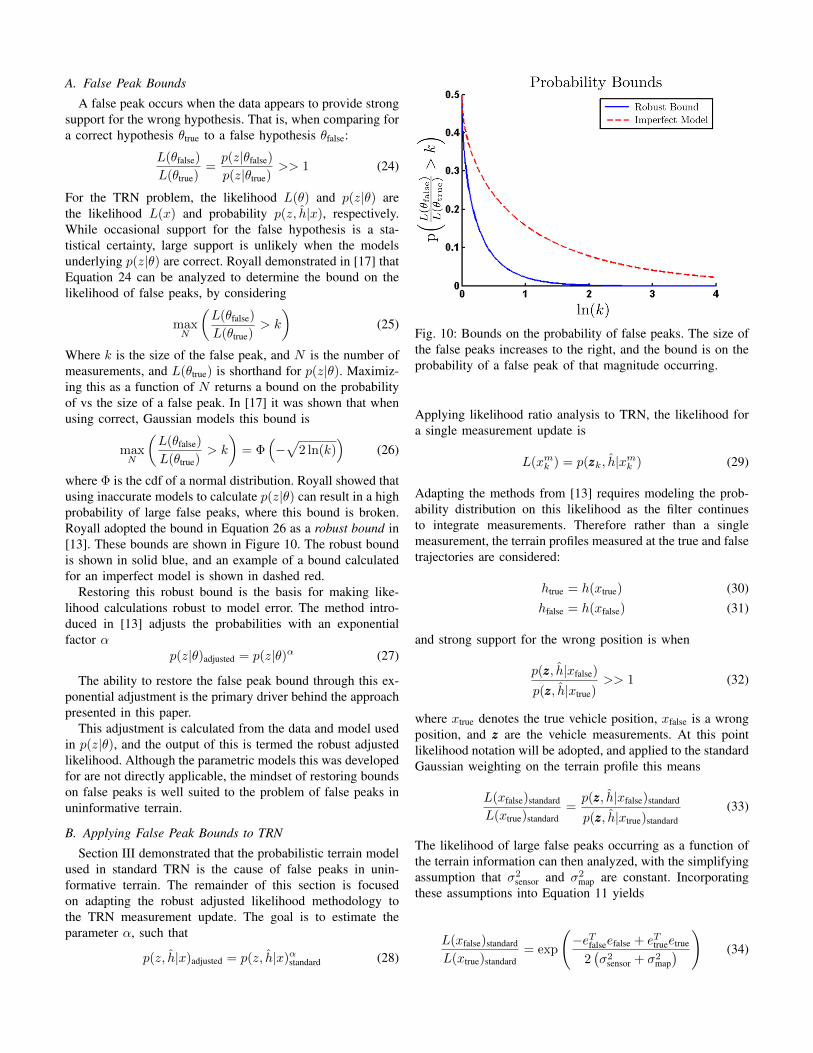
where Φ is the cdf of a normal distribution. Royall showed thatusing inaccurate models to calculate p(z|θ) can result in a highprobability of large false peaks, where this bound is broken.Royall adopted the bound in Equation 26 as a robust bound in[13]. These bounds are shown in Figure 10. The robust boundis shown in solid blue, and an example of a bound calculatedfor an imperfect model is shown in dashed red.

Restoring this robust bound is the basis for making like-lihood calculations robust to model error. The method intro-duced in [13] adjusts the probabilities with an exponentialfactor α

p(z|θ)adjusted = p(z|θ)α (27)

The ability to restore the false peak bound through this ex-ponential adjustment is the primary driver behind the approachpresented in this paper.

This adjustment is calculated from the data and model usedin p(z|θ), and the output of this is termed the robust adjustedlikelihood. Although the parametric models this was developedfor are not directly applicable, the mindset of restoring boundson false peaks is well suited to the problem of false peaks inuninformative terrain.

B. Applying False Peak Bounds to TRN

Section III demonstrated that the probabilistic terrain modelused in standard TRN is the cause of false peaks in unin-formative terrain. The remainder of this section is focusedon adapting the robust adjusted likelihood methodology tothe TRN measurement update. The goal is to estimate theparameter α, such that

p(z, h|x)adjusted = p(z, h|x)αstandard (28)

Fig. 10: Bounds on the probability of false peaks. The size ofthe false peaks increases to the right, and the bound is on theprobability of a false peak of that magnitude occurring.

Applying likelihood ratio analysis to TRN, the likelihood fora single measurement update is

L(xmk ) = p(zzzk, h|xmk ) (29)

Adapting the methods from [13] requires modeling the prob-ability distribution on this likelihood as the filter continuesto integrate measurements. Therefore rather than a singlemeasurement, the terrain profiles measured at the true and falsetrajectories are considered:

htrue = h(xtrue) (30)hfalse = h(xfalse) (31)

and strong support for the wrong position is when

p(zzz, h|xfalse)

p(zzz, h|xtrue)>> 1 (32)

where xtrue denotes the true vehicle position, xfalse is a wrongposition, and zzz are the vehicle measurements. At this pointlikelihood notation will be adopted, and applied to the standardGaussian weighting on the terrain profile this means

L(xfalse)standard

L(xtrue)standard=p(zzz, h|xfalse)standard

p(zzz, h|xtrue)standard(33)

The likelihood of large false peaks occurring as a function ofthe terrain information can then analyzed, with the simplifyingassumption that σ2

sensor and σ2map are constant. Incorporating

these assumptions into Equation 11 yields

L(xfalse)standard

L(xtrue)standard= exp

(−eTfalseefalse + eTtrueetrue

2(σ2

sensor + σ2map

) )(34)

where

etrue = z − ztrue (35)

= (xD,true − htrue + νsensor)− (xD,true − htrue) (36)= (xD,true − htrue + νsensor)− (xD,true − htrue − νmap,true)

(37)= νsensor − νmap,true (38)

At the false location,

efalse = z − zfalse (39)

= (xD,true − htrue + νsensor)− (xD,false − hfalse) (40)= (xD,true − htrue + νsensor)− (xD,false − hfalse − νmap,false)

(41)= νsensor + δt-f − νmap,false (42)

where the difference between the expected measurements ofthe true and false trajectories is δt-f

δt-f = (xD,true − xD,false) + (htrue − hfalse) (43)

Equations 35 and 39 can be interpreted as follows: for the truetrajectory the expected difference between the measurementsand the map is the sum of the noise in the measurementsand the map, whereas at the false location there is also acontribution from the difference between the terrain profilesand error in the depth estimate. In the case of known depth,δt-f is the difference between terrain profiles, and as such isreferred to as the terrain information. With these models, thefalse peak likelihood using Equation 34 can be evaluated asa function of the map noise, sensor noise, and the differenceδt-f.

p

(L(xfalse)standard

L(xtrue)standard> k

)= f

(δt-f, σ

2map, σ

2terrain, k

)(44)

Although the analysis can be done with any δt-f profiledifference, it is the sum of the squared difference, δTt-fδt-f thatenters into the equation. This term is therefore modeled as

δTt-fδt-f ∼ Nδ2rms (45)

Where δrms is used to characterize the RMS terrain profiledifference. The pdf of the likelihoood ratio can thus be writtenas a log-normal distribution,

p

(L(xfalse)standard

L(xtrue)standard

)∼ lnN

(µLR, σ

2LR

)(46)

where the terms µLR and σ2LR are a function of δrms,

σ2map,σ2

terrain, and the profile length N .

µLR =−Nδ2rms

2(σ2

sensor + σ2map

) (47)

σ2LR =

N((σ2

sensor + σ2map

) (δ2rms + σ2

map

)+ σ2

sensorσ2map

)(σ2

sensor + σ2map

)2 (48)

With this log-normal distribution, a more negative mean indi-cates a lower likelihood of a false peak, but a larger standarddeviation results in a larger spread in possible weightings and

higher likelihood of false peaks. A simple example is the casefor flat terrain - as there is no information in the terrain, themean stays at zero (eg, the true location is indistinguishablefrom the false location), however because of the growingvariance there is will be a high likelihood of strong evidence infavor of either location. Thus, the likelihood of false peaks isdetermined by the growth of the mean relative to the standarddeviation.

Calculating the likelihood of a mis-weighting using thestandard TRN formula is therefore done with the cumulativedistribution of a normal variable. For a mis-weighting greaterthan k, that returns:

p

(L(xfalse)standard

L(xtrue)standard> k

)= Φ

(µLR − ln (k)

σLR

)(49)

The bound on the likelihood of a false peak of size k iscalculated by maximizing this probability. As δrms, σ2

map andσ2

terrain are fixed, this is with respect to N , and is

maxN

p

(L(xfalse)standard

L(xtrue)standard> k

)= Φ

(−√aLR

bLR

√2 ln (k)

)(50)

where

aLR = δ2rms (51)

bLR =

(σ2

sensor + σ2map

) (δ2rms + σ2

map

)+ σ2

sensorσ2map

σ2sensor + σ2

map(52)

and aLR and bLR are dependent only on the terrain information,map and sensor error.

Examining this equation shows two important features. Thefirst is that, in the case where the map error is small withrespect to the terrain information, σ2

map is small with respectto δ2rms, aLR ≈ bLR and the bound on false peaks matches therobust bound. The second is that the robust bound will besignificantly broken in flat terrain, when σ2

map is large withrespect to δ2rms. This makes aLR small compared to bLR, andconsequently the likelihood of false peaks will be much higher.The broken bound shown in Figure 10 is for the case whereσ2m,σ2

m are 1 and δ2rms is 0.5.The general conclusion is that the lower the amount of

terrain information relative to map error, the further to theright the false peak bound is pushed. That is, the likelihoodof large false peaks is increased. This supports the simulationresults from Section III-B, where there were many large peaksin uninformative terrain.

The robust bound on false peaks can be restored in unin-formative terrain through the parameter α, which changes themean and variance of the likelihood ratio. Noting the adjustedlikelihood ratio as

L(x)adjusted = L(x)αstandard = p(zzz, h|x)αstandard (53)

the mean and variance of the log-normal likelihood ratiobecome

µLR, adjusted = αµLR (54)

σ2LR, adjusted = α2σ2

LR (55)

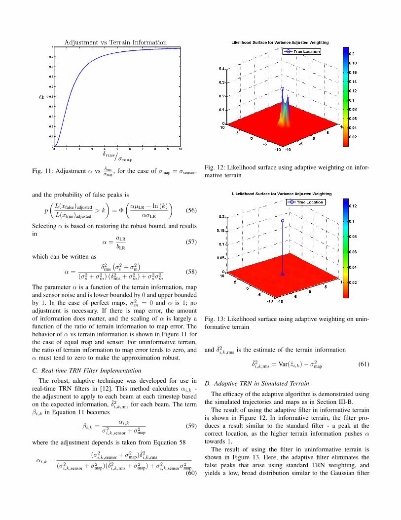
Fig. 11: Adjustment α vs δrmsσmap

, for the case of σmap = σsensor.

and the probability of false peaks is

p

(L(xfalse)adjusted

L(xtrue)adjusted> k

)= Φ

(αµLR − ln (k)

ασLR

)(56)

Selecting α is based on restoring the robust bound, and resultsin

α =aLR

bLR(57)

which can be written as

α =δ2rms

(σ2

s + σ2m

)(σ2s + σ2

m) (δ2rms + σ2m) + σ2

sσ2m

(58)

The parameter α is a function of the terrain information, mapand sensor noise and is lower bounded by 0 and upper boundedby 1. In the case of perfect maps, σ2

m = 0 and α is 1; noadjustment is necessary. If there is map error, the amountof information does matter, and the scaling of α is largely afunction of the ratio of terrain information to map error. Thebehavior of α vs terrain information is shown in Figure 11 forthe case of equal map and sensor. For uninformative terrain,the ratio of terrain information to map error tends to zero, andα must tend to zero to make the approximation robust.

C. Real-time TRN Filter Implementation

The robust, adaptive technique was developed for use inreal-time TRN filters in [12]. This method calculates αi,k -the adjustment to apply to each beam at each timestep basedon the expected information, δ2i,k,rms for each beam. The termβi,k in Equation 11 becomes

βi,k =αi,k

σ2i,k,sensor + σ2

map(59)

where the adjustment depends is taken from Equation 58

αi,k =(σ2i,k,sensor + σ2

map)δ2i,k,rms

(σ2i,k,sensor + σ2

map)(δ2i,k,rms + σ2map) + σ2

i,k,sensorσ2map(60)

Fig. 12: Likelihood surface using adaptive weighting on infor-mative terrain

Fig. 13: Likelihood surface using adaptive weighting on unin-formative terrain

and δ2i,k,rms is the estimate of the terrain information

δ2i,k,rms = Var(zi,k)− σ2map (61)

D. Adaptive TRN in Simulated Terrain

The efficacy of the adaptive algorithm is demonstrated usingthe simulated trajectories and maps as in Section III-B.

The result of using the adaptive filter in informative terrainis shown in Figure 12. In informative terrain, the filter pro-duces a result similar to the standard filter - a peak at thecorrect location, as the higher terrain information pushes αtowards 1.

The result of using the filter in uninformative terrain isshown in Figure 13. Here, the adaptive filter eliminates thefalse peaks that arise using standard TRN weighting, andyields a low, broad distribution similar to the Gaussian filter

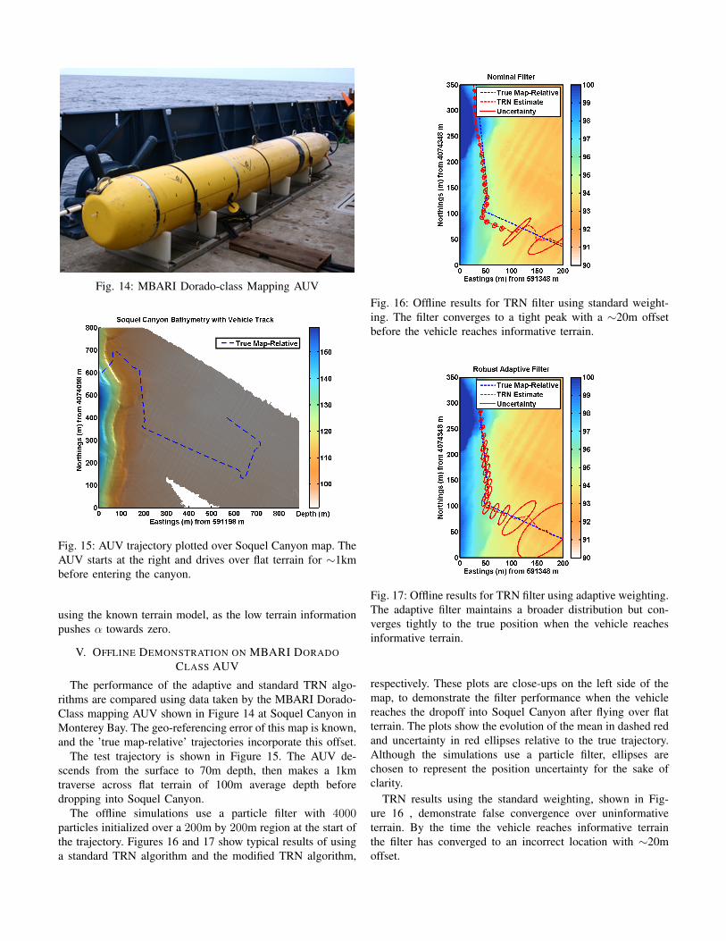
Fig. 14: MBARI Dorado-class Mapping AUV

Fig. 15: AUV trajectory plotted over Soquel Canyon map. TheAUV starts at the right and drives over flat terrain for ∼1kmbefore entering the canyon.

using the known terrain model, as the low terrain informationpushes α towards zero.

V. OFFLINE DEMONSTRATION ON MBARI DORADOCLASS AUV

The performance of the adaptive and standard TRN algo-rithms are compared using data taken by the MBARI Dorado-Class mapping AUV shown in Figure 14 at Soquel Canyon inMonterey Bay. The geo-referencing error of this map is known,and the ’true map-relative’ trajectories incorporate this offset.

The test trajectory is shown in Figure 15. The AUV de-scends from the surface to 70m depth, then makes a 1kmtraverse across flat terrain of 100m average depth beforedropping into Soquel Canyon.

The offline simulations use a particle filter with 4000particles initialized over a 200m by 200m region at the start ofthe trajectory. Figures 16 and 17 show typical results of usinga standard TRN algorithm and the modified TRN algorithm,

Fig. 16: Offline results for TRN filter using standard weight-ing. The filter converges to a tight peak with a ∼20m offsetbefore the vehicle reaches informative terrain.

Fig. 17: Offline results for TRN filter using adaptive weighting.The adaptive filter maintains a broader distribution but con-verges tightly to the true position when the vehicle reachesinformative terrain.

respectively. These plots are close-ups on the left side of themap, to demonstrate the filter performance when the vehiclereaches the dropoff into Soquel Canyon after flying over flatterrain. The plots show the evolution of the mean in dashed redand uncertainty in red ellipses relative to the true trajectory.Although the simulations use a particle filter, ellipses arechosen to represent the position uncertainty for the sake ofclarity.

TRN results using the standard weighting, shown in Fig-ure 16 , demonstrate false convergence over uninformativeterrain. By the time the vehicle reaches informative terrainthe filter has converged to an incorrect location with ∼20moffset.

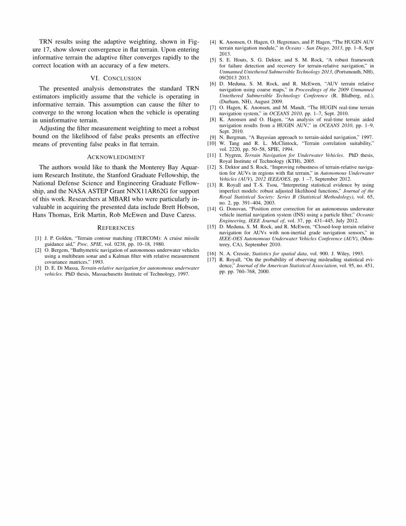
TRN results using the adaptive weighting, shown in Fig-ure 17, show slower convergence in flat terrain. Upon enteringinformative terrain the adaptive filter converges rapidly to thecorrect location with an accuracy of a few meters.

VI. CONCLUSION

The presented analysis demonstrates the standard TRNestimators implicitly assume that the vehicle is operating ininformative terrain. This assumption can cause the filter toconverge to the wrong location when the vehicle is operatingin uninformative terrain.

Adjusting the filter measurement weighting to meet a robustbound on the likelihood of false peaks presents an effectivemeans of preventing false peaks in flat terrain.

ACKNOWLEDGMENT

The authors would like to thank the Monterey Bay Aquar-ium Research Institute, the Stanford Graduate Fellowship, theNational Defense Science and Engineering Graduate Fellow-ship, and the NASA ASTEP Grant NNX11AR62G for supportof this work. Researchers at MBARI who were particularly in-valuable in acquiring the presented data include Brett Hobson,Hans Thomas, Erik Martin, Rob McEwen and Dave Caress.

REFERENCES

[1] J. P. Golden, “Terrain contour matching (TERCOM): A cruise missileguidance aid,” Proc. SPIE, vol. 0238, pp. 10–18, 1980.

[2] O. Bergem, “Bathymetric navigation of autonomous underwater vehiclesusing a multibeam sonar and a Kalman filter with relative measurementcovariance matrices,” 1993.

[3] D. E. Di Massa, Terrain-relative navigation for autonomous underwatervehicles. PhD thesis, Massachusetts Institute of Technology, 1997.

[4] K. Anonsen, O. Hagen, O. Hegrenaes, and P. Hagen, “The HUGIN AUVterrain navigation module,” in Oceans - San Diego, 2013, pp. 1–8, Sept2013.

[5] S. E. Houts, S. G. Dektor, and S. M. Rock, “A robust frameworkfor failure detection and recovery for terrain-relative navigation,” inUnmanned Untethered Submersible Technology 2013, (Portsmouth, NH),09/2013 2013.

[6] D. Meduna, S. M. Rock, and R. McEwen, “AUV terrain relativenavigation using coarse maps,” in Proceedings of the 2009 UnmannedUntethered Submersible Technology Conference (R. Blidberg, ed.),(Durham, NH), August 2009.

[7] O. Hagen, K. Anonsen, and M. Mandt, “The HUGIN real-time terrainnavigation system,” in OCEANS 2010, pp. 1–7, Sept. 2010.

[8] K. Anonsen and O. Hagen, “An analysis of real-time terrain aidednavigation results from a HUGIN AUV,” in OCEANS 2010, pp. 1–9,Sept. 2010.

[9] N. Bergman, “A Bayesian approach to terrain-aided navigation,” 1997.[10] W. Tang and R. L. McClintock, “Terrain correlation suitability,”

vol. 2220, pp. 50–58, SPIE, 1994.[11] I. Nygren, Terrain Navigation for Underwater Vehicles. PhD thesis,

Royal Institute of Technology (KTH), 2005.[12] S. Dektor and S. Rock, “Improving robustness of terrain-relative naviga-

tion for AUVs in regions with flat terrain,” in Autonomous UnderwaterVehicles (AUV), 2012 IEEE/OES, pp. 1 –7, September 2012.

[13] R. Royall and T.-S. Tsou, “Interpreting statistical evidence by usingimperfect models: robust adjusted likelihood functions,” Journal of theRoyal Statistical Society: Series B (Statistical Methodology), vol. 65,no. 2, pp. 391–404, 2003.

[14] G. Donovan, “Position error correction for an autonomous underwatervehicle inertial navigation system (INS) using a particle filter,” OceanicEngineering, IEEE Journal of, vol. 37, pp. 431–445, July 2012.

[15] D. Meduna, S. M. Rock, and R. McEwen, “Closed-loop terrain relativenavigation for AUVs with non-inertial grade navigation sensors,” inIEEE-OES Autonomous Underwater Vehicles Conference (AUV), (Mon-terey, CA), September 2010.

[16] N. A. Cressie, Statistics for spatial data, vol. 900. J. Wiley, 1993.[17] R. Royall, “On the probability of observing misleading statistical evi-

dence,” Journal of the American Statistical Association, vol. 95, no. 451,pp. pp. 760–768, 2000.