Robust 3D Hand Tracking for Human Computer Interaction

Victor Adrian PrisacariuDepartment of Engineering Science

University of Oxfordvictor@robots.ox.ac.uk

Ian ReidDepartment of Engineering Science

University of Oxfordian@robots.ox.ac.uk

Abstract— We propose a system for human computer interac-tion via 3D hand movements, based on a combination of visualtracking and a cheap, off-the-shelf, accelerometer. We use a3D model and region based tracker, resulting in robustnessto variations in illumination, motion blur and occlusions. Atthe same time the accelerometer allows us to deal with themultimodality in the silhouette to pose function. We synchronisethe accelerometer and tracker online, by casting the calibrationproblem as a maximum covariance problem, which we thensolve probabilistically. We show the effectiveness of our solutionwith multiple real-world tests and demonstration scenarios.

I. INTRODUCTION

With the advent of processing power and the internet, thecomputer has become a gaming and media hub and partof the centre of our social life. Still, interaction with it isvery limited to mouse and keyboard. This paper describesa natural and intuitive way of interacting with a virtualenvironment, by employing a vision and inertial sensor-basedsystem, to recover the 3D non-articulated pose of a humanhand in real time, while still creating a cost effective system.

Fast and reliable hand tracking has usually been achievedusing glove-based approaches. For example, the ShapeHanddata glove [8] uses accelerometers, gyroscopes and flexsensors, while in [15] the authors use a specially colouredglove (but no sensors) to obtain the full 3D articulatedpose of a hand. Both these systems show very good results.However the ShapeHand data glove is both intrusive andexpensive, and the authors in [15] limit themselves to clean,clutter-free environments.

Our method combines a vision based 3D tracker, similarto the one presented in [11], with a single off-the-shelfaccelerometer. This gives it the following significant advan-tages over previous hand tracking work: (i) it works in realtime and in real-world environments (cluttered and with largeamounts of motion blur and occlusions) and (ii) it is muchless intrusive when compared to glove-based approaches.

Vision based 3D hand tracking can be split into model-based and appearance-based tracking [10]. A model-basedtechnique has a number of important elements: a 3D model,a set of image features, an error function and a non-linearoptimisation algorithm. At every frame the set of features isextracted from the image and an error function is minimised.This energy function relates the pose of the 3D model to thefeatures extracted from the image. The features may be sim-ple (edges, points) or complex (3D depth information). Mostoften edges and colour are combined to form a silhouette.The 3D model may be anything between a coarse geometricmodel and a detailed 3D reconstruction (including shading

and texture information) of the user’s hand. For example[12] uses a model built only from quadratics while in [4]both texture and lighting are used. To form the error functionthe 3D model may be projected down or the image featuresmay be projected up. The minimisation may lead to one orto several hypotheses. Finally sometimes the hand motiondynamics are used, therefore predicting the pose of the nextframe from the poses at the current frame and previousframes.

Appearance-based algorithms propose to learn a directmapping between image features and pose, so only twosteps are required when a new frame is presented: extractthe image features and obtain the pose from the feature–pose mapping. These methods need no initialisation and are(theoretically) faster, because most of the processing effort isput into offline training, rather than in the online phase. Themapping between feature and pose can either be learnt insidea database in [1], by using a tree-based filter in [12] or viaa Relevance Vector Machine in [3]. These methods, whilemaybe producing good results in a controlled environmentwhere the segmentation is very good, do not perform wellin real-world scenarios.

Our visual tracker is model and region based: we usesimple 3D meshes as models (so no texture or lightinginformation) and a region based energy function. This energyfunction uses the implicit representation of the contour ofthe projection of the known 3D model, by embedding itinside a level set function. We maximise the posterior per-pixel probability of foreground and background membershipas a function of pose, directly, bypassing any separatesegmentation phase. We represent the region statistics byvariable bin size, colour histograms and adapt these online.Since we are using only the silhouette of the projection, theenergy function will be multimodal. To help deal with theambiguities, we place an accelerometer on the hand.

The remainder of this article is structured as follows: inSection II we present the 3D tracker, in Section IV wedetail the way in which we extract the orientation from theaccelerometer and correlate it with the tracker and in SectionV we show various results. We conclude in Section VI.

II. 3D TRACKER

This section presents the details of our 3D tracker, similarto the one published in [11]. Here we review that work,then in subsections II-D, II-E and II-F we describe severalimprovements. We first set up the notation. We then show our

3D model and detail the tracking algorithm and the regionstatistics.

A. Notation

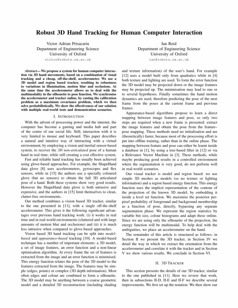
Fig. 1. Notation – the contour around the visible part of the 3D model(green) and its corresponding projection C (red), the foreground regionΩ f and the background region Ωb, a 2D point x on the contour and itscorresponding 3D point in the object coordinate frame, X

Let the image be denoted by I, and the image domain byΩ⊂R2 with the area element dΩ. An image pixel x = [x,y]has a corresponding image value I(x)= y (in our experimentsa RGB value), a corresponding 3D point X = [X ,Y,Z]T =RX0 +T ∈ R3 in the camera coordinate frame and a pointX0 = [X0,Y0,Z0]

T ∈R3 in the object coordinate frame. R andT are the rotation matrix and translation vector representingthe unknown pose and are parametrised by 7 parameters (4for rotation and 3 for translation), denoted by λi.

We assume the intrinsic parameters of the camera to beknown. Let ( fu, fv) be the focal length and (uo,vo) theprincipal point of the camera.

The contour around the visible part of the object in 3D(marked with green in Figure 1) projects to the contour Cin the image (marked with red). We embed C in the zerolevel-set function Φ(x). The contour C also segments theimage into two disjoint regions: foreground denoted by Ω fand background denoted by Ωb. Each region has its ownstatistical appearance model P(y|M),M ∈ M f ,Mb.

Finally, by He(x) we denote the smoothed Heaviside stepfunction and by δe(x) the smoothed Dirac delta function.

B. 3D Model

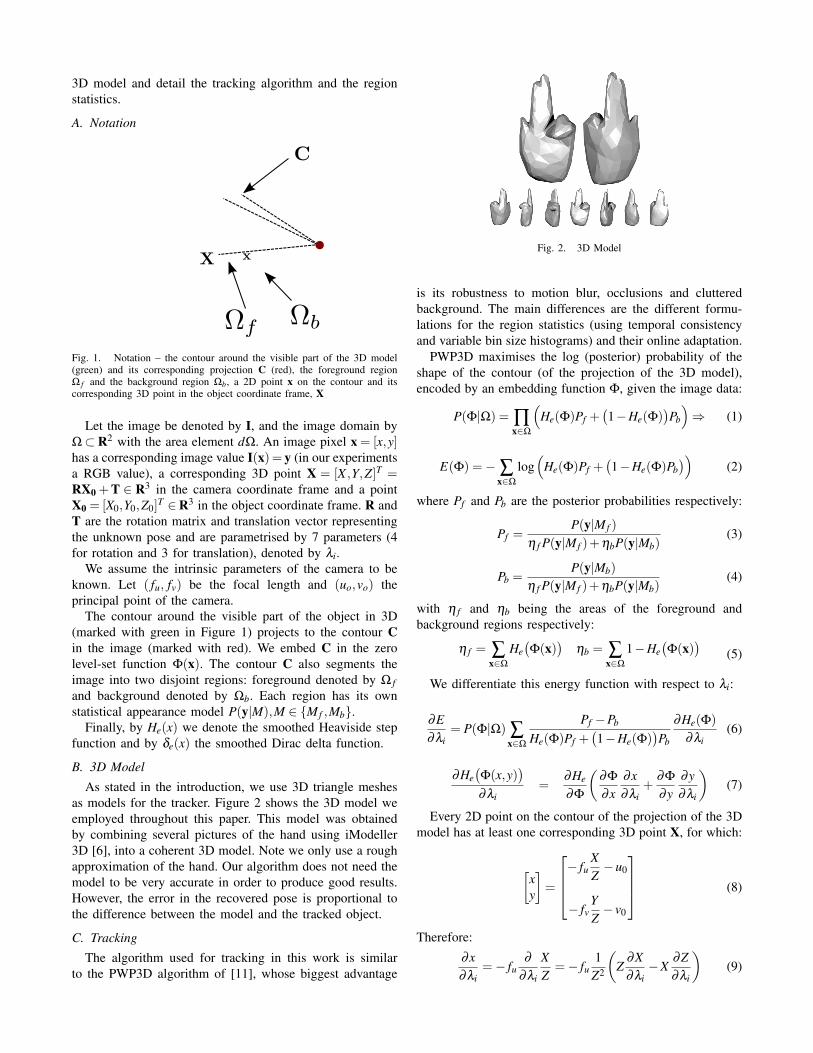
As stated in the introduction, we use 3D triangle meshesas models for the tracker. Figure 2 shows the 3D model weemployed throughout this paper. This model was obtainedby combining several pictures of the hand using iModeller3D [6], into a coherent 3D model. Note we only use a roughapproximation of the hand. Our algorithm does not need themodel to be very accurate in order to produce good results.However, the error in the recovered pose is proportional tothe difference between the model and the tracked object.

C. Tracking

The algorithm used for tracking in this work is similarto the PWP3D algorithm of [11], whose biggest advantage

Fig. 2. 3D Model

is its robustness to motion blur, occlusions and clutteredbackground. The main differences are the different formu-lations for the region statistics (using temporal consistencyand variable bin size histograms) and their online adaptation.

PWP3D maximises the log (posterior) probability of theshape of the contour (of the projection of the 3D model),encoded by an embedding function Φ, given the image data:

P(Φ|Ω) = ∏x∈Ω

(He(Φ)Pf +

(1−He(Φ)

)Pb

)⇒ (1)

E(Φ) =− ∑x∈Ω

log(

He(Φ)Pf +(1−He(Φ)Pb

))(2)

where Pf and Pb are the posterior probabilities respectively:

Pf =P(y|M f )

η f P(y|M f )+ηbP(y|Mb)(3)

Pb =P(y|Mb)

η f P(y|M f )+ηbP(y|Mb)(4)

with η f and ηb being the areas of the foreground andbackground regions respectively:

η f = ∑x∈Ω

He(Φ(x)

)ηb = ∑

x∈Ω

1−He(Φ(x)

)(5)

We differentiate this energy function with respect to λi:

∂E∂λi

= P(Φ|Ω) ∑x∈Ω

Pf −Pb

He(Φ)Pf +(1−He(Φ)

)Pb

∂He(Φ)

∂λi(6)

∂He(Φ(x,y)

)∂λi

=∂He

∂Φ

(∂Φ

∂x∂x∂λi

+∂Φ

∂y∂y∂λi

)(7)

Every 2D point on the contour of the projection of the 3Dmodel has at least one corresponding 3D point X, for which:

[xy

]=

− fu

XZ−u0

− fvYZ− v0

(8)

Therefore:

∂x∂λi

=− fu∂

∂λi

XZ=− fu

1Z2

(Z

∂X∂λi−X

∂Z∂λi

)(9)

The differential ∂y∂λi

is analogue to ∂x∂λi

while ∂X∂λi

, ∂Y∂λi

and∂Z∂λi

follow trivially by differentiating X = RX0 + T withrespect to λi. For more details the reader is refereed to [11].

D. Temporal Consistency

The probability of a pixel being foreground or backgroundshould not change instantly i.e. if a pixel was foreground attime t− 1, the probability of it being foreground at time tshould be higher than the probability of it being background.This can be written formally, using a recursive Bayes filter:

P(Mtj|Yt) =

P(yt |Mtj,Yt−1)P(Mt

j|Yt−1)

P(yt |Yt−1)(10)

where M j, j ∈ f ,b is the foreground/background model,yt the value of pixel y at time t and Yt = [yt ,yt−1, . . .] thevalues of pixel y up to time t.

Assuming conditional independence we can write:

P(Mtj|Yt) =

P(yt |Mtj)P(M

tj|Yt−1)

P(yt |Yt−1)=

=P(yt |Mt

j)∑i∈ f ,b(

p(Mti |M

t−1i )p(Mt−1

i |Yt−1))

P(yt |Yt−1)(11)

where:

P(yt |Yt−1) = ∑i∈ f ,b

P(yt |Mti )P(M

ti |Yt−1) (12)

The recursion is initialised by P(M0) = P(M j).To estimate the per pixel values for P(Mt

f |Mt−1f ) and

P(Mtb|M

t−1b ) we define two classes of pixels γ f and γb rep-

resenting the unchanged (between the previous and currentframe) foreground and background pixels respectively. Thefollowing posteriors can be obtained:

P(Mtf |Mt−1

f ) =P(γ f |yt ,yt−1) = P(yt ,yt−1|γ f )P(γ f ) =

=P(yt |M f )P(yt−1|M f )P(γ f )

P(Mtb|Mt−1

b ) =P(γb|yt ,yt−1) = P(yt ,yt−1|γb)P(γb) =

=P(yt |Mb)P(yt−1|Mb)P(γb)

(13)

with

P(γ f ) =ζ f

ζP(ζb) =

ζb

ζ(14)

where ζ is the total number of pixels in the image, ζi,i ∈ f ,b is the number of pixels that didn’t change typebetween the previous and current frames i.e. had proba-bility of foreground/background bigger than that of back-ground/foreground and the pixel colour didn’t change bymore than a fixed threshold.

Here we only consider Yt = yt , which means that thecurrent value the foreground/background posterior dependsonly on the value at the previous time step.

E. Variable Bin Size Histograms

In [11] and [2] the authors use a standard appearancemodel consisting of two 32 bin histograms (one for fore-ground and one for background).

We have empirically observed that the dynamic responseof the sort of consumer grade webcams is such that brightcolours will have a higher variance to changing lightingconditions than dark colours. Standard histograms use thesame number of bins for both bright and dark colours, whichleads to undersampling for dark colours and oversamplingfor bright colours. Put differently, if we build the histogramof an object of bright constant colour, under uneven lightingconditions, rather than having a single peak, the histogramwill tend to flatten. If the object is dark we will end up havinga single peak inside the histogram, when it should actuallybe flatter. One solution to this problem would be to separatebrightness from colour, by using a different colour space(HSV, HSL, etc.). This would imply an extra processing stepand these colour spaces have singularities at dark colours.

Our solution is to keep using the RGB colour space, butvary the number of bins in the histogram, according to thebrightness of the pixel: bright colours will use fewer binswhile dark colours use more bins. In our implementation weuse 4 histograms (of 8, 16, 32, 64 bins per channel).

F. Online Adaptation

In [11] the authors updated the histogram only when theminimisation of the energy function had converged. Thisdoes not guarantee that the histograms will not be corrupted,because the minimisation of the energy function might haveconverged to an incorrect pose. Here we use the distancetransform as a measure of contour uncertainty: points thatare far from the contour, and inside the projection will mostlikely be foreground, while pixels far from the contour andoutside the projection will most likely be background. Weevaluate the distance transform in a band around the contourso we update the foreground histogram only with the pixelsoutside the band but inside the contour and the backgroundone with pixels outside the band and outside the contour.This might mean that we do not update with some pixelsthat actually are foreground / background but it allows us touse much higher adaptation rates while still ensuring stabletracking. In [11] the adaptation rate was usually less than 1%.Here we can easily go as high as 5% learning rate without thehistograms getting corrupted. This allows more rapid changesin appearance which in turn produces more reliable tracking.

III. IMPLEMENTATION AND TIMINGS

To be useful in real-world applications, a 3D hand trackerhas to work in real time. To this end we used a highly-parallel GPU implementation similar to that of [11]. Theenergy function from Equation 2 is minimised using gradientdescent, for expedience and ease of implementation. Eachgradient descent iteration proceeds as follows:• The 3D model is rendered using the current estimate of

the pose.

• The contour of the rendering and its exact signeddistance transform are computed.

• The partial derivatives of the energy function withrespect to the pose parameters are calculated.

• A step change is made, in the direction of the gradient.The step size is fixed.

In [11] the authors parallelised everything except the 3Drendering step. This ended up being the bottleneck in theirimplementation, because the rendering and transfer to theGPU operations took as much as the rest of the processing(distance transform and energy function evaluation). AnOpenGL based implementation would have actually beenslower (at least for models with few triangles) [11].

Here we developed our own NVIDIA CUDA-based 3Drendering engine. We chose to use a separate thread for eachtriangle in the model. For the ZBuffer implementation we useglobal memory write atomic operations to avoid any possibleread-write-modify hazard. As a result we are able to achievespeeds of 2-3ms per iteration (compared to 4-6 in [11]).Reliable tracking can be done at 15-20 frames per secondwhen running a fixed number of iterations. Convergence isusually faster than the fixed number of iterations so the speedincreases to 20-25 frames per second when checking forconvergence. In this paper we used a NVIDIA GTX 285video card and an Intel Xeon E5420 CPU.

IV. ACCELEROMETER

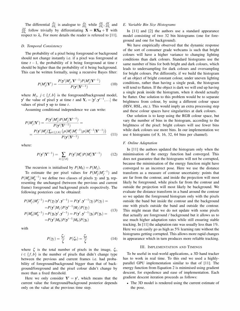
Fig. 3. Silhouette - Pose ambiguities

The function mapping silhouette to pose is multimodal:very different poses will end up generating the very similarsilhouettes, as shown in Figure 3. One solution to overcomethis problem would be to consider multiple hypotheses atevery frame (i.e. use a particle filter). This would makereal time performance difficult to achieve. Our solution isto augment the 3D tracker with data from a simple off-the-shelf accelerometer, mounted on the hand. In this section wepresent our method of extracting data from the accelerometerand of calibrating the accelerometer and tracker.

A. Extracting Hand Orientation from the Accelerometer

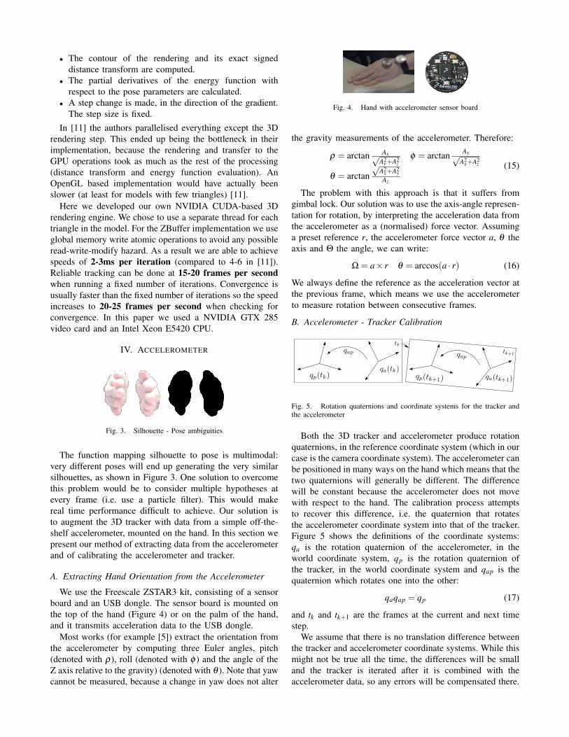
We use the Freescale ZSTAR3 kit, consisting of a sensorboard and an USB dongle. The sensor board is mounted onthe top of the hand (Figure 4) or on the palm of the hand,and it transmits acceleration data to the USB dongle.

Most works (for example [5]) extract the orientation fromthe accelerometer by computing three Euler angles, pitch(denoted with ρ), roll (denoted with φ ) and the angle of theZ axis relative to the gravity) (denoted with θ ). Note that yawcannot be measured, because a change in yaw does not alter

Fig. 4. Hand with accelerometer sensor board

the gravity measurements of the accelerometer. Therefore:

ρ = arctan Ax√A2

y+A2z

φ = arctan Ay√A2

x+A2z

θ = arctan√

A2x+A2

yAz

(15)

The problem with this approach is that it suffers fromgimbal lock. Our solution was to use the axis-angle represen-tation for rotation, by interpreting the acceleration data fromthe accelerometer as a (normalised) force vector. Assuminga preset reference r, the accelerometer force vector a, θ theaxis and Θ the angle, we can write:

Ω = a× r θ = arccos(a · r) (16)

We always define the reference as the acceleration vector atthe previous frame, which means we use the accelerometerto measure rotation between consecutive frames.

B. Accelerometer - Tracker Calibration

Fig. 5. Rotation quaternions and coordinate systems for the tracker andthe accelerometer

Both the 3D tracker and accelerometer produce rotationquaternions, in the reference coordinate system (which in ourcase is the camera coordinate system). The accelerometer canbe positioned in many ways on the hand which means that thetwo quaternions will generally be different. The differencewill be constant because the accelerometer does not movewith respect to the hand. The calibration process attemptsto recover this difference, i.e. the quaternion that rotatesthe accelerometer coordinate system into that of the tracker.Figure 5 shows the definitions of the coordinate systems:qa is the rotation quaternion of the accelerometer, in theworld coordinate system, qp is the rotation quaternion ofthe tracker, in the world coordinate system and qap is thequaternion which rotates one into the other:

qaqap = qp (17)

and tk and tk+1 are the frames at the current and next timestep.

We assume that there is no translation difference betweenthe tracker and accelerometer coordinate systems. While thismight not be true all the time, the differences will be smalland the tracker is iterated after it is combined with theaccelerometer data, so any errors will be compensated there.

Several visual-inertial calibration methods exist. Generallythis problem is solved as one of linear or nonlinear leastsquares [7], [9]. For example in [9] the authors start fromthe fact that qap should be constant and minimise:

qpa = argmaxqqT( t

∑i=1

QT∆qa(t)Q∆qp(t)

)q (18)

where qpa = q−1ap , Q and Q are the matrix representations of

∆qa and ∆qp, and:

∆qp = q−1p (t1)qp(t2) ∆qa = q−1

a (t1)qa(t2) (19)

Our solution assumes the user moves the hand in apredefined pattern (up, down, left, right), to pass through theentire range of valid accelerometer values. We compute qapat every frame and then the eigenvectors of the covariancematrix built by stacking together all the qap values. Sinceeigenvectors norm to 1, all eigenvectors will be valid quater-nions. The calibrated quaternion, relating qp to qa, is then theeigenvector with the maximum eigenvalue i.e. the one thatmaximises the variance among all the values of qap. Thisprocess could also be seen as running Principal ComponentAnalysis (PCA) on the quaternion dataset.

Least squares based methods and PCA assume all datapoints to be i.i.d. and corrupted by i.i.d. noise. However thenoise in our case is not i.i.d. A quaternion describes a singlerotation, making the quaternion parameters interlinked. Thenoise in the quaternion parameters can therefore be approx-imated more accurately by spherical noise. Therefore in thiswork, rather than running PCA on the quaternion dataset werun Probabilistic PCA [14], which considers noise as beingspherical Gaussian.

C. Accelerometer - Tracker Integration

Ideally we would operate with visual data alone, but forthe reasons we have already discussed, a limited amountof additional information such as that provided by a cheapaccelerometer can resolve visual ambiguities. Here we havetaken an expedient route that uses the accelerometer data toaid the starting point for the visual tracker iterations; thisincreases the speed and reliability of convergence of thevisual tracker as well as overcoming many of the visuallyambiguous poses, but places little faith on the actual outputof the accelerometer (in line with our expectation that overallit is not especially reliable). More specifically, we begin withthe previous pose estimate from the visual tracker, update itwith the differential motion obtained from the accelerometer,and use this as the starting point for the visual tracker’siterations. We have found that the differential output of theaccelerometer is aided by filtering the raw acceleration dataprior to computing the change in motion. We do this with aKalman Filter that assumes the acceleration is constant.

V. RESULTS

In this section we present the results of applying ouralgorithm to a multitude of video sequences. We also showthe benefits brought by of each part of the algorithm (usingthe accelerometer, using the variable bin size histograms,

imposing temporal consistency for the posteriors). We thencompare our calibration method to the standard least-squaresapproach of [9]. Finally we detail a proof-of-concept userinterface based on our 3D tracker.

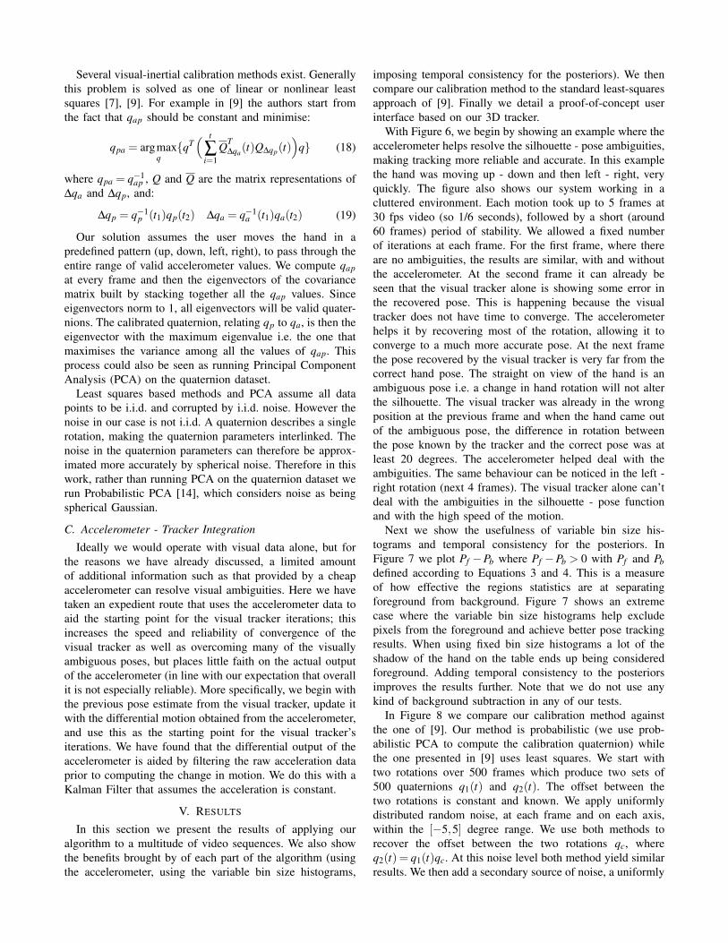
With Figure 6, we begin by showing an example where theaccelerometer helps resolve the silhouette - pose ambiguities,making tracking more reliable and accurate. In this examplethe hand was moving up - down and then left - right, veryquickly. The figure also shows our system working in acluttered environment. Each motion took up to 5 frames at30 fps video (so 1/6 seconds), followed by a short (around60 frames) period of stability. We allowed a fixed numberof iterations at each frame. For the first frame, where thereare no ambiguities, the results are similar, with and withoutthe accelerometer. At the second frame it can already beseen that the visual tracker alone is showing some error inthe recovered pose. This is happening because the visualtracker does not have time to converge. The accelerometerhelps it by recovering most of the rotation, allowing it toconverge to a much more accurate pose. At the next framethe pose recovered by the visual tracker is very far from thecorrect hand pose. The straight on view of the hand is anambiguous pose i.e. a change in hand rotation will not alterthe silhouette. The visual tracker was already in the wrongposition at the previous frame and when the hand came outof the ambiguous pose, the difference in rotation betweenthe pose known by the tracker and the correct pose was atleast 20 degrees. The accelerometer helped deal with theambiguities. The same behaviour can be noticed in the left -right rotation (next 4 frames). The visual tracker alone can’tdeal with the ambiguities in the silhouette - pose functionand with the high speed of the motion.

Next we show the usefulness of variable bin size his-tograms and temporal consistency for the posteriors. InFigure 7 we plot Pf −Pb where Pf −Pb > 0 with Pf and Pbdefined according to Equations 3 and 4. This is a measureof how effective the regions statistics are at separatingforeground from background. Figure 7 shows an extremecase where the variable bin size histograms help excludepixels from the foreground and achieve better pose trackingresults. When using fixed bin size histograms a lot of theshadow of the hand on the table ends up being consideredforeground. Adding temporal consistency to the posteriorsimproves the results further. Note that we do not use anykind of background subtraction in any of our tests.

In Figure 8 we compare our calibration method againstthe one of [9]. Our method is probabilistic (we use prob-abilistic PCA to compute the calibration quaternion) whilethe one presented in [9] uses least squares. We start withtwo rotations over 500 frames which produce two sets of500 quaternions q1(t) and q2(t). The offset between thetwo rotations is constant and known. We apply uniformlydistributed random noise, at each frame and on each axis,within the [−5,5] degree range. We use both methods torecover the offset between the two rotations qc, whereq2(t) = q1(t)qc. At this noise level both method yield similarresults. We then add a secondary source of noise, a uniformly

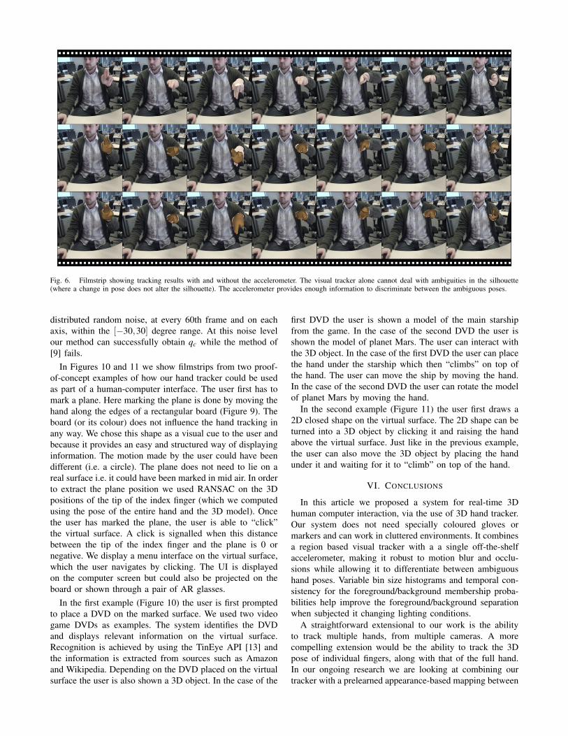
Fig. 6. Filmstrip showing tracking results with and without the accelerometer. The visual tracker alone cannot deal with ambiguities in the silhouette(where a change in pose does not alter the silhouette). The accelerometer provides enough information to discriminate between the ambiguous poses.

distributed random noise, at every 60th frame and on eachaxis, within the [−30,30] degree range. At this noise levelour method can successfully obtain qc while the method of[9] fails.

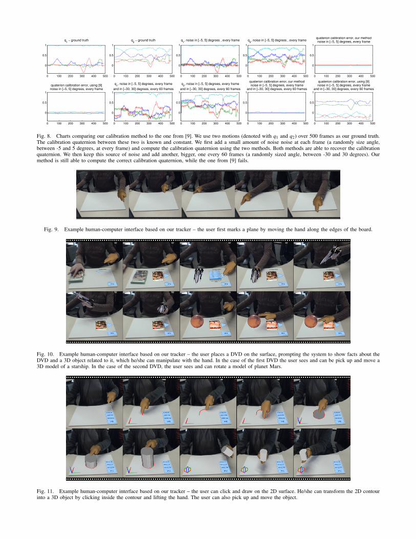
In Figures 10 and 11 we show filmstrips from two proof-of-concept examples of how our hand tracker could be usedas part of a human-computer interface. The user first has tomark a plane. Here marking the plane is done by moving thehand along the edges of a rectangular board (Figure 9). Theboard (or its colour) does not influence the hand tracking inany way. We chose this shape as a visual cue to the user andbecause it provides an easy and structured way of displayinginformation. The motion made by the user could have beendifferent (i.e. a circle). The plane does not need to lie on areal surface i.e. it could have been marked in mid air. In orderto extract the plane position we used RANSAC on the 3Dpositions of the tip of the index finger (which we computedusing the pose of the entire hand and the 3D model). Oncethe user has marked the plane, the user is able to “click”the virtual surface. A click is signalled when this distancebetween the tip of the index finger and the plane is 0 ornegative. We display a menu interface on the virtual surface,which the user navigates by clicking. The UI is displayedon the computer screen but could also be projected on theboard or shown through a pair of AR glasses.

In the first example (Figure 10) the user is first promptedto place a DVD on the marked surface. We used two videogame DVDs as examples. The system identifies the DVDand displays relevant information on the virtual surface.Recognition is achieved by using the TinEye API [13] andthe information is extracted from sources such as Amazonand Wikipedia. Depending on the DVD placed on the virtualsurface the user is also shown a 3D object. In the case of the

first DVD the user is shown a model of the main starshipfrom the game. In the case of the second DVD the user isshown the model of planet Mars. The user can interact withthe 3D object. In the case of the first DVD the user can placethe hand under the starship which then “climbs” on top ofthe hand. The user can move the ship by moving the hand.In the case of the second DVD the user can rotate the modelof planet Mars by moving the hand.

In the second example (Figure 11) the user first draws a2D closed shape on the virtual surface. The 2D shape can beturned into a 3D object by clicking it and raising the handabove the virtual surface. Just like in the previous example,the user can also move the 3D object by placing the handunder it and waiting for it to “climb” on top of the hand.

VI. CONCLUSIONS

In this article we proposed a system for real-time 3Dhuman computer interaction, via the use of 3D hand tracker.Our system does not need specially coloured gloves ormarkers and can work in cluttered environments. It combinesa region based visual tracker with a a single off-the-shelfaccelerometer, making it robust to motion blur and occlu-sions while allowing it to differentiate between ambiguoushand poses. Variable bin size histograms and temporal con-sistency for the foreground/background membership proba-bilities help improve the foreground/background separationwhen subjected it changing lighting conditions.

A straightforward extensional to our work is the abilityto track multiple hands, from multiple cameras. A morecompelling extension would be the ability to track the 3Dpose of individual fingers, along with that of the full hand.In our ongoing research we are looking at combining ourtracker with a prelearned appearance-based mapping between

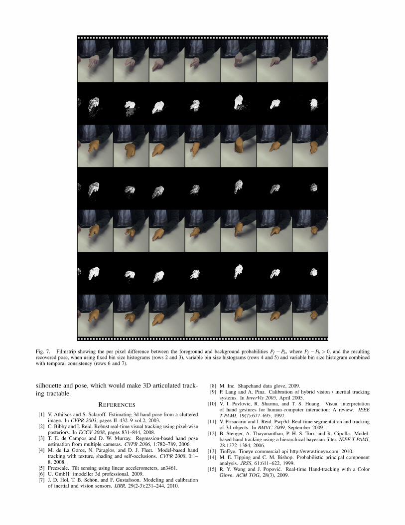
Fig. 7. Filmstrip showing the per pixel difference between the foreground and background probabilities Pf −Pb, where Pf −Pb > 0, and the resultingrecovered pose, when using fixed bin size histograms (rows 2 and 3), variable bin size histograms (rows 4 and 5) and variable bin size histogram combinedwith temporal consistency (rows 6 and 7).

silhouette and pose, which would make 3D articulated track-ing tractable.

REFERENCES

[1] V. Athitsos and S. Sclaroff. Estimating 3d hand pose from a clutteredimage. In CVPR 2003, pages II–432–9 vol.2, 2003.

[2] C. Bibby and I. Reid. Robust real-time visual tracking using pixel-wiseposteriors. In ECCV 2008, pages 831–844, 2008.

[3] T. E. de Campos and D. W. Murray. Regression-based hand poseestimation from multiple cameras. CVPR 2006, 1:782–789, 2006.

[4] M. de La Gorce, N. Paragios, and D. J. Fleet. Model-based handtracking with texture, shading and self-occlusions. CVPR 2008, 0:1–8, 2008.

[5] Freescale. Tilt sensing using linear accelerometers, an3461.[6] U. GmbH. imodeller 3d professional. 2009.[7] J. D. Hol, T. B. Schon, and F. Gustafsson. Modeling and calibration

of inertial and vision sensors. IJRR, 29(2-3):231–244, 2010.

[8] M. Inc. Shapehand data glove, 2009.[9] P. Lang and A. Pinz. Calibration of hybrid vision / inertial tracking

systems. In InverVis 2005, April 2005.[10] V. I. Pavlovic, R. Sharma, and T. S. Huang. Visual interpretation

of hand gestures for human-computer interaction: A review. IEEET-PAMI, 19(7):677–695, 1997.

[11] V. Prisacariu and I. Reid. Pwp3d: Real-time segmentation and trackingof 3d objects. In BMVC 2009, September 2009.

[12] B. Stenger, A. Thayananthan, P. H. S. Torr, and R. Cipolla. Model-based hand tracking using a hierarchical bayesian filter. IEEE T-PAMI,28:1372–1384, 2006.

[13] TinEye. Tineye commercial api http://www.tineye.com, 2010.[14] M. E. Tipping and C. M. Bishop. Probabilistic principal component

analysis. JRSS, 61:611–622, 1999.[15] R. Y. Wang and J. Popovic. Real-time Hand-tracking with a Color

Glove. ACM TOG, 28(3), 2009.

0 100 200 300 400 500

0

0.5

1

q1 − ground truth

0 100 200 300 400 500

0

0.5

1

q2 − ground truth

0 100 200 300 400 500

0

0.5

1

q1, noise in [−5, 5] degrees , every frame

0 100 200 300 400 500

0

0.5

1

q2, noise in [−5, 5] degrees , every frame

0 100 200 300 400 500

0

0.5

1

quaterion calibration error, our methodnoise in [−5, 5] degrees, every frame

0 100 200 300 400 500

0

0.5

1

quaterion calibration error, using [9]noise in [−5, 5] degrees, every frame

0 100 200 300 400 500

0

0.5

1

q1, noise in [−5, 5] degrees, every frame

and in [−30, 30] degrees, every 60 frames

0 100 200 300 400 500

0

0.5

1

q2, noise in [−5, 5] degrees, every frame

and in [−30, 30] degrees, every 60 frames

0 100 200 300 400 500

0

0.5

1

quaterion calibration error, our methodnoise in [−5, 5] degrees, every frame

and in [−30, 30] degrees, every 60 frames

0 100 200 300 400 500

0

0.5

1

quaterion calibration error, using [9]noise in [−5, 5] degrees, every frame

and in [−30, 30] degrees, every 60 frames

Fig. 8. Charts comparing our calibration method to the one from [9]. We use two motions (denoted with q1 and q2) over 500 frames as our ground truth.The calibration quaternion between these two is known and constant. We first add a small amount of noise noise at each frame (a randomly size angle,between -5 and 5 degrees, at every frame) and compute the calibration quaternion using the two methods. Both methods are able to recover the calibrationquaternion. We then keep this source of noise and add another, bigger, one every 60 frames (a randomly sized angle, between -30 and 30 degrees). Ourmethod is still able to compute the correct calibration quaternion, while the one from [9] fails.

Fig. 9. Example human-computer interface based on our tracker – the user first marks a plane by moving the hand along the edges of the board.

Fig. 10. Example human-computer interface based on our tracker – the user places a DVD on the surface, prompting the system to show facts about theDVD and a 3D object related to it, which he/she can manipulate with the hand. In the case of the first DVD the user sees and can be pick up and move a3D model of a starship. In the case of the second DVD, the user sees and can rotate a model of planet Mars.

Fig. 11. Example human-computer interface based on our tracker – the user can click and draw on the 2D surface. He/she can transform the 2D contourinto a 3D object by clicking inside the contour and lifting the hand. The user can also pick up and move the object.