riverine landscape dynamics and ecological risk assessment

Riverine landscape dynamics and ecologicalrisk assessment

ROB S. E. W. LEUVEN* and ISABELLE POUDEVIGNE†

*Department of Environmental Studies, Faculty of Science, Mathematics and Computing Science, University of Nijmegen,

Nijmegen, The Netherlands

†Laboratory of Ecology, UPRES-EA 1293, University of Rouen, 76281 Mont Saint Aignan, France

SUMMARY

1. The aim of ecological risk assessments is to evaluate the likelihood that ecosystems are

adversely affected by human-induced disturbance that brings the ecosystem into a new

dynamic equilibrium with a simpler structure and lower potential energy. The risk

probability depends on the threshold capacity of the system (resistance) and on the

capacity of the system to return to a state of equilibrium (resilience).

2. There are two complementary approaches to assessing ecological risks of riverine

landscape dynamics. The reductionist approach aims at identifying risk to the ecosystem

on the basis of accumulated data on simple stressor–effect relationships. The holistic

approach aims at taking the whole ecosystem performance into account, which implies

meso-scale analysis.

3. Landscape patterns and their dynamics represent the physical framework of processes

determining the ecosystem’s equilibrium. Assessing risks of landscape dynamics to

riverine ecosystems implies addressing complex interactions of system components (e.g.

population dynamics and biogeochemical cycles) occurring at multiple scales of space and

time.

4. One of the most important steps in ecological risk assessment is to establish clear

assessment endpoints (e.g. vital ecosystem and landscape attributes). Their formulation

must recognise that riverine ecosystems are dynamic, structurally complex and composed

of both deterministic and stochastic components.

5. Remote sensing (geo)statistics and geographical information systems are primary tools

for quantifying spatial and temporal components of riverine ecosystem and landscape

attributes.

6. The difficulty to experiment at the riverine landscape level means that ecological risk

management is heavily dependent on models. Current models are targeted towards

simulating ecological risk at levels ranging from single species to habitats, food webs and

meta-populations to ecosystems and entire riverine landscapes, with some including socio-

economic considerations.

Keywords: disturbance, habitat alteration, landscape dynamics, risk modelling, riverine ecosystems

Introduction

The term ‘riverine landscape’ implies a holistic geo-

morphic perspective of the extensive interconnected

series of habitats and environmental gradients that,

with their biotic communities, constitute fluvial sys-

tems (Ward, 1998). This type of landscape is highly

Correspondence: Dr Rob S. E. W. Leuven, Department

of Environmental Studies, Faculty of Science, Mathematics

and Computing Science, University of Nijmegen, PO Box 9010,

6500 GL Nijmegen, The Netherlands. E-mail: [email protected]

Freshwater Biology (2002) 47, 845–865

Ó 2002 Blackwell Science Ltd 845

dynamic, showing a constantly changing mosaic of

habitats (Stanford et al., 1996; Ward et al., 2002).

Hydrological processes (e.g. flood pulse) and geomor-

phological processes (e.g. sedimentation and erosion)

are key processes of natural river systems. The

environmental gradients and natural disturbance

regimes that characterise these open systems make

them complex and diverse systems that are very

sensitive to human activities (Bornette et al., 1998;

Ward, 1998). The fertile and flat soils of the river

floodplains tend to be highly modified by agricultural

land use, urbanisation and industrialisation (Smits,

Nienhuis & Leuven, 2000), and the hydrology and

morphology of the riverine systems are altered by flow

regulation, channelisation and bank stabilisation

(Petts, Moller & Roux, 1989). Estuaries are particularly

important as they are the endpoints of catchment-wide

fluvio-ecological processes, as well as socio-economic

activities, often with high human population densities

(Vitousek, 1994; Nienhuis, Leuven & Ragas, 1998;

Noss, 2000). The resulting loss of physical relationship

among the systems’ abiotic components leads to loss of

interaction potential among the other system compo-

nents such as population dynamics of wildlife and

biogeochemical cycles (Ward, 1998; Tockner et al.,

1999; Ward, Tockner & Schiemer, 1999). Habitat

alteration (including habitat loss, degradation and

fragmentation) has been the focus of many studies

concerned with ecological integrity, sustainability and

ecosystem health (Rapport, 1992; Hobbs, 1993; Baker,

1995; Hanski et al., 1995). As one of the main driving

forces behind habitat alteration, landscape dynamics is

considered as a major issue in ecological risk assess-

ment (Turner, 1994; Noss, 2000).

Risk is a combination of two factors: (1) the

probability that an adverse event will occur; and (2)

the consequences of the adverse event (Presidential/

Congressional Commission on Risk Assessment and

Risk Management, 1997). Ecological risk encompasses

impacts on the structure and function of ecosystems,

and arises from exposure and hazard. Hazard

depends upon whether a particular substance or

situation has the potential to cause harmful effects.

Ecological risk assessment has been defined as a

process that evaluates the likelihood that adverse

ecological effects may occur or are occurring as a

result of exposure to one or more stressors (US-EPA,

1992; Suter, 1993). This process includes problem

formulation as well as characterisation of exposure,

ecological effects and risks (Presidential/Congres-

sional Commission on Risk Assessment and Risk

Management, 1997).

To make an effective risk management, river man-

agers and other stakeholders need to know what

potential harm riverine landscape dynamics pose, and

how great is the likelihood that riverine ecosystems

will be harmed. In spite of the fact that it is a rather

recent domain in environmental sciences, ecological

risk assessment over the past 20 years has a large

literature, but with little at the riverine landscape

level. Although not comprehensive, the present

review provides an introduction to ecological risk

assessment related to riverine landscape dynamics.

It focuses on floodplains and riparian zones rather

than river habitat, because several other reviews

already deal with the more traditional aquatic

approach (e.g. Cook, Suter & Sain, 1999; Culp, Lowell &

Cash, 2000). It aims at answering the following

questions: (1) What are the different approaches to

assessing ecological risks? (2) How can landscape

ecological concepts contribute to risk assessment? (3)

How are pattern and process in changing landscapes

related? (4) When does ecosystem disturbance imply

ecological risk? (5) What are the endpoints for

ecological risk assessments, and which of the entities

and attributes of the riverine ecosystem do society

value? (6) What are the tools (with special attention to

data acquisition and processing) to assess ecological

risks in changing riverine landscapes? Finally (7), the

recent advances in ecological risk assessment of

riverine landscape dynamics and recommendations

for future research are discussed.

Ecological risk approaches

In general, there are two complementary approaches

to assessing ecological risks: the reductionist and

holistic approach (cf. Weber & Schmid 1995).

The reductionist approach

The reductionist approach aims at identifying risk to

the ecosystem on the basis of accumulated data on

simple stressor–effect relationships (e.g. the effect of

cadmium pollution on a local fish population). It

attempts to provide a series of threshold indices

which determine the probability that, at a certain

spatial and temporal scale, a component of the

846 R.S.E.W. Leuven and I. Poudevigne

Ó 2002 Blackwell Science Ltd, Freshwater Biology, 47, 845–865

ecosystem will be altered. These threshold indices can

then be combined into a conceptual model that

estimates the ecosystem response.

Evaluating risk to an ecosystem with a reductionist

approach involves considerable work to provide

information for each ecological, spatial and temporal

scale, as well as for all the responses of the ecosystem

(i.e. changes in structural and functional attributes) to

the stressor or set of multiple stressors (Leuven et al.,

1998). This can be achieved through diachronic

experimentation, which has the advantage of being

replicable and providing causation, or with syn-

chronic approaches (e.g. gradient analysis), which

have the advantage of being closer to reality but

which requires that the full range of stressor levels be

available and that the compared ecosystems be

effectively comparable. Recently, gradient analysis

has gained increasing recognition (Rey Benayas &

Scheiner, 1993; Hoagland & Collins, 1997; Tockner

et al., 1999). However, multiple stressors have mul-

tiple and sometimes opposing effects on aquatic biota,

making interpretation at a regional scale difficult.

Lowell, Culp & Dube (2000) have addressed this

problem by a weight-of-evidence approach that com-

bines analysis of field data (gradient analysis and

other field surveys to determine patterns) with

experimental hypothesis testing (integrating meso-

cosm studies with field and laboratory experiments to

determine mechanisms). This approach allows one,

for example, to make predictions of effects of toxic

substances, nutrient loading and winter freeze-up on

benthic biota and to provide appropriate river man-

agement recommendations.

The holistic approach

The holistic approach aims at taking the whole

ecosystem performance into account, which implies

meso-scale analysis (Lemly, 1997; Lawton, 1999). The

essential aspect of holism as a scientific assumption is

that it provides the basis for studying ecosystems

without knowing all the details of their internal

structure and functions (Zonneveld, 1990). It attempts

to provide a probability that the process of ecosystem

development (ecological succession), as a whole, may

change trajectory (e.g. see section risks of ecosystem

disturbance and Figs 1–3).

Holism permits the simplification of scientific

activity by reducing analytic observations so as better

to understand very complex structures and processes

(Zonneveld, 1990). It removes the necessity of first

defining all the elements and their mutual relation-

ships before defining the whole. At the same time it

warns against attempting to study wholes by analy-

sing them in separate pieces without connecting them

with each other. The holistic approach is based on the

use of indicators of ecosystem health, just like

temperature is an indicator of human health (Rapport,

1992; Cairns, 1999; Costanza & Mageau, 1999).

Recently, the health metaphor has also been applied

to the assessment of river and landscape conditions

(Sparks, 1995; Ferguson, 1996; Boulton, 1999; Fair-

weather, 1999; Norris & Thoms, 1999).

Contribution of landscape ecological concepts

to risk assessment

Many fields of science have contributed to the

development and enrichment of concepts for ecolog-

ical risk assessment, e.g. ecotoxicology, conservation

biology and restoration ecology. An important contri-

bution is that of landscape ecology (Johnson & Gage,

1997). Landscape ecology addresses ecosystem integ-

rity by considering the spatial and temporal attributes

of landscapes and considering that patterns and

processes are hierarchically linked (Wiens et al.,

1993; Pickett & Cadenasso, 1995; Muller, 1992; Wiens,

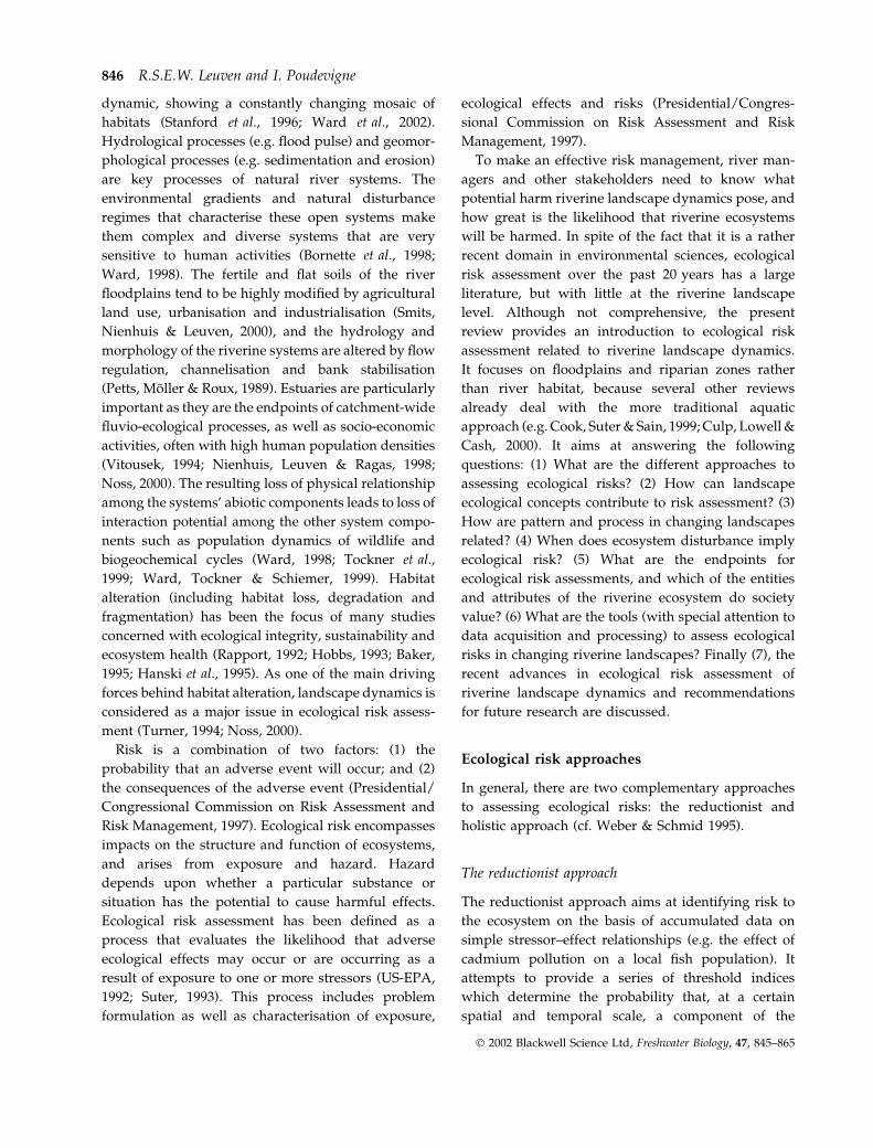
Fig. 1 Stability states of ecosystems in terms of potential energy

or complexity (adapted from Godron & Forman, 1983). Point B is

the most stable. Points C, D, and E are metastable. Points A, L,

M, N and Z are unstable. The transitions from B to C and to E are

difficult, but increase the degree of metastability; such a

progression corresponds to a series of successional stages that

begins with the most stable state, moves rapidly to the least

stable state, and thereafter gradually increase its metastability.

Transitions from E to D, to C and to B are less difficult; they

correspond to a degradation of the ecological system.

Riverine landscape dynamics 847


2002). The attributes of landscape which may be

relevant to approach ecological problems fall into at

least three categories: patch quantity and quality (e.g.

physico-chemical characteristics), patch structure

(e.g. sizes and biomass) and patch organisation (e.g.

relationships or specificity). Landscape changes can

affect one or several landscape attributes, which in

turn may affect ecological attributes such as the

hydrologic cycle, nutrient cycling or biodiversity.

The following paragraphs focus on the appropriate

scale and hierarchical framework to analyse ecological

risk of landscape change.

The interface between human activitiesand ecosystem: scale of analysis

Many early ecological risk assessments were per-

formed at very small spatial scales (e.g. estimations of

a site-specific risk for a single species) or at a very

large scale (e.g. global risk assessments of greenhouse

gases), but rarely at the landscape (or mesoscale)

level. Today, in many riverine landscapes, and espe-

cially along regulated rivers, disturbances associated

with human activities have replaced or accentuated

natural disturbances (Baker, 1995). Indeed the com-

monest disturbances that alter ecosystem integrity are

now anthropogenic. Stream regulation for example

reduces flow amplitude, induces temperature chan-

ges, alters material transport and major biophysical

patterns (Stanford et al., 1996; Ward, 1998), while

agricultural and industrial activities are an important

source of disturbance to nutrient cycling and contam-

inant introduction (Nebbache et al., 2001; Vitousek

et al., 1997). As most of these activities (including

management) address the landscape level, landscapes

have increasingly become the relevant level of obser-

vation for analysing risks to ecosystem integrity.

A hierarchical framework to analyse riskat each organisation level

Rather than using just a mesoscale approach, land-

scape ecology increasingly takes on a nested hierar-

chical approach (Urban, O’Neill & Shugart, 1987).

Hierarchy theory postulates that: (1) spatial and

temporal scales are closely linked, i.e. any process

occurring on a broad spatial scale occur on a long

temporal scale while short-term processes tend to be

more localised; (2) processes with different ‘rates of

behaviour’ are likely to be independent; and (3)

higher organisation levels constrain processes of the

lower levels, while lower levels of organisation

impose limiting conditions. The aim of such a nested

hierarchical approach is to break down complex

ecosystem processes into simpler levels of ecological

organisation which can more easily be reassembled in

a bottom-up process (Wu, 1999; Levin, 1999). Each

process determining an ecosystem’s integrity involves

several spatio-temporal levels of organisation.

The organisation of a system depends on the nature

and the intensity of the relationships between the

different elements defining that system. From a

methodological point of view, this offers the possibil-

ity to measure the organisation of a landscape (in

terms of mutual relationships between flooding,

agricultural, habitat and landscape patterns), or the

organisation of a species assemblage (in terms of

interspecies relationships such as competition or niche

partitioning). The concept of organisation also has

relevance for the stability of ecosystems (Kolasa &

Pickett, 1989). An organised system is supposed to be

a stable or rather metastable one (sensu Levin, 1976).

In that sense, measurements of attributes that refer to

stability of ecosystems may also provide insight into

the risk of ecosystem change.

Providing a spatial and temporal framework

to analyse risk

Whether focusing on the ecosystem as a whole or on

its components, many ecological risk assessments

have been performed on evaluations of the mean

(e.g. mean effect of cadmium ingestion on fish

reproductive rates). Others are focused on general

risk levels for a total floodplain (e.g. Noppert et al.,

1993; Hendriks et al., 1995), but do not account for

spatial and temporal aspects of exposure to stressors.

However, as stated before, riverine landscapes are

very dynamic, open systems and ecological processes

in them vary in space and time. The variability of

diffuse soil contamination in river floodplains, for

example, is very high and low pollutant concentra-

tions can be found only a short distance from sites

with relatively high contamination (Middelkoop

& Asselman, 1998; Schouten et al., 2000; Kooistra

et al., 2002). As a result of the spatial and temporal

variability of soil contamination, members of a group

of mobile terrestrial organisms are unlikely to be



exposed to the same level of contamination (Clifford

et al., 1995; Kooistra et al., 2001b). Thus, the relevance

of risk assessment is very dependent on the spatial

and temporal attributes of the stressor and the

responding ecosystem component (Forman & Collin-

ge, 1997; Risser, 1992). Model results have confirmed

the need to incorporate such information (Marinussen

& Van der Zee, 1996; McCarthy & Lindenmayer, 2000;

Kooistra et al., 2001b).

Relating pattern to process in a changing

landscape

The quality, structure and organisation of riverine

landscapes are the result of interactions between

human or natural disturbances and the ecosystem

(Ward, 1998). As such, assessing landscape attributes

and linking them to attributes of the ecosystem

provides one way to analyse risk to ecosystem

integrity. A very wide array of landscape measures

exists (for reviews, see Godron & Forman, 1983;

Cullinan & Thomas, 1992; McGarigal & Marks, 1995),

but rather few studies have been successful in relating

pattern to process (Levin, 1992; Alard & Poudevigne,

2002).

Landscapes, and more so riverine landscapes, are

not stable systems in equilibrium, but are dynamic.

Thus, most studies relating pattern to process have

focused on the range of variation in pattern with

regard to the range of variation in process. A major

part of these pattern-process studies have related a

pattern of species distribution (species assemblage

composition or organisation) to changes in landscape

quality or structure (Huston, 1994; Miller, Brooks &

Croonquist, 1997; Stohlgren et al., 1997). Several

authors, including Manel, Buckton & Ormerod

(2000) and Pearson (1993), have successfully related

bird assemblages to landscapes attributes. Others, like

Vos & Chardon (1998), showed a significant negative

correlation between herpetofauna species richness

and increasing road density. Both Hanski et al.

(1995) and Collinge & Forman (1998) have related

changes in land use with decreases in insect popula-

tions. The relation between fragmentation and species

composition has received much attention by meta-

population ecologists (With, Gardner & Turner, 1997;

Lenders et al., 1998b; Chardon, Foppen & Geilen,

2000). Fragmentation of riverine landscape has also

been related to alteration of ecosystem processes such

as the hydrologic cycle, nutrient cycle, radiation

balance and wind regime (Clark, 1991; Hobbs, 1993;

Hornung & Reynolds, 1995).

Risks of ecosystem disturbance

Riverine ecosystems have been described as changing

ecosystems far from equilibrium, alternating between

periods of relative stasis and dramatic change (Levin,

1999; Ward et al., 1999; Poudevigne et al., 2002b). Such

ecosystems may go through regular cycles of self-

organisation and collapse (Holling, 1987, 1995). Alter-

native states depend on the nature and intensity of the

interactions among the systems components (Carpen-

ter, Brock & Hansen, 1999). Ecosystems may exhibit

strong homeorhesis, that is, wide variability and more

than one stable condition, although they still have

limits of tolerance that mark the transition between

one state and another. As Cairns (2000) puts it, ‘the

best state is a matter for conjecture, although humans

clearly would prefer that ecosystems maintain a state

favourable to human life’.

Fig. 1 illustrates various (meta)stable states of eco-

systems in terms of potential energy or complexity,

based on the classical characteristics of stability in

mechanics (Godron & Forman, 1983). The ‘balls’ lying

in a ‘bowl’ symbolically represents states of stability

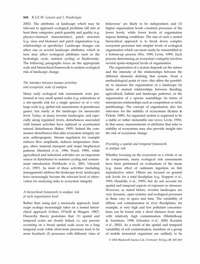
Fig. 2 Visualisation of various trajectories of ecological succes-

sion (in terms of potential energy) in a stressful environment

(adapted from Balent et al., 1999). 1: resistance of the ecosystem

despite the presence of disturbances (essentially unchanged

trajectory); 2, 3 and 4: resilience of the ecosystem after a

temporary low, moderate and high disturbance, respectively

(returning to reference trajectory); 5: ecosystem changes traject-

ory if the disturbance crosses a vital threshold value.



(Grimm, 1996). Living organisms often start from

highly stable states (e.g. bare floodplain soil or

bedrock), represented as state B in Fig. 1. Organisms

build locally metastable structures which are more

complex and have less entropy, represented by points

C, D and E. Hence, natural successional stages from

bare soil to floodplain forest proceed towards states of

increasing metastability. The natural riverine land-

scape must be analogous to the metastable point E. The

system is at risk of collapsing when a disturbance

pushes the ball out of its bowl into another state

(Godron & Forman, 1983; Kolasa & Pickett, 1989; Wu,

1999). Such a scenario occurs when one or several vital

thresholds have been crossed in the disturbance

process. These thresholds may concern one or several

levels of organisation. When more complex ecosys-

tems (higher levels of organisation) are concerned,

hierarchy theory would imply that the risk of system

collapse is higher than if less complex systems are

concerned (Pickett et al., 1989). The disturbed ecosystem

will eventually adjust to another ‘metastable condi-

tion’ where the ecosystem is in ‘equilibrium’ with its

external constrains (Godron & Forman, 1983; Kolasa &

Pickett, 1989). It is generally thought that the new

metastable position corresponds to a lower degree of

organisation or (potential) energy (Levin, 1992), at

least in the first stages of the disturbance before the

system has had time to accumulate energy again

(Holling, 1995). The more thresholds have been

passed, the more time and energy will be required

to restore an ecosystem (Aronson et al., 1993). An alter-

native model to simplify the underlying principles of

metastability in dynamic ecosystems is Holling’s four-

box model, which visualises the evolution of a

particular system in terms of so-called conservation,

release, exploitation and re-organisation states

(Holling, 1987; Costanza et al., 1993; Costanza, 1995).

The response of an ecosystem to disturbance varies

not only with the intensity and spatio-temporal

amplitude of the disturbance (Van der Maarel, 1993),

but also with the stability (or relative stability)

properties of the ecosystem (Holling, 1973; Wissel,

1984; Nienhuis & Leuven, 1997). Various measures

have been proposed for the different aspects of this

response, i.e. resistance, resilience and elasticity

(Grimm, 1996; Aarts & Nienhuis, 1999). Resistance is

the ability of ecosystems to show little response to

disturbance. Resilience defines the capacity of the

system to ‘return’ to its original successional trajectory

after a temporal disturbance. How long this return

will take is often denoted as elasticity. When the

disturbance causes the system to cross vital thresh-

olds, the system does not persist in its former

trajectory. According to this conceptual framework,

the relation between disturbance and risk could then

be hypothesised as follows (Fig. 2):

– If the disturbance is of low intensity and of small

spatial scale, the disturbance can cause changes in

patch dynamics (local heterogeneity within the

habitats), which would probably leave most eco-

logical processes unaffected overall (Veblen, 1992).

Patch disturbance can be seen as the creation of

gaps. In riverine landscapes, for example, trampling

from livestock or water flows that uproot trees

create gaps of small sizes (from cm2 to m2).

However, the ecosystem as a whole maintains its

trajectory and can be regarded as resistant (Fig. 2:

disturbance 1). Disturbance in this case is not likely

to imply risk to the riparian ecosystem.

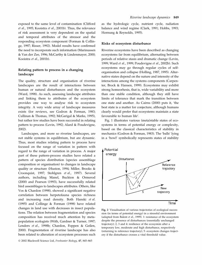
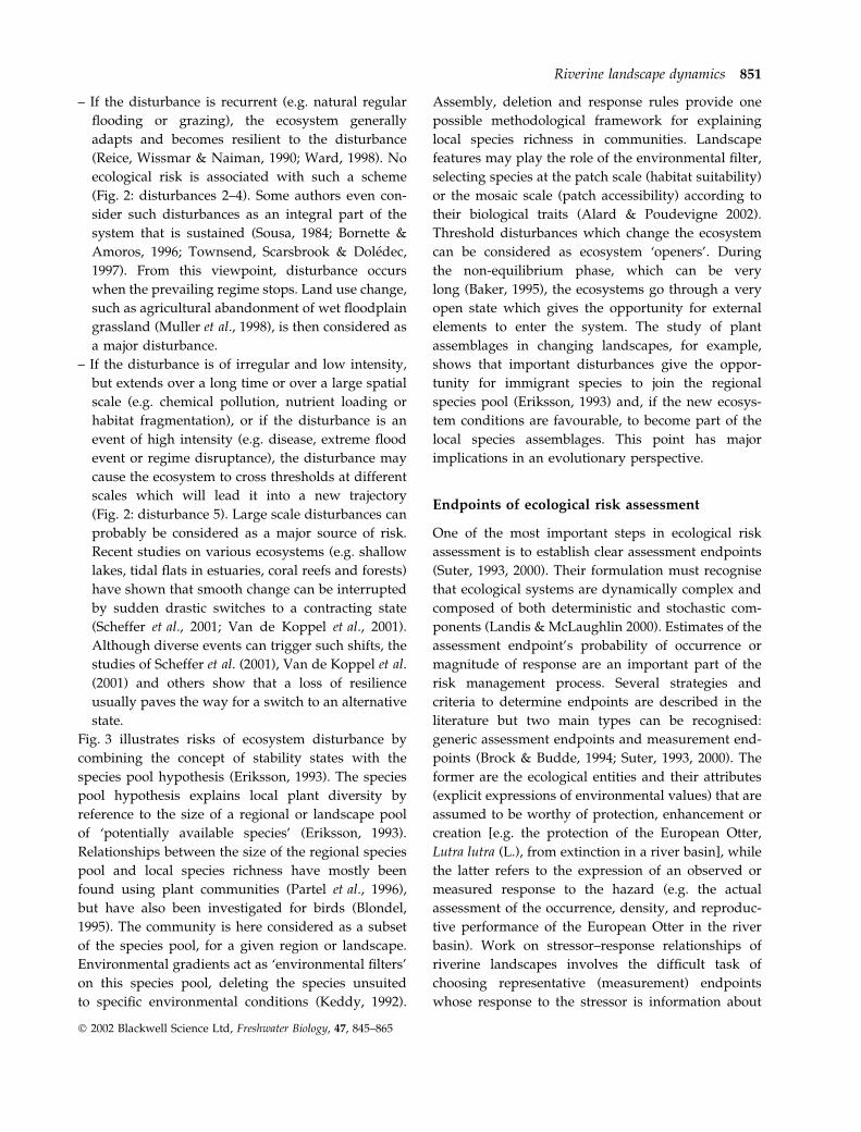
Fig. 3 Visualisation of the risks of ecosystem disturbance by

combining the concept of stability states with the species pool

hypothesis. For explanation of stability states during ecosystem

succession or degradation see Fig. 1. The funnels depict envi-

ronmental filters for species pools at various levels of organi-

sation (e.g., from regional to local environmental filters). A

threshold disturbance will force the ecosystem into a new

metastable situation and opens the species assemblages for

immigrants. The species pool arrows indicate the way in which,

at the various levels of organisation, the environmental factors

filter the non-adapted species of the regional species pool. LF:

local filters; LSA: local species assemblages; RF: regional filters.



– If the disturbance is recurrent (e.g. natural regular

flooding or grazing), the ecosystem generally

adapts and becomes resilient to the disturbance

(Reice, Wissmar & Naiman, 1990; Ward, 1998). No

ecological risk is associated with such a scheme

(Fig. 2: disturbances 2–4). Some authors even con-

sider such disturbances as an integral part of the

system that is sustained (Sousa, 1984; Bornette &

Amoros, 1996; Townsend, Scarsbrook & Doledec,

1997). From this viewpoint, disturbance occurs

when the prevailing regime stops. Land use change,

such as agricultural abandonment of wet floodplain

grassland (Muller et al., 1998), is then considered as

a major disturbance.

– If the disturbance is of irregular and low intensity,

but extends over a long time or over a large spatial

scale (e.g. chemical pollution, nutrient loading or

habitat fragmentation), or if the disturbance is an

event of high intensity (e.g. disease, extreme flood

event or regime disruptance), the disturbance may

cause the ecosystem to cross thresholds at different

scales which will lead it into a new trajectory

(Fig. 2: disturbance 5). Large scale disturbances can

probably be considered as a major source of risk.

Recent studies on various ecosystems (e.g. shallow

lakes, tidal flats in estuaries, coral reefs and forests)

have shown that smooth change can be interrupted

by sudden drastic switches to a contracting state

(Scheffer et al., 2001; Van de Koppel et al., 2001).

Although diverse events can trigger such shifts, the

studies of Scheffer et al. (2001), Van de Koppel et al.

(2001) and others show that a loss of resilience

usually paves the way for a switch to an alternative

state.

Fig. 3 illustrates risks of ecosystem disturbance by

combining the concept of stability states with the

species pool hypothesis (Eriksson, 1993). The species

pool hypothesis explains local plant diversity by

reference to the size of a regional or landscape pool

of ‘potentially available species’ (Eriksson, 1993).

Relationships between the size of the regional species

pool and local species richness have mostly been

found using plant communities (Partel et al., 1996),

but have also been investigated for birds (Blondel,

1995). The community is here considered as a subset

of the species pool, for a given region or landscape.

Environmental gradients act as ‘environmental filters’

on this species pool, deleting the species unsuited

to specific environmental conditions (Keddy, 1992).

Assembly, deletion and response rules provide one

possible methodological framework for explaining

local species richness in communities. Landscape

features may play the role of the environmental filter,

selecting species at the patch scale (habitat suitability)

or the mosaic scale (patch accessibility) according to

their biological traits (Alard & Poudevigne 2002).

Threshold disturbances which change the ecosystem

can be considered as ecosystem ‘openers’. During

the non-equilibrium phase, which can be very

long (Baker, 1995), the ecosystems go through a very

open state which gives the opportunity for external

elements to enter the system. The study of plant

assemblages in changing landscapes, for example,

shows that important disturbances give the oppor-

tunity for immigrant species to join the regional

species pool (Eriksson, 1993) and, if the new ecosys-

tem conditions are favourable, to become part of the

local species assemblages. This point has major

implications in an evolutionary perspective.

Endpoints of ecological risk assessment

One of the most important steps in ecological risk

assessment is to establish clear assessment endpoints

(Suter, 1993, 2000). Their formulation must recognise

that ecological systems are dynamically complex and

composed of both deterministic and stochastic com-

ponents (Landis & McLaughlin 2000). Estimates of the

assessment endpoint’s probability of occurrence or

magnitude of response are an important part of the

risk management process. Several strategies and

criteria to determine endpoints are described in the

literature but two main types can be recognised:

generic assessment endpoints and measurement end-

points (Brock & Budde, 1994; Suter, 1993, 2000). The

former are the ecological entities and their attributes

(explicit expressions of environmental values) that are

assumed to be worthy of protection, enhancement or

creation [e.g. the protection of the European Otter,

Lutra lutra (L.), from extinction in a river basin], while

the latter refers to the expression of an observed or

measured response to the hazard (e.g. the actual

assessment of the occurrence, density, and reproduc-

tive performance of the European Otter in the river

basin). Work on stressor–response relationships of

riverine landscapes involves the difficult task of

choosing representative (measurement) endpoints

whose response to the stressor is information about



the ecosystem as a whole (holistic approach), or about

specific components of the ecosystem (reductionist

approach).

A large variety of ecosystem goods (such as food)

and services (such as waste assimilation) associated

with riverine landscapes are recognised as worthy of

protection (De Groot, 1992; Pratt & Cairns, 1993;

Richardson, 1994 Costanza et al., 1997; Daily, 1997;

Lemly, 1997; Moss, 2000; Vorenhout, Van Straalen &

Eijsackers, 2000). For example, hydrologic flux and

storage capacity of these landscapes are valued for

their flood control or water supply capacities. Bio-

logical productivity is valued for timber production,

reed bed production, grazing and food production.

More recently, the value of habitat diversity and

biodiversity have been increasingly recognised (either

for recreational purposes or biological conservation).

Biogeochemical cycling and storage capacities are

valued for preserving water quality, nutrient removal

or sediment pollution control. These ecosystem func-

tions can be used to derive endpoints for risk

assessments.

Ecosystem integrity requires the maintenance of

both physico-chemical and biological integrity (Karr

& Dudley, 1981). This means that ecological risk

assessments should focus on risks to the processes

which maintain ecosystem integrity (Noss, 1990).

Assessing this integrity is most often addressed with

a set of indicators that can provide a suite of multiple

lines of information on the structure and functioning

of the ecosystem. In such a case, ecological risk

assessments involves estimating for reference areas

changes in indicator values away from a defined

condition. Selecting the reference conditions is a

complex issue which involves choosing among the

most critical processes, based upon the valuation of

socio-economical criteria or ecological criteria or both

(Aronson et al., 1993; Tapsell, 1995; Lenders et al.,

1998a; Nienhuis & Leuven 2001). Reference conditions

can be determined on the basis of historical data

(palaeo-references), data derived from actual situa-

tions elsewhere (actuoreferences), knowledge about

system structure and functioning in general (system

theoretical references), or a combination of these

sources (Petts & Amoros, 1996; Jungwirth et al.,

2002). Restoration ecology provides us with many

indices of ecosystem integrity based on the emergent

properties of the system. Kelly & Harwell (1990)

provide an overview for aquatic ecosystems (partic-

ularly streams and rivers) of attributes indicating

ecosystem recovery. Numerous measurement end-

points for aquatic communities and biota can also be

found in the literature on field tests for hazard

assessment of chemicals (Brock & Budde, 1994; Suter,

2000). Many of them are the backbone of ecological

risk assessment in rivers. Aronson et al. (1993) des-

cribe what they call ‘vital ecosystem attributes’

(Table 1) that together, when studied over sufficient

periods of time, will permit appraisal and comparison

of system-wide responses to a given disturbance. On

the basis that landscapes are the physical framework

for ecological processes, Aronson & Le Floc’h (1996)

have complemented their list of ecological attributes

with a list of ‘vital landscape attributes’ (Table 2).

These can provide quantitative indicators for levels of

landscape degradation and can play a critical role in

directing landscape dynamics.

Other indices are based on the concept of organisa-

tion (see section on landscape ecological concepts) and

refer to the stability or complexity of the system. Most

indices used for analysing landscape organisation are

based on information theory (De Pablo et al., 1988;

Phipps, 1981) and geostatistics (Burrough, 1981). The

degree of redundancy (mutual information) between

an attribute of the landscape (e.g. land use) and a set of

explanatory variables (e.g. type of soil, distance to farm

Structural attributes Functional attributes

1. Species richness of perennials 1. Biomass productivity

2. Species richness of annuals 2. Soil organic matter

3. Total plant cover 3. Maximum available soil water reserves

4. Above-ground phytomass 4. Coefficient of rainfall efficiency

5. Beta diversity 5. Rain use efficiency

6. Life-form spectrum 6. Length of water availability period

7. Keystone species 7. Nitrogen use efficiency

8. Microbial biomass 8. Microsymbiotic effectiveness

9. Soil biota diversity 9. Cycling indices

Table 1 Vital ecosystem attributes for

evaluating stages of degradation (Aronson

et al., 1993)



or slope) provides an indication of how the system is

organised. Calculations of such a measure for the

landscape of the lower Seine valley between 1965 and

1999 show how this landscape shifts from a traditional

agricultural organisation (‘one soil-one use’) to a less

coherent organisation (‘any soil-any use’) (Poudevigne

et al., 1997). The few available indices focusing on

ecological organisation measure how ecological

response varies along landscape gradients (Balent &

Courtiade, 1992; Thioulouse & Chessel, 1992; Alard &

Poudevigne, 2002). An example is reciprocal scaling of

species along environmental gradients obtained from

ordination analysis. This procedure provides a meas-

ure of the ecological coherence (or organisation) of the

species assemblages along the environmental gradient.

Less coherent assemblages are commonly associated

with recent shifts in the set of factors which organise

them. It can be hypothesised that these assemblages

are more vulnerable to disturbance (less stable, open

systems described in the previous section). Several

studies in the Seine valley have focused largely on the

application of these indices of ecosystem change; the

predictive value of these indices was tested both on

fauna (ecological organisation of birds in a wetland of

the lower valley) (Poudevigne et al., 2002a) and on

higher plants (Alard & Poudevigne, 2000, 2002;

Poudevigne et al., 2002b).

When species are the focus of risk assessments,

indicators generally involve several taxa (e.g.

mammals, birds, amphibians, macro-invertebrates

and algae). The choice of such test species is critical

as the response to the stressors is highly diverse

(Alard et al., 1998; Admiraal et al., 2000; Stahl et al.,

2000). Indicator species have often been selected for

their vulnerability to changes in the vital attributes of

landscapes. Lambeck (1997) identified area-limited

species, dispersal-limited species, resource-limited

species, and process-limited species as potentially

vulnerable groups. Ormerod & Watkinson (2000)

remark that birds are often chosen as indicators as

‘their patterns of behaviour, distribution, seasonal

phenology and demography track closely onto spatial

and temporal scales’ of human activities (namely

agriculture). A useful measure of toxic stress on

species assemblages is the potentially affected frac-

tion; this is the fraction of species exposed to concen-

trations above the no observed effect level, and taking

account of differences between laboratory and field

tests of bioavailability (Klepper et al., 1999).

Tools to assess ecological risks

Geographic information systems

Geographic information systems (GIS) have now been

in use for several decades and are having a pervasive

impact on the way ecological risk assessment is

carried out (Leuven, Poudevigne & Teeuw, 2002).

Burrough & McDonnell, 1998) define a GIS as ‘a

powerful set of tools for collecting, storing, retrieving

at will, transformation and displaying spatial data

from the real world for a particular set of purposes’.

The input of high-quality data is essential for a good

GIS performance. Data input covers all aspects of

capturing spatial data from existing maps and field

surveys. Over the last few decades, many new ways to

collect and process spatial data have appeared, and

especially remotely sensed data (see next section;

Mertes, 2002). With reliable data, there is still a risk

that inappropriate data processing will produce un-

reliable results, although the GIS-generated output

might look convincing.

GIS can be utilised as the primary tool for the

quantification of spatial heterogeneity and temporal

components of ecosystems and landscape attributes

(Leuven, Poudevigne & Teeuw, 2002). Gordon &

Majumder (2000) applied GIS for integrating and

summarising data on empirical stressor–effect

Table 2 Vital landscape attributes indicating landscape degra-

dation (Aronson & Le Floc’h, 1996)

1. Type, number and range of landforms

2. Number of ecosystems present

3. Type, number and range of land units

4. Diversity, length, and intensity of former human uses

5. Diversity of present human uses

6. Number and proportion of land use types

7. Number and variety of ecotones

8. Number and types of corridors

9. Diversity of selected critical groups of organisms

(or functional groups)

10. Range and modalities of organisms regularly crossing

ecotones

11. Cycling indices of flows and exchanges of water, nutrients

and energy within and among ecosystems

12. Pattern and flux of water and nutrients

13. Levels of anthropogenic transformation of a landscape

14. Spread of disturbances

15. Number and importance of biological invasions

16. Nature and intensity of the different sources of degradation



relationships for prospective risk analysis. The effects

of land use and instream physical and chemical

factors on a biological indicator, the index of biotic

integrity, have been studied using nested catchments

and geographic units. Dyer et al. (2000) utilised GIS to

investigate over large geographic areas bottom-up

and top-down approaches for assessing effects of

multiple stressors (e.g. instream habitat, drainage

area, cumulative effluent) on the index of biotic

integrity (i.e. subbasin and basin level). Recently,

Kooistra et al. (2001b, 2002) presented a procedure

that incorporates spatial and temporal variability of

floodplain pollution into ecological risk assessment by

linking a GIS with models that estimate exposure of a

typical floodplain food web (Fig. 4). The procedure

uses readily available site-specific data and is applic-

able to a wide range of locations and floodplain

management scenarios. As first step, an explicit

statement of assessment endpoints and associated

functions or qualities that have to be maintained or

protected is formulated. Step 1 results in hypotheses

and research questions. Several types of data are

required for ecological risk assessment: autoecological

data about the species present when the desired

endpoint is reached (e.g. diet and food intake rate),

ecotoxicological information (e.g. bioaccumulation

factors and toxicity reference values), and information

describing the spatial and temporal variability of

environmental factors in the floodplain (e.g. topogra-

phy, geology, soil types, groundwater tables, veget-

ation, point data on soil pollution). Step 2 focuses on

data collection, selection and processing. Spatial

variability of pollutants is quantified by overlaying

appropriate topographic and soil maps with known

habitat requirements of focal species, resulting in the

definition of homogeneous habitat patches and pol-

lution concentration maps (step 3). In step 4, the GIS is

used to include spatial and temporal components of

the exposed organisms in the food web. Risk estimates

from a probabilistic exposure model (step 5) are used

Fig. 4 A procedure for the incorporation

of spatial and temporal variability of soil

pollution into the ecological risk analysis

of river floodplains, by linking a geo-

graphical information system (GIS) with a

model that estimates exposure of a food

web to a pollutant (adapted from Kooistra

et al., 2001b).



to construct site-specific risk data and maps for the

floodplain (step 6) and to evaluate ecological risks

(step 7). Fig. 5 summarises the features of an exposure

model that has been used and gives an example of the

model output (i.e. a site-specific ecotoxicological risk

estimation for the little owl, Athene noctua Scop., in a

polluted floodplain). For incorporation of spatial and

temporal components of exposure, a weighted con-

taminant exposure concentration can be calculated,

using the bioavailable pollutant concentrations in

homogeneous habitat patches and species-specific

regression coefficients for bioconcentration and accu-

mulation of pollutants. The risk estimate is obtained

by comparison of the distribution for the predicted

exposure concentration with a critical toxic level

(toxicity reference value). Through the application of

Monte Carlo simulation technique, the model takes

into account intraspecies variability in age, weight,

consumption and uptake patterns, and also pollutant

variability within each homogeneous habitat patch,

for example, the probability chart in Fig. 5 shows a

site-specific risk-level of 77.2% for the Little owl. The

GIS-based procedure allows delineation of the high-

risk areas or evaluation of environmental manage-

ment scenarios for the floodplain (step 7).

Remote sensing

Remote sensing involves the use of an aircraft or

satellite to collect photographs or scanned images of

the Earth’s surface: it can provide synoptic informa-

tion over very large areas at frequent intervals and can

detect alterations of riverine landscapes and ecosys-

tem attributes (Leuven et al., 2002; Mertes, 2002). An

effective examination of the spatial and temporal

variability in landscape cover includes additional

analysis of the remote sensing products using pattern

metrics that measure the scale of patchiness and the

distribution of landscape properties such as commu-

nity and habitat classification, connectivity of water

bodies and habitat patches, inundation extent, wet-

ness, and channel-floodplain topography (Mertes,

2002). These types of measures contribute to an

increased understanding of how spatial heterogeneity

Fig. 5 Model for site-specific ecotoxicological risk estimations of a focal species [e.g., exposure of the little owl (Athene noctua Scop.) to

cadmium pollution in floodplain soil] using Monte Carlo sampling (for a detailed description see Kooistra et al., 2001b) and an

example of the model output (frequency chart of the predicted exposure concentration of cadmium in mg kg–1 fresh weight day–1) for

the floodplain Afferdensche and Deestsche Waarden along the river Waal in the Netherlands (L. Kooistra, personal communication).

The toxicity reference value for cadmium is 0.12 mg kg–1 fresh weight day–1.



of vegetation and geomorphological pattern vary

across spatial and temporal scales. Detenbeck et al.

(2000) used Thematic Mapper and Multispectral

Scanner imagery to test watershed classification sys-

tems for ecological risk assessment. For analysing

ecotoxicological risks, spatial information on the soil

quality along rivers is required at different spatial

scales, ranging from river tributary to the individual

floodplain. Synoptic characterisation of soil pollution

based exclusively on soil sampling and analysis on the

basis of wet chemistry methods can be rather time-

consuming and expensive; it may also be of limited

practical value because of high heterogeneity of

contaminants in floodplains (Kooistra et al., 2001b,

2002). Imaging spectroscopy coupled with multi-

variate calibration could be an alternative method

for the screening of soil contamination levels in river

floodplains (Kooistra et al., 2001a; Llewellyn, Kooistra

& Curran, 2001), although the necessary ground

truthing is still time-consuming.

Statistics

In the last decades, many (geo)statistical tools have

been developed to incorporate spatial and temporal

components into ecological risk assessment. Correla-

tion analysis provides a useful tool for relating

ecological attributes (e.g. species distribution) to

landscapes attributes (Palmer, 1993). Findlay & Zheng

(1994) estimated ecosystem risk using multiple re-

gression and neural network techniques. Multivariate

methods such as principal component and canonical

correspondence analysis may be useful to analyse

complex sets of data provided by direct analysis and

to identify stress-response relationships (Ter Braak,

1983, 1986; Palmer, 1993; Ferenc & Foran, 2000;

Peeters, Gardeniers & Koelmans, 2000; Carlon et al.,

2001). However, supporting evidence for causation

must always be obtained from laboratory and field

experiments (Culp, Lowell & Cash, 2000). The most

commonly used probabilistic technique for estimating

uncertainty in ecological risk assessments is Monte

Carlo simulation (De Ruiter, Neutel & More, 1995;

Vose, 1996; Ferenc & Foran, 2000). Under the assump-

tion of continuity or gradation between sampling

points, geostatistical techniques such as the kriging,

splines and inverse distances methods, can be used to

extrapolate to unknown points (Burrough, 1993).

These techniques can also be used to measure fractal

dimensions of landscape attributes. Comparison of

fractal dimensions at different dates can be used as

an measurable indicator of landscape dynamics

(Burrough, 1981; McGarigal & Marks, 1995).

Models

The difficulty to experiment at the landscape level

means that ecological risk management is heavily

dependent on models (Williams & Kapustka, 2000).

Models for ecological risk assessment of riverine

landscape dynamics are oriented either towards hab-

itat quality or habitat pattern. Habitat quality oriented

models facilitate prediction of the impacts of various

stressors on the occurrence of plant and animal

species. Venterink & Wassen (1997) compare models

facilitating prediction of the occurrence of plant

species or vegetation types in relation to hydrological

or hydrogeochemical habitat conditions. Sparks et al.

(2000) describe a model to analyse the risks of altered

water regimes (e.g. unnatural floods in the summer)

on floodplain forests. The model simulates the germi-

nation, growth and death of individual trees within a

forest stand, and accounts for individual growth

factors (e.g. flood tolerance) and for competitive

interactions among trees (e.g. growth reduction of

small trees as they are shaded by taller trees).

In recent years, many developments have taken

place in the field of ecotoxicological risk modelling

(Van Leeuwen, 1990; Suter, 1993; Van de Guchte, 1995;

Van Leeuwen & Hermens, 1995). Until very recently,

most ecotoxicological risk assessments dealt with the

effects of a single substance on cohorts or populations

of a single species under laboratory conditions (Brock

& Budde, 1994; Van Leeuwen & Hermens, 1995;

Leuven et al., 1998). Over the last decade, multiple

stressors and multispecies tests (including mesocosm

experiments) have attracted growing interests (Culp

et al., 2000; Dyer et al., 2000; Lowell, Culp & Dube,

2000). The food-web approach, which takes into

account feeding relationships between species in

ecosystems, is thought to provide an opportunity to

address effects of toxic substances at the ecosystem

level (Moriarty & Walker, 1987; Van den Berg, Tamis

& Van Straalen, 1998; Kooistra et al., 2001b). Com-

monly used food web models include CATS (Traas

et al., 1995), BIOMAG (Gorree et al., 1995), and the

BKH model (Noppert et al., 1993; Kooistra et al.,

2001b). Using simple food webs and Monte Carlo



sampling, De Ruiter, Neutel & Moore (1995) and

Klepper et al. (1999) tested a large combination of

possible species sensitivities in order to answer

questions such as: how much are species in a

particular trophic position affected by toxic stressors

and how sensitive is a particular type of food web to

disturbance of one of more of its species?

Habitat pattern models or temporally dynamic

landscape models based on GIS have been used to

some extent to explore how landscapes change on

time scales of decades and centuries. The most

complex spatial models on long-term change in

response to disturbance have been described by

Baker (1995) and Lavorel, Gardner & O’Neill (1993).

A recent trend in ecological risk modelling has been

to make population models spatially explicit, and

thus to capture the heterogeneity of landscapes

(Pulliam et al., 1994; Tucker et al., 1997). The dynam-

ics of small, isolated populations are not indepen-

dent of changes in the surrounding habitat patches

(Lenders et al., 1998b). This has led to the develop-

ment of metapopulation models that explicitly incor-

porate the dynamics of habitat clusters (immigration

and emigration) (Pulliam et al., 1994; Chardon,

Foppen & Geilen, 2000). Such modelling efforts have

focused on how the number and size of habitat

patches influence the extinction probability of the

entire metapopulation. Verboom et al. (2001) illustrate

the key patch approach for habitat networks with

persistent populations of marshland birds. These

models can be used to analyse the functioning of

riverine landscapes as ecological networks for focal

species (Lenders et al., 1998b; Chardon et al., 2000).

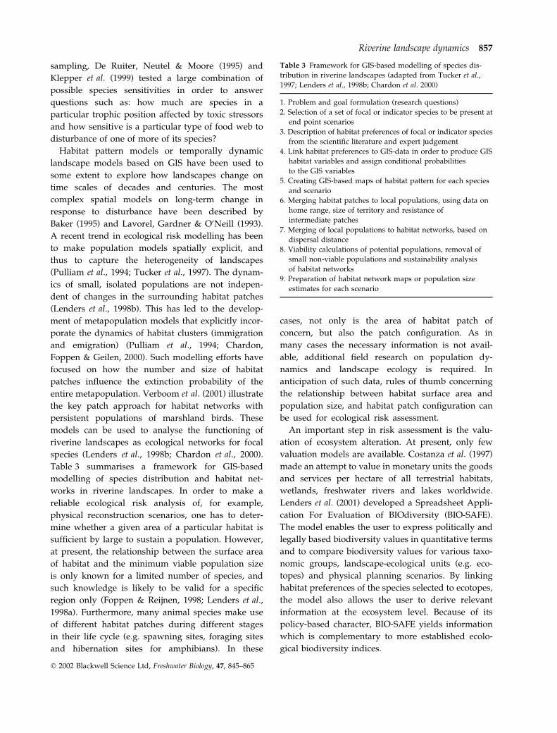
Table 3 summarises a framework for GIS-based

modelling of species distribution and habitat net-

works in riverine landscapes. In order to make a

reliable ecological risk analysis of, for example,

physical reconstruction scenarios, one has to deter-

mine whether a given area of a particular habitat is

sufficient by large to sustain a population. However,

at present, the relationship between the surface area

of habitat and the minimum viable population size

is only known for a limited number of species, and

such knowledge is likely to be valid for a specific

region only (Foppen & Reijnen, 1998; Lenders et al.,

1998a). Furthermore, many animal species make use

of different habitat patches during different stages

in their life cycle (e.g. spawning sites, foraging sites

and hibernation sites for amphibians). In these

cases, not only is the area of habitat patch of

concern, but also the patch configuration. As in

many cases the necessary information is not avail-

able, additional field research on population dy-

namics and landscape ecology is required. In

anticipation of such data, rules of thumb concerning

the relationship between habitat surface area and

population size, and habitat patch configuration can

be used for ecological risk assessment.

An important step in risk assessment is the valu-

ation of ecosystem alteration. At present, only few

valuation models are available. Costanza et al. (1997)

made an attempt to value in monetary units the goods

and services per hectare of all terrestrial habitats,

wetlands, freshwater rivers and lakes worldwide.

Lenders et al. (2001) developed a Spreadsheet Appli-

cation For Evaluation of BIOdiversity (BIO-SAFE).

The model enables the user to express politically and

legally based biodiversity values in quantitative terms

and to compare biodiversity values for various taxo-

nomic groups, landscape-ecological units (e.g. eco-

topes) and physical planning scenarios. By linking

habitat preferences of the species selected to ecotopes,

the model also allows the user to derive relevant

information at the ecosystem level. Because of its

policy-based character, BIO-SAFE yields information

which is complementary to more established ecolo-

gical biodiversity indices.

Table 3 Framework for GIS-based modelling of species dis-

tribution in riverine landscapes (adapted from Tucker et al.,

1997; Lenders et al., 1998b; Chardon et al. 2000)

1. Problem and goal formulation (research questions)

2. Selection of a set of focal or indicator species to be present at

end point scenarios

3. Description of habitat preferences of focal or indicator species

from the scientific literature and expert judgement

4. Link habitat preferences to GIS-data in order to produce GIS

habitat variables and assign conditional probabilities

to the GIS variables

5. Creating GIS-based maps of habitat pattern for each species

and scenario

6. Merging habitat patches to local populations, using data on

home range, size of territory and resistance of

intermediate patches

7. Merging of local populations to habitat networks, based on

dispersal distance

8. Viability calculations of potential populations, removal of

small non-viable populations and sustainability analysis

of habitat networks

9. Preparation of habitat network maps or population size

estimates for each scenario



Discussion and conclusion

Ecological risk assessment will not be influential until

authorities and stakeholders agree that some ecolog-

ical attributes are worth being protected or rehabilit-

ated (Suter, 2000). This agreement requires a clear

definition of the problem and the endpoints, spatial

scale and temporal horizon of ecological risk assess-

ment. Ecological risk assessment should be incorpor-

ated into a framework of general risk management

(US-EP2, 1992; Van de Guchte, 1995). According to the

U.S. Presidential/Congressional Commission on Risk

Assessment & Risk Management (1997), this frame-

work has six steps (Table 4). The present paper gives

an account of the approaches, concepts, assessment

endpoints and tools for analysing ecological risks to

riverine landscape dynamics. It is argued that estab-

lishing criteria based on cause-and-effect relation-

ships, defining acceptable limits, and linking results of

risk assessments in a decision-making framework are

of prime importance in the assessment of ecological

risks of large rivers (cf. Lowell et al., 2000).

Data requirements for ecological risk analyses of

riverine landscape dynamics are large (cf. Ramade,

1995; Lowell et al., 2000). Data were needed, for

example, on the relationships between riverine land-

scape dynamics and key ecosystem attributes

(Table 1), and on the thresholds for various anthrop-

ogenic disturbances. Assessment of whole-ecosystem

performance is inherently complex and difficult to

carry out, hence requiring sophisticated modelling

and synthesis. Assessing whole-ecosystem perform-

ance also is less precise than evaluating single indi-

cators, but because of its generally greater relevance,

whole-ecosystem assessment is typically preferable

(Costanza, 1995).

The possibility that riverine ecosystems are exposed

simultaneously or sequentially to multiple stressors

requires consideration of the interaction effects of the

stressors on organisms, ecosystems and landscapes.

However, in spite of growing interest in multiple

stressors (e.g. Lowell et al., 2000; Morton et al., 2000),

basic data are often either lacking or inadequate to

allow precise predictions at the riverine ecosystem

level (Leuven et al., 1998; Van der Velde & Leuven,

1999). Clearly, methods must be developed that

separate the effects of different stressors, their inter-

actions and any modulating factors (Williams &

Kapustka, 2000). This requires establishing the causal

relationships underlying an impact brought about by

multiple stressors. According to Lowell et al. (2000), a

weight-of-evidence approach is needed that combines

information from various sources and evaluates the

strength of causality by a formalised set of criteria

(Table 5).

In the search for general rules about the relation-

ships among species characteristics and landscape

dynamics, it has been recommended to analyse a

variety of focal species with contrasting habitat

requirements, life histories and dispersal behaviour

(Ormerod & Watkinson, 2000). Cross-system compar-

isons and retrospective analyses following a distur-

bance are useful to assess the resistance, resilience and

elasticity of riverine ecosystems for different combi-

nations of disturbances. However, at present, ecolog-

ical risk assessment relies very much on field surveys

that yield correlation between potential stressors and

presumed effects, but do not provide insight into

causal relationships.

Table 4 Framework for ecological risk management (Presiden-

tial/Congressional Commission on Risk Assessment and Risk

Management, 1997)

1. Define the problem and put it in context

2. Analyse the risks associated with the problem in context

3. Examine options (scenarios) for addressing the risks

4. Make decision about which options to implement

5. Take action to implement the decisions

6. Evaluate the action’s results

Table 5 Formalised set of causal criteria to generate weight-of-

evidence risk assessment for large rivers (Culp et al., 2000;

Lowell et al., 2000)

1. Spatial correlation of stressor and effect along gradient from

more to less exposed areas

2. Temporal correlation of stressor and effect relative to time

course of exposure

3. Plausible mechanism linking stressor and effect

4. Experimental verification of stressor effects under controlled

conditions and concordance of experimental results

with field data

5. Strength: steep exposure and response curve

6. Specificity: effect diagnostic of exposure to a particular

stressor

7. Evidence of exposure to contaminants or other stressors

8. Consistency of stressor–effect association among different

studies within the region being studied

9. Coherence with existing knowledge from other regions where

the same or analogous stressors and effects have

been studied



Remote sensing (geo)statistical techniques and GIS-

based models are important tools for incorporating

spatial and temporal components of landscape and

community attributes into ecological risk assessment.

Outputs of current ecological risk models are valu-

able, but improved validation, testing and uncertainty

analysis is clearly needed (Vose, 1996; Hope, 1999;

Williams & Kapustka, 2000). Accomplishing this task

will require considerable innovation.

Many river managers regard ecological risk assess-

ment as a tool that helps detect environmental

degradation well before the impact reaches catastro-

phic dimensions (Cairns, Niederlehner & Orvos, 1993;

Shrader-Frechette, 1998). The underlying idea is that

prevention is preferable to restoration. Once ecosys-

tems have been seriously altered, it may theoretically

be possible to restore some of their structural and

functional attributes (Aronson & Le Floc’h, 1996).

Restoration measures always entail costs, however,

whose amount depends on how early in the alteration

process the measures are applied. In the last few

decades, the engineering costs of replacing lost eco-

system services with industrial systems have indeed

proved increasingly burdensome (Cairns, 2000), and

the success of some restoration measures has been

debated. Attention should therefore be focused on the

elaboration and application of predictive models and

scenario studies (Harms & Wolfert, 1998). Forecasting

scenarios project present trends or expectations onto

the future landscape. Backcasting scenarios identify

possible alternatives and compare them with the

existing conditions in order to determine the most

desirable situation. Several types of models (or expert

systems) for ecological risk assessment of riverine

landscape dynamics (such as network analysis, eco-

toxicological and valuation models) coupled with

hydrological and geomorphologic models should be

integrated in decision support systems for integrated

assessment. These model outputs can be used for

design and evaluation of planned projects, for envi-

ronmental impact assessments and for comparative

landscape-ecological studies.

Acknowledgments

The Swiss Federal Institute for Environmental Science

and Technology (EAWAG/ETH) has provided finan-

cial support for presentation of this topical review at

the First International Symposium on Riverine Land-

scapes, 25–30 March 2001, in Ascona (Switzerland).

We thank Prof Dr P. Edwards, Dr M. Gessner, Dr K.

Tockner and two anonymous referees for valuable

comments on an earlier draft of this paper, Mr J.J.A.

Slippens for preparing drawings, Mr L. Kooistra for

providing unpublished data, and Dr A.M.J. Ragas and

Dr M.A.J. Huijbregts for stimulating discussions and

relevant references concerning ecological risk assess-

ment.

References

Aarts B.G.W. & Nienhuis P.H. (1999) Ecological sus-

tainability and biodiversity. International Journal of

Sustainable Development World Ecology, 6, 1–14.

Admiraal W., Barranguet C., Van Beusekom S.A.M.,

Bleeker E.A.J., Van den Ende F.P., Van der Geest H.G.,

Goenendijk D., Ivorra N., Kraak M.H.S. & Stuijfzand

S.C. (2000) Linking ecological and ecotoxicological

techniques to support river rehabilitation. Chemosphere,

41, 289–295.

Alard D. & Poudevigne I. (2000) Diversity patterns in

grasslands along a landscape gradient in north western

France. Journal of Vegetation Science, 11, 287–294.

Alard D. & Poudevigne I. (2002) Biodiversity in changing

landscapes: from species or patch assemblages to

system organisation. In: Application of Geographic

Information Systems and Remote Sensing in River Studies

(Eds R.S.E.W. Leuven, I. Poudevigne & R.M. Teeuw),

pp. 9–24. Backhuys Publishers, Leiden.

Alard D., Poudevigne I., Dutoit T. & Decaens T. (1998)

Dynamique de la biodiversite dans un espace en

mutation. Le cas des pelouses calcicoles de la basse

vallee de Seine. Acta Oecologica, 19, 275–284.

Aronson J. & Le Floc’h E. (1996) Vital landscape attrib-

utes: missing tools for restoration ecology. Restoration

Ecology, 4, 377–387.

Aronson J.C., Floret Le Floc’h E., Ovalle C. & Pontanier R.

(1993) Restoration and rehabilitation of degraded

ecosystems in arid and semi-arid lands. I. A view

from the south. Restoration Ecology, 1, 8–13.

Baker W.L. (1995) Long term response of disturbance

landscapes to human intervention and global change.

Landscape Ecology, 10, 143–159.

Balent G. & Courtiade B. (1992) Modelling bird commu-

nities/landscape patterns relationships in a rural area

of South-Western France. Landscape Ecology, 6, 195–211.

Balent G., Alard D., Blanfort V. & Poudevigne I. (1999)

Pratique de gestion, biodiversite floristique et durab-

ilite des prairies. Fourrages, 12, 46–52.

Blondel J. (1995) Biogeographie: Approche Ecologique et

Evolutive. Masson, Paris.



Bornette G. & Amoros C. (1996) Disturbance regimes and

vegetation dynamics: role of floods in riverine wet-

lands. Journal of Vegetation Science, 7, 615–622.

Bornette G., Amoros C., Piegay H., Tachet J. & Hein T.

(1998) Ecological complexity of wetlands within a river

landscape. Biological Conservation, 85, 35–45.

Boulton A.J. (1999) An overview of river health assess-

ment: philosophy, practice, problems and prognosis.

Freshwater Biology, 41, 469–479.

Brock T.C.M. & Budde B.J. (1994) On the choice of

structural parameters and endpoints to indicate

responses of freshwater ecosystems to pesticide stress.

In: Freshwater Field Tests for Hazard Assessment of

Chemicals (Eds J.R. Hill, F. Heimbach & F. Leeuwangh),

pp. 19–56. Lewis Publishers, London.

Burrough P.A. (1981) The fractal dimensions of land-

scapes and other environmental data. Nature, 294,

240–242.

Burrough P.A. (1993) Soil variability: a late 20th century

view. Soils and Fertilisers, 56, 529–562.

Burrough P.A. & McDonnell R.A. (1998) Principles of

Geographical Information Systems. Oxford University

Press, Oxford.

Cairns J.J. (1999) Exemtionalism vs environmentalism:

the crucial debate on the value of ecosystem health.

Aquatic Ecosystem Health and Management, 2, 331–338.

Cairns J.J. (2000) Setting restoration goals for technical

feasibility and scientific validity. Ecological Engineering,

15, 171–180.

Cairns J.J., Niederlehner B.R. & Orvos D.R. (1993)

Predicting Ecosystem Risk. Princeton Scientific Publish-

ing, Princeton.

Carlon C., Critto A., Marcomini A. & Nathanail P. (2001)

Risk based characterisation of contaminated industrial

site using multivariate and geostatistical tools.

Environmental Pollution, 111, 417–427.

Carpenter S.R., Brock W.A. & Hansen J. (1999) Ecological

and social dynamics in simple models of ecosystem

management. Conservation Ecology, 3, 121–128.

Chardon J.P., Foppen R.P.B. & Geilen N. (2000) LARCH-

RIVER: a method to assess the functioning of rivers

as ecological networks. European Water Management, 3,

35–43.

Clark J.S. (1991) Disturbance and population structure

on the shifting mosaic landscape. Ecology, 72,

1119–1137.

Clifford P.A., Barchers D.E., Ludwig D.F., Sielken R.L.,

Klingensmith J.S., Smith V. & Banton M.I. (1995) An

approach to quantifying spatial components of expo-

sure for ecological risk assessment. Environmental

Toxicology and Chemistry, 14, 895–906.

Collinge S.K. & Forman R.T.T. (1998) A conceptual model

of land conversion processes: predictions and evidence

from a micro landscape experiment with grassland

insects. Oikos, 82, 66–84.

Cook R.B., Suter G.W. & Sain E.R. (1999) Ecological risk

assessment in a large river-reservoir: Introduction and

background. Environmental Toxicology and Chemistry,

18, 581–588.

Costanza R. (1995) Ecological and economic system

health and social decision making. In: Evaluating and

Monitoring the Health of Large Scale Ecosystems (Eds D.J.

Rapport, C.L. Gaudet & P. Calow), pp. 45–72. Springer

Verlag, Berlin.

Costanza R., D’Arge R., De Groot R. et al. (1997) The

value of the world’s ecosystem services and natural

capital. Nature, 387, 253–260.

Costanza R. & Mageau M. (1999) What is a healthy

ecosystem? Aquatic Ecology, 33, 105–115.

Costanza R., Wainger L., Folke C. & Maler K.G. (1993)

Modelling complex ecological economic systems –

towards an evolutionary understanding of people

and nature. Bioscience, 43, 545–555.

Cullinan V.I. & Thomas J.M. (1992) A comparison of

quantitative methods for examining landscape pattern

and scale. Landscape Ecology, 7, 211–227.

Culp J.M., Lowell R.B. & Cash K.J. (2000) Integrating

mesocosm experiments with field and laboratory

studies to generate weight-of evidence risk assess-

ments for large rivers. Environmental Toxicology and

Chemistry, 19, 1167–1173.

Daily G. (1997) Nature’s Services: Societal Dependence

on Natural Ecosystems. Island Press, Washington,

DC.

De Groot R. (1992) Functions of Nature: Evaluation of

Nature in Environmental Planning, Management and

Decision-Making. Wolters-Noordhoff, Groningen.

De Pablo C.L., Agar P.M., Gomez Sal A. & Pineda F.D.

(1988) Descriptive capacity and indicative value

of territorial variables in ecological cartography.


De Ruiter P.C., Neutel A.M. & More J.C. (1995) Energe-

tics, patterns of interaction strengths, and stability in

real ecosystems. Science, 269, 1257–1260.

Detenbeck N.E., Batterman S.L., Brady V.J., Brazner J.C.,

Snarski V.M., Taylor D.L., Thompson J.A. & Arthur

J.W. (2000) A test of watershed classification systems

for ecological risk assessment. Environmental Toxicology

and Chemistry, 19, 1174–1181.

Dyer S.D., White-Hull C., Carr G.J., Smith E.P. &

Wang X. (2000) Bottom-up and top-down approaches

to assess multiple stressors over large geographic

areas. Environmental Toxicology and Chemistry, 19,

1066–1075.

Eriksson O. (1993) The species pool hypothesis and plant

community diversity. Oikos, 68, 371–374.



Fairweather P.G. (1999) State of environment indicators

of ‘river health’: exploring the metaphor. Freshwater

Biology, 41, 211–220.

Ferenc S.A. & Foran J.A. (2000) Multiple Stressors in

Ecological Risk and Impact Assessment: Approaches to Risk

Estimation. SETAC Press, Pensacola.

Ferguson B.K. (1996) The maintenance of landscape

health in the midst of land use change. Journal of

Environmental Management, 48, 387–395.

Findlay C.S. & Zheng L. (1999) Estimating ecosystem

risks using cross-validated multiple regression and

cross-validated holographic neural networks. Ecologi-

cal Modelling, 119, 57–72.

Foppen R.P.B. & Reijnen R. (1998) Ecological networks in

riparian systems: examples for Dutch floodplain rivers.

In: New Concepts for Sustainable Management of River

Basins (Eds P.H. Nienhuis, R.S.E.W. Leuven & A.M.J.

Ragas), pp. 35–52. Backhuys Publishers, Leiden.

Forman R.T.T. & Collinge S.K. (1997) Nature conserved

in changing landscapes with and without spatial

planning. Landscape and Urban Planning, 37, 129–135.

Godron M. & Forman R.T.T. (1983) Landscape modifica-

tion and changing ecological characteristics. In: Dis-

turbance and Ecosystems (Eds H.A. Mooney &

M. Godron), pp. 12–28. Springer-Verlag, Berlin.

Gordon S.I. & Majumder S. (2000) Empirical stressor–

reponse relationships for prospective risk analysis.

Environmental Toxicology and Chemistry, 19, 1106–1112.

Gorree M., Tamis W.L.M., Traas T.P. & Elbers M.A.

(1995) BIOMAG: a model for biomagnification in

terrestrial food chains. The case for cadmium in

the Kempen, The Netherlands. Science of the Total

Environment, 168, 215–223.

Grimm V. (1996) A down to earth assessment of stability

concepts in ecology: dreams, demands and the real

problems. Senckenbergiana Maritima, 27, 215–226.

Hanski I., Pakkala T., Kuussaari M. & Lei G. (1995)

Metapopulation persistence of an endangered butterfly

in a fragmented landscape. Oikos, 72, 21–28.

Harms W.B. & Wolfert H.P. (1998) Nature rehabilitation

for the river Rhine: a scenario approach at different

scales. In: New Concepts for Sustainable Management of

River Basins (Eds P.H. Nienhuis, R.S.E.W. Leuven &

A.M.J. Ragas), pp. 95–113. Backhuys Publishers, Leiden.

Hendriks A.J., Ma W.C., Brouns J.J., De Ruiter-Dijkman

E.M. & Gast R. (1995) Modelling and monitoring

organochlorine and heavy metal accumulation in soils,

earthworms and shrews in Rhine-delta floodplains.

Archives of Environmental Contamination and Toxicology,

29, 115–127.

Hoagland B.W. & Collins S.L. (1997) Gradient models,

gradient analysis, and hierarchical structure in plant

communities. Oikos, 78, 23–30.

Hobbs R.J. (1993) Effects of landscape fragmentation on

ecosystem processes in the western Australian wheat

belt. Biological Conservation, 64, 193–201.

Holling C.S. (1973) Resilience and stability of ecological

systems. Annual Review of Ecology and Systematics, 4,

1–23.

Holling C.S. (1987) Simplifying the complex. European

Journal of Operational Research, 30, 139.

Holling C.S. (1995) What barriers? What bridges? In:

Barriers and Bridges to the Renewal of Ecosystems and

Institutions (Eds L.H. Gunderson, C.S. Holling & S.S.

Light), pp. 3–36. Columbia University Press, New

York.

Hope B.K. (1999) Assessment of risk to terrestrial

receptors using uncertainty analysis – a case study.

Human and Ecological Risk Assessment, 5, 145–170.

Hornung M. & Reynolds B. (1995) The effects of natural

and anthropogenic environmental changes on ecosys-

tem processes at the catchment scale. Trends in Ecology

and Evolution, 10, 443–449.

Huston M.A. (1994) The coexistence of species on

changing landscapes. Biological Diversity, 3, 64–74.

Johnson L.B. & Gage S.H. (1997) Landscape approaches

to the analysis of aquatic ecosystems. Freshwater

Biology, 37, 113–132.

Jungwirth M., Muhar S. & Schmutz S. (2002)

Re-establishing and assessing ecological integrity in

riverine landscapes. Freshwater Biology, 47, 867–887.

Karr J.R. & Dudley D.R. (1981) Ecological perspective

on water quality goals. Environmental Management, 5,

55–68.

Keddy P.A. (1992) Assembly and response rules – two

goals for predictive community ecology. Journal of

Vegetation Science, 3, 157–164.

Kelly J.R. & Harwell M.A. (1990) Indicators of ecosystem

recovery. Environmental Management, 14, 527–545.

Klepper O., Traas T.P., Schouten A.J., Korthals G.W. &

De Zwart D. (1999) Estimating the effect on soil

organisms of exceeding no-observed effect concentra-

tions (NOECs) of persistent toxicants. Ecotoxicology, 8,

9–21.

Kolasa J. & Pickett S.T.A. (1989) Ecological systems and

the concept of biological organisation. Proceedings of the

National Academy of Science USA, 86/22, 8837–8841.

Kooistra L., Wehrens R., Leuven R.S.E.W. & Buydens

L.M.C. (2001a) Possibilities of VNIR spectroscopy for

the assessment of soil contamination in river flood-

plains. Analytica Chimica Acta, 446, 97–105.

Kooistra L., Leuven R.S.E.W., Wehrens R., Nienhuis P.H.

& Buydens L.M.C. (2001b) A procedure for incorpor-

ating spatial variability in ecological risk assessment of

Dutch river floodplains. Environmental Management, 28,

359–373.



Kooistra L., Leuven R.S.E.W., Wehrens R., Nienhuis

P.H. & Buydens L.M.C. (2002) GIS as a tool for

incorporating spatial variability of pollutants in eco-

logical risk assessment for floodplains along Dutch

rivers. In: Application of Geographic Information Systems

and Remote Sensing in River Studies (Eds R.S.E.W.

Leuven, I. Poudevigne & R.M. Teeuw), pp. 133–146.

Backhuys Publishers, Leiden.

Lambeck R.J. (1997) Focal species: a multispecies um-

brella for nature conservation. Conservation Biology, 11,

849–856.

Landis W.G. & McLaughlin J.F. (2000) Design criteria and

derivation of indicators for ecological position, direc-

tion, and risk. Environmental Toxicology and Chemistry,

19, 1059–1065.

Lavorel S., Gardner R.H. & O’Neill R.V. (1993) Analysis

of patterns in hierarchically structured landscapes.

Oikos, 67, 521–528.

Lawton J.H. (1999) Are there general laws in Ecology?

Oikos, 84, 177–192.

Lemly A.D. (1997) Risk assessment as an environ-

mental management tool: considerations for fresh-

water wetlands. Environmental Management, 21,

343–358.

Lenders H.J.R., Aarts B.G.W., Strijbosch H. & Van der

Velde G. (1998a) The role of reference and target

images in ecological recovery of rivers. Lines of

thought in the Netherlands. In: New Concepts for

Sustainable Management of River Basins (Eds P.H.

Nienhuis, R.S.E.W. Leuven & A.M.J. Ragas), pp.

35–52. Backhuys Publishers, Leiden.

Lenders H.J.R., Leuven R.S.E.W., Nienhuis P.H.,

Oostinga K.D. & Van den Heuvel P.J.M. (1998b)

Ecological rehabilitation of floodplains along the

middle reach of the river Waal: a prosperous future

for fauna target species? In: New Concepts for Sustain-

able Management of River Basins (Eds P.H. Nienhuis,

R.S.E.W. Leuven & A.M.J. Ragas), pp. 115–130.


Lenders H.J.R., Leuven R.S.E.W., Nienhuis P.H., De

Nooij R.J.W. & Van Rooij S.A.M. (2001) BIO-SAFE: a

method for evaluation of biodiversity values on the

basis of political and legal criteria. Landscape and Urban

Planning, 55, 119–135.

Leuven R.S.E.W., Haans J.L.M., Hendriks A.J., Lock

R.A.C. & Wendelaar Bonga S.E. (1998) Assessing

cumulative impacts of multiple stressors on river

systems. In: New Concepts for Sustainable Management

of River Basins (Eds P.H. Nienhuis, R.S.E.W. Leuven &

A.M.J. Ragas), pp. 241–259. Backhuys Publishers,

Leiden.

Leuven R.S.E.W., Poudevigne I. & Teeuw R.M. (Eds)

(2002) Application of Geographic Information Systems and

Remote Sensing in River Studies. Backhuys Publishers,

Leiden.

Levin S.A. (1976) Population dynamic models in hetero-

geneous environments. Annual Review of Ecology and

Systematics, 7, 287–310.

Levin S.A. (1992) The problem of pattern and scale in

ecology. Ecology, 73, 1943–67.

Levin S.A. (1999) Towards a science of ecological man-

agement. Conservation Ecology, 3, 6–9.

Llewellyn G.M., Kooistra L. & Curran P.J. (2001) The

red-edge of soil contaminated grassland spectra. Pro-

ceedings of 8th International Symposium on Physical

Measurements and Signatures in Remote Sensing, pp.

381–386, CNES, Toulouse.

Lowell R.B., Culp J.M. & Dube M.G. (2000) A weight-

of-evidence approach for northern river risk

assessment: integrating the effect of multiple stres-

sors. Environmental Toxicology and Chemistry, 19,

1182–1190.

Manel S., Buckton S.T. & Ormerod S.J. (2000) Testing

large-scale hypotheses using surveys: the effects of

land use on the habitats, invertebrates and birds of

Himalayan rivers. Journal of Applied Ecology, 37,

756–770.

Marinussen M.P.J.C. & Van der Zee S.E.A.T.M. (1996)

Conceptual approach to estimating the effect of home-

range size on the exposure of organisms to spatially

variable soil contamination. Ecological Modelling, 87,

83–89.

McCarthy M.A. & Lindenmayer D.B. (2000) Spatially-

correlated extinction in a metapopulation model of

Leadbeaters’ Possum. Biodiversity and Conservation, 9,

47–63.

McGarigal K. & Marks B.J. (1995) FRAGSTATS: Spatial

Pattern Analysis Program for Quantifying Landscape

Structure. USDA Forest Service General Technical

Report PNW-GTR-351, Pacific Northwest Research

Station, Portland, OR.

Mertes L.A.K. (2002) Remote sensing of riverine land-

scapes. Freshwater Biology, 47, 799–816.

Middelkoop H. & Asselman N.E.M. (1998) Spatial vari-

ability of floodplain sedimentation at the event scale in

the Rhine-Meuse delta, the Netherlands. Earth Surface

Processes and Landforms, 23, 561–573.

Miller J.N., Brooks R.P. & Croonquist M.J. (1997) Effects

of landscape patterns on biotic communities. Landscape

Ecology, 12, 137–153.

Moriarty F. & Walker C.H. (1987) Bioaccumulation in

food chains: a rational approach. Ecotoxicology and

Environmental Safety, 13, 208–215.

Morton M.G., Dickson K.L., Waller W.T., Acevedo M.F.,

Mayer F.L. & Ablan M. (2000) Methodology for the

evaluation of cumulative episodic exposure to



chemical stressors in aquatic risk assessment. Environ-

mental Toxicology and Chemistry, 19, 1213–1221.

Moss B. (2000) Biodiversity in fresh waters – an issue of

species preservation or system functioning. Environ-

mental Conservation, 27, 1–4.

Muller F. (1992) Hierarchical approaches to ecosystem

theory. Ecological Modelling, 63, 215–242.

Muller S., Dutoit T., Alard D. & Grevilliot F. (1998)

Restoration and rehabilitation of species-rich grassland

ecosystems in France: a review. Restoration Ecology, 6,

94–101.

Nebbache S., Poudevigne I., Feeny V. & Alard D. (2001)

Turbidity and nitrate transfer in karstic aquifers in

rural areas. Journal of Environmental Management, 62,

389–398.

Nienhuis P.H. & Leuven R.S.E.W. (1997) The role of the

science of ecology in the sustainable development

debate in Europe. Verhandlungen der Gesellschaft fur

Okologie, 27, 243–251.

Nienhuis P.H. & Leuven R.S.E.W. (2001) River restor-

ation and flood protection: controversy or synergism.

Hydrobiologia, 444, 85–99.

Nienhuis P.H., Leuven R.S.E.W. & Ragas A.M.J. (Eds)

(1998) New Concepts for Sustainable Management of River

Basins. Backhuys Publishers, Leiden.

Noppert F., Dogger J.W., Balk F. & Smits A.J.M. (1993)

Secondary poisoning in a terrestrial food chain: a

probabilistic approach. In: Integrated Soil and Sediment

Research: A Basis for Proper Protection (Eds H.J.P.

Eijsackers & T. Hamers), pp. 303–307. Kluwer Aca-

demic Publishers, Dordrecht.

Norris R.H. & Thoms M.C. (1999) What is river health?

Freshwater Biology, 41, 197–209.

Noss R.F. (1990) Indicators for monitoring biodiversity: a

hierarchical approach. Conservation Biology, 4, 355–364.

Noss R.F. (2000) High-risk ecosystems as foci for

considering biodiversity and ecological integrity in

ecological risk assessment. Environmental Science and

Policy, 3, 321–332.

Ormerod S.J. & Watkinson A.R. (2000) Large-scale

ecology and hydrology: an introductory perspective

from the editors of the Journal of Applied Ecology.

Journal of Applied Ecology, 37(S1), 1–5.

Palmer M.W. (1993) Putting things in even better order:

the advantages of canonical correspondence analysis.

Ecology, 74, 2215–2230.

Partel M., Zobel M., Zobel K. & Van der Maarel E. (1996)

The species pool and its relation to species richness:

evidence from Estonian plant communities. Oikos, 75,

111–117.

Pearson S.M. (1993) The spatial extent and relative

influence of landscape-level factors on wintering bird

populations. Landscape Ecology, 8, 3–18.

Peeters E.T.H.M., Gardeniers J.J.P. & Koelmans A.A.

(2000) Contribution of trace metals in structuring

in situ macroinvertebrate community composition

along a salinity gradient. Environmental Toxicology and

Chemistry, 19, 1002–1010.

Petts G.E. & Amoros C. (Eds) (1996) Fluvial Hydrosystems.

Chapman & Hall, London.

Petts G.E., Moller H. & Roux A.L. (Eds) (1989) Historical

Change of Large Alluvial Rivers: Western Europe. John

Wiley & Sons, Chichester.

Phipps M. (1981) Entropy and community pattern

analysis. Journal of Theoretical Biology, 93, 253–273.

Pickett S.T.A. & Cadenasso M.L. (1995) Landscape

ecology: spatial heterogeneity in ecological systems.

Science, 269, 331–334.

Pickett S.T.A., Kolasa J., Armesto J.J. & Collins S.L.

(1989) The ecological concept of disturbance and its

expression at various hierarchical levels. Oikos, 54,

129–136.

Poudevigne I., Van Rooij S.A.M., Morin P. & Alard D.

(1997) Dynamics of rural landscapes and their main

driving factors: a case study in the Seine valley,

Normandy, France. Landscape and Urban Planning, 38,

93–103.

Poudevigne I., Chabrerie O., Jackson A., Van der Berg S.,

Bourcier J.C. & Alard D. (2002a) Patterns of landscape

dynamics and their consequences on ecological com-

munities. In: Application of Geographic Information Sys-

tems and Remote Sensing in River Studies (Eds R.S.E.W.

Leuven, I. Poudevigne & R.M. Teeuw), pp. 183–200.


Poudevigne I., Alard D., Leuven R.S.E.W. & Nienhuis

P.H. (2002b) A system approach to river restoration: a

case study in the Lower Seine valley. Regulated Rivers:

Research and Management, 18, in press.

Pratt J.R. & Cairns J.J. (1993) Ecological risks associated

with the extinction of species. In: Predicting Ecosystem

Risk (Eds J.J. Cairns, B.R. Niederlehner & D.R. Orvos),

pp. 93–117. Princeton Scientific Co., Princeton.

Presidential/Congressional Commission on Risk Assess-

ment and Risk Management (1997) Framework for

environmental health risk management. Final Report 1.

The Presidential/Congressional Commission on Risk

Assessment and Risk Management, Washington

(http://www.riskworld.com).

Pulliam H.R., Liu J., Dunning J.B., Stuwart D.J. & Bishop

T.D. (1994) Modelling animal populations in changing

landscapes. IBIS, 137, 120–126.

Ramade F. (1995) Qualitative and quantitative criteria

defining a ‘healthy’ ecosystem. In: Evaluating and

Monitoring the Health of Large Scale Ecosystems (Eds

D.J. Rapport, C.L. Gaudet & P. Calow), pp. 43–61.

Springer Verlag, Berlin.



Rapport D.J. (1992) Evaluating ecosystem health. Journal

of Aquatic Ecosystem Health, 1, 15–24.

Reice S.T., Wissmar R.C. & Naiman R.J. (1990) Distur-

bance regimes, resilience and recovery of animal

communities and habitats in lotic ecosystems. Environ-

mental Management, 14, 647–659.

Rey Benayas J.M. & Scheiner S.M. (1993) Diversity

patterns of wet meadows along geochemical gradients

in central Spain. Journal of Vegetation Science, 4, 103–108.

Richardson C.J. (1994) Ecological functions and human

values in wetlands: a framework for assessing forestry

impacts. Wetlands, 14, 1–19.

Risser P.G. (1992) Landscape ecology approach to

ecosystem rehabilitation. Ecosystem Rehabilitation, 1,

37–46.

Scheffer M., Carpenter S., Foley J.A., Folke C. & Walker

B. (2001) Catastrophic shifts in ecosystems. Nature, 413,

591–596.

Schouten C.J.J., Rang M.C., De Hamer B.A. & Van Hout

H.R.A. (2000) Strongly polluted deposits in the Meuse

river floodplain and their effects on river management.

In: New Approaches to River Management (Eds A.J.M.

Smits, P.H. Nienhuis & R.S.E.W. Leuven), pp. 33–50.


Shrader-Frechette K.S. (1998) What risk management

teaches us about ecosystem management. Landscape

and Urban Planning, 40, 141–150.

Smits A.J.M., Nienhuis P.H. & Leuven R.S.E.W. (Eds)

(2000) New Approaches to River Management. Backhuys

Publishers, Leiden.

Sousa W.P. (1984) The role of disturbance in natural

communities. Annual Review of Ecology and Systematics,

15, 353–391.

Sparks R.E. (1995) Need for ecosystem management

of large rivers and their floodplains. Bioscience, 45,

168–182.

Sparks R.E., Braden J.B., Demissie M., Mitra P., Schneider

D.W., White D.C. & Xia R. (2000) Technical support of

public decisions to restore floodplain ecosystems: a

status report on the Illinois river project, USA. In: New

Approaches to River Management (Eds A.J.M. Smits, P.H.

Nienhuis & R.S.E.W. Leuven), pp. 225–247. Backhuys

Publishers, Leiden.

Stahl R.G., Orme-Zavaleta J., Austin K. et al. (2000)

Ecological indicators in risk assessment: workshop

summary. Human and Ecological Risk Assessment, 6,

671–677.

Stanford J.A., Ward J.V., Liss W.J., Frissell C.A., Williams

R.N., Lichatowich J.A. & Coutant C.C. (1996) A general

protocol for restoration of regulated rivers. Regulated

Rivers: Research and Management, 12, 391–413.

Stohlgren T.J., Coughenour M.B., Chong G.W., Binkley

D., Kalkhan M.A., Schell L.D., Buckley D.J. & Berry J.K.

(1997) Landscape analysis of plant diversity. Landscape

Ecology, 12, 155–170.

Suter G.W. (1993) Ecological Risk Assessment. Lewis

Publishers, Chelsea.

Suter G.W. (2000) Generic assessment endpoints are

needed for ecological risk assessment. Risk Analysis,

20, 173–178.

Tapsell S.M. (1995) River restoration: what are we

restoring to? A case study of the Ravensbourne River,

London. Landscape Research, 20, 98–111.

Ter Braak C.F.J. (1983) Principal components biplots and

alpha and beta diversity. Ecology, 64, 454–462.

Ter Braak C.F.J. (1986) Canonical correspondence analy-

sis; a new eigenvector technique for multivariate direct

analysis. Ecology, 69, 67–77.

Thioulouse J. & Chessel D. (1992) A method for recip-

rocal scaling of species tolerance and sample diversity.

Ecology, 73, 670–680.

Tockner K., Schiemer F., Baumgartner C., Kum G.,

Weigand E., Zweimuller I. & Ward J.V. (1999) The

Danube restoration project: species diversity patterns

across connectivity gradients in the floodplain system.

Regulated Rivers: Research and Management, 15, 245–258.

Townsend C.R., Scarsbrook M.R. & Doledec S. (1997) The

intermediate disturbance hypothesis, refugia, and bio-

diversity in streams. Limnology and Oceanography, 42,

938–949.

Traas T.P., Aldenberg T., Janse J.H., Brock T.C.M. &

Roghair C.J. (1995) Hazardous Concentrations for Ecosys-

tems: Calculations with CATS Models. Report 719102037.

Dutch National Institute of Public Health and Envi-

ronment (RIVM), Bilthoven, The Netherlands.

Tucker K., Rushton S.P., Sanderson R.A., Martin E.B. &

Blaiklock J. (1997) Modelling bird distribution – a

combined GIS and Bayesian rule based approach.


Turner B.L. (1994) Local faces, global flows: the role of

land use and land cover in global environmental

change. Land Degradation and Rehabilitation, 5, 71–78.

Urban D.L., O’Neill R.V. & Shugart H.H. (1987) A

hierarchical perspective can help scientists understand

spatial patterns. Bioscience, 37, 119–127.

US-EPA (1992) Framework for ecological risk assess-

ment. Risk Assessment Forum EPA 603/ R-92-001. United

States Environmental protection Agency (US-EPA),

Washington, DC.

Van de Guchte C. (1995) Ecological risk assessments of

polluted sediments. European Water Pollution Control,

5/5, 16–24.

Van de Koppel J., Herman P.M.J., Thoolen P. & Heip

C.H.R. (2001) Do alternate stable states occur in natural

ecosystems? Evidence from a tidal flat. Ecology, 82,

3449–3461.



Van den Berg M.M.H.W., Tamis W.L.M. & Van Straalen

N.M. (1998) Current advances from Europe: The food

web approach in ecotoxicological risk assessment.

Human and Ecological Risk Assessment, 4, 49–55.

Van der Maarel E. (1993) Some remarks on disturbance

and its relations to diversity and stability. Journal of

Vegetation Science, 4, 733–736.

Van der Velde G. & Leuven R.S.E.W. (1999) Polluted

river systems: monitoring and assessment of ecotoxi-

cological risks. Acta Hydrochimica Hydrobiologica, 27,

251–256.

Van Leeuwen C.J. (1990) Ecotoxicological effects assess-

ments in the Netherlands: Recent developments.

Environmental Management, 14, 779–792.

Van Leeuwen C.J. & Hermens J.L.M. (Eds) (1995) Risk

Assessment of Chemicals: An Introduction. Kluwer Aca-

demic Publishers, Dordrecht.

Veblen T.T. (1992) Regeneration dynamics. In: Plant

Succession Theory and Prediction (Eds D.C. Glenn-Levin,

R.K. Peet & T.T. Veblen), pp. 152–187. Chapman &

Hall, London.

Venterink H.O. & Wassen M.J. (1997) A comparison of six

models predicting vegetation response to hydrological

habitat change. Ecological Modelling, 101, 347–361.

Verboom J., Foppen R., Chardon P., Opdam P. &

Luttikhuizen P. (2001) Introducing the key patch

approach for habitat networks with persistent popula-

tions: an example for marshland birds. Biological

Conservation, 100, 189–101.

Vitousek P.M. (1994) Beyond global warming: ecology

and global change. Ecology, 75, 1861–1876.

Vitousek P.M., Aber J.D., Howarth R.W., Likens G.E.,

Matson P.A., Schindler D.W., Schlesinger W.H. &

Tilman D.G. (1997) Human alteration of the global

nitrogen cycle: sources and consequences. Ecological

Applications, 7, 737–750.

Vorenhout M., Van Straalen N.M. & Eijsackers H.J.P.

(2000) Assessment of the purifying function of eco-

systems. Environmental Toxicology and Chemistry, 19,

2161–2163.

Vos C.C. & Chardon J.P. (1998) Effects of habitat

fragmentation an road density on the distribution

pattern of the moor frog Rana arvalis. Journal of Applied

Ecology, 35, 44–56.

Vose D. (1996) Quantitative Risk Analysis: A Guide to

Monte Carlo Simulation Modelling. John Wiley & Sons,

Chichester.

Ward J.V. (1998) Riverine landscapes: biodiversity pat-

terns, disturbance regimes, and aquatic conservation.

Biological Conservation, 83, 269–278.

Ward J.V., Tockner K. & Schiemer F. (1999) Biodiversity

of floodplain river ecosystems: ecotones and connec-

tivity. Regulated Rivers: Research and Management, 15,

125–139.

Ward J.V., Tockner K., Arscott D.B. & Claret C. (2002)

Riverine landscape diversity. Freshwater Biology, 47,

517–539.

Weber M. & Schmid B. (1995) Reductionism, holism,

and integrated approaches in biodiversity research.

Interdisciplinary Science Reviews, 20, 49–60.

Wiens J.A. (2002) Riverine landscapes: taking land-

scape ecology into the water. Freshwater Biology, 47,

501–515.

Wiens J.A., Stenseth N.C., Van Horne B. & Ims R.A.

(1993) Ecological mechanisms and landscape ecology.

Oikos, 66, 369–380.

Williams L.R.R. & Kapustka L.A. (2000) Ecosystem

vulnerability: a complex interface with technical com-

ponents. Environmental Toxicology and Chemistry, 19,

1055–1058.

Wissel C. (1984) A universal law of the characteristic

return time near thresholds. Oecologia, 65, 101–107.

With K.A., Gardner R.H. & Turner M.G. (1997) Land-

scape connectivity and population distributions in

heterogeneous environments. Oikos, 78, 151–169.

Wu J. (1999) Hierarchy and scaling: extrapolating infor-

mation along a scaling ladder. Canadian Journal of

Remote Sensing, 25, 367–380.

Zonneveld I.S. (1990) Scope and concepts of landscape

ecology as an emerging science. In: Changing Land-

scapes: An Ecological Perspective (Eds I.S. Zonneveld &

R.T.T. Forman), pp. 1–20. Springer-Verlag, New York.

(Manuscript accepted 25 January 2002)



riverine landscape dynamics and ecological risk assessment

Documents