Risk-Taking Behavior in the Wake of Natural Disasters∗

Lisa Cameron

Monash University

Manisha Shah

University of California–Irvine

February 2011

Abstract

Globally, more and more individuals are living in a world of increasing natural disasters,and a disproportionate share of the damage caused by such environmental shocks is borne bypeople in developing countries. Three main categories of natural disasters account for 90% ofthe world’s direct losses: floods, earthquakes, and tropical cyclones. In Indonesia, the two mostcommonly occurring natural disasters are earthquakes and floods. We study whether naturaldisasters affect risk-taking behavior. We investigate this issue using experimental data fromrural Indonesian households which we collected in 2008. We play standard risk games (usingreal money) with randomly selected individuals and test whether players living in villages thathave been exposed to earthquakes or floods exhibit more risk aversion. We find that individualsin villages that suffered a flood or earthquake in the past three years exhibit more risk aversionthan individuals living in otherwise like villages that did not experience a disaster. This changein risk-taking behavior has important implications for economic development.

JEL Classification: Q54, O12, D81

∗We thank Abigail Barr, Ethan Ligon, Simon Loertscher, Mark Rosenzweig, Laura Schechter, John Strauss, andTom Wilkening for helpful comments. Lucie Tafara Moore provided excellent research assistance. We are also indebtedto Bondan Sikoki and Wayan Suriastini for assistance in the design and implementation of the survey. CorrespondingAuthor: Manisha Shah, Department of Economics, University of California–Irvine, email: m.shah@uci.edu.

Over the last decade, direct losses from natural disasters in the developing world averaged 35

billion USD annually. These losses are increasing. For example, these losses are more than eight

times greater than the losses suffered as a result of natural disasters during the 1960’s (EM-DAT,

2009). Three main categories of natural disasters account for 90% of the world’s direct losses: floods,

earthquakes, and tropical cyclones. A disproportionate share of the deaths and damage caused by

such environmental shocks is borne by people in developing countries (Kahn, 2005). Developing

countries are not necessarily more susceptible to natural disasters, but the impact is often more

severe there due to poor building practices and lack of adequate infrastructure. The enormity of

these losses has focused attention on how natural disasters can undermine developing countries

long-term efforts to attain and sustain economic growth (Freeman, 2000). This is becoming an

increasingly important issue as climate change scientists have predicted an increase in the frequency

of disasters like floods and tropical cyclones (IPCC 2001).

Natural disasters are traumatic events and it is thus likely that they affect individuals’ behavior

in the short term and possibly the longer term. We investigate the relationship between natural

disasters and individuals’ risk-taking behavior using data from experiments conducted in Indonesia

in 2008. If natural disasters affect people’s perceptions of the riskiness of their environment, then

we might expect them to exhibit more risk averse behavior after experiencing a natural disaster.

However, psychological theories suggest that individuals who already live in high risk environments

may not be particularly concerned about the addition of small independent risks or that individuals

may react emotionally (as opposed to cognitively) and exhibit more risk-loving behavior.

We find that individuals in villages that suffered a flood or earthquake in the past three years

make choices that exhibit higher levels of risk aversion compared to like individuals in villages

that did not experience a disaster. Individuals who have experienced an earthquake (flood) in the

past three years are 10 (6) percentage points less likely to be risk-loving. This is a large effect

and translates into a 58 (35) percent decrease in risk tolerance. Recent disasters affect risk-taking

behavior even after we control for the mean occurrence of earthquakes and floods over the previous

30 years. We also show that these results are not biased due to selection of residential location or

migration patterns. We explore to what extent the result is an income effect. We find that some,

but not all, of the effect is a consequence of a loss of income. The impact of natural disasters on

risk aversion is found to be mitigated when households have access to insurance mechanisms such

as remittances from people outside the home village.

The economics literature on natural disasters is relatively new. However, recent papers have

1

examined the impact of natural disasters on outcomes such as macroeconomic output (Noy, 2009),

income and international financial flows (Yang, 2008a), migration decisions (Halliday, 2006; Pax-

son and Rouse, 2008; Yang, 2008b), fertility and education investments (Baez et al., 2010; Finlay,

2009; Portner, 2008; Yamauchi et al., 2009), and even mental health (Frankenberg et al., 2008).

To our knowledge this is the first paper which attempts to examine the effect of natural disasters

on risk-taking behavior in a developing country. This is an extremely important question from a

development economics perspective as risk-taking behavior determines many crucial household de-

cisions related to savings and investment behavior (Rosenzweig and Stark, 1989), fertility (Schultz,

1997), human capital decisions (Strauss and Thomas, 1995), and technology adoption (Liu, 2010);

and natural disasters are so prevalent in many developing countries. Twenty-six percent of In-

donesian villages experienced a flood or earthquake from 2006-08 (PODES 2008). Therefore, the

results from this paper have important ramifications for various household decisions that influence

economic development.

We start with a brief description of ways in which natural disasters might affect risk-taking

behavior. We then discuss natural disasters as they occur in Indonesia, the data and the experi-

mental design, and present our main empirical results. We explore the extent to which experiencing

a natural disaster affects people’s perceptions of the probability and severity of such events. We

conclude with an examination of whether access to informal insurance mechanisms reduces risk

aversion in the face of a natural disaster and provide suggestive evidence that it does.

1 Why should natural disasters affect risk behavior?

It seems likely that natural disasters would affect individuals’ risk choices. Disasters may change

individuals’ perceptions of the risk they face. In a world of perfect information, individuals will have

accurately formed expectations as to the probability of such an event occurring. This constitutes

their estimate of background risk associated with natural disasters. In this world, although a

natural disaster imparts no new information, natural disasters affect behavior through their impact

on estimates of background risk. So, in areas where disasters are more prevalent, background risk

of this sort is higher and we might expect to see different risk-taking behavior than in areas with

lower background risk.

Alternatively, a natural disaster may constitute a “shock” that contains new information and

may cause estimates of background risk to be updated. We argue this is a more natural way to think

of a disaster. For example, it is difficult to think of the victims of recent disasters such as Hurricane

2

Katrina not being shocked by the event and reappraising the world in which they live. Similarly,

living through a large earthquake may make individuals perceive the world as a riskier place than

prior to the event. In this case, even if one controls for the long term prevalence of disasters,

recent disasters may affect risk-taking behavior. If this shock is incorporated in expectations of

background risk then it will have a long term effect on behavior. A possible alternative though

is that the “shock” associated with a disaster affects people’s expectations and behavior in the

short term. With time, the impact on their behavior dissipates (as long as they do not experience

another one).

A further way in which disasters are likely to affect risk-taking behavior is through their effect on

income and wealth. Disasters destroy physical property and reduce income-earning opportunities.

It is well established that wealth is negatively associated with risk aversion (CITE). Our data allow

us to explore all of these potential avenues below.

Even if we accept that changing perceptions of risk are the most likely vehicle for behavioral

change, theoretically the anticipated effect of these types of events on risk aversion remains unclear.

On the one hand, it seems natural that adding a mean-zero background risk to wealth should

increase risk aversion to other independent risks (Eeckhoudt et al., 1996; Guiso and Paiella, 2008;

Gollier and Pratt, 1996). Gollier and Pratt (1996) and Eeckhoudt et al. (1996) show that under

certain conditions, an addition of background risk will cause a utility maximizing individual to

make less risky choices. However, psychological evidence of diminishing sensitivity suggests that

if the level of risk is high, people may not be particularly concerned about the addition of a

small independent risk (Kahneman and Tversky, 1979). Quiggin (2003), using non-expected utility

theories based on probability weighting shows that for a wide range of risk-averse utility functions,

independent risks are complementary rather than substitutes. That is, aversion to one risk will

be reduced by the presence of an independent background risk. Gollier and Pratt (1996) and

Eeckhoudt et al. (1996) derive the necessary and sufficient restrictions on utility such that an

addition of background risk will cause a utility maximizing individual to make less risky choices.

Gollier and Pratt (1996) define this property as “risk vulnerability” and show that with such

preferences, adding background risk increases the demand for insurance.

Empirically, the evidence testing these theories is quite limited. Heaton and Lucas (2000), using

survey data from the US find that higher levels of background risk are associated with reduced

stock market participation. Guiso and Paiella (2008) show that the consumer’s environment affects

risk aversion and that individuals who are more likely to face income uncertainty or to become

3

liquidity constrained exhibit a higher degree of absolute risk aversion. Lusk and Coble (2003)

analyze individuals’ choices over a series of lottery choices in a laboratory setting in the presence

and absence of uncorrelated background risk. They find that adding abstract background risk

generates more risk aversion, although they do not find the effect to be quantitatively large.

We argue that experiencing a natural disaster provides new information on the “riskiness” of

living in a given area. While people have their underlying beliefs about the likelihood a natural

disaster will strike, we show that individuals are unable to adequately assess the underlying risk

of these types of shocks and therefore consider the experience of a disasters as providing new

information. Our empirical findings are consistent with Gollier and Pratt’s (1996) concept of risk

vulnerability—the risk associated with natural disasters reduces people’s propensity for risk-taking.

Moreover, our data show that those who have experienced a natural disaster more recently, report

significantly (and unrealistically) higher probabilities of a natural disaster occurring in the next

twelve months and expect the disaster to be more severe than those who have not experienced a

disaster. This is true even after we control for the mean occurrence of floods and earthquakes back

to 1980. These results suggest that changes in expectations following a disaster likely play a role

in explaining the differences in behavior. These changes seem not to persist. Our data suggest

that within 5 years of a disaster, individuals perceptions of the risk they face has returned to the

pre-crisis levels.

As far as we know there are no papers studying this phenomenon in a developing country where

conceivably the risks faced by individuals on a daily basis are particularly high, individuals are

extremely poor and a lowered willingness to take risks could have significant ramifications in terms

of living standards and economic development. Eckel et al. (2009) is the only paper of which we

are aware that studies this issue, and it does so in the U.S. and focuses on the short term impact

of Hurricane Katrina evacuees. Interestingly, our results differ from Eckel et al. (2009) as they find

that the evacuees exhibit risk-loving behavior. They subscribe such behavior to the emotional state

of the participants shortly after the hurricane.

2 Indonesia and natural disasters

Indonesia is particularly prone to natural disasters. It regularly experiences floods, earthquakes,

volcanic eruptions, forest fires, tropical cyclones, and landslides. In this paper we focus on the two

most commonly occurring natural disasters—floods and earthquakes. These occur most often and

affect the highest number of people in Indonesia (EM-DAT, 2009).

4

Our study site is rural East Java. The province of East Java covers approximately 48,000 square

kilometers of land and is home to approximately 35 million people making it one of the most densely

populated largely rural areas on earth with more than 700 people per square kilometer. Seventy

percent of its population live in rural areas and farming is the main occupation. The population is

predominantly muslim and ethnically Javanese with a significant Madurese minority. Village life is

largely traditional with village heads and elders playing important roles in village decision-making.

The majority of East Java is flat (0-500m above sea level) and relatively fertile. Flooding

generally occurs because water fills river basins too quickly and the rain water cannot be absorbed

fast enough. Figures 1 and 2 show that the entire province of East Java (Jawa Timur on the

map) suffers high intensity risk from both earthquakes (Figure 1) and floods (Figure 2). The

figures illustrate that no region in our East Java sample is immune from these natural disasters.

However, whether an earthquake and/or flood strikes a village in a given time period is obviously

unpredictable.

3 Data and experimental design

Our sample consists of approximately 1550 individuals spread across 120 rural communities, in six

districts of the province of East Java.1 These individuals participated in experimental games which

will be explained in detail below. The individuals were members in households that had previously

been surveyed as part of a randomized evaluation. The baseline survey was conducted in August

2008 and the experiments were conducted in October 2008. Both were conducted prior to the

program being introduced and so for our purposes constitute a random sample of the population,

except that only households with children were sampled.2 The risk game (based on Binswanger

(1980) and closely related to Eckel and Grossman (2002)) was played with an adult household

member.3 An important advantage of this game design is that it is easily comprehended by subjects

outside the usual convenient sample of university students. In addition, our sample size is much

larger than previous research using similar risk games with real stakes. The survey collected

information on the standard array of socio-economic variables, including income. A community

level survey was also administered to the village head. This survey provides one measure of natural

disasters affecting each village.

1East Java has 29 rural districts.2This is because of the focus of the evaluation.3The adult member with responsibility for sanitation decisions in the household was invited to play. This reflects

the primary purpose of the data collection, as a tool for evaluating sanitation decisions.

5

The risk game was conducted as follows. Individuals were asked to select one gamble from a

set of six possible gambles. Each gamble worked as follows. The experimenter showed the player

he had two marbles, a blue and a yellow one. He would then put the marbles behind his back and

shake them in his hands. Then he would take one marble in each hand and bring them forward

telling the player he had one marble concealed in each hand. The player would pick one hand. If

the player picked the hand containing the blue marble, she would win the amount of money shown

on the blue side of the table. If she picked the hand containing the yellow marble, the player would

win the amount of money shown on the yellow side of the table.4 Before playing the risk game,

the experimenter went through a series of examples with each player. When it was clear that the

player understood the game, money was put on the table to indicate the game for real stakes would

begin.5

The six 50-50 gamble options each player was given are summarized in Table 1. Gamble A

gives the participant a 50% chance of winning Rp10,000 and a 50% chance of winning Rp10,000,

hence it involves no risk. The risk associated with each gamble increases as the player progresses

down the table, with choice F being the riskiest. The expected values of the winnings in this game

range from Rp10,000 to Rp20,000 where the expected value also increases until choice E. Note that

Choice E and F have the same expected return, but F has a higher variance, so only a risk-neutral

or risk-loving person would take the step from E to F. In terms of the magnitude of the stakes,

one day’s wage in this region is approximately Rp10,000. Therefore, the potential winnings are

quite substantial. Players can win anywhere from one to four days income. Since the stakes are

substantial, we expect individuals to exhibit risk aversion as individuals are not expected to reveal

their risk aversion when stakes are relatively small (Arrow, 1971; Rabin, 2000).

Table 1 also summarizes the frequency of gamble choices that players made. Overall, the

distribution is quite similar to other studies that have played similar risk games (for example,

see Binswanger (1980); Barr and Genicot (2008); Cardenas and Carpenter (2008) for a review.)

Barr and Genicot (2008) play the same risk game based on Binswanger (1980) in a number of

Zimbabwean villages and interestingly, both of the tails on our distribution are slightly fatter than

their round 1 data, especially on the lower end. This heavier lower end may be consistent with the

large number of natural disasters in East Java increasing risk aversion.

4More detailed instructions for the risk game including the protocol are given in the appendix.5Only 11 players (0.70%) got the two test questions wrong. We proceeded with two more test questions for those

11 players. Four players (out of 11) still got the next two questions wrong. In 3 of the cases, we switched to anotherplayer within the same household and we did not play the risk game in one household.

6

3.1 Estimating risk aversion parameters

We calculate our risk measures using two different methods. We first use a simple measure of risk

attitudes. We define those individuals who selected choice E or F as exhibiting “risk-loving”(=1)

behavior6 and all others are defined as “non risk-loving”(=0). We choose choices E and F as they

are the riskiest choices an individual can make, and have the same expected value. This measure

does not require any assumptions about individuals utility functions. In addition, we construct

an alternate measure of risk aversion (following much of the experimental economics literature)

by estimating risk aversion parameters for each person assuming constant relative risk aversion

(CRRA) CES utility: U(c) = c(1−γ)

1−γ .

Most studies which estimate risk aversion parameters from experiments in developing countries

ignore income outside the experiment (Cardenas and Carpenter, 2008). However, an exception to

this is Schechter (2007) who defines utility over daily income plus winnings from the risk experiment

in Paraguay. In column 6 of Table 1, we generate risk aversion parameters by defining utility only

over winnings from the risk experiment. Column 7 of Table 1 follows Schechter (2007) and reports

risk-aversion parameters for each choice when utility is defined over daily income plus winnings

from the game. We generate household-specific risk-aversion intervals from the different risk game

choices and report the mean values of the upper and lower bound for each choice. Both methods

assume that the amount received is consumed. We describe the method in more detail in the

appendix.

In our regressions we take the lower bound of the risk aversion parameter as our dependent

variable. We use the lower bound of the interval as this is the most conservative estimate of

the risk aversion parameter and thus gives us an estimate which is a lower bound. Some scaling

decisions need to be made for choices E and F since the lower bounds are 0 and −∞ respectively.

To use the log of the lower bound of the risk aversion parameter as the dependent variable, we

set the value of choice F to some arbitrarily small number. We similarly set the value for choice

E which has a lower value of 0 to just above zero. Our empirical results are not sensitive to the

choice of the small number.7

6Given this is a sample or poor, rural Indonesians, these individuals are probably more correctly defined asexhibiting “risk-tolerant,” behavior however for ease of exposition we use the term risk-loving.

7Following Binswanger (1980), we can also use the log of the geometric mean of each interval as an alternativedependent variable. This avoids the need to add arbitrarily small figures to the zero amounts. The empirical resultsare qualitatively similar (results available upon request).

7

3.2 Measures of natural disaster

The main measures of natural disaster are obtained from a community level survey which was ad-

ministered to the village head in each community in 2008. Heads responded yes/no as to whether

their village had experienced an earthquake and/or flood and if yes, when it occurred. Approxi-

mately 10 percent of our villages experienced a flood or earthquake between 2005 and 2008. None

of the villages experienced both types of natural disasters during this period.

Though there is little reason to believe the village head would not provide accurate measures

of natural disaster, we employ data from PODES (Potensi Desa) data to construct alternative

measures of natural disaster for our villages. In addition, since the measure of natural disaster

described above do not measure intensity, we use the PODES data to construct two measures

of natural disaster for our villages which capture intensity. The PODES is a survey conducted

by the Indonesian Statistical Agency in every village of Indonesia every three years. Using the

2008 PODES, we generate a measure of the total value of material damage due to floods and/or

earthquakes from 2005-2008 for each village. The average amount of damage during this period was

reported as 46 million rupiah (or 4650 USD) with the maximum damage reported at approximately

122,000 USD. In addition, some of the villages in our sample experienced more than one flood.

Therefore, we also construct a continuous measure of flood (which varies from 0 to 6) for the same

time period using the PODES data. The mean number of floods for households that experienced a

flood is 1.3 floods. None of the villages experienced more than one earthquake during this period.

In addition, there were no reported deaths caused by earthquakes or floods during this period in

our sample villages. While these are disasters severe enough to cause material damage, none were

severe enough to cause death.8

Finally, we use data from the 2006, 2003, 2000, 1993, 1990, and 1983 PODES9 to construct a

historical measure of the mean number of earthquakes and floods in each of our villages. The mean

number of floods from 1980-2005 is .23 floods and the mean number of earthquake 1980-2005 is

0.22. We use these means as measures which proxy for historical occurrences of natural disasters.

We can think about these means as a measure of background risk and the occurrence of a new

natural disaster as a change in the perception of background risk.

8If we correlate natural disaster reports from village heads relative to the 2008 PODES data reports, the correlationis quite high and significant at 0.5.

9Questions about natural disaster were not asked in the 1986 and 1996 PODES.

8

3.3 Summary statistics

Summary statistics by risk game choice are presented in Table 2. Risk choices do not vary by

marital status. However, females are less likely to choose the riskier options which is consistent

with the experimental literature.10 In addition, as we might expect, younger, more educated, and

wealthier individuals are more likely to select riskier options. We define “wealth” as the sum of the

value of all assets the household owns (e.g. house, land, livestock, household equipment, jewelry,

etc.) and then take the natural log. In terms of natural disasters, the summary statistics in Table

2 indicate that individuals who have experienced an earthquake or flood in the past three years,

are less likely to choose more risky options. Further, individuals who live in villages that have

been flooded more frequently in the last three years make less risky choices. Below, we investigate

whether this remains the case once we control for a range of observable characteristics.

3.4 Potential Selection Bias

Our empirical strategy is simple. We regress the risk measure on the various natural disaster

measures, while controlling for household, individual, geographic characteristics, and district fixed

effects. We claim this is the causal effect of natural disaster on risk attitudes since the natural

disaster is an unexpected shock. Since all of rural East Java is in an earthquake and flood zone

(see Figures 1 and 2), and experts are unable to predict when and where an earthquake will occur,

no village in our sample is immune from the risk of these shocks. Flooding is also widespread in

East Java. Exposure to flooding risk is however largely governed by proximity to rivers and poor

drainage.

One obvious concern with this empirical strategy is that individuals who live in villages that

experienced earthquakes and floods in the past three years might be different from individuals who

live in villages that did not experience these natural disasters. For example, it is possible that

wealthier individuals choose to live in villages that do not experience flooding and are more likely

to choose the riskier option (because of their wealth). This could introduce a negative correlation

between flood and risk choice which is not causal. Similarly, villages that experienced a natural

disaster in the past 3 years might be different from villages which did not. For example, villages

which experienced a natural disaster might provide worse public goods than villages which did not,

again introducing a negative correlation between natural disasters and risk aversion which is not

causal.

10For a review of the literature on gender and risk, see Croson and Gneezy (2009).

9

To examine the extent of selectivity, Table 3 presents the mean and standard deviation of

many individual, household, and village characteristics by natural disaster status (columns 1-2).

Column 3 shows that marital status, age, gender, and education are not significantly different

from one another by natural disaster. Thus there is no indication of a selection effect along these

observable characteristics—those who experienced a natural disaster in the past three years are

no different to those who did not. We do find a different ethnic composition in these villages by

natural disaster as more Madurese individuals live in natural disaster villages than Javanese. This

is likely a reflection of geographic clustering of different ethnic groups and is unlikely to be related to

natural disaster activity. All of our regressions control for ethnicity. We also test various measures

of household poverty, such as whether the household participates in the conditional cash transfer

program (Keluarga Harapan), health insurance program for the poor(Askeskin), and whether they

have access to subsidized rice. None of these measures are significantly different from one another

suggesting households are equally poor across the types of villages. Since living on the river bank

is the riskiest place to live in terms of risk of flood, we also test if that differs by natural disaster

status—it does not.

In the second half of Table 3 we present summary statistics from the community level survey.

We investigate whether the extent of public good provision and program access differ across village

types since flooding is caused by poor drainage. Again we find no significant differences. Natural

disaster and non-natural disaster villages provide the same health and sanitation programs and

have similar population sizes. We do find that natural disaster villages are significantly more likely

to have a river in close proximity. All of the empirical specifications below include a variable which

indicates whether the village is on a river. If risk-averse individuals are less likely to settle in

flood-prone areas then we would expect this variable to be positive and significant. However, it is

not statistically significant in any of the specifications.

A further concern is that wealthier households choose to live in safer areas or build houses on

higher ground, implying that wealthy households will be less likely to be affected by the natural

disasters. In Table 6 we regress natural disaster on wealth and a polynomial of wealth and find no

significant relationship between the occurrence of natural disasters and wealth. We return to the

issue of wealth below.

Since village of residence in East Java is largely a function of family roots, we consider the

potential for selection bias to be relatively small. Ties to the land and community are strong,

though the potential for migration out of villages does exist.

10

3.4.1 Migration

To further examine the extent to which selectivity is likely to be a problem, we examine migration

rates by natural disaster status. Since we do not have migration rates in our data, we use data from

the first and second waves of the Indonesian Family Life Survey (IFLS). The IFLS is a panel of over

7000 Indonesian households.11 The 1993 wave provides information on natural disasters between

1990 and 1993. The 1997 wave identifies what percentage of individuals have moved between 1993

and 1997, both within the village and beyond the village. Between 1990 and 1993, 14.4 percent

of IFLS communities in rural Indonesia experienced a flood or an earthquake. In villages that

experienced a flood or an earthquake in rural Indonesia, 16.2 percent of individuals over the age of

15 (n=1752) migrated in the following 3 years versus 16.7 percent in villages that did not (n=9897).

This difference is not statistically significant (p-value=0.63).12

We also investigate the composition of migrants to check whether different types of individuals

are migrating by disaster status, thus changing the composition of rural communities. We look

at various characteristics such as age, gender, marital status, education, and employment in rural

Indonesia and test whether characteristics of migrants differ by natural disaster status. For example,

our results might be biased if we find that younger men are more likely to be migrating from disaster

areas (because they are generally more risk-loving) relative to non-disaster areas. This would imply

that more risk-averse individuals are left behind in the villages that experience disasters, biasing

our findings upward. We find that migrants from disaster villages are 25.4 years old on average

(compared to 25.7 years old in non-disaster villages), and 52.2 percent are male (compared to 53.8

percent in non-disaster villages). Therefore it is not the case that migrants from villages that

experienced disasters are more likely to be male or younger. In addition, migrants from villages

which experienced a disaster completed 3.07 years of education on average compared to 3.30 years

in non-disaster villages and 72 percent of migrants from disaster villages are currently employed

(compared to 65.2 percent in non-disaster villages). None of these differences are statistically

significant.13 The only characteristic that differs significantly across disaster and non-disaster

11IFLS 1 (1993) and IFLS 2 (1997) were conducted by RAND in collaboration with Lembaga Demografi, Universityof Indonesia. For more information, see http://www.rand.org/labor/FLS/IFLS/.

12To check the migration statistics for a sample closer to our rural East Java sample, we conduct the same analysisfor rural Java. In villages that experienced a flood or an earthquake in rural Java, 15.6 percent of individuals over theage of 15 (n=1006) migrated in the following three years versus 13.9 percent in villages that did not (n=4742). Thoughthe point estimate suggests that natural disasters may increase the likelihood of migration, again, this difference isnot statistically significant (p-value=0.16).

13The p values for these tests are age (p-value=0.84), male (p-value=0.73), education (p-value=.25), and currentlyworking (p-value=.10)

11

villages is marital status. Married individuals (both male and female) are more likely to migrate

when the village experiences a natural disaster (51.2 percent of migrants from disaster villages are

married versus 42.2 percent, p-value=0.04). Note though that our regressions indicate that being

married does not affect risk aversion. Thus compositional differences in migrants are unlikely to be

driving our results.

Finally, selectivity may operate within a village. More risk-averse households and wealthier

families may choose to live farther from the river within their community. The IFLS data show that

10.3 percent of households in flood and earthquake affected villages in rural Indonesia moved house

within the village versus 8.4 percent in villages with no disasters. This difference is statistically

significant (p=0.01) and suggests that households are more likely to move within their village

in disaster stricken villages. However, since our sample is a random sample of the community

population and our estimates are derived from cross-village comparisons, this type of selectivity

does not bias our results.14

4 Empirical results

In Table 4, we present the results from simple linear probability models where the dependent

variable is “risk-loving” (a player who selected the riskiest choices, E or F, in the risk game).15 All

specifications allow for clustering of standard errors at the village level and include district level

fixed effects. We include district fixed effects to control for any potential differences at the district

level which might affect our results such as public goods provisions, government programs, and/or

geographic differences. Column 1 does not include any individual or household level controls; in

column 2 we include age, marital status, gender, education, ethnicity, and a dummy indicating

whether the village is on a river; and in column 3 we show the full model which includes the

previous set of controls as well as a measure of wealth. While the consensus view is that absolute

risk aversion should decline with wealth, including a measure of wealth could be endogenous since

the higher returns that accompany riskier decisions may make risk-loving individuals more wealthy.

The results show wealth to be associated with riskier behavior but its inclusion in the regression

does not change our main results. In column 4 we include the mean amount of earthquakes and

floods from 1989-2005 in each village as a measure of historical background risk.

Table 4 indicates that individuals who have experienced an earthquake in the past three years

14The figures for rural Java are 8.9 percent and 7.6 percent, p-value=0.13.15The results are quantitatively similar if we estimate probit regressions.

12

are 10 percentage points less likely to choose option E or F. This is a large effect (58 percent)

since the mean of the dependent variable is 0.17. Similarly, individuals who experienced a flood

in the past three years are 6 percentage points less likely to choose option E or F. Though this

effect is slightly smaller (35 percent decrease), it is qualitatively similar. Both of these results

are statistically significant at the .01 and .05 level. As mentioned above, the variable indicating

proximity of the community to a river is insignificant and suggests that selectivity of residence on

the basis of risk attitudes is not a problem. As we might expect, women and older individuals are

less likely to be risk-loving. Wealthier individuals are more likely to be risk-loving. These results

are consistent with findings in the experimental economics literature.

In columns 5-6 of Table 4, we introduce two different measures of natural disaster from the

PODES data. Some of the villages in our sample experienced more than one flood in the past three

years. Therefore, we include the continuous measure of flood (which varies from 0 to 6) in column 4

instead of the flood dummy in columns 1-3. The results in column 4 indicate that for a one standard

deviation increase in floods (which is equivalent to one flood), individuals are two percentage points

less likely to choose option E or F. In column 5 we use a measure of the total amount of flood and

earthquake damage (in log Indonesian rupiah). Again, we find that individuals in villages with

more flood or earthquake damage, are less likely to choose the risky options. Therefore, regardless

of the measure we use, individuals who suffered an earthquake or a flood are significantly less likely

to choose the riskier options in the risk game.

Interestingly, when we control for the mean occurrence of floods and earthquakes from 1980-2005

the main results are not affected. There also seems to be an additional effect on risk-taking behavior

from the mean earthquakes. The coefficient is negative and statistically significant suggesting that

people who lived in villages that experienced an earthquake from 1980-2005 exhibit even less risk

loving behavior. The coefficient on mean floods is not statistically significant.

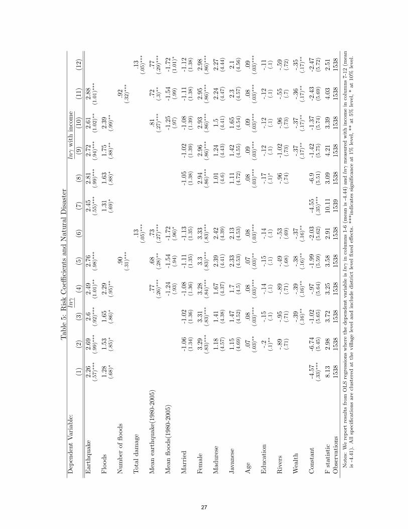
We now move to our other measures of risk, where the dependent variable is the log of the lower

bound of the relative risk aversion parameter, calculated with and without income. In columns 1-6

of Table 5, the dependent variable is calculated assuming utility is only a function of the winnings

from the game (column 6 of Table 1) and in columns 7-12 of Table 5 the dependent variable is

calculated using the winnings from the game plus household daily income (column 7 of Table 1).

We estimate OLS regressions, and all specifications allow errors to be clustered at the village level

and include district fixed effects. The control variables are the same as those described above in

Table 4, and again, we build up to the final specification which includes all control variables.

13

Overall, the results in Table 5 indicate that individuals who experience earthquakes or floods are

significantly more likely to exhibit a higher degree of risk-aversion. The magnitude of the results are

slightly difficult to interpret due to the non-linearity of the risk aversion parameters. For example,

moving from choice B to A is a 331 percent increase in the risk aversion parameter while moving

from choice C to B is a 115 percent increase. Column 3 of Table 5 displays the model with the

full set of control variables. The results indicate that experiencing an earthquake in the past three

years increases the risk parameter by 260 percent. This implies that a person who would have

chosen D is now more likely to choose the less risky option C. The maximum movement possible

given the magnitude of the effect is one choice. The coefficient on the flood variable is also positive,

though the magnitude is smaller than the earthquake coefficient. An individual who experiences a

flood will have a 165 percent larger risk parameter.

The coefficients on the control variables are also sensible. As in the previous regressions in

Table 4, females and older players are significantly more likely to have higher risk parameters (i.e.

exhibit greater risk aversion). Education is statistically significant in these regressions (until we

control for wealth in column 3), and we find that more educated players take more risk. This is

also true for the wealthier players. In columns 5-6 of Table 5, we include our alternative measures

of floods: the number of floods in the past three years and the total damage caused by earthquakes

or floods. Again, the results are consistent and statistically significant. The greater the number of

floods, the greater the risk aversion we observe in player choices. Similarly, the greater the amount

of damage caused by the floods, the greater the risk aversion.

In columns 7-12 of Table 5 we replicate the regressions in columns 1-6, however we use the

risk parameter that was generated including income in the utility function. Again individuals

who experience earthquakes or floods exhibit more risk aversion, and the results are quantitatively

similar to the results described above. In fact, the flood results are stronger and more significant.

4.1 Income Effects

One possible interpretation of our results is that the behavioral differences are driven by the changes

in income or wealth that accompany natural disasters. Note however that the specifications in Table

5 control for wealth at the time of the survey. The results also stand if we add income as a control.

(Income is not statistically significant and does not affect the other results. Results available on

request.) To examine the role played by income and wealth changes more closely we turn to another

data set. Unlike our data set, the fourth round of the Indonesian Family Life Survey (IFLS4) asked

14

households to report the value of income and assets lost due to natural disasters as well as the

amount of financial aid received (if any). The reported income lost is approximately 5 percent

of annual income.16 Once we account for financial aid received, the reported lost decreases to 2

percent of annual income.

IFLS4 respondents also played games designed to elicit risk preferences. Unlike our game, the

IFLS risk games were not played for real money. However, Table 12 shows that the IFLS data

produce similar results. We define a person as “risk-loving” if they picked the last, most risky

option in the game.17 The IFLS4 respondents played two games, which we call Game 1 and Game

2. The games differed in terms of the payoffs in the lotteries. Details are given in the appendix.18

Columns 1 and 4 show that for both games, the more disasters experienced by the household, the

more risk averse their behavior. While the magnitude of the impact of natural disasters on risk

aversion is much smaller in the hypothetical games (as expected since there are no real stakes), the

negative signs on the coefficients are consistent with our results.

Columns 2 and 5 of Table 12 include additional controls for the log of household income, log

income lost due to natural disaster, and the log of financial assistance received. This allows us

to examine if the income shock (controlling for the level of income) can explain our result. As

anticipated, the log of household per capita income is positively associated with the probability

of being risk-loving, but only significantly so for Risk Game 1.19 Total assistance received is also

positive, and again only significantly so in Game 1. Total amount lost is not significant in either

specification. In both specifications, the coefficient on the number of disasters is unaffected by the

inclusion of these controls. In column 3 and 6, we include an indicator of whether there was a large

loss of income (the top 5 percentile of amount lost). The more assistance a household receives, the

less risk averse were the choices made. Consistent with this, households that were severely affected

by the natural disaster, in terms of having lost a lot of income, act in a more risk-averse manner.

The bottom line from 12 is that although there is evidence of income effects in the data, controlling

16This is 0.004 percent of the value of household assets.17The IFLS games were Holt and Laury (2002) type risk games where respondents are asked to make choices

between a series of lottery pairs. Their choices reveal their risk preferences. The IFLS played two such games whichdiffered in terms of the stakes employed. Though not central to their results, Andrabi and Das (2010) also find thatindividuals living closer to the 2005 Pakistani earthquake fault line are significantly more risk averse when playinghypothetical risk games. We also played Holt and Laury (2002) type hypothetical risk games. The results from thehypothetical games are consistent with our main results.

18To be consistent with our sample, we limit the IFLS4 sample to rural households. We also exclude players whoanswered either of two test questions incorrectly. We also define natural disaster in a similar manner: the experienceof a flood and/or earthquake.

19Table 13 shows the results when we use wealth instead of income. Wealth is not statistically significant. Otherwisethe results are the same.

15

for both levels and changes of income does not affect our core result that experiencing a natural

disaster causes one to act in a more risk-averse manner. That is, changes in income do not fully

explain the more risk-averse behavior of households that experienced natural disasters.20

4.2 Robustness

4.2.1 Village Head Reporting Bias

One might be concerned that since the measures of natural disaster from our community survey are

reported by village heads, the heads’ characteristics might influence his or her response. Reporting

bias of this type might then bias our coefficient estimates. While we do not believe this to be the

case since the correlation between the PODES data and the data reported by village heads in the

community survey is quite high, we re-estimate our regression models controlling for village head

characteristics such as age, sex, length of tenure as village head, and education. The results are

robust to the inclusion of village head characteristics and the main estimates do not change (results

available upon request from authors).

4.2.2 Time Preferences

Another potential concern with our results is that we do not control for time preferences. To

the extent that risk preferences are correlated with discount rates, the risk aversion results could

be biased due to the omission of individuals’ discount rates. In our survey we asked standard

hypothetical questions about discounting behavior.21 From those questions we can construct a

minimum monthly discount factor for each individual. When we include the discount factor in the

regressions as an additional control variable in the regressions (from Tables 4 and 5), the main risk

aversion results do not change (results available upon request from authors). Therefore, it does not

appear to be the case that time preferences are driving the main results.

4.3 Do past disasters predict current disasters?

Our identification assumptions requires the flood or earthquake to be an unexpected shock. To the

extent floods and/or earthquakes are predictable, we would not expect their occurrence to change

risk-taking behavior. We test to see if floods from the past predict floods today and similarly

whether earthquakes from the past predict earthquakes today. The results of this exercise are

20We also control for income changes and test for an income effect by using the information on household income forthe same households in the IFLS3 2000. The coefficient on income changes is not statistically significant. Similarlywe interacted the change in income with natural disaster but again, the coefficient is not statistically significant.These results are available upon request.

21For example, “Would you prefer X today or Y in a month?” where Y is a greater amount.

16

presented in Table 7. In column 1, the dependent variable is flood occurrence in 2008 which we

regress on flood occurrence in 2007, 2006, 2005, and 1980-2005. We also include district fixed effects

and river dummies as additional control variables, and cluster standard errors at the village level.

As the results in column 1 indicate, none of the coefficients on the previous flood measures are

statistically significant. This implies that previous floods do not predict current floods. Column 2

in Table 7 presents similar regression results for earthquakes. Again, none of the coefficients are

statistically significant suggesting that past earthquakes do not predict current earthquakes.

5 Do individuals update expectations after experiencing a natural disaster?

We also asked households to report the probability (or likelihood) that a flood and/or earthquake

would occur in their village in the next year. We report the mean results of their responses by

natural disaster status in Table 3. Individuals who experienced a flood are significantly more likely

to report a higher probability that a flood will occur in the next year (42.6 vs. 12%) and slightly

(but not statistically significantly) more likely to report that an earthquake will occur in the next

year (18.2 vs. 16.8%). We also asked them to estimate how bad the impact of that flood or

earthquake would be conditional on experiencing the disaster in the next year. The responses are

coded into 5 categories with 0 being not bad at all and 4 being extremely bad and the results are

displayed in Table 3.

In Table 8 we report OLS regression results where the dependent variable is the probability that

a flood will occur (columns 1-2) regressed on year dummies for past flood experiences. All results

are clustered at the village level and include district fixed effects. Column 1 does not include

any control variables and column 2 reports results which include controls for ethnicity, gender,

age, education, marriage, rivers, and mean flood (or earthquake) occurrence from 1980-2005. In

columns 3-4 of Table 8 we report ordered probit regressions where the dependent variable is the

perceived impact of the flood if it were to occur (scale of 0-4 with 4 being the worst outcome, i.e. an

extremely bad flood and the mean for both variables is approximately 1). The results in columns

1-2 indicate that the more recent the flood experience, the more likely the individual will report a

higher probability of occurrence in the next year. Therefore, it appears that past flood experiences

suggest that individuals update (and increase) the probability that another flood will occur in the

next year. For example, a person who experienced a flood in 2008-09 reports a probability of

occurrence in the next year that is 34 points higher than an individual who did not experience a

flood in the preceding 7 years. Interestingly, this probability decreases the further away the flood

17

experience. For example, an individual who experienced a flood in 2004-05 reports a probability of

occurrence in the next year that is 23 points higher than an individual who did not experience a

flood. In 2002, the coefficient even becomes negative.22 Interestingly, this updating of expectations

occurs even after we control for the mean background risk of floods in column 2, and the mean

amount of floods over time has no impact on current day reports of expectations.

The ordered probit results in Table 8 are also very sensible. Individuals are much more likely to

report that the flood impact will be bad if they have experienced a flood in the past. In addition, we

include a dummy variable if they have experienced a bad flood in the past and it is both positive and

significant. We define a “bad flood impact” if the individual reports they had a bad or extremely

bad flood experience. This implies that an individual who experienced a bad flood in the past is

significantly more likely to report that the future flood impact will be bad.

In Table 9 we report the same regressions as in Table 8 except the measure of natural disaster

is now earthquake. The coefficients are sensible. The more recent the earthquake experience, the

higher the reported probability that an earthquake will occur in the next year. However, none of

the coefficients are statistically significant. Experiencing a bad earthquake in the past also increases

the likelihood that an individual will report that the severity of the future earthquake will be bad.

However, again the coefficients on the year dummies are not statistically significant.

These results suggest that the updating of expectations at least in part explains the more risk-

averse choices people make when they have been exposed to a disaster. Having experienced a

disaster they perceive that they now face a greater risk and greater severity of future disasters and

so are less inclined to take risks. The results in the previous section suggest this is irrational as

past experiences of floods and earthquakes have no predictive power over the occurrence of such an

event in the future. However similarly “irrational behavior” has been well-documented in different

settings. For example, “hot hand beliefs” where after a string of successes of say, calling heads

or tails to the flip of a coin, individuals believe they are on a winning streak and give subjective

probabilities of guessing the next flip correctly that are in excess of 50 percent (Croson and Sundali,

2005). The Indonesian data similarly suggests positive autocorrelation in the perceived probability

of negative events.

22We test for the equality of the year coefficients and can reject equality.

18

6 Do households self-insure?

So far the results presented are consistent with Gollier and Pratt’s (1996) definition of risk vulner-

ability. One of the implications of risk vulnerability is that individuals demand more insurance in

the presence of increased risk. We examine this using various measures of “insurance.” Given the

setting is rural Indonesia, individuals do not have access to formal earthquake or flood insurance.

However, rural households have other informal methods of self-insuring against risk.

Our data provide information on households’ participation in “arisan” and their receipt of

remittances. Arisan is the Indonesian version of rotating savings and credit associations (ROSCAs)

which are found in many developing countries. It refers to a social gathering in which a group of

friends and relatives meet monthly for a private lottery similar to a betting pool. Each member of

the group deposits a fixed amount of money into a pot, then a name is drawn and that winner takes

home the cash. After having won, the winner’s name is removed from the pot until each member

has won and the cycle is complete. The primary purpose of the arisan is to enable members to

purchase something beyond their affordability, but it is occasionally used for smoothing shocks.23

However, this is more likely when the shock is idiosyncratic (only affects a household) and much

more difficult in the presence of an aggregate shock (which affects the whole village).

In addition to arisan participation, households were asked whether they receive remittance

income from outside their village—this could be money sent from urban migrants within Indonesia

or money sent from overseas Indonesian migrants. A literature exists on the role of gifts and

remittances which households use for insurance and risk-coping strategies (Lucas and Stark, 1985;

Rosenzweig and Stark, 1989; Yang and Choi, 2007). We use arisan participation and remittance

receipt to test for informal methods of self-insurance.

In Table 10 we test whether we observe greater incidence of insurance in villages that are hit

by natural disasters. In columns 1-2, we report the mean of the insurance measure by natural

disaster status, and in column 3, we test whether the means are statistically different. Consistent

with Gollier and Pratt (1996), individuals who live in villages which experienced a natural disaster

in the previous three years are more likely to receive remittances and participate in arisan. The

amount of remittances received is also higher in villages that have experienced a natural disaster,

but not statistically significantly so.

In Table 11 we examine whether having access to insurance can reduce some of the natural

23For example, if a member falls ill, she might be given the pot of money that month even if her number was notselected.

19

disaster induced risk aversion. We regress our measures of risk on the different measures of insurance

and interact our measure of insurance and natural disaster. To the extent our results are driven by

income effects, we would expect this impact to be mitigated by insurance. Note that the analysis

presented in this section is only suggestive as the results may be biased due to endogeneity and/or

reverse causality.24

In columns 1-2 of Table 11 the dependent variable is risk-loving and in columns 4-6 the dependent

variable is the log of the lower bound of the relative risk aversion parameter. All models have errors

clustered at the village level, include district fixed effects, and include the full set of control variables.

In column 1 we report the effect of remittance receipt and arisan participation on risk aversion. The

coefficient on the interaction of natural disaster and remittance receipt is positive and statistically

significant. Receiving a remittance does provide some insurance against the impact of natural

disasters. The positive .13 coefficient almost exactly offsets the negative .14 coefficient on natural

disaster. Arisan participation however, has no statistically significant effect on on risk aversion.

Though the interaction is positive and .06, it is not statistically significant. This is consistent with

arisan being a within village insurance mechanism and so will be unable to insure villagers against

shocks that affect the whole village.

In column 2, instead of using the dummy variable for remittance receipt, we use the log amount

of remittances that a household receives (in Rp). Again, the interaction is positive and significant,

suggesting that the greater the amount received, the less risk aversion we should observe when a

natural disaster strikes.

In columns 3-4 we repeat the regressions from columns 1-2 with our alternate measure of risk

as the dependent variable. The results are very similar. Therefore, our findings are consistent with

individuals demanding more insurance when experiencing natural disasters and suggest that access

to insurance can help ameliorate some of the effect which experiencing a natural disaster has on

increased risk aversion. However, it is important to note that while insurance may offset some of

the impacts on risk aversion, it does not completely wipe out the effect. This is consistent with our

earlier results that show that income and wealth are determinants of risk-taking behavior but that

the change in wealth and/or income does not fully explain the change in behavior. These results are

consistent with DeSalvo et al. (2007) who find that 24.8% of Hurricane Katrina survivors without

24For example, remittances may be received by households that have experienced more severe disasters and so areexpected to be more risk-averse. More risk averse individuals may also seek out more insurance. Both of these effectswould however bias the coefficients against our finding that remittance receipt ameliorates the impact of naturaldisasters on risk preferences.

20

property insurance suffered from post-traumatic stress disorder versus 17.8% of those who had

property insurance (i.e. insurance had a small mitigating effect). In addition, Barr and Genicot

(2008) find that villagers in Zimbabwe are willing to make more risky choices when playing a similar

risk game when they know they have insurance.

7 Conclusion

This paper shows that individuals living in villages that have experienced a natural disaster behave

in a more risk averse manner than individuals in otherwise like villages. Our data suggest that

expectations change as a result of having experienced a natural disaster. People who have recently

experienced a disaster attach a higher probability to experiencing another in the next twelve months

and expect the impact to be more severe than people who have not experienced one. Although the

impact of disasters on risk-taking behavior is mitigated when households have access to remittances

or live in villages with access to health programs, changes in income do not fully explain the results.

Over 10 million people in Indonesia have been affected by an earthquake or a flood since

1990—this is approximately five percent of the total population (EM-DAT, 2009). That natural

disasters result in more risk-averse choices, coupled with the large number of people affected, make

this an important finding. It suggests that the adverse consequences of natural disasters stretch

beyond the immediate physical destruction of homes, infrastructure and loss of life. Increased risk

aversion very likely impairs future economic development. For example, if farmers choose less risky

technologies (as shown in Liu (2010)) or decide not to educate a child, such decisions can have

long-term consequences even if risk attitudes later rebound. While the exact longevity of these

effects is difficult to ascertain, one thing is clear. Exposure to significant damage has large impacts

on people’s risk-taking behavior that extend well beyond the year in which the disaster occurs.

The results on insurance presented above point to one potential policy solution. The provision

of insurance to counter the impact of natural disasters can partly stem this type of behavior. The

analysis also suggests that the potential benefits from infrastructure investments aimed at reducing

the likelihood of floods and mitigating the impacts of natural disasters are far higher than routinely

estimated.

Finally, in terms of theory, this paper supports Gollier and Pratt’s (1996) risk vulnerability

hypothesis and rejects the hypothesis that independent risks are complementary.

21

References

Andrabi, Tahir and Jishnu Das, “In Aid We Trust: Hearts and Minds and the Pakistan Earthquake of 2005,”World Bank Policy Research Working Paper 5440, October 2010.

Arrow, K., Essays in the Theoty of Risk-Bearing, Chicago, IL: Markham Publishing Company, 1971.

Baez, Javier, Alejandro de la Fuente, and Indhira Santos, “Do Natural Disasters Affect Human Capital? AnAssessment Based on Existing Empirical Evidence,” IZA Discussion Paper No. 5164, 2010.

Barr, Abigail and Garance Genicot, “Risk Sharing, Commitment, and Information: An Experimental Analysis,”Journal of the European Economic Association, December 2008, 6 (6), 1151–1185.

Binswanger, Hans P., “Attitudes toward Risk: Experimental Measurement in Rural India,” American Journal ofAgricultural Economics, August 1980, 62, 395–407.

Cardenas, Juan Camilo and Jeffrey Carpenter, “Behavioural Development Economics: Lessons from FieldLabs in the Developing World,” Journal of Development Studies, 2008, 44 (3), 311–338.

Croson, Rachel and James Sundali, “The Gambler’s Fallacy and the Hot Hand: Empirical Data from Casinos,”Journal of Risk and Uncertainty, 2005, 30 (3), 195–209.

and Uri Gneezy, “Gender Differences in Preferences,” Journal of Economic Literature, 2009, 47 (2), 448–474.

DeSalvo, Karen B., Amanda D. Hyre, Danielle C. Ompad, Andy Menke, L. Lee Tynes, and PaulMuntner, “Symptoms of Posttraumatic Stress Disorder in a New Orleans Workforce Following Hurricane Kat-rina,” Journal of Urban Health, 2007, 84 (2), 142–152.

Eckel, Catherine C. and Philip J. Grossman, “Sex Differences and Statistical Stereotyping in Attitudes TwoardsFinancial Risk,” Evolution and Human Behavior, 2002, 23, 281–295.

, Mahmoud A. El-Gamalb, and Rick K.Wilson, “Risk loving after the storm: A Bayesian-Network study ofHurricane Katrina evacuees,” Journal of Economic Behavior & Organization, 2009, 69, 110–124.

Eeckhoudt, L., C. Gollier, and H. Schlesinger, “Changes in Background Risk and and Risk Taking Behavior,”Econometrica, 1996, 64, 683–689.

EM-DAT, “The OFDA/CRED International Disaster Database,” Technical Report, Universite Catholique de Lou-vain, Belgium 2009.

Finlay, Jocelyn E., “Fertility Response to Natural Disasters The Case of Three High Mortality Earthquakes,”March 2009. World Bank Policy Research Working Paper 4883.

Frankenberg, Elizabeth, Jed Friedman, Thomas Gillespie, Nicholas Ingwersen, Robert Pynoos, UmarRifai, Bondan Sikoki, Alan Steinberg, Cecep Sumantri, Wayan Suriastini, and Duncan Thomas,“Mental Health in Sumatra after the Tsunami,” American Journal of Public Health, September 2008, 98 (9).

Freeman, Paul K., “Estimating Chronic Risk from Natural Disasters in Developing Countries: A Case Study onHonduras,” 2000. Working Paper.

Gollier, Christian and John W. Pratt, “Risk Vulnerability and the Tempering Effect of Background Risk,”Econometrica, September 1996, 64 (5), 1109–1123.

Guiso, Luigi and Monica Paiella, “Risk Aversion, Wealth, and Background Risk,” Journal of the EuropeanEconomic Association, December 2008, 6 (6), 1109–1150.

Halliday, Timothy, “Migration, Risk, and Liquidity Constraints in El Salvador,” Economic Development andCultural Change, July 2006, 54 (4), 893–925.

Heaton, J. and D. Lucas, “Portfolio Choice in the Presence of Background Risk,” Economic Journal, 2000, 110(460), 1–26.

Holt, Charles A. and Susan K. Laury, “Risk Aversion and Incentive Effects in Lottery Choices,” AmericanEconomic Review, December 2002, 92, 1644–55.

22

Kahn, Matthew E., “The Death Toll from Natural Disasters: The Role of Income Geography and Institutions,”The Review of Economics and Statistics, May 2005, 87 (2), 271–284.

Kahneman, Daniel and Amos Tversky, “Prospect Theory: An Analysis of Decision Under Risk,” Econometrica,1979, 47, 263–291.

Liu, Elaine, “Time to Change What to Sow: Risk Preferences and Technology Adoption Decisions of Cotton Farmersin China,” University of Houston working paper, 2010.

Lucas, Robert E.B and Oded Stark, “Motivations to Remit: Evidence from Botswana,” Journal of PoliticalEconomy, 1985, 93 (5), 901–18.

Lusk, Jayson L. and Keith H. Coble, “Risk Aversion in the Presence of Background Risk: Evidence from theLab,” 2003. Working Paper.

Noy, Ilan, “The Macroeconomic Consequences of Disasters,” Journal of Development Economics, 2009, 88, 221231.

Paxson, Christina and Cecilia Elena Rouse, “Returning to New Orleans after Hurricane Katrina,” AmericanEconomic Review Papers and Proceedings, May 2008, 98 (2), 38–42.

Portner, Claus C., “Gone with the Wind? Hurricane Risk, Fertility and Education,” February 2008. WorkingPaper.

Quiggin, J., “Background Risk in Generalized Expected Utility Theory,” Economic Theory, 2003, 22, 607–611.

Rabin, Matthew, “Risk Aversion and Expected-Utility Theory: A Calibration Theorem,” Econometrica, September2000, 68 (5), 1281–1292.

Rosenzweig, Mark and Oded Stark, “Consumption Smoothing, Migration, and Marriage: Evidence from RuralIndia,” Journal of Political Economy, 1989, 97 (4), 90526.

Schechter, Laura, “Risk Aversion and Expected-utility Theory: A Calibration Exercise,” Journal of Risk Uncer-tainty, 2007, 35, 67–76.

Schultz, T.P., “Demand for Children in Low Income Countries,” in M. R. Rosenzweig and O. Stark, eds., Handbookof Population and Family Economics, Vol. 1A, Elsevier Science B.V., 1997, pp. 349–430.

Strauss, John and Duncan Thomas, “Human Resources: Empirical Modeling of Household and Family Deci-sions,” in J. Behrman and T. N. Srinivasan, eds., Handbook of Development Economics, Vol. 3A, Elsevier Science,1995, pp. 1883–2023.

Yamauchi, Futoshi, Yisehac Yohannes, and Agnes R Quisumbing, “Natural Disasters, Self-Insurance andHuman Capital Investment : Evidence from Bangladesh, Ethiopia and Malawi,” April 2009. World Bank PolicyResearch Working Paper 4910.

Yang, Dean, “Coping with Disaster: The Impact of Hurricanes on International Financial Flows, 1970-2002,” TheB.E. Journal of Economic Analysis & Policy, 2008, 8 (1).

, “Risk, Migration, and Rural Financial Markets: Evidence from Earthquakes in El Salvador,” Social Research,Fall 2008, 75 (3), 955–992.

and HwaJung Choi, “Are Remittances Insurance? Evidence from Rainfall Shocks in the Philippines,” TheWorld Bank Economic Review, 2007, 21 (2), 219–248.

23

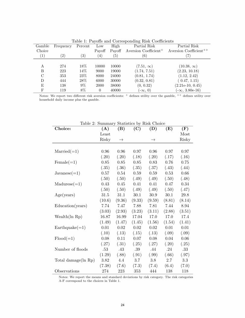
Table 1: Payoffs and Corresponding Risk CoefficientsGamble Frequency Percent Low High Partial Risk Partial RiskChoice Payoff Payoff Aversion Coefficient+ Aversion Coefficient++

(1) (2) (3) (4) (5) (6) (7)

A 274 18% 10000 10000 (7.51, ∞) (10.38, ∞)B 223 14% 9000 19000 (1.74, 7.51) (2.23, 10.18)C 353 23% 8000 24000 (0.81, 1.74) (1.12, 2.42)D 444 28% 6000 30000 (0.32, 0.81) ( 0.47, 1.15)E 138 9% 2000 38000 (0, 0.32) (2.21e-10, 0.45)F 119 8% 0 40000 (-∞, 0) (-∞, 3.80e-16)

Notes: We report two different risk aversion coefficients: + defines utility over the gamble, ++ defines utility overhousehold daily income plus the gamble.

Table 2: Summary Statistics by Risk ChoiceChoice: (A) (B) (C) (D) (E) (F)

Least MostRisky → → Risky

Married(=1) 0.96 0.96 0.97 0.96 0.97 0.97(.20) (.20) (.18) (.20) (.17) (.16)

Female(=1) 0.85 0.85 0.85 0.83 0.76 0.75(.35) (.36) (.35) (.37) (.43) (.44)

Javanese(=1) 0.57 0.54 0.59 0.59 0.53 0.66(.50) (.50) (.49) (.49) (.50) (.48)

Madurese(=1) 0.43 0.45 0.41 0.41 0.47 0.34(.50) (.50) (.49) (.49) (.50) (.47)

Age(years) 31.5 31.1 30.1 30.9 30.1 29.8(10.6) (9.36) (9.33) (9.59) (8.81) (8.14)

Education(years) 7.74 7.47 7.88 7.81 7.44 8.94(3.03) (2.93) (3.23) (3.11) (2.88) (3.51)

Wealth(ln Rp) 16.87 16.99 17.04 17.0 17.0 17.4(1.49) (1.47) (1.45) (1.56) (1.54) (1.41)

Earthquake(=1) 0.01 0.02 0.02 0.02 0.01 0.01(.10) (.13) (.15) (.13) (.09) (.09)

Flood(=1) 0.08 0.11 0.07 0.08 0.04 0.06(.27) (.31) (.25) (.27) (.20) (.25)

Number of floods .53 .43 .39 .44 .24 .33(1.29) (.88) (.91) (.99) (.66) (.97)

Total damage(ln Rp) 3.82 4.4 3.7 3.8 2.7 3.3(7.38) (7.6) (7.3) (7.4) (6.4) (7.0)

Observations 274 223 353 444 138 118

Notes: We report the means and standard deviations by risk category. The risk categoriesA-F correspond to the choices in Table 1.

24

Table 3: Summary Statistics by Natural DisasterNatural No Natural DifferenceDisaster Disaster

(1) (2) (3)

Individual and Household Characteristics:

Married(=1) 0.97 0.96 0.01(0.16) (.19)

Female(=1) 0.87 0.83 0.04(.34) (.37)

Javanese(=1) 0.49 0.58 -0.09**(.50) (.49)

Madurese(=1) 0.51 0.41 0.10**(.50) (.49)

Age(years) 29.7 30.8 -1.1(8.3) (9.6)

Education(years) 7.8 7.8 0(2.79) (3.2)

Number of friends 6.01 5.7 .30(.18) (1.41)

Has friends to borrow money .78 .75 .03(.03) (.01)

Participates in conditional cash transfer .03 .04 -.01(.01) (.01)

Health insurance for poor .24 .22 .02(.04) (.01)

Subsidized rice buyer .83 .83 0(.03) (.01)

Household on river bank .02 .02 0(.003) (.001)

Village Characteristics:

Health Care Program .47 .42 .05(.04) (.01)

Deworming Program .09 .09 0(.02) (.01)

Sanitation Program .36 .35 .01(.04) (.01)

Village population 930 999 -69(38.5) (15.5)

Has river .91 .76 .15***(.01) (.02)

Dependent Variables:

Risk-loving 0.11 0.17 -0.06*(0.32) (0.38)

ln risk aversion -3.12 -4.57 1.45(9.4) (10.7)

Probability of flood in next year 42.6 12.0 30.6***(32.4) (15.9)

Probability of earthquake in next year 18.2 16.8 1.4(18.8) (20.8)

Perceived flood impact 1.79 0.93 .86***(1.07) (0.93)

Perceived earthquake impact .84 .96 -.12(1.18) (1.3)

Observations 144 1395

Notes: We report the means and standard deviations by natural disaster. A “risk-loving”individual is someone who picked category E or F in the risk game. ***indicates differenceis statistically significant at 1% level, ** at 5% level, * at 10% level.

25

Table 4: Do Natural Disasters Affect Risk Loving?(1) (2) (3) (4) (5) (6)

Earthquake -.09 -.10 -.10 -.10 -.11(.01)∗∗∗ (.03)∗∗∗ (.03)∗∗∗ (.04)∗∗∗ (.04)∗∗∗

Flood -.05 -.06 -.06 -.08(.02)∗∗ (.03)∗∗ (.03)∗∗ (.03)∗∗

Number of floods -.03(.01)∗∗∗

Total damage -.004(.002)∗∗

Mean earthquake(1980-2005) -.03 -.02 -.03(.01)∗∗∗ (.01)∗∗ (.01)∗∗

Mean floods(1980-2005) .03 .04 .04(.03) (.03) (.04)

Married .04 .03 .04 .04 .04(.05) (.05) (.05) (.05) (.05)

Female -.11 -.11 -.11 -.12 -.12(.03)∗∗∗ (.03)∗∗∗ (.03)∗∗∗ (.03)∗∗∗ (.03)∗∗∗

Madurese .01 .00 -.01 -.03 -.03(.13) (.13) (.13) (.13) (.13)

Javanese -.01 -.02 -.03 -.05 -.04(.14) (.13) (.13) (.13) (.13)

Age -.002 -.003 -.003 -.002 -.003(.001)∗∗ (.001)∗∗ (.001)∗∗ (.001)∗∗ (.001)∗∗

Education .004 .003 .003 .003 .003(.003) (.003) (.003) (.003) (.003)

Rivers .03 .03 .03 .02 .02(.03) (.03) (.03) (.02) (.02)

Wealth .01 .01 .01 .01(.006)∗ (.006)∗ (.006)∗ (.006)∗

Constant .17 .24 .08 .08 .11 .12(.01)∗∗∗ (.17) (.18) (.18) (.18) (.18)

F statistic 29.64 5.51 3.97 4.22 3.55 2.42Observations 1539 1539 1539 1539 1539 1539

Notes: We report results from OLS regressions where the dependent variable is a dichotomous variableif the individual is risk-loving (mean is 0.17). All specifications are clustered at the village level andinclude district level fixed effects. ***indicates significance at 1% level, ** at 5% level, * at 10% level.

26

Tab

le5:

Ris

kC

oeffi

cien

tsan

dN

atu

ral

Dis

aste

rD

epen

den

tV

aria

ble

:lnγ

l nγ

wit

hin

com

e(1

)(2

)(3

)(4

)(5

)(6

)(7

)(8

)(9

)(1

0)(1

1)(1

2)

Ear

thqu

ake

2.26

2.69

2.6

2.49

2.76

2.45

2.81

2.72

2.61

2.88

(.57)∗

∗∗(.

99)∗

∗∗(.

92)∗

∗∗(1

.01)∗

∗(.

98)∗

∗∗(.

55)∗

∗∗(.

99)∗

∗∗(.

94)∗

∗∗(1

.02)∗

∗(1

.01)∗

∗∗

Flo

od

s1.2

81.5

31.

652.

291.

311.

631.

752.

39(.

68)∗

(.85)∗

(.86)∗

(.95)∗

∗(.

69)∗

(.88)∗

(.88)∗

∗(.

99)∗

∗

Nu

mb

erof

flood

s.9

0.9

2(.

31)∗

∗∗(.

32)∗

∗∗

Tot

ald

amag

e.1

3.1

3(.

05)∗

∗∗(.

05)∗

∗∗

Mea

nea

rth

qu

ake(

1980

-200

5).7

7.6

8.7

3.8

1.7

2.7

7(.

26)∗

∗∗(.

28)∗

∗(.

27)∗

∗∗(.

27)∗

∗∗(.

3)∗

∗(.

29)∗

∗∗

Mea

nfl

ood

s(19

80-2

005)

-1.2

4-1

.54

-1.7

2-1

.25

-1.5

4-1

.72

(.93)

(.94)

(.96)∗

(.97)

(.99)

(1.0

1)∗

Mar

ried

-1.0

6-1

.02

-1.0

8-1

.11

-1.1

3-1

.05

-1.0

2-1

.08

-1.1

1-1

.12

(1.3

4)

(1.3

6)

(1.3

6)

(1.3

5)

(1.3

5)

(1.3

8)

(1.3

9)

(1.3

9)

(1.3

8)

(1.3

8)

Fem

ale

3.29

3.31

3.28

3.3

3.33

2.94

2.96

2.93

2.95

2.9

8(.

83)∗

∗∗(.

83)∗

∗∗(.

84)∗

∗∗(.

83)∗

∗∗(.

83)∗

∗∗(.

86)∗

∗∗(.

86)∗

∗∗(.

86)∗

∗∗(.

86)∗

∗∗(.

86)∗

∗∗

Mad

ure

se1.1

81.

411.

672.

392.

421.

011.

241.

52.

242.2

7(4

.57)

(4.3

8)

(4.3

7)

(4.4

1)

(4.3

9)

(4.6

)(4

.43)

(4.4

1)

(4.4

7)

(4.4

4)

Jav

anes

e1.

151.

471.

72.

332.

131.

111.

421.

652.

32.1

(4.6

9)

(4.5

2)

(4.5

)(4

.53)

(4.5

3)

(4.7

2)

(4.5

5)

(4.5

4)

(4.5

7)

(4.5

6)

Age

.07

.08

.08

.07

.08

.08

.09

.09

.08

.09

(.03)∗

∗(.

03)∗

∗∗(.

03)∗

∗∗(.

03)∗

∗(.

03)∗

∗∗(.

03)∗

∗∗(.

03)∗

∗∗(.

03)∗

∗∗(.

03)∗

∗∗(.

03)∗

∗∗

Ed

uca

tion

-.2

-.15

-.14

-.15

-.14

-.17

-.12

-.12

-.12

-.11

(.1)∗

∗(.

1)

(.1)

(.1)

(.1)

(.1)∗

(.1)

(.1)

(.1)

(.1)

Riv

ers

-.89

-.95

-.89

-.49

-.53

-.96

-1.0

2-.

96

-.55

-.59

(.71)

(.71)

(.71)

(.68)

(.69)

(.74)

(.73)

(.73)

(.7)

(.72)

Wea

lth

-.39

-.39

-.38

-.37

-.37

-.37

-.36

-.35

(.16)∗

∗(.

16)∗

∗(.

16)∗

∗(.

16)∗

∗(.

17)∗

∗(.

17)∗

∗(.

17)∗

∗(.

17)∗

∗

Con

stan

t-4

.57

-6.7

4-1

.02

-.97

-1.9

9-2

.03

-4.5

5-6

.9-1

.42

-1.3

7-2

.43

-2.4

7(.

33)∗

∗∗(5

.45)

(5.6

5)

(5.6

4)

(5.5

9)

(5.6

2)

(.35)∗

∗∗(5

.51)

(5.7

5)

(5.7

4)

(5.6

9)

(5.7

2)

Fst

atis

tic

8.1

32.9

83.

723.

253.

582.

9110

.11

3.09

4.21

3.39

4.03

2.5

1O

bse

rvat

ion

s15

3815

3815

3815

3815

3815

3815

3915

3815

3815

3815

381538

Note

s:W

ere

port

resu

lts

from

OL

Sre

gre

ssio

ns

wh

ere

the

dep

end

ent

vari

ab

leislnγ

inco

lum

ns

1-6

(mea

nis

-4.4

4)

an

dlnγ

mea

sure

dw

ith

inco

me

inco

lum

ns

7-1

2(m

ean

is-4

.41).

All

spec

ifica

tion

sare

clu

ster

edat

the

villa

ge

level

an

din

clu

de

dis

tric

tle

vel

fixed

effec

ts.

***in

dic

ate

ssi

gn

ifica

nce

at

1%

level

,**

at

5%

level

,*

at

10%

level

.

27

Table 6: Do Wealthier Escape Natural Disasters?Dependent Variable: Natural Disaster

(1) (2) (3)

Wealth .005 .008 .003(.005) (.01) (.01)

Wealth squared -.001 .0001(.001) (.001)

Constant -.09 -.11 -.3(.09) (.11) (.17)∗

F statistic 2.07 1.78 .95Observations 1539 1539 1538

Notes: We report results from OLS regressionswhere the dependent variable is Natural Disaster.All specifications are clustered at the village leveland include district level fixed effects. Column 3 in-cludes additional controls for ethnicity, gender, age,education, marriage, and river dummies. ***indi-cates significance at 1% level, ** at 5% level, * at10% level.

Table 7: Do Past Natural Disasters Predict Present Natural Diasters?Dependent Variable: Flood 2008 Earthquake 2007

(1) (2)

Flood (2007) -.009(.009)

Flood (2006) .003(.004)

Flood (2005) -.009(.009)

Mean flood(1980-2005) .02(.02)

Earthquake (2006) -.04(.04)

Mean earthquake(1980-2005) .002(.002)

Constant -.01 .03(.01) (.03)

Observations 1539 1539

Notes: We report results from OLS regressions where the dependent vari-able is Flood 2008 (column 1, mean is .01) Earthquake 2007 (column2, mean is .01). All specifications are clustered at the village level andinclude district level fixed effects and river dummies. ***indicates signif-icance at 1% level, ** at 5% level, * at 10% level.

28

Table 8: Probability Flood will Occur and Perceived ImpactDependent Variable: Probability flood Perceived

will occur flood impact(1) (2) (3) (4)

Flood (2008-09) 35.29 33.78 .55 .54(8.44)∗∗∗ (8.38)∗∗∗ (.16)∗∗∗ (.16)∗∗∗

Flood (2006-07) 19.19 19.07 .14 .19(6.86)∗∗∗ (6.9)∗∗∗ (.27) (.25)

Flood (2004-05) 24.47 23.28 .58 .6(8.62)∗∗∗ (8.33)∗∗∗ (.31)∗ (.3)∗∗

Flood (2002-03) -3.41 .88 .02 .03(1.64)∗∗ (2.71) (.26) (.29)

Mean flood(1980-2005) 1.33 -.04(3.4) (.22)

Bad flood impact 1.3 1.3(.22)∗∗∗ (.21)∗∗∗

Control Variables N Y N YTest Statistic 96.0 57.4 113.7 136.4Observations 1508 1485 1505 1482

Notes: We report results from OLS regressions where the dependent vari-able is the probability that a flood will occur in the next year in columns1-2 (mean is 14.9); and ordered probit regressions where the dependentvariable is the perceived impact of the flood if it occurs in columns 3-4(mean is 1.0). All specifications are clustered at the village level and in-clude district level fixed effects. “Control Variables Y” indicates resultsinclude controls for ethnicity, gender, age, education, marriage, and rivers.***indicates significance at 1% level, ** at 5% level, * at 10% level.

Table 9: Probability Earthquake will Occur and Perceived ImpactDependent Variable: Probability earthquake Perceived

will occur earthquake impact(1) (2) (3) (4)

Earthquake (2008-09) 5.27 5.52 -.1 -.08(5.0) (5.06) (.24) (.24)

Earthquake (2006-07) 3.39 2.73 .18 .21(6.12) (5.93) (.21) (.21)

Earthquake (2004-05) -1.26 -.46 .25 .24(8.18) (7.33) (.31) (.31)

Mean earthquake(1980-2005) -.6 -.09(.77) (.14)

Bad earthquake impact 1.29 1.27(.19)∗∗∗ (.18)∗∗∗

Control Variables N Y N YTest Statistic 9.66 5.69 88.4 135.2Observations 1503 1480 1495 1472

Notes: We report results from OLS regressions where the dependent variable is the prob-ability that an earthquake will occur in the next year in columns 1-2 (mean is 16.9); andordered probit regressions where the dependent variable is the perceived impact of theearthquake if it occurs in columns 3-4 (mean is 0.95). All specifications are clustered at thevillage level and include district level fixed effects.“Control Variables Y” indicates resultsinclude controls for ethnicity, gender, age, education, marriage, and rivers. ***indicatessignificance at 1% level, ** at 5% level, * at 10% level.

29

Table 10: Insurance Measures by Natural DisasterNatural No Natural DifferenceDisaster Disaster

(1) (2) (3)

Receives remittance(=1) 0.19 0.13 0.06**(0.39) (0.34)

Remittance amount(ln Rp) 2.3 1.7 0.6(4.9) (4.6)

Participates in arisan(=1) 0.88 0.66 0.22***(.33) (.47)

Observations 144 1404

Notes: We report the means and standard deviations by natural disaster. ***indicatesdifference is statistically significant at 1% level, ** at 5% level, * at 10% level.

Table 11: Does “Insurance” Help?Dependent Variable: risk-loving lnγ

(1) (2) (3) (4)

Natural Disaster -.14 -.14 3.39 3.35(.07)∗∗ (.07)∗∗ (1.44)∗∗ (1.43)∗∗

Arisan .001 .001 -.23 -.23(.02) (.02) (.55) (.55)

Arisan*natural Disaster .05 .05 -1.18 -1.13(.07) (.07) (1.64) (1.63)

Remittance .008 -.55(.03) (.85)

Remittance*natural disaster .13 -2.58(.06)∗∗ (1.54)∗

Remittance amount .0003 -.03(.002) (.06)

Remittance amount*natural disaster .01 -.22(.004)∗∗ (.11)∗

Constant .08 .08 -1.13 -1.09(.18) (.18) (5.67) (5.66)

F statistic 2.39 2.49 2.7 2.75Observations 1547 1547 1547 1547

Notes: Notes: We report results from OLS regressions where the dependent variable isrisk-loving (columns 1-2); lnγ (columns 3-4). All specifications are clustered at the villagelevel and include controls for ethnicity, gender, age, education, marriage, wealth, river, anddistrict level fixed effects. ***indicates significance at 1% level, ** at 5% level, * at 10%level.

30

KEPULAUAN RIAU

DI YOGYAKARTA NUSA TENGGARA TIMUR

NUSA TENGGARA BARAT

SULAWESI UTARA

SULAWESI BARAT

GORONTALO

MALUKU UTARA

BANTEN

SULAWESI TENGGARA

BALI

KALIMANTAN SELATAN

NANGGROE ACEH

DARUSSALAM

BENGKULU

SUMATERA BARAT

MALUKUSULAWESI SELATAN

JAWA TENGAH

SULAWESI TENGAH

JAWA BARAT

LAMPUNG

JAWA TIMUR

SUMATERA UTARA

SUMATERA SELATAN

IRIAN JAYA BARATKALIMANTAN TENGAH

KALIMANTAN BARAT

JAMBI

KALIMANTAN TIMUR

RIAU

PAPUA

Australia

Malaysia

VietnamCambodia

PhilippinesThailand

Papua New Guinea

East Timor

Myanmar (Burma)

Brunei

India

Singapore

Pacific Islands (Palau)

Federated States of Micronesia

Cocos (Keeling) Islands

INDONESIA- UN Office for the Coordination of Humanitarian Affairs

05 March 2008

The names and boundaries on this map do not implyacceptance or official recognition by the United Nations.

Earthquake Intensity Zones

0 500 1,000250 Kilometers

LegendEarthquake IntensityModified Mercalli Scale

Degree I-VDegree VIDegree VIIDegree VIIIDegree IX-XII

The coverage as produced by the United NationsEnvironmental Programme/Global Resource Information Database (UNEP/GRID) shows earthquake intensity zonesin accordance with the 1956 version of the Modified Mercalli Scale (MM). The source of this data set is "The World Map of Natural Hazards", Munich Reinsurance Company - Geoscience Research Group (Munich Re).The intensity describes exclusively the effects of an earthquake on the surface of the earth and integrates numerous parameters (such as ground acceleration, duration of an earthquake, subsoil effects). It also includes historical earthquake reports. Therisk grading is based on expectations for a period of 50 years, corresponding to the mean service life of modern buildings.

Earthquake Intensity Risk Zones

Figure 1: Earthquake Intensity

KEPULAUAN RIAU

DI YOGYAKARTA NUSA TENGGARA TIMUR

NUSA TENGGARA BARAT

SULAWESI UTARA

SULAWESI BARAT

GORONTALO

MALUKU UTARA

BANTEN

SULAWESI TENGGARA

BALI

KALIMANTAN SELATAN

NANGGROE ACEH

DARUSSALAM

BENGKULU

SUMATERA BARAT

MALUKUSULAWESI SELATAN

JAWA TENGAH

SULAWESI TENGAH

JAWA BARAT

LAMPUNG

JAWA TIMUR

SUMATERA UTARA

SUMATERA SELATAN

IRIAN JAYA BARATKALIMANTAN TENGAH

KALIMANTAN BARAT

JAMBI

KALIMANTAN TIMUR

RIAU

PAPUA

Australia

Malaysia

VietnamCambodia

PhilippinesThailand

Papua New Guinea

East Timor

Myanmar (Burma)

Brunei

India

Singapore

Pacific Islands (Palau)

Federated States of Micronesia

Cocos (Keeling) Islands

INDONESIA- UN Office for the Coordination of Humanitarian Affairs

05 March 2008

The names and boundaries on this map do not implyacceptance or official recognition by the United Nations.

Flooding: 1985 - 2005Twenty years of flooding in the regionThis map shows flood risk in Indoensia by overlayingtwenty years of historical flood data compiled by Dartmouth Flood Observatory. Data are compiled from media and satellite remote sensing platforms. NOTE: Floods in mountaiouns regions are high energyand thus exceptionally hazardous, but they are dufficult remote sensing targets and not always observable. Additionally, cloud cover or other constraints somestimes restrict the ability to capture peak inundation. The maps are thus incomplete and do not illustrate all areas of possible flood hazard

0 500 1,000250 Kilometers

Figure 2: Flood Intensity

31

Appendix

In order to estimate a risk coefficient for each person we implement the following method. If a

person chose B then we assume she prefers B to all other choices (A, C, D, E, F). Starting with

the knowledge that she prefers B to A we have:

U(B) ≥ U(A) ⇔ U(B)− U(A) ≥ 0 (1)

If we assume a constant risk aversion (CRRA) utility function this becomes:

0.5(19000(1−γ)

(1− γ)) + 0.5(

9000(1−γ)

(1− γ))− (

10000(1−γ)

(1− γ)) ≥ 0 (2)

Where γ is the Arrow-Pratt coefficient of relative risk aversion defined as:

−CU′′(C)

U ′(C)(3)

The solution is 7.51. Therefore we conclude that the solution to the above inequality is γ ≤ 7.51

Similarly given we know that she prefers B to C we have:

U(B) ≥ U(C) ⇔ U(B)− U(C) ≥ 0 (4)

Again, if we assume a constant risk aversion (CRRA) utility function this becomes:

0.5(19000(1−γ)

(1− γ)) + 0.5(

9000(1−γ)

(1− γ))− 0.5(

24000(1−γ)

(1− γ))− 0.5(

8000(1−γ)

(1− γ)) ≥ 0 (5)

The solution is 1.74. We find that an estimate for the coefficient of relative risk aversion for

a person who chose B is such that 1.74 ≤ γ ≤ 7.51. We use the same method to estimate the

coefficient of relative risk aversion for all choices.

32

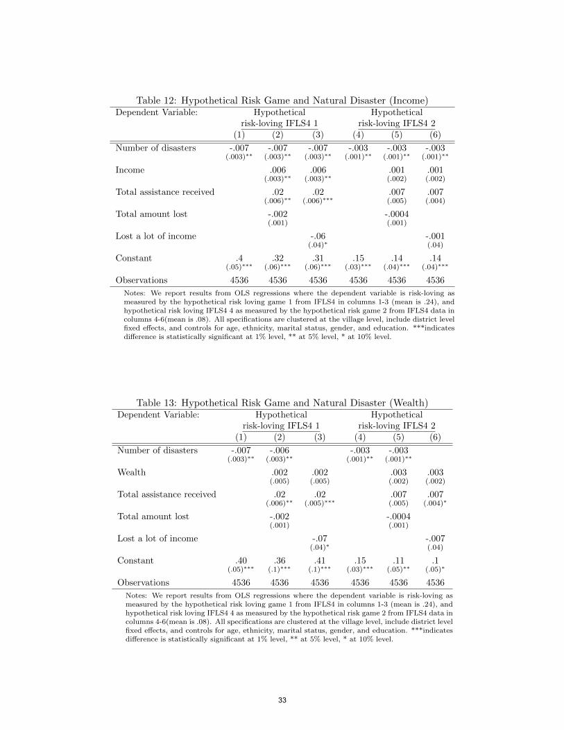
Table 12: Hypothetical Risk Game and Natural Disaster (Income)Dependent Variable: Hypothetical Hypothetical

risk-loving IFLS4 1 risk-loving IFLS4 2(1) (2) (3) (4) (5) (6)

Number of disasters -.007 -.007 -.007 -.003 -.003 -.003(.003)∗∗ (.003)∗∗ (.003)∗∗ (.001)∗∗ (.001)∗∗ (.001)∗∗

Income .006 .006 .001 .001(.003)∗∗ (.003)∗∗ (.002) (.002)

Total assistance received .02 .02 .007 .007(.006)∗∗ (.006)∗∗∗ (.005) (.004)

Total amount lost -.002 -.0004(.001) (.001)

Lost a lot of income -.06 -.001(.04)∗ (.04)

Constant .4 .32 .31 .15 .14 .14(.05)∗∗∗ (.06)∗∗∗ (.06)∗∗∗ (.03)∗∗∗ (.04)∗∗∗ (.04)∗∗∗

Observations 4536 4536 4536 4536 4536 4536

Notes: We report results from OLS regressions where the dependent variable is risk-loving asmeasured by the hypothetical risk loving game 1 from IFLS4 in columns 1-3 (mean is .24), andhypothetical risk loving IFLS4 4 as measured by the hypothetical risk game 2 from IFLS4 data incolumns 4-6(mean is .08). All specifications are clustered at the village level, include district levelfixed effects, and controls for age, ethnicity, marital status, gender, and education. ***indicatesdifference is statistically significant at 1% level, ** at 5% level, * at 10% level.

Table 13: Hypothetical Risk Game and Natural Disaster (Wealth)Dependent Variable: Hypothetical Hypothetical

risk-loving IFLS4 1 risk-loving IFLS4 2(1) (2) (3) (4) (5) (6)

Number of disasters -.007 -.006 -.003 -.003(.003)∗∗ (.003)∗∗ (.001)∗∗ (.001)∗∗

Wealth .002 .002 .003 .003(.005) (.005) (.002) (.002)

Total assistance received .02 .02 .007 .007(.006)∗∗ (.005)∗∗∗ (.005) (.004)∗

Total amount lost -.002 -.0004(.001) (.001)

Lost a lot of income -.07 -.007(.04)∗ (.04)

Constant .40 .36 .41 .15 .11 .1(.05)∗∗∗ (.1)∗∗∗ (.1)∗∗∗ (.03)∗∗∗ (.05)∗∗ (.05)∗

Observations 4536 4536 4536 4536 4536 4536

Notes: We report results from OLS regressions where the dependent variable is risk-loving asmeasured by the hypothetical risk loving game 1 from IFLS4 in columns 1-3 (mean is .24), andhypothetical risk loving IFLS4 4 as measured by the hypothetical risk game 2 from IFLS4 data incolumns 4-6(mean is .08). All specifications are clustered at the village level, include district levelfixed effects, and controls for age, ethnicity, marital status, gender, and education. ***indicatesdifference is statistically significant at 1% level, ** at 5% level, * at 10% level.

33