risk aversion, wealth, and background risk · risk aversion, wealth, and background risk ... (even...
TRANSCRIPT

RISK AVERSION, WEALTH, ANDBACKGROUND RISK
Luigi GuisoEuropean University Institute,Ente Luigi Einaudi
Monica PaiellaUniversity of Naples Parthenope
AbstractWe use household survey data to construct a direct measure of absolute risk aversion based onthe maximum price a consumer is willing to pay for a risky security. We relate this measureto consumer’s endowments and attributes and to measures of background risk and liquidityconstraints. We find that risk aversion is a decreasing function of the endowment—thus rejectingCARA preferences. We estimate the elasticity of risk aversion to consumption at about 0.7,below the unitary value predicted by CRRA utility. We also find that households’ attributesare of little help in predicting their degree of risk aversion, which is characterized by massiveunexplained heterogeneity. We show that the consumer’s environment affects risk aversion.Individuals who are more likely to face income uncertainty or to become liquidity constrainedexhibit a higher degree of absolute risk aversion, consistent with recent theories of attitudestoward risk in the presence of uninsurable risks. (JEL: D1, D8)
1. Introduction
The relationship between wealth and a consumer’s attitude toward risk—as indi-cated, for instance, by the degree of absolute risk aversion or of absolute risktolerance—is central to many fields of economics. As argued by Kenneth Arrowmore than 35 years ago, “the behavior of these measures as wealth varies is ofthe greatest importance for prediction of economic reactions in the presence ofuncertainty” (1970, p. 35).
The editor in charge of this paper was Jordi GalíAcknowledgments: We thank Chris Carroll, Pierre-André Chiappori, Christian Gollier, MichaelisHaliassos, Winfried Koeniger, Wilko Letterie, John Pratt, Andrea Tiseno, and Richard Zeckhauserfor very valuable discussion and suggestions. We are greateful to the referees and the editor fortheir comments. We are also grateful for the helpful comments of participants in seminars in Bir-beck College, City University London, European University Institute, University of Leuven, EnteLuigi Einaudi, Rand Corporation, Universidad Carlos III, the TMR conference “Savings, Pensions,and Portfolio Choice,” Deidesheim, the NBER 2000 Summer institute “Aggregate Implications ofMicroeconomic Consumption Behavior,” and the 27th EGRIE meeting. Luigi Guiso acknowledgesfinancial support from MURST and the EEC. Cristiana Rampazzi and Raghu Suryanarayanan haveprovided excellent research assistantship.E-mail: Guiso: [email protected]; Paiella: [email protected]
Journal of the European Economic Association December 2008 6(6):1109–1150© 2008 by the European Economic Association

1110 Journal of the European Economic Association
Most inference on the nature of this relation is based on common sense,introspection, casual observation of behavioral differences between the rich andthe poor, and a priori reasoning. Such inference concerns the sign of the relation,but there is no (even indirect) evidence concerning its curvature. The consensusview is that absolute risk aversion should decline with wealth.1 Furthermore, ifone agrees that preferences are characterized by constant relative risk aversion (aproperty of one of the most commonly used utility functions, the isoelastic), thenabsolute risk aversion is decreasing and convex in wealth, while risk tolerance isincreasing and linear. The curvature of absolute risk tolerance has been shownto be relevant in a number of contexts. For example, Gollier and Zeckhauser(2002) show that it determines whether the portfolio share invested in risky assetsincreases or decreases over the consumer life cycle, an issue that is receivingincreasing attention. If risk tolerance is concave, then wealth inequality can helpelucidate the risk premium puzzle (Gollier 2001). Furthermore, the curvatureof risk tolerance and the nature of risk aversion may explain why the marginalpropensity to consume out of current resources declines as the level of resourcesincreases (Carroll and Kimball 1996; Gollier 2001) even as the elasticity of risktolerance to the endowment influences the size of the precautionary saving motive(Kimball and Weil 2004).
The aim of this paper is to provide empirical evidence on the nature ofthe relationship between risk aversion and wealth. Using data from the Bankof Italy Survey of Household Income and Wealth (SHIW) on household will-ingness to pay for a hypothetical risky security, we recover a measure of theArrow–Pratt index of absolute risk aversion of the consumer lifetime utilityfunction. We then relate it to indicators of consumer endowment and alsoto a set of demographic characteristics as a control for individual preferenceheterogeneity.
Our findings show that absolute risk tolerance is an increasing function ofconsumers’ resources, thus rejecting constant absolute risk aversion (CARA)preferences. We estimate that the elasticity of absolute risk tolerance to con-sumers’ resources is between 0.6 and 0.75. This value is smaller than that impliedby constant relative risk aversion (CRRA) preferences and suggests that risk tol-erance is a concave function of wealth. This result is robust to accounting forendogeneity of the endowment and for unobserved cognitive ability. When weinstrument the measure of the endowment with exogenous variation in the educa-tion of the household head’s father and with windfall gains, the estimated elasticityis only marginally different than the OLS estimate. We also show that our resultsare unaffected by different interpretations of the hypothetical security question
1. It is on these grounds that quadratic and exponential utility, though often analytically convenient,are regarded as misleading representations of preferences; the first implies increasing absolute riskaversion and the second posits constant absolute risk aversion.

Guiso and Paiella Risk Aversion, Wealth, and Background Risk 1111
or by the presence of classical measurement error in the household’s willingnessto pay for the security.
The usual definition of risk aversion and tolerance developed by Arrow (1970)and Pratt (1964) is based on the assumption that initial wealth is nonrandom.This definition is also constructed in a static setting or in settings where fullaccess to the credit market is assumed. Recently it has been shown that attitudestoward risk can be affected by the prospect of being liquidity constrained andby the presence of additional uninsurable, nondiversifiable risks. For instance,Gollier (2000) shows that consumers who may be subject to future liquidityconstraints are less willing to bear present risks (i.e., their risk aversion increases).Moreover, depending on the structure of preferences, the presence of risks thatcannot be avoided or insured against (background risks) may make individualsless tolerant toward other, avoidable risks (Pratt and Zeckhauser 1987; Kimball1993; Eekhoudt, Gollier, and Schlesinger 1996). One important consequence isthat individuals facing high exogenous labor income risk—which is normallyuninsurable—will be more risk averse and will thus avoid exposure to portfoliorisk by holding less or no risky assets.
The evidence presented in this paper sheds light also on the empiricalrelevance of these concepts. The availability of information on measures of back-ground risk and on proxies of borrowing constraints allows us to relate our indexof risk aversion to indicators of income-related risk and of liquidity constraints.
We find that risk aversion is positively affected by background risk andalso by the possibility of being credit constrained. The effects of backgroundrisk and exposure to liquidity constraints on household willingness to bearrisk are also economically relevant: Increasing our measure of background riskby a single standard deviation lowers absolute risk tolerance by about 19%;being liquidity constrained lowers it by 4.4%. Overall, however, our estimatessuggest that these variables can explain only a small amount of the samplevariability in attitudes toward risk. Even after controlling for individual exoge-nous characteristics (e.g., age, gender, region of birth) there remains a largeamount of unexplained variation that reflects, in part, genuine differences intastes.
The rest of the paper is organized as follows. Section 2 describes our measureof risk aversion when wealth is nonrandom and when there is background risk.Section 3 presents descriptive evidence on absolute risk aversion in our cross-section of households. In Section 4 we discuss the empirical specification usedto relate absolute risk aversion to the consumer’s endowment, attributes, andenvironment. Section 5 presents the results of the estimates. In Section 6 we checkthe robustness of the main findings with respect to the endogeneity of consumptionand wealth, to nonresponses, and to the possible presence of outliers. Section 7presents evidence regarding the effects of background risk on the propensity tobear risk. Section 8 discusses the consistency with observed behavior of our

1112 Journal of the European Economic Association
findings on the shape of the wealth–risk aversion relation. Section 9 summarizesand concludes.
2. Measuring Risk Aversion
2.1. No Background Risk
To measure absolute risk aversion and tolerance, we exploit the 1995 waveof the SHIW, which is run biannually by the Bank of Italy. The 1995 SHIWcollects data on income, consumption, real and financial wealth, and severaldemographic variables for a representative sample of 8,135 Italian households.Balance-sheet items are end-of-period values. Income and flow variables referto 1995.2
The 1995 survey has a section designed to elicit attitudes toward risk. Eachparticipant is offered a hypothetical security and is asked to report the maximumprice that he would be willing to pay for it. Specifically:
We would like to ask you a hypothetical question that we would like you toanswer as if the situation was a real one. You are offered the opportunity ofacquiring a security permitting you, with the same probability, either to gain10 million lire or to lose all the capital invested. What is the most that you areprepared to pay for this security?
Ten million lire corresponds to just over 5,000 (or roughly $6,500). The ratioof the expected gain from the investment to average household total consumptionis 16%; thus, the investment represents a relatively large risk. We consider thisas an advantage, because expected utility maximizers behave as risk-neutral indi-viduals with respect to small risks even if they are averse to larger risks (Arrow1970). Thus, presenting consumers with a relatively large investment is a betterstrategy for eliciting risk attitudes when one relies (as we do) on expected utilitymaximization to characterize risk aversion.3 The interviews are conducted per-sonally at the consumer’s home by professional interviewers. In order to helpthe respondent understand the question, the interviewers show an illustrative cardand are ready to provide explanations. The respondent can answer in one of threeways: (i) declare the maximum amount he is willing to pay for the security, whichwe denote Zi ; (ii) don’t know; (iii) unwilling to answer.
2. See the Appendix for a detailed description of the survey contents, its sample design, interviewingprocedure, and response rates.3. In this vein, Rabin (2000) argues that if an expected utility maximizer refuses a small risk at alllevels of wealth than he must exhibit unrealistic levels of risk aversion when faced with large-scalerisks. This again suggests that offering large investments is a better way to characterize the riskaversion of expected utility maximizers.

Guiso and Paiella Risk Aversion, Wealth, and Background Risk 1113
Notice that the hypothetical security’s design is such that with probability1/2 the respondent gets 5,000 and with probability 1/2 he loses Zi . So theexpected value of the security is (5000 − Zi)/2. Clearly Zi < 5000, Zi = 5000,and Zi > 5000 euros imply (respectively) risk aversion, risk neutrality, andrisk loving. This characterizes attitudes toward risk qualitatively. But we cando more: within the expected utility framework, a measure of the Arrow–Prattindex of absolute risk aversion can be obtained for each consumer. Let wi denotehousehold i’s endowment, which for the moment we assume to be nonrandom. Letui(·) be the (lifetime) utility function and let Pi be the security random return forindividual i, taking values 5000 and −Zi with equal probability. The maximumpurchase price is thus given by
ui(wi) = 1
2ui(wi + 5000) + 1
2ui(wi − Zi) = Eui(wi + Pi), (1)
where E is the expectations operator.One way to derive a measure of the implied risk aversion would be to take a
second-order Taylor expansion of the second equality in equation (1) around wi
and then obtain an estimate of the Arrow–Pratt measure of absolute risk aversionin terms of the parameters of the hypothetical security of the survey. The problemwith this approach is that the risk aversion at low levels of the price Zi would begreatly underestimated, biasing toward zero the estimated relation between riskaversion and the consumer’s endowment.4
In order to avoid this problem, we assume a specific functional form for theutility function such that the coefficient of absolute risk aversion tends to infinityas the maximum reported price tends to zero; we use this form to compute theimplied absolute risk aversion for each individual in the sample. Note that we usethe specific functional form only for mapping the reported willingness to pay intoa measure of risk aversion. Ultimately, we are interested in the relation betweenrisk aversion and the consumer’s endowment, which is determined not by thespecific utility function used for the mapping but rather by the relation betweenthe reported price and the level of the individual endowment. In other words, theassumed utility function is instrumental only to avoid the bias in the estimated
4. To see this, observe that the second-order Taylor expansion of the right-hand side of equation(1) around wi gives
Eui(wi + Pi )
�
ui(wi) + u′i (wi)E(Pi) + 0.5u′′
i (wi)E(Pi)2.
Substituting this expression into equation (1) and simplifying, the measure of absolute risk aversion,Ri(wi), will be
Ri(wi)
�− u′′i (wi)/u
′i (wi) = 2(5000 − Zi)/
(50002 + Z2
i
).
As Z approaches zero, this measure of R tends to 0.2, whereas the true measure of risk aversiontends to infinity.

1114 Journal of the European Economic Association
risk aversion that would result from a second-order Taylor approximation ofequation (1); it has no effect on the relation between endowment and absoluterisk aversion. To make this point more precise, observe that the elasticity ofabsolute risk aversion to the endowment, d log R/d log w, can be decomposed asd log R/d log w = (d log R/dZ)(dZ/d log w). The term d log R/dZ dependson how absolute risk aversion is computed and would be biased toward zeroif a second-order approximation were used. Instead, the data address the termdZ/d log w. In other words, it is the dependence of the willingness to pay onconsumer resources that is decisive for the relation between endowment andabsolute risk aversion. We emphasize this dependence by letting Zi = Z(wi).
To compute the measure of absolute risk aversion, we experimented with twodifferent functions: the exponential utility and the CRRA utility. In the first casewe have solved the equation
− exp{−Riwi} = −1
2exp{−Ri(wi + 5000)} − 1
2exp{−Ri(wi − Z(wi))} (2)
for the unknown parameter Ri . In the second case we have solved the equation
w1−γi
i
1 − γi
= 1
2
(wi + 5000)1−γi
1 − γi
+ 1
2
(wi − Z(wi))1−γi
1 − γi
(3)
for the relative risk aversion parameter γi and then computed absolute risk aver-sion as Ri = γi/wi . For all practical purposes it makes no difference whichutility function is used to obtain the risk aversion measure. The average valueof Ri is 0.01981 (median 0.000708) using the exponential utility and 0.01978(median 0.000693) using the CRRA utility, and the correlation coefficient differslittle from unity. This is consistent with the idea that the only role of the assumedfunctional form is to obtain an unbiased estimate of risk aversion at low levelsof Z. Hence, as we will show, our results are invariant to which measure of riskaversion is used.5
Equation (2) (or (3) uniquely defines the Arrow–Pratt measure of absoluterisk aversion in terms of the parameters of the hypothetical security of the survey.Absolute risk tolerance is defined by T (wi) = 1/R(wi). Obviously, R(wi) = 0for risk-neutral individuals (i.e., those reporting Zi = 5000) and R(wi) < 0for risk-loving individuals (those with Zi > 5000). Because Ri is specific tothe individual, it may vary with consumer endowment and with all the attributescorrelated with consumer preferences. The loss Zi or the gain from the investmentneed not benefit or be fully borne by current consumption but instead may bespread over lifetime consumption. Therefore, our measure of risk aversion is
5. Before computing the risk aversion under the CRRA utility, one must specify the consumerendowment. Using household consumption or cash on hand (defined as disposable income plusfinancial wealth) has yielded almost indistinguishable measures of absolute risk aversion.

Guiso and Paiella Risk Aversion, Wealth, and Background Risk 1115
better interpreted as the risk aversion of the consumer’s lifetime utility and wi asthe consumer’s lifetime wealth.6
A few comments are in order regarding this measure and on how it compareswith those used in other studies. First, it is not restricted to risk-averse individualsbut extends to the risk neutral and to risk lovers. Second, our definition providesa point estimate, rather than a range, of the degree of risk aversion for eachindividual in the sample. These features mark a difference between our study andthat of Barsky et al. (1997), who obtain only a range measure of (relative) riskaversion and a point estimate under the assumption that preferences are strictlyrisk averse and utility is of the CRRA type. Furthermore, their sample consists ofindividuals aged 50 or above, which makes it difficult to study the age profile ofrisk aversion and also to test its relationship with background risk, which is likelyto matter the most for the young. The study of this relationship is one of our aimsin this paper. Note, however, that their elicitation strategy yields a measure of therisk aversion of period utility instead of lifetime utility as here. In this regard, thetwo studies should be viewed as complementary.7
2.2. Risk Aversion with Background Risk
The measure of risk aversion in equations (2) and (3) is for nonrandom endow-ment, but it is easily generalized to the case of background risk using the resultsof Kihlstrom, Romer, and Williams (1981) and Kimball (1993). Pratt and Zeck-hauser (1987), Kimball (1993), and Eekhoudt, Gollier, and Schlesinger (1996)establish a set of conditions on preferences that define classes of utility functionswhose common feature is background risk whose presence makes the individualbehave in a more risk-averse manner. These classes of utility functions are termed“proper,” “standard,” and “risk vulnerable” in the three respective studies.8 The
6. Tiseno (2002) studies the relationship between the risk aversion of lifetime utility ant that ofperiod utility, showing how one can recover the latter given information on the curvature of theformer and on the slope of the consumption function. He also shows that knowledge of the maximumsubjective price function for a risk is sufficient to identify the risk aversion of a consumer lifetimeutility.7. The Barsky et al. (1997) measure of risk aversion has other advantages. Because the risk tolerancequestion is asked in two waves of their survey and because a subset of the respondents is common toboth waves, the authors can account for measurement error in their measure of relative risk aversion.They also collect information on intertemporal substitution and thus can study its relation to riskaversion.8. Pratt and Zeckhauser (1987) define as “proper” the class of utility functions that ensure thatintroducing an additional independent undesirable risk when another undesirable one is alreadypresent makes the consumer less willing to accept the extra risk. Kimball (1993) defines as “standard”the class of utility functions that guarantee that an additional independent undesirable risk increasesthe sensitivity to other loss-aggravating ones. Starting from initial wealth w, a risk x is undesirable ifand only if it satisfies Eu(w − x) ≤ u(w), where u(w) is an increasing and concave utility function.A risk x is loss-aggravating if and only if it satisfies Eu′(w + x) ≥ u′(w). When absolute riskaversion is decreasing, every undesirable risk is loss-aggravating but not every loss-aggravating risk

1116 Journal of the European Economic Association
main implication is that even if risks are independent, individuals who are riskaverse to begin with will react to background risk by reducing their exposure toavoidable risks. Hence, they should hold safer portfolios and tend to buy moreinsurance against the risks that are insurable (Eekhoudt and Kimball 1992).9 Fur-thermore, insofar as income risk evolves with age, under standardness we seethat background risk may help explain the life cycle of asset holdings. Severalpapers have cited background risk and risk vulnerability (or standardness) toexplain portfolio puzzles.10 In all these studies, standardness or risk vulnerabilityis simply assumed; it is not tested because evidence on individual risk aversionis lacking. Here we can provide such a test. For this purpose we must restrict theanalysis to risk-averse individuals (i.e., those reporting Zi < 10).
Let yi denote a zero-mean background risk for individual i, with variance σ 2.If we use Ex , for x ∈ {y, P }, to denote the expectation with respect to the randomvariable x, then our indifference condition for purchasing the risky security andpaying Zi becomes
Eyui(wi + yi ) = EP Eyui(wi + yi + Pi), (4)
where we have implicitly assumed that the background risk and the risky secu-rity are independent, which is assured by construction. If preferences are riskvulnerable as in Gollier and Pratt (1996), we can use the equivalence
Eyui(wi + yi ) = vi(wi); (5)
here vi(wi) is a concave transformation of ui , which implies that vi(wi) is morerisk averse than ui(wi). In other words, if consumers h and j are both risk averseand if their preferences are risk vulnerable, then (assuming wj = wh) h is morerisk averse than j if yh is riskier than yj —that is, if h faces more backgroundrisk.
We can thus account for background risk by expressing our measure ofrisk aversion in terms of the utility function vi(wi), obtaining Ri(wi) �−v′′
i (wi)/v′i (wi) from either equation (2) or (3). Risk aversion will now vary not
only with the consumer’s endowment and attributes but also with any source ofuncertainty characterizing her environment. If measures of the latter are available,then one can directly test for standardness of preferences.
It is interesting to note that the shape of the relation between R (or risk tol-erance) and w can have implications for the sign of the effect of background risk
is undesirable. Finally, Eeckhoudt, Gollier, and Schlesinger’s (1996) risk vulnerability implies thatadding a zero-mean background risk makes consumers more risk averse.9. Guiso, Jappelli, and Terlizzese (1996) find that households facing greater earnings risk buy assetsthat are less risky; or fewer risky assets; Guiso and Jappelli (1998) show that households buy moreliability insurance in response to earnings risk.10. See Weil (1992), Gollier (2000), Heaton and Lucas (2000), and Gollier and Zeckhauser (2002).

Guiso and Paiella Risk Aversion, Wealth, and Background Risk 1117
on absolute risk aversion. Hennessy and Lapan (2006) show that a positive andconcave relation between risk tolerance and wealth is sufficient for preferences tobe standard as in Kimball (1993). Similarly, Eekhoudt, Gollier, and Schlesinger(1996) show that a sufficient (but not necessary) condition for absolute risk aver-sion to increase with background risk is that it be a decreasing and convex functionof the endowment—an assumption that is satisfied, for instance, by CRRA utility.Gollier and Pratt (1996, p. 1117) argue that the convexity of absolute risk aversionshould be regarded as a natural assumption,11 “since it means that the wealthieran agent is, the smaller is the reduction in risk premium of a small risk for agiven increase in wealth.” Though plausible, this assertion is not backed by anyempirical evidence. Our results lend support to this conjecture by implying thatabsolute risk aversion is a convex function of the endowment.
3. Descriptive Evidence
The question on the risky security was submitted to the entire sample of 8,135household heads, but only 3,458 answered as being willing to purchase the secu-rity. Out of the 4,677 others, 1,586 reported a “do not know” and 3,091 overtlyrefused to answer or to pay a positive price (25 offered more than 10,000; weomit these responses because such a price leads to a sure loss). This is likely dueto the complexity of the question, which might have led some participants to skipit altogether because of the relatively long time required to understand its mean-ing and to provide an answer. Nonresponses also reflect the fact that the questionon the risky security was asked abruptly by the interviewers, without preparingthe respondents with a set of “warm-up” questions. However, this strategy has itsadvantages. First, depending on how the introductory questions are framed andwhen they are asked, they may end up affecting the answers and thus distorting themeasure of the true preference parameter; this is avoided by asking the questionabruptly. Second, it avoids bringing in noisy respondents (e.g., those with a poorunderstanding of the question), as would probably happen with “warm-up” ques-tions. Thus, although a high nonresponse rate signals that the question is complexand there may be cognitive problems, it does not mean that those who chose torespond gave erroneous answers. To the contrary, if those who answered did sobecause they had a good understanding of the question (or the time to grasp andanswer it), then the elicitation strategy with no “warm up” questions may haveeffectively screened out the noisy respondents.
Figure 1 shows the histogram of the willingness to pay for the total sample andfor the subsamples of low- and high-educated individuals (defined as people with
11. Observe that if consumers are risk averse at all levels of wealth and if absolute risk aversion isa strictly decreasing function of wealth, then absolute risk aversion must be convex in wealth.

1118 Journal of the European Economic Association
Figure 1. Histogram of the willingness to pay for the hypothetical security.

Guiso and Paiella Risk Aversion, Wealth, and Background Risk 1119
up to and more than middle schooling, respectively). The reported price rangesfrom a few euros to 10,000 or more (few observations). However, the bulk of theresponses (70% of the sample) are between 300 and 5,000; there is a medianwillingness to pay of 500 and a mean of 1,161, signaling a distribution witha long right tail. Not surprisingly, individual responses show spikes at “focal”prices such as 100 and multiples of 1,000 but there are also many observationsat nonfocal prices. A nonnegligible number of respondents (576) declare they areready to pay as much as 5,000 for the hypothetical security, but few are willingto pay more than that.
When the figure is drawn by level of education, the distribution is shifted tothe right for the highly educated. This group has the same median as the low-educated group but a higher mean ( 1,367 compared to 1,014); otherwise, thetwo distributions look similar. This is consistent with high-educated, wealthierindividuals having a higher willingness to pay. In fact, the sample correlationbetween reported price and level of household consumption is 0.15 (standarderror 0.017; Table 1, Panel B), and a simple regression of the reported priceon the level of consumption shows a positive and highly significant coefficient(t-statistic = 6.7). As shown in Section 2, a positive correlation between willing-ness to pay and individual endowment is necessary for decreasing risk aversion,
Table 1. Willingness to pay: distribution and correlation with the endowment.
10th percentile 50th percentile 90th percentile Mean
Panel A: Distribution of the Willingness to PayTotal sample 26 516 2,582 1,161By gender:
Male head 52 516 2,582 1,219Female head 26 516 2,582 927
By age:Head aged 40 or less 52 516 2,582 1,196Head aged more than 40 26 516 2,582 1,145
By education attainment:Head with less than high school 26 516 2,582 1,014Head with high school or more more 52 516 2,582 1,367
Panel B: Correlation of Willingness to Pay with the Endowment; Standard Error in ParenthesesEndowment measure Correlation (Z, ω)
Consumption 0.149(0.017)
Income 0.178(0.017)
Financial wealth 0.160(0.017)
Cash on hand 0.180(0.017)
Notes: The willingness to pay for the security (Z) is in euros. Panel A of the table reports the 10th, 50th, and 90thpercentiles and the mean of the distribution of Z for various sub-groups. Panel B reports the correlation of Z with variousmeasures of the endowment. Standard errors in parentheses. Cash on hand is computed as the sum of household incomeand financial assets.

1120 Journal of the European Economic Association
though this is not informative as to the shape of the risk aversion function. PanelA of Table 1 shows the moments of the distribution of the willingness to paywhen the sample is grouped by gender and by age, and Panel B shows samplecorrelation of willingness to pay with various measures of the endowment.
From the initial data set we drop those households whose total net wealthis less than 50 and those whose head’s age is less than 21 or more than 89years (5% of the observations). Table 2 reports descriptive statistics for the wholesample of 7,704 households, for the sample of 3,297 respondents to the riskysecurity question, and also for several subsamples of the latter. Out of 3,297individuals willing to purchase the security, the great majority (96%) are risk
Table 2. Descriptive statistics for the total sample, for the samples of respondents and non-respondents and various sub-samples.
Sample of Respondents with Positive Price Non-participants
Risk-averse
Variable High Low Total
Risk-lovers and
neutral Total Zero PriceNon
responsesTotal
Sample
Age 49.28 47.57 48.59 49.62 48.63 54.90 60.11 54.23Male % 78.25 81.11 79.41 95.00 80.07 76.39 65.07 74.90Years of education 8.90 10.00 9.35 10.99 9.42 7.78 6.59 8.16Married % 78.25 79.70 78.84 86.57 79.25 73.28 63.78 73.26No. of earners 1.86 1.86 1.86 1.81 1.86 1.84 1.72 1.82No. of components 3.22 3.13 3.18 3.02 3.18 2.89 2.63 2.94No. of siblings 2.50 2.32 2.43 1.86 2.40 2.46 2.59 2.47
Area of birthNorth 35.50 44.03 38.96 54.30 39.61 38.63 34.26 37.86Center 22.92 19.67 21.60 19.30 21.50 31.16 22.34 24.64South 40.14 34.89 38.01 24.30 37.43 28.44 41.77 35.90
Self-employed % 15.88 20.22 17.64 30.00 18.17 13.90 9.90 14.64Public employee % 29.26 26.78 28.25 27.86 28.24 23.61 17.46 23.92Consumption 16,100 17,900 16,800 22,100 17,000 15,200 12,500 15,200Income 20,500 23,300 21,700 30,700 22,000 19,100 15,300 19,100Financial wealth 5,700 9,800 7,200 26,100 7,500 6,000 3,900 5,900Cash on hand 28,200 35,800 31,500 56,800 32,100 28,300 20,500 27,500Value of Z 278 1,955 959 5,700 1,161 – – –Abs. risk avers. (1) 0.033 2.0e-4 0.020 – – – – –Abs. risk avers. (2) 0.033 2.0e-4 0.020 – – – – –N. of observations 1,876 1,281 3,157 140 3,297 2,317 2,090 7,704
Notes: We classify as non-participants both those who report a zero willingness to pay (Z = 0) and those whorefuse to respond (NA). The latter include 25 households whose willingness to pay is greater than 15,000. The figuresfor consumption, income, financial wealth, and cash on hand are sample medians expressed in euros. Cash on hand iscomputed as the sum of household income and financial assets. The willingness to pay for the security (Z) is in euros. Thevariable “North” includes the following regions: Piemonte, Valle d’Aosta, Lombardia, Trentino Alto Adige, Veneto, FriuliVenzia Giulia, Liguria and Emilia Romagna; “Center” includes Toscana, Umbria, Marche, Lazio, Abruzzo and Moliseand “South” includes all the remaining regions. The low risk-averse are those who are willing to pay at least 516, whichis the median of the distribution.
(1) The absolute risk aversion index is computed by mapping the willingness to pay to the preference space using aconstant absolute risk aversion transformation.
(2) The absolute risk aversion index is computed by mapping the willingness to pay to the preference space using aconstant relative risk aversion transformation.

Guiso and Paiella Risk Aversion, Wealth, and Background Risk 1121
averse in that they report a maximum price lower than the gain offered by thesecurity; 140 individuals are either risk neutral (123, or 3.7% of the sample) orrisk loving (17, a tiny minority). Those who responded to the question are onaverage six years younger than the total sample and have higher shares of male-headed households (80.1% compared to 74.9%), of married people (79.3% and73.3%, respectively), of self-employed (18.2% and 14.6%) and of public sectoremployees (28.2% and 23.9%). They are also somewhat wealthier and slightlybetter educated (1.3 more years of schooling). These differences suggest thatthere are some systematic effects explaining the willingness to respond. Probitregressions, reported in columns (1) and (2) of Table A.1, confirm this factualevidence and suggest that the probability of answering the question is higheramong younger and more educated households. Public-sector employees are alsorelatively more likely to respond. Moreover, the response probability is increasingin household income but decreasing in net worth.
In order to shed more light on what is driving the answers to the hypotheti-cal security question, we report summary statistics distinguishing between thosewho refused to respond and those who were unwilling to pay a positive price.If answering the risky security question requires some nontrivial computationalability in order to price risk, individuals with weaker cognitive abilities can beexpected to face higher computational costs, which in turn may lead them to refus-ing participation or (perhaps equivalently) posting a zero price.12 It turns out thatthose reporting a zero price are closer, in terms of observable characteristics, tothose reporting a positive price than are the nonrespondents. Nonrespondents areon average less educated than those reporting a zero price (6.6 years of educationversus 7.8 years), and both are less educated than the participants (9.4 years onaverage). Because education is positively correlated with cognitive ability (Cascioand Lewis 2005), this pattern is consistent with heterogeneity in cognitive abil-ity driving heterogeneity in the willingness to answer questions involving riskyprospects. Therefore, in our estimates we need to control for the possibility thatnonresponses may induce selection bias.
12. One could argue that nonparticipation or participation at zero price may reflect nonstandardpreferences, such as loss aversion and narrow framing. It is well known that loss aversion (especiallywhen coupled with narrow framing) may explain why an individual turns down even a lotterywith small but positive expected return if it involves both gains and losses (i.e., winning 50 withprobability 1/2 and losing 35 with probability 1/2). However, in our question the individuals canchoose the size of the potential loss. Hence, even a loss-averse individual will be willing to paysome positive price to purchase the security. For instance, assume that utility is linear over gains andlosses and that the loss aversion parameter is within the realistic interval of 2.5 and 5 (Tversky andKahneman 1992). Then the willingness to pay for the risky security, when assessed in isolation fromother risks (and thus assuming complete narrow framing), would be between 1,000 and 2,000.More generally, even behavioral models have a hard time explaining why individuals reject suchlotteries (Barberis, Huang, and Thaler 2006).

1122 Journal of the European Economic Association
A perhaps more serious concern is that heterogeneity in cognitive ability maybias the willingness to pay of those who report a positive price for the security.There is some evidence that risk attitudes correlate with cognitive ability. Forinstance, Benjamin, Brown, and Shapiro (2006) find—in an experiment involv-ing 90 Chilean students asked to choose between one small safe prospect andseveral small risky prospects with increasing expected return—that individualswith lower cognitive ability are more likely to turn down the risky prospect. Thiscontradicts the risk-neutral property of expected utility preferences with respectto small, favorable bets. In a related study involving several different samplesof students, Shane (2005) finds that those who perform better in a “cognitivereflection test” tend to be systematically more willing to take risks. It is unclearwhether risk preferences drive cognitive ability or vice versa, but the positive cor-relation between risk tolerance and (unobserved in our sample) cognitive abilitymay be responsible for a spurious correlation between risk tolerance and con-sumer endowment, since the latter is typically correlated with ability. This maylead to the conclusion that absolute risk aversion is decreasing when, in fact, itis not. We shall deal with this problem in Section 6 by relying on instrumentalvariables.
The subsamples of risk-loving and risk-neutral consumers on the one handand risk-averse consumers on the other exhibit several interesting differences.The risk averse are younger and less educated; they are less likely to be male, tobe married, or to live in the north of Italy. Strong differences also emerge com-paring the type of occupation: Only 17.6% of the risk averse are self-employed,compared to 30% among the risk prone or risk neutral. But in the public sec-tor, 27.9% of employees are risk loving or risk neutral while 28.3% are riskaverse. These differences are likely to reflect self-selection, with more risk-averseindividuals choosing safer jobs. Finally, notice that risk-averse consumers are sig-nificantly less wealthy than the non–risk-averse consumers (respectively 31,500and 56,800 cash on hand).
Table 2 reports also the characteristics of consumers who are modestly riskaverse (at or above the sample median of the reported price Zi) and of thosewho are highly risk averse (below median). Highly risk-averse consumers are onaverage two years older, somewhat less well educated, less likely to be married,and much more likely to live in the south. They are also less wealthy than themodestly risk averse in terms of income, consumption, and cash on hand (respec-tive medians of 28,200 and 35,800 cash on hand). Finally, 15.9% (respectively20.2%) of the highly (respectively modestly) risk averse are self-employed, while29.3% (26.8%) of the highly (modestly) risk averse are public-sector employees.Thus, an individuals’s degree of risk aversion could well explain the risk level ofhis occupation.
One way to assess whether our measure of risk aversion reflects mainly noiseor instead reveals individual risk attitudes is to check whether it has predictive

Guiso and Paiella Risk Aversion, Wealth, and Background Risk 1123
Table 3. Risk aversion and observed behavior.
SampleMean
(predictedvalue)
Correlationwith RiskAversion
Change Relatedto an InterdecileChange in Risk
Aversion
Predicted Changeas a Share of thePredicted Sample
Mean (%)
Prob. of self-employment 18.21% −0.1095 −3.43p.p. −18.85Prob. of entrepreneurship 15.26% −0.0356 −2.06p.p. −13.50Prob. of publ. employm. 28.57% 0.0218 1.36p.p. 4.76Prob. of risky ass. ownersh. 14.44% −0.1586 −3.32p.p. −22.00Portf. share in risky assets 31.48% −0.1615 −14.66p.p. −46.57Years of schooling 9.5 years −0.2070 −0.7years −7.37Prob. of moving 18.11% −0.0845 −2.19p.p. −12.09Prob. of changing job 32.08% −0.0782 −1.06p.p. −3.30Prob. of a chronic disease 17.07% −0.0096 −1.53p.p. −8.96
Notes: The probabilities of self-employment, entrepreneurship, public employment, risky asset ownership, of moving,of changing job, and of chronic disease are predicted using a probit regression where the right-hand-side variables are thesame as those used in the probit estimates reported in Guiso and Paiella (2006). They include our absolute risk aversionindex (computed by mapping the willingness to pay to the preference space using a constant absolute risk aversiontransformation), income, wealth, a polynomial in the household head age, gender, and dummies for the region of birth.The portfolio share in risky asset and years of schooling are predicted using a tobit and an OLS regression, respectively(see Guiso and Paiella [2006] for details). “Correlation with risk aversion” is the unconditional correlation between thedegree of risk aversion and the indicator of risky behavior. In the column labeled “Change related to an interdecile changein risk aversion” we report the change in the predicted probability (from a controlled regression) that would result if riskaversion rose from the 10th to the 90th percentile of its distribution; p.p. = percentage points.
power over consumers’ choices that theory suggests should be affected by individ-uals’ risk aversion. In Table 3, the second column shows the sample correlationsbetween measured risk aversion and nine indicators of risky choices: a dummy forself-employment and one for being an entrepreneur; indicators for being a publicemployee, ownership and portfolio share of risky assets, and investment in edu-cation (measured by the number of years of schooling); a dummy for whether aperson has moved from his region of birth and one for whether he tends to changejobs; and an indicator for chronic disease. These are the variables on which Guisoand Paiella (2006) focus in assessing the predictive power of a risk aversion mea-sure. Based on theory, one expects a negative correlation between risk-aversionand self-employment, entrepreneurship, risky asset ownership and share, invest-ment in education (a risky endeavor), being a mover, having a high propensity tochange jobs, and incurring a chronic disease; conversely, there should be a posi-tive correlation between risk-aversion and being a public employee. The signs ofthe unconditional correlations are generally consistent with the priors but differin size depending on the particular behavior. Correlations are high (above 0.1)for being self-employed, for risky asset ownership and share, and for investmentin education; they are lower for the other indicators.
The third and fourth columns of Table 3 show the economic effects of increas-ing risk aversion from the 10th to the 90th percentile. Values are computed fromcontrolled regressions on the sample of risk-averse individuals by using the same

1124 Journal of the European Economic Association
specification as in Guiso and Paiella (2006).13 They reveal that our survey measureof risk aversion has considerable predictive power on such behaviors as occupa-tion choice: Moving from the 10th to the 90th percentile of the distribution ofrisk aversion lowers the probability of being self-employed by 19% of the samplemean, that of being an entrepreneur by 13%, of holding risky assets by 22% andtheir portfolio share by 46%, and of time invested in education by 7%. Based onthis evidence we feel confident that, despite the extent of nonresponses, our riskattitude indicator captures the respondents’ willingness to bear risk. This is notto say that our measure of risk aversion is free of measurement error. We defer toSection 5 a discussion of the consequences of measurement error in the reportedprice for our estimates.
Finally, one could object that the question asked in our survey might havebeen variously interpreted by different respondents. In particular, some mayhave interpreted the “gain” of 5,000 in the question as a “get” of 5,000,in which case the assumed payoff from the security was 5000 − Z insteadof 5000. Under the “get” interpretation, the expected utility from buying thesecurity would be (1/2)ui(wi + 5000 − Zi) + (1/2)ui(wi − Zi) instead of(1/2)ui(wi + 5000) + (1/2)ui(wi − Zi), and the expected value of the secu-rity would be (5000/2 − Zi) instead of (5000 − Zi)/2. As a consequence, morerespondents would be classified as risk lovers and so drop out of our regressionsample, since we focus on the risk averse. Under the “get” interpretation, our sam-ple of risk-averse consumers would drop to 2,533 observations from 3,157. Thecard that respondents were shown when asked the question, shown in Figure 2,strongly suggests that the “gain” interpretation is the correct one; furthermore,interviewers were verbally instructed on the correct interpretation of the question.But because we cannot be completely sure that respondents actually interpretedthe question as expected by the questionnaire designers, we also test for resultsunder the alternative interpretation. Obviously, one cannot completely rule outthat different households interpreted the question in different ways.
4. Empirical Specification
Most of the literature assumes that agents are risk averse and is interested inassessing how risk aversion varies with consumers’ attributes and in particularwith their endowments. Accordingly, the rest of this paper focuses on risk-averseindividuals.
To estimate the relation between our index of absolute risk aversion andindividual endowment, we use the following specification (the household index
13. The estimates of the effects are slightly different because in the previous paper we used analternate methodology to map the reported willingness to pay into the measure of absolute riskaversion.

Guiso and Paiella Risk Aversion, Wealth, and Background Risk 1125
Figure 2. Buy a security for an amount z.
i is omitted for brevity):
R(w) = a exp{γH + η}wβ
= κ
wβ, (6)
where w denotes the (lifetime) endowment, H is a vector of consumer charac-teristics affecting individual preferences, η is a random shock to preferences, anda, γ , β are unknown parameters.14 Notice that R(·) is always positive and isdecreasing in w for all positive values of β. Furthermore, if β > 0 then R(·) isalways convex in w. Though simple, this formulation is flexible enough to allowus to analyze the curvature of absolute risk tolerance, which is defined as
T (w) = κ−1wβ. (7)
14. Notice that our empirical specification (6) does not allow for heterogeneity in the β-parameter.If β varies across individuals then our estimates would be affected by heteroskedasticity. However,a formal test cannot reject the null hypothesis that the error term is homoskedastic.

1126 Journal of the European Economic Association
Thus, if β > 0 then risk tolerance is an increasing function of w; furthermore,it will be concave, linear, or convex in w depending on whether β is less than,equal to, or greater than 1. Because β measures the speed at which R(·) declineswith endowment, it follows that T (·) is a concave (respectively convex) functionof w if absolute risk aversion falls as consumption increases at a speed lower(respectively greater) than 1, which is the value characterizing CRRA preferences.Because most theoretical ambiguities rest on the curvature of T , not of R, ourapproach is not restrictive.
Although equation (6) is assumed, a utility function that gives rise to ameasure of absolute risk aversion as in equation (6) is
u(w) =∫
exp
{−a exp{γH + η}w1−β
1 − β
}dw =
∫exp
{−κw1−β
1 − β
}dw, (8)
which converges to the CRRA utility u(w) = w1−κ/(1 − κ) as β tends to 1. Ifβ = 1, then κ = a exp{γH + η} measures relative risk aversion.
Taking logs on both sides of equation (7), our empirical specification becomes
log T = − log κ + β log w = − log a − γH + β log w − η. (9)
The curvature of absolute risk tolerance—as well as the relation between abso-lute risk aversion and endowment—is thus parameterized by the value of β. Wefocus our discussion on risk tolerance, rather than risk aversion, because the for-mer aggregates cleanly in the presence of heterogeneity (as shown by Breeden1979).
As pointed out previously, if background risk y is present then our measuremust be interpreted as measuring the risk aversion of the indirect lifetime utilityfunction v(w) = Eu(w + y). The question that arises is whether we can drawimplications for the relation between the risk aversion of u(·) and the level ofthe endowment, on the one hand, and from the relation between the risk aver-sion of v(·) and the endowment, on the other.15 In the Appendix we show thattaking a second-order Taylor expansion of the indirect utility function aroundw yields the following index of the absolute risk aversion of this approximatedutility
Rv(w, s) = κw−β
(1 + putus
2/2
1 + purus2/2
);
here κ is defined as before, s is the coefficient of variation of the consumer’sendowment, and ru, pu, and tu denote (respectively) the degrees of relative risk
15. The indirect utility function inherits several properties of u(·). In particular, if u(·) is char-acterized by decreasing absolute risk aversion (DARA) then so is v(·). Furthermore, as shown byKihlstrom, Romer, and Williams (1981), comparative risk aversion is preserved by the indirect utilityif u(·) exhibits nonincreasing risk aversion.

Guiso and Paiella Risk Aversion, Wealth, and Background Risk 1127
aversion, relative prudence, and relative tolerance of the utility function u(·).16
Notice that κw−β is the absolute risk aversion of u(·) and that Rv(w, s) > κw−β
if, given s > 0 and assuming the consumer is prudent (i.e., pu > 0), relative risktolerance is larger than relative risk aversion. Furthermore, when tu > ru, theterm in square brackets is increasing in s and Rv(·) is also increasing in s. Takinglogs of the inverse of Rv(·) and using the relations between ru, pu, and tu spelledout in the Appendix, our empirical specification for risk tolerance when there isbackground risk becomes
log Tv = − log κ + β log w − δs2, (10)
where δ = βpu. This formulation allows us to test directly whether backgroundrisk affects risk attitudes. It requires two conditions to hold: consumers must beprudent (pu > 0) and risk aversion must be decreasing (β > 0).
5. Results
Table 4 shows the results of our estimation of equation (10) using differentmeasures of consumer resources. The analysis is conducted on the sample ofrisk-averse consumers. We control for sample selection related to nonresponseby including among the regressors the Mills ratio based on the probit modelfor the probability of responding to the survey question (see columns (3) and(4) of Table A.1), which includes among the regressors only variables thatare expected to be exogenous with respect to the individual’s attitude towardrisk.
Because our measure of risk tolerance is best interpreted as the risk tol-erance of the consumer’s value function, estimating the value of β requiresinformation on the value of consumer lifetime endowment—which is typicallynonobservable. To overcome this problem we use household consumption, whichis readily available from the SHIW. In a life cycle/permanent income context,consumption expenditure is a sufficient statistic for lifetime resources as perceivedby the consumer; hence, it is the best “guesstimate” of unobservable lifetimeendowment. However, we also check our results using accumulated financialassets and human wealth, as measured by income, as proxies for the lifetimeendowment.
If we assume that consumption is proportional to the endowment w (i.e.,c = λw), our empirical specification becomes
log Tv = − log κ ′ + β log c − δs2, (11)
16. See the Appendix for definitions of relative prudence and tolerance.

1128 Journal of the European Economic Association
Table 4. Risk tolerance, consumption and wealth: OLS estimates.
Variable (1) (2) (3) (4) (5)
Log(c) 0.673*** 0.618*** – 0.651*** –(0.079) (0.089) (0.089)
Log(fw + y) – – 0.482*** – 0.493**(0.051) (0.051)
Age – 0.001 −0.005 0.001 −0.005(0.007) (0.007) (0.007) (0.007)
Gender – −0.088 −0.098 −0.092 −0.099(0.094) (0.093) (0.094) (0.092)
Junior high school diploma – 0.269** 0.245** 0.267** 0.244**(0.107) (0.106) (0.106) (0.105)
Siblings – 0.067 0.110 0.067 0.110(0.077) (0.077) (0.077) (0.077)
Father self-employed – 0.026 0.014 0.027 0.015(0.080) (0.079) (0.079) (0.079)
Father public sector employee – −0.017 −0.027 −0.018 −0.026(0.104) (0.103) (0.103) (0.102)
Mills ratio −1.000 −0.821 −0.653 −0.808 −0.656(0.133) (0.368) (0.360) (0.364) (0.357)
Constant 0.906 2.314** 3.408*** 1.942* 3.250***(0.846) (0.921) (0.590) (0.921) (0.589)
Region of birth NO YES YES YES YES
No. of observations 3,157 2,963 2,960 2,963 2,960Adjusted R2 0.0476 0.1188 0.1307 0.1208 0.1325Prob(0 < β < 1) 0.9999 0.9999 0.9999 0.9999 0.9999F test for region of birth = 0 – 247.68 240.64 247.84 240.09(p-value) (0.0000) (0.0000) (0.0000) (0.0000)
Notes: The left-hand-side variable is the log of absolute risk tolerance. It is obtained by mapping the answer to thesurvey question to the preference space using either a constant absolute risk aversion transformation—columns (1), (2),and (3)—or a constant relative risk aversion one—columns (4) and (5). c is expenditure on non-durable goods; fw ishousehold financial assets; y is total household income (excluding asset income). Regressions in columns (2) to (5)include 20 dummies for the region of birth of the head of the household. Age refers to the head of the household; genderis a dummy equal to 1 if the head is a male; junior high school diploma is a dummy equal to 1 if the head has at leastcompleted eighth grade; siblings is a dummy equal to 1 if the head has any siblings. Father self-employed and public sectoremployee are two dummies equal to 1 if the head’s father was self-employed or a public sector employee, respectively.The standard errors (reported in parentheses) and the tests are computed allowing for estimated regressors.
∗Significant at 5%. ∗∗significant at 1%. ∗∗∗significant at less than 1%.
where κ ′ = κλβ . In the first three columns of Table 4 we report estimates whenabsolute risk aversion is computed from equation (2) using the exponential utilityfunction. In the first column we regress log Ti only on (log) nondurable expendi-ture and do not include any consumer characteristics that can proxy for differencesin tastes. The estimate of β is 0.673 and is highly statistically significant, leadingto a strong rejection of preferences with CARA. The estimated value of β impliesthat absolute risk aversion declines with endowment but at a rate slower than thatimplied by constant relative risk aversion preferences. In fact, the hypothesis thatβ = 1 is formally rejected (p = 0.0000), suggesting that absolute risk toleranceis a concave function of consumer resources.
In the second column of the table we include a set of strictly exogenousindividual characteristics—such as age, gender, junior education attainment

Guiso and Paiella Risk Aversion, Wealth, and Background Risk 1129
(a dummy equal to 1 if the household head has completed eighth grade)—aswell as dummies for the presence of siblings and for region of birth. If tastesare impressed in our chromosomes or evolve over life in a systematic way ordepend on one’s education17 or are affected by the culture of the place of birthor by the possibility of relying on the support of a brother or sister, then thesevariables should have predictive power. The analysis shows that only educationdoes, with risk aversion being higher among the least educated. Furthermore, atest of the hypothesis that the coefficients for age, gender, education, and siblingsare jointly equal to zero can hardly be rejected at the standard levels of signif-icance (p = 0.0881). In contrast, the 19 regional dummies18 included in theregression, capturing the region of birth, are jointly significant (see the bottomof Table 4). Furthermore, the coefficients for these dummies (not shown) reveala pattern: compared to those born in the central and southern regions, consumersborn in the North are somewhat less risk averse. One possible interpretation is thatthe dummies are capturing regional differences in culture, which are transmittedwith the upbringing. In addition to these variables, we insert in the regressiontwo dummies for the occupation of the father of the household head: the firstdummy is equal to 1 if the consumer’s father is/was self-employed (0 otherwise);the second dummy is equal to 1 if he is/was a public-sector employee (0 other-wise). This allows us to test whether parents’ attitudes towards risk—as reflectedin their choice of occupation—are transmitted to their children. The estimatesshow that none of these variables has a significant effect on the degree of riskaversion. However, the signs on the dummies turn out as expected and implyrelatively lower (higher) risk tolerance for those individuals whose father wasa public employee (self-employed), which can be viewed as being indicative ofgreater (lower) aversion to risk.
The third column of the table reports results using cash on hand as an alter-native proxy for the endowment. Cash on hand is defined as the sum of financialassets plus household income (excluding asset income). The basic findings areconfirmed: Absolute risk tolerance is an increasing and concave function of theendowment (though the coefficient is somewhat smaller than when consumptionis used) and CARA and CRRA preferences are rejected.
In all cases most of the variance of observed risk tolerance is left unexplained,as shown by the low R2 values, suggesting that most of the taste heterogeneityacross consumers cannot be accounted for by the set of exogenous variables thatwe observe. The estimated relation between absolute risk tolerance and consumer
17. Education can depend to some extent on the individual’s attitude toward risk, especially whenit comes to higher education enrollment. Hence, in the regressions we control only for eighth-gradeattainment, which can be considered exogenous and determined by factors that are independent ofindividual attitudes toward risk.18. The Italian territory is divided into 20 regions and 95 provinces; the latter correspond broadlyto U.S. counties. We will use the provincial partitioning in Section 7, where we look at the effect ofbackground risk and liquidity constraints on risk aversion.

1130 Journal of the European Economic Association
resources is consistent with Arrow’s (1965) hypothesis that absolute risk aversionshould decrease as endowment increases whereas relative risk aversion shouldincrease. Yet the latter claim is consistent with the former only if the wealthelasticity of absolute risk aversion is less than unity, as our findings thus farindicate. Our estimated elasticity is also consistent with the evidence of Holtand Laury (2002), who find—in a set of experiments where individuals chooseamong risky prospects of different scale—that individuals are more risk aversewhen facing larger scale prospects. This finding is inconsistent with constantrelative risk aversion and implies increasing relative risk aversion.19
The remaining two columns show estimates when absolute risk aversion iscomputed using equation (3), that is, the isoelastic utility specification. Given thehigh correlation between this measure of absolute risk aversion and the one basedon equation (2), results are almost identical.
The Mills ratio, which was included in all regressions to correct for anyselection bias due to systematic nonresponse, has a small insignificant coefficient.This suggests that self-selection is unlikely to be an issue and so lack of a controlshould not bias the estimated β.
The estimates of β presented in the table are subject to two caveats. First ofall, possible misinterpretations of the survey question, as well as difficulties infiguring out the maximum price to be paid, suggest that the log(Ti) variable onthe left-hand side is likely to suffer measurement error. Because the mismeasuredvariable is the willingness to pay for the security, of which Ti is a nonlinearfunction, we are by no means confronted by the case where a (classical) error-ridden left-hand-side variable affects the consistency of the estimates. In theAppendix, we derive analytically the implications of measurement error for ourestimates and determine the conditions under which an error (of the classical type)in the willingness to pay would have negligible effects. We then argue that theseconditions are met in our data, which makes measurement error in Z an unlikelysource of serious bias for our estimates.
The second issue that deserves notice concerns the results that have beenobtained assuming that consumption is proportional to endowment, so that themarginal propensity to consume out of wealth is constant. A large literature hasargued that, in the presence of uncertainty and with prudent behavior, the marginalpropensity to consume is large for low values of wealth and tends to the (constant)perfect foresight value as wealth increases (see Carroll and Kimball 1996). If thisis true then consumption is a concave function of endowment, implying that theestimated value of β in equation (11) reflects not only the elasticity of the risk
19. Holt and Laury (2002) show that behavior in their experiment is well represented by a utilityfunction of the form U(w) = 1 − exp{−αw1−β}/α that mixes CARA and CRRA preferences. Theabsolute risk aversion coefficient is given by β/w + α(1 − β)/wβ , which is increasing in w for0 < β < 1. The authors argue that the estimate β = 0.269 is consistent with the behavior theyobserve.

Guiso and Paiella Risk Aversion, Wealth, and Background Risk 1131
aversion of lifetime utility to w but also the elasticity of consumption to w. It iseasy to show that in this case our estimate of β is larger (in absolute terms) than thetrue value,20 implying that, if anything, risk aversion declines with endowmentat a lower speed than we estimate. Thus, without knowledge of the consumptionfunction, we can establish only an upper bound on the value of β.
6. Robustness
6.1. Allowing for a Different Interpretation of the Security Question
The foregoing results are obtained assuming that individuals interpret the questionas meaning that they “gain” 5,000 with probability 1/2 if they purchase thesecurity. In Table 5 we check whether our results are affected if we assume insteadthat individuals have interpreted the question as meaning that they “get” 5,000with probability 1/2 and so their gain is 5000 − Z. Because a larger number ofindividuals are now classified as being risk lovers or risk neutral, our sample sizedecreases to 2,533 observations. However, even with this large drop in the numberof observations, the parameter β in columns (1)–(5) is quite similar to the one weobtain in Table 4 and is estimated with similar precision. Conclusions about theother regressors also remain unchanged.
6.2. Endogenous Consumption and Wealth
The results we have reported thus far do not take into account that consump-tion and wealth are endogenous variables affected by consumer preferences. Asa result, the estimated coefficients are potentially affected by endogeneity bias.However, the direction of that bias is not clear a priori. If more risk-averse individ-uals choose safer but less rewarding prospects, they may end up being poorer andso consume less than the less risk averse. This would tend to overstate the positiverelation between risk tolerance and wealth. However, if the more risk averse arealso more prudent then, ceteris paribus, they will compress current consumption,save more, and end up accumulating more assets.21 In this case our estimates of
20. To see this, let c = c(w)w, which implies that w = c/c(w). Hence β log w = β(log c −log c(w)). We can then treat this as an “omitted variable” problem because it is as if we didnot include β log c(w) in the regression. The estimated coefficient on log c will be given byβ = β[1 − Cov(log c, log c(w))/Var(log c)]. Because the covariance is negative (the larger thelevel of consumption c, the smaller the propensity to consume the last unit of wealth) it follows that,β > β.21. Risk aversion and prudence usually go together. If the utility function is exponential, absoluterisk aversion and prudence are measured by the same parameter; if it is CRRA, absolute prudenceis equal to absolute risk aversion plus 1/c; if preferences are described by equation (8), absoluteprudence is equal to absolute risk aversion plus β/c.

1132 Journal of the European Economic Association
Table 5. Risk tolerance, consumption and wealth under an alternative interpretation of thesurvey question: OLS estimates.
Variable (1) (2) (3) (4) (5)
Log(c) 0.647*** 0.637*** – 0.677*** –(0.082) (0.093) (0.093)
Log(fw + y) – – 0.420*** – 0.433***(0.054) (0.054)
Age – −0.002 −0.005 −0.002 −0.004(0.007) (0.007) (0.007) (0.007)
Gender – −0.174* −0.166* −0.181* −0.169*(0.098) (0.097) (0.097) (0.096)
Junior high school diploma – 0.176* 0.169 0.173* 0.169*(0.103) (0.103) (0.103) (0.103)
Siblings – −0.001 0.039 −0.002 0.040(0.081) (0.081) (0.080) (0.081)
Father self-employed − −0.046 −0.054 −0.046 −0.053(0.084) (0.084) (0.084) (0.084)
Father public sector employee – −0.024 −0.034 −0.024 −0.034(0.109) (0.108) (0.108) (0.108)
Mills ratio −0.861 −0.905 −0.878 −0.888 −0.881(0.153) (0.428) (0.424) (0.423) (0.420)
Constant 0.670 2.203** 4.137*** 1.761* 3.957***(0.883) (1.013) (0.686) (1.014) (0.684)
Region of birth NO YES YES YES YES
No. of observations 2,533 2,377 2,374 2,377 2,374Adjusted R2 0.0523 0.1277 0.1322 0.1304 0.1343Prob(0 < β < 1) 0.9999 0.9999 0.9999 0.9997 0.9999F test for region of birth = 0 – 213.11 205.24 213.84 240.90(p-value) (0.0000) (0.0000) (0.0000) (0.0000)
Notes: The left-hand-side variable is the log of absolute risk tolerance. It is obtained by mapping the answer to thesurvey question to the preference space using either a constant absolute risk aversion transformation—columns (1), (2),and (3)—or a constant relative risk aversion one—columns (4) and (5). c is expenditure on non-durable goods; fw ishousehold financial assets; y is total household income (excluding asset income). Regressions in columns (2) to (5)include 20 dummies for the region of birth of the head of the household. Age refers to the head of the household; genderis a dummy equal to 1 if the head is a male; junior high school diploma is a dummy equal to 1 if the head has at leastcompleted eighth grade; siblings is a dummy equal to 1 if the head has any siblings. Father self-employed and public sectoremployee are two dummies equal to 1 if the head’s father was self-employed or a public sector employee, respectively.The standard errors (reported in parentheses) and the tests are computed allowing for estimated regressors.
∗Significant at 5%. ∗∗significant at 1%. ∗∗∗significant at less than 1%.
the relationship between risk tolerance and wealth will be biased toward zero,which could partly explain why these estimates show risk tolerance increasingless than proportionately with wealth.22 Another potential source of spurious cor-relation between risk tolerance and the endowment is unobserved heterogeneityin cognitive ability. A positive correlation between cognitive ability and wealthmay lead to the conclusion that risk tolerance is increasing with wealth when in
22. Another possible explanation of our results is the presence of measurement error in consumptionor wealth; this could be a source of attenuation bias. To verify whether attenuation bias is an issue,we instrumented consumption with total wealth, liquid assets, and cash on hand and obtained anestimate of β equal to 0.75 (standard error of 0.31). Instrumenting cash on hand with total wealth andconsumption yields an estimate of β equal to 0.56 (standard error of 0.23). These results suggest thatattenuation bias due to erroneously measured endowments is unlikely to change our conclusions.

Guiso and Paiella Risk Aversion, Wealth, and Background Risk 1133
fact it is not. However, because we find that risk tolerance increases with wealthat a speed that is lower than that implied by CRRA preferences, accounting forany cognitive effects would only strengthen our conclusion.
To address these issues we re-estimate equation (10) with instrumental vari-ables (IV). Finding appropriate instruments for consumption and wealth is noeasy task. We rely on the following sets of instruments. First, we use characteris-tics of the household head’s father—namely, his education and year of birth—onthe grounds that wealth is likely to be correlated with that of one’s family asproxied by the father’s education and cohort. Second, we employ measures ofwindfall gains, such as a dummy for the house being acquired as a result of abequest or gift, the value of insurance settlements and other transfers received,and an estimate of the capital gain on the house since it was acquired. The capitalgain estimate is also interacted with three dummies for the size of the town ofresidence. Finally, we include in the instrument set a third-order polynomial inthe age of the household head (to capture life cycle wealth effects), the interac-tion between age and gender, and three dummies for the size of the hometown.Overall, the instruments explain about 30% of the variance of (log) nondurableconsumption and of (log) cash on hand.
Table 6 shows the results of IV estimation. We report the specification includ-ing on the right-hand side (RHS) age, gender, education, siblings, occupation ofhousehold head’s father, and region of birth. For some agents the information onsome instruments is missing, so the sample size is smaller by about 30 obser-vations with respect to ordinary least squares (OLS) analysis. Overall, the IVestimates of the parameter β are much like the OLS estimates. For instance,when consumption is used the IV estimated β is 0.606, just slightly smaller thanthe OLS estimate; when using cash on hand, the IV estimate of 0.667 is somewhatlarger than the OLS estimate of 0.618 suggesting that neither reverse causalitynor unobserved cognitive ability are likely to be driving the results. The main dif-ference is that the IV estimates are much less precise: The hypothesis that β = 1cannot be rejected at standard levels of significance. However, the probabilitythat β is larger than 0 and smaller than 1 exceeds 90%, as shown at the bottom ofthe table. Overall, then, even the IV estimates imply that absolute risk aversionis a decreasing function of wealth, rejecting CARA preferences, and suggest thatpreferences may deviate also from a CRRA representation. Figure 3 shows therisk tolerance–consumption relation when the OLS and IV estimators are used. Inboth cases the profile is far from being linear, as would be the case under CRRA.
The last two columns of Table 6 repeat the estimates while excluding fromthe sample individuals aged over 75, those with nonpositive financial assets ornonpositive income, and those with consumption or cash on hand below the 10thpercentile; we thus ensure that the slope of the risk tolerance/endowment relationis not driven by some poor individuals reporting abnormally low willingness topay. Results are robust to this choice of sample.

1134 Journal of the European Economic Association
Table 6. Risk tolerance, consumption and wealth: IV estimates.
Variable (1) (2) (3) (4)
Log(c) 0.606** – 0.580* –(0.283) (0.325)
Log(fw + y) – 0.677*** – 0.573**(0.214) (0.223)
Age 0.001 −0.013 0.004 −0.007(0.009) (0.010) (0.011) (0.012)
Gender −0.074 −0.129 −0.116 −0.148(0.100) (0.095) (0.087) (0.111)
Junior high school diploma 0.267** 0.208* 0.204* 0.173(0.115) (0.104) (0.120) (0.115)
Siblings −0.037 0.050 −0.022 0.054(0.115) (0.116) (0.102) (0.110)
Father self-employed 0.034 −0.000 0.004 −0.022(0.079) (0.073) (0.077) (0.090)
Father public sector employee −0.018 −0.046 0.003 −0.004(0.102) (0.093) (0.123) (0.097)
Mills ratio −0.854 −0.271 −0.916 −0.472(0.503) (0.516) (0.629) (0.622)
Constant 2.474 1.349 2.612 2.269(2.888) (2.265) (3.249) (2.637)
Region of birth YES YES YES YES
No. of observations 2,935 2,932 2,484 2,484Adjusted R2 0.1194 0.1266 0.0852 0.0963Prob(0 < β < 1) 0.9019 0.9336 0.8647 0.9672F test for region of birth = 0 13.17 12.53 9.71 9.55(p-value) (0.0000) (0.0000) (0.0000) (0.0000)
Notes: The left-hand-side variable is the log of absolute risk tolerance. It is obtained by mapping the answer to thesurvey question to the preference space using a constant absolute risk aversion transformation. c is expenditure on non-durable goods; fw is household financial assets; y is total household income (excluding asset income). All regressionsinclude 20 dummies for the region of birth of the head of the household. Age refers to the head of the household; genderis a dummy equal to 1 if the head is a male; junior high school diploma is a dummy equal to 1 if the head has at leastcompleted eighth grade; siblings is a dummy equal to 1 if the head has any siblings. Father self-employed and public sectoremployee are two dummies equal to 1 if the head’s father was self-employed or a public sector employee, respectively.The set of instruments includes dummies for the education and year of birth of the father of the head; measures of windfallgains (a dummy for the house being acquired as a result of a bequest or gift, insurance settlements and other transfersreceived, capital gains on the house since the time of acquisition); the capital gain estimate interacted with hometownsize dummies; a third-order polynomial in the age of the household head; and the interaction between age and gender andthree dummies for hometown size. The estimates in columns (3) and (4) are conducted on a restricted sample obtainedexcluding households with non durable consumption and (fw + y) below the 10th percentile of their own distributions,those who reported non-positive financial assets or non-positive income, those with a head under 21 years old or over 75.Bootstrapped standard errors (based on 100 replications) are reported in parentheses.
∗Significant at 5%. ∗∗significant at 1%. ∗∗∗significant at less than 1%.
7. Risk Aversion and Background Risk
In a world of incomplete markets, attitudes toward risk may vary between con-sumers not only because of differences in taste parameters but also becauseconsumers face different environments. In Section 2 we discussed how risk aver-sion can be affected by background risk. In this section we test whether attitudestoward risk are affected by the presence of uninsurable, independent risk, and

Guiso and Paiella Risk Aversion, Wealth, and Background Risk 1135
Figure 3. Risk tolerance and consumer endowment.
by the possibility of being liquidity constrained in the future. To measure back-ground risk, we rely on per capita gross domestic product (GDP) growth at theprovincial level for the period 1952–1992, which we use to compute a measure ofthe variability of GDP growth in the province of residence. For each province weregress (log) GDP on a time trend and compute the residuals. We then calculatethe variance of the residuals and assign this estimate to all households living inthe same province. The main advantage of this variable compared with subjec-tive measures of future income uncertainty, such as those analyzed by Guiso,Jappelli, and Pistaferri (2002), is that it is likely to be truly exogenous and thusless subject to the self-selection problems that affect subjective measures reflect-ing occupational choice.23 The variance of provincial GDP growth is an estimateof aggregate risk and should be largely exogenous to the individual risk attitude(unless risk-averse consumers move to provinces with low-variance GDP).
Table 7 reports the estimation results using consumption as a proxy for theendowment and instrumenting it as in Table 6; results are similar if cash on handis used. Standard errors allow for clustering effects. The first column shows theestimates when this proxy for background risk is included in the specification.
23. The 1995 SHIW contains a special section in which households are asked a set of questionsdesigned to elicit the perceived probability of being employed over the 12 months following theinterview and the variation in earnings if employed. Guiso, Jappelli, and Pistaferri (2002) use thesedata to obtain an estimate of expected earnings and their variance. They show that the subjectivevariance is negatively correlated with a dummy for risk aversion and interpret this as evidence ofself-selection. When we use the subjective measure of earnings uncertainty as a proxy for backgroundrisk, we find that its effect on risk tolerance is positive, small, and not statistically significant. Thiscan be read as evidence that self-selection nullifies any background risk effect and that subjectivemeasures are inadequate for isolating the effect of background risk on an individual’s willingness tobear risk.

1136 Journal of the European Economic Association
Table 7. Risk tolerance and background risk.
Variable (1) (2) (3)
Log(c) 0.764** 0.798** 0.750*(0.399) (0.321) (0.405)
Variance of shocks to per-capita GDP −20.198** – −20.070***(9.763) (9.519)
Dummy for liquidity constraints – −0.356*** −0.356***(0.093) (0.101)
Age/10 0.017 0.001 0.001(0.012) (0.099) (0.012)
Gender −0.045 −0.078 −0.058(0.117) (0.106) (0.116)
Junior high school diploma 0.205* 0.160 0.181(0.117) (0.114) (0.118)
Siblings 0.007 0.018 0.024(0.125) (0.112) (0.126)
Father self-employed 0.052 0.041 0.047(0.101) (0.085) (0.100)
Father public sector employee −0.047 −0.068 −0.064(0.120) (0.108) (0.120)
Mills ratio −1.198* −1.160** −1.145*(0.636) (0.536) (0.629)
Constant 0.856 0.613 1.125(3.951) (3.257) (3.998)
Region of birth YES YES YES
No. of observations 2,769 2,769 2,769Adjusted R2 0.1383 0.1291 0.1434Prob(0 < β < 1) 0.7585 0.7290 0.7713F test for region of birth = 0 9.52 10.21 9.51(p-value) (0.0000) (0.0000) (0.0000)
Notes: The left-hand-side variable is the log of absolute risk tolerance. It is obtained by mapping the answer to thesurvey question to the preference space using a constant absolute risk aversion transformation. c is expenditure on non-durable goods. All regressions include 20 dummies for the region of birth of the head of the household. Age refers to thehead of the household; male is a dummy equal to 1 if the head is a male; junior high school diploma is a dummy equal to1 if the head has at least completed the eighth grade; siblings is a dummy equal to 1 if the head has any siblings. Fatherself-employed and public sector employee are two dummies equal to 1 if the head’s father was self-employed or a publicsector employee, respectively. In the first and third columns background risk is measured by the estimated variance of theshocks to (log) provincial GDP. In the second and third columns, “liquidity constrained” is a dummy equal to one if thehousehold is highly leveraged, has relatively few liquid assets or reports having been denied credit. The set of instrumentsincludes dummies for the education and year of birth of the father of the head; measures of windfall gains (a dummy for thehouse being acquired as a result of a bequest or gift, insurance settlements and other transfers, capital gains on the housesince the time of acquisition); the capital gain estimate interacted with hometown size dummies; a third order polynomialin the age of the household head; and the interaction between age and gender and three dummies for hometown size.Standard errors in the first and third columns allow for clustering effects.
∗Significant at 5%. ∗∗significant at 1%. ∗∗∗significant at less than 1%.
Adding this variable raises somewhat the estimated elasticity of absolute risktolerance to the endowment, although the elasticity remains below 1. The degreeof risk tolerance is decreasing in the variance of per capita GDP in the province ofresidence even after controlling for age, gender, education, siblings, occupationof household head’s father, and region of birth; moreover, the effect is highly

Guiso and Paiella Risk Aversion, Wealth, and Background Risk 1137
statistically significant. This is consistent with background risk models. Increasingour measure of background risk by a single standard deviation lowers absoluterisk tolerance by about 19%. If risk-averse individuals tend to move from high-variance to low-variance provinces, then this would tend to generate a positivecorrelation between risk tolerance and background risk. Therefore, the estimatesreported in Table 7 constitute, if anything, a lower bound (taken in absolute terms)of the true effect of background risk.
The second column of Table 7 adds to our basic specification an indicatorof liquidity constraints. As argued by Gollier (2000), liquidity constraints act toreduce the consumer horizon, thus limiting opportunities to “time diversify” anyrisk currently taken and accentuating risk aversion. Our measure of risk aversionis based on the notion that what matters is the threat of liquidity constraints drivenby (a) the inability to borrow and (b) impediments to drawing down accumulatedassets in order to increase consumption.24 Thus, we define as liquidity constrainedthose who have been refused credit; have not asked believing their request wouldbe turned down (2% of the sample); have a ratio of liabilities to total assetsabove 25% (6% of the sample); or have financial assets amounting to less than1% of their net worth (18% of the sample). Overall, we classify as potentiallyliquidity constrained about 26% of the households in our sample of respondents.The estimated coefficient of this indicator has the expected negative sign and isstatistically significant, which implies that being liquidity constrained (or riskingto become such) makes agents more risk averse. Economically, being liquidityconstrained lowers risk tolerance by 4.4%. This result is robust to the inclusionin the regression of the variance of provincial GDP, as shown in the last columnof Table 7, implying that background risk is not proxying for liquidity constraintsand that these two variables exert an independent role on individuals’ willingnessto bear risk.
8. Consistency with Observed Behavior
If our findings on the relation between risk tolerance and wealth do reflect thestructure of individual preferences, then this should show up in actual behavior;that is, observed behavior should be consistent with the shape of the measured risktolerance–wealth relation. Here we discuss some implications of our empiricalcharacterization of this relation. First, if relative risk tolerance is decreasing inwealth, as implied by our findings, then the portfolio share of risky assets should
24. If households have low liquid assets, it can be relatively difficult to smooth consumption whenconfronted with unexpected negative income or expenditure shocks. If liquid assets are low then, inorder to increase consumption, households might choose the potentially costly options of tappinginto their illiquid assets or asking for credit. Besides, if they are already heavily indebted then thecost of additional credit might well be high. Hurst and Stafford (2004) provide further argumentsfor using this definition of liquidity constraints for households.

1138 Journal of the European Economic Association
decline as wealth increases. Second, if absolute risk tolerance is a concave functionof the consumer endowment (as our results suggest), then the portfolio share ofrisky assets should be an increasing function of age. Third, if our estimates doindeed identify the utility function parameters, then they should be coherent withthose based on the estimation of Euler equations for consumption.
8.1. Wealth–Portfolio Relation
The first implication is clearly contradicted by the data, because portfolio sharesare found to be an increasing function of wealth. This is obviously in contrastalso with constant relative risk aversion preferences. One strategy that has beenpursued in the literature is to maintain the CRRA characterization of the utilityof consumption and to assume that wealth enters the utility function directly asa luxury good—for instance, through a joy-of-giving/bequest motive. As Carroll(2000) shows, the implication is that a larger proportion of lifetime wealth will bedevoted to risky assets. Clearly, this mechanism can still explain the data even ifthe utility function exhibits increasing relative risk aversion (IRRA), provided thatthe joy-of-giving motive is sufficiently strong. Another explanation is that someportfolio management costs decline with the size of the investment in risky assets(which is increasing in wealth). If such costs are significant, this mechanismcould overturn any IRRA-based incentive to lower the portfolio share of riskyassets. A third possibility, analyzed by Peress (2004), is that households facecosts of acquiring financial information. Because wealthier consumers tend toinvest larger amounts in stocks, they have more incentives to invest in informationacquisition. Being more informed, they tend to invest a larger share than do less-informed consumers, and this mechanism also could counteract the tendencyof the portfolio share to decrease via IRRA. Guiso and Jappelli (2006) showempirically that, indeed, wealthier consumers collect more financial informationand that those who invest more in collecting information have larger shares ofstocks in their portfolio. Thus, our results do not conflict with the evidence.
8.2. Age/Portfolio Profile
To check the second implication—that with concave risk tolerance theage/portfolio profile is upward sloping—we run tobit regressions of the portfolioshare of risky assets on wealth (linear and squared), age, and a set of controlsthat include city size, household size, gender, region of residence, education ofhousehold head, and so on. We exclude households with zero wealth and those

Guiso and Paiella Risk Aversion, Wealth, and Background Risk 1139
Table 8. Age and wealth portfolio profiles.
Portfolio Share of Risky Assets (Tobit Regressions)
Variable Whole SampleSample of Risk-Averse Respondents
to the Security Question
Age 0.002** 0.005*** 0.002* 0.008***(0.001) (0.002) (0.001) (0.003)
w 1.26e-07*** – 1.98e-07*** –(1.69e-08) (4.47e-08)
(w/1000)2 −6.81e-12*** – −3.28e-11*** –(1.38e-12) (1.50e-11)
fw – 2.96e-06*** – 2.98e-06***(2.26e-07) (3.31e-07)
(f w/1000)2 – −1.23e-09*** – −1.16e-09***(1.34e-10) (1.93e-10)
Absolute risk aversion – – −13.630*** −25.890**(4.661) (11.954)
Observations 4,799 4,420 2,252 2,134
Notes: In columns (1) and (3) the left-hand-side variable is the share of risky assets in total wealth; in columns (2)and (4) it is the portfolio share of risky financial assets. Risky assets include corporate bonds, stocks, and mutual funds.All regressions are run on the sub-sample of households with head aged less than 61 years old; besides age, wealth andwealth square, they include as explanatory variables household earnings linear and squared, household size and numberof earners, dummies for gender, marital status, education, region of birth, and city size dummies. Standard errors arereported in parentheses.
∗Significant at 5%. ∗∗significant at 1%. ∗∗∗significant at less than 1%.
whose head is aged more than 60, because the elderly may have various incentivesto decumulate assets—especially the riskier ones—after retirement.25
After these exclusions, our sample includes 4,799 households. Table 8 showsthe results of the estimates separately when risky assets are divided by total wealthand by financial wealth. The first two columns use the entire sample of consumersaged less than 61. The last two columns check the results on the subsample ofconsumers who responded to the security question (we control for risk aversion).All the estimates show that the share of risky assets is mildly increasing in age:the portfolio share increases by 2 percentage points for a 10-year increase in age,which is consistent with our empirical characterization of absolute risk aversion.With CRRA, the share of risky assets is independent of the investor’s horizonand, therefore, of age.
25. As pointed out by Hurd (2000), the portfolio behavior of retired, elderly consumers may bequite different from that of the nonretired. First, the retired have a limited ability to return to the laborforce and to use this possibility as a buffer against financial losses. This limitation should reduce theirwillingness to hold risky assets. Second, the elderly face substantial mortality risk, which increasessharply at advanced old age and leads to a decline in consumption and wealth; this, in turn, mayaffect portfolio composition. Third, retired consumers have large annuity income flows, and the risksassociated with those flows are quite different from the risks of earnings. Finally, the elderly facea much higher risk of healthcare consumption than the nonelderly, which discourages holdings ofrisky assets. Consistent with these observations, Guiso and Jappelli (2000) find that the portfolioshare of risky assets declines with age after retirement.

1140 Journal of the European Economic Association
8.3. Euler Equation Estimates
To further check the consistency of our results with observed behavior, we fol-lowed a third route. We estimated the value of the parameter β using an Eulerequation for consumption, assuming that the utility function has the form givenby equation (8) and that consumption is proportional to lifetime wealth.26 Inthis case, the risk aversion of the period utility is proportional to that of lifetimeutility.27
Suppose there is no background risk. Using equation (8), the Euler equationfor consumption is
exp
{−κ
c1−βt
1 − β
}= γ (1 + rt+1) exp
{−κ
c1−β
t+1
1 − β
}+ ςt+1; (12)
here γ is the subjective discount factor and ςt+1 is an expectation error, whichis orthogonal to all variables in the information sets of the agents at time t .Thus, we can use these orthogonality conditions and estimate the parametersof equation (12) using a generalized “method of moment” estimator. If we areuncovering true preference parameters, then we should obtain values of β and ofthe implied degree of risk aversion that are similar to those estimated in previoussections.
To estimate equation (12), we rely on the panel component of the SHIWand pool together the observations for the years 1989, 1991, 1993, and 1995. Thepanel component is such that half of the sample in a given survey is re-interviewedin the subsequent one. Thus, maximum number of time periods that a householdcan be present is four. Because our estimator is consistent only when the num-ber of observations along the time dimension is large, these results should beregarded as being merely suggestive. We restrict our attention to households thatin 1995 answered our survey question on the risky security. Furthermore, becausethe Euler equation is known not to hold when credit markets are imperfect, wehave excluded households that are likely to be liquidity constrained (as definedin Section 7). Our estimation sample consists of an unbalanced panel of about2,400 observations on about 1,300 households. As a measure of consumptionwe use household real expenditure on nondurable goods and services, adjustedfor household size.28 As a measure of the interest rate we use the return on
26. We thank Pierre André Chiappori for suggesting this test.27. As shown by Tiseno (2002), the risk aversion of lifetime utility, RU(w), is related to the riskaversion of period utility, Ru(c(w)), by the identity RU(w) = Ru(c(w))cw , where cw is the marginalpropensity to consume out of lifetime endowment. If the latter is constant in w then, up to a rescalingfactor, the risk aversion of the period utility is the same as the risk aversion of lifetime utility.28. Household per-adult equivalent expenditure is obtained as follows: The household head isweighted 1, other adults in the household are weighted 0.8, and children are weighted 0.4.

Guiso and Paiella Risk Aversion, Wealth, and Background Risk 1141
bank deposits and checking accounts, which varies over time and across Italianprovinces, and impute to each household in a given year and living in a givenprovince the average rate prevailing in that year and province. To account fordemographics, we let the parameter κ be a function of the age and gender ofthe household head. As instruments in the agents’ time-t information set, we usethe interest rate lagged one period, a categorical variable for the size of bankdeposits, a dummy for the ownership of saving accounts, the Herfindahl indexof bank concentration in the province, a categorical variable for the size of thetown where the household lives, the population of the province in which the townis located, and year dummies. Results (not shown) give a point estimate of theparameter β of 1.1999 with a standard error of 0.7423, which implies a rangeof values that is reasonably close to the estimates that we have obtained fromthe relationship between our measures of absolute risk aversion and consumerendowment.
Overall, though we should be cautious in drawing any strong conclusionsfrom the evidence in this section, we take it as suggesting that our estimates ofthe relation between risk aversion and wealth are not contradicted by observedbehavior.
9. Conclusions
In this paper we construct a direct measure of absolute risk aversion using the 1995Bank of Italy SHIW. The measure is based on a simple yet powerful question on themaximum price a consumer is willing to pay to buy a security, a question whoseanswer allows us to derive an estimate of the degree of absolute risk aversionfor each individual in the sample. This estimate is then used to gather directevidence on the nature of the relationship between individual risk predisposition(on the one hand) and (on the other hand) individual endowment, demographiccharacteristics, and measures of uninsurable risk exposure and liquidity.
Our findings suggest that, among risk-averse consumers, the degree of abso-lute risk aversion is decreasing in individual endowment—thus strongly rejectingCARA preferences—but the point estimate of risk aversion’s elasticity withrespect to consumption is about 0.65, below the unitary value predicted by CRRAutility. Consequently, absolute risk tolerance is a concave function of consumerendowment. How reasonable is this finding?
One way to answer this question is to run the following experiment. Sup-pose that a consumer with annual consumption of 10,000 ($8,000, roughly the17th percentile) is willing to pay (at most) 500 to buy the security. Then, usingequation (6), the implied value of her absolute risk aversion would be 0.001386.Suppose now that relative risk aversion is constant. In this case, if our con-sumer had an annual consumption of 75,000 (roughly 99th the percentile) then

1142 Journal of the European Economic Association
absolute risk aversion would be 0.000185 (0.001386 × 10000/75000) and shewould report a price of about 3200 to acquire the security. This may seem animplausibly high figure: it is close to the gain offered by the security in the risklessstate. Intuitively, CRRA implies that absolute risk tolerance increases “too fast”with the endowment. If instead absolute risk tolerance increases with endowmentat the speed implied by our estimates, then the price that the richer consumer iswilling to pay for the security would be about 1,800—a figure that seems muchmore plausible.
As argued previously, our findings are also consistent with the empiricalevidence that young households take on relatively less portfolio risk than moremature households. In fact, according to Gollier and Zeckhauser (2002), the con-cavity of absolute risk tolerance is a necessary and sufficient condition for suchbehavior to be optimal.
Individual risk aversion appears also to be characterized by a substantialamount of unexplained heterogeneity. Consumer attributes and demographiccharacteristics are of little help in predicting the degree of risk aversion. Theonly exceptions are education and the region of birth; the latter is likely tocapture regional differences in risk predisposition and culture that are trans-mitted with upbringing within the family. Insofar as these differences reflectfundamental heterogeneity in risk preferences, our findings add to the skepti-cism about “representative agent” models in contexts where risky decisions areinvolved.
At a more general level, our findings imply that individuals sort themselvesout in such a way that the highly risk averse face less risky prospects. Thisself-selection makes it problematic to assess the effect of risk on choice—anissue that arises, for instance, when evaluating the effect of income uncertaintyon investment in risky assets or when testing for precautionary savings (Fuchs-Schündeln and Schündeln 2005). When risk preferences are observed directly, ashere, one can assess the importance of self-selection for estimates of the effect ofrisk on behavior (see Guiso and Paiella 2006 for an application to precautionarysaving).
In a world of incomplete markets, individual attitudes toward risk may varyacross households because of differences not only in tastes but also in the envi-ronment. We address this issue by analyzing the impact that income uncertaintyand borrowing constraints have on the degree of risk tolerance. We find unequiv-ocal evidence that background risk and borrowing restrictions shape consumerattitudes about accepting risk. One important implication is that imperfections infinancial markets may discourage entrepreneurship and investment because theylimit access to external finance and also, more directly, because they decrease thewillingness of individuals to bear risk. Establishing whether this is actually animportant channel is an interesting topic for future research.

Guiso and Paiella Risk Aversion, Wealth, and Background Risk 1143
Appendix
A.1. The SHIW
The Bank of Italy SHIW collects detailed data on demographics, household con-sumption, income, and balance-sheet items. The survey was first run in the mid1960s but has been available on tape only since 1984. Over time it has under-gone a number of changes in sample size and design, sampling methodology,and questionnaire form. However, sampling methodology, sample size, and thebroad contents of the information collected have been unchanged since 1989.Each wave surveys a representative sample of the Italian resident population andcovers about 8,000 households—although, at times, specific parts of the ques-tionnaire are asked only to a random subsample. Sampling occurs in two stages,first at the municipality level and then at the household level. Municipalities aredivided into 51 strata defined by 17 regions and 3 classes of population size (morethan 40,000; 20,000–40,000; less than 20,000). Households, which are randomlyselected from registry office records, are defined as groups of individuals relatedby blood, marriage, or adoption and sharing the same dwelling. The head of thehousehold is conventionally identified with the husband, if present. If the per-son who would usually be considered the head of the household works abroador was absent at the time of the interview, the head is taken to be the personresponsible for managing the household’s resources. The net response rate (ratioof responses to households contacted net of ineligible units) was 57% in the1995 wave. Brandolini and Cannari (1994) present a detailed discussion of sam-ple design, attrition, and other measurement issues and also compare the SHIWvariables with the corresponding aggregate quantities.
Table A1 reports the results of the estimation of a probit for the probabilityof answering the question on the hypothetical security.
Table A.1. Probit for the probability of answering the question on the security.
Variable (1) (2) (3) (4)
Age −0.013 −0.005 −0.007 −0.003(0.008) (0.003) (0.008) (0.003)
Age squared/100 −0.009 −0.004 −0.015* −0.006*(0.007) (0.003) (0.007) (0.003)
Gender 0.029 0.011 0.045 0.017(0.040) (0.015) (0.037) (0.014)
Junior high school diploma 0.125** 0.048** 0.173** 0.066**(0.039) (0.015) (0.037) (0.014)
Single person household 0.004 0.002 – –(0.050) (0.020)
Retired household head −0.050 −0.019 – –(0.050) (0.019)
(Continued )
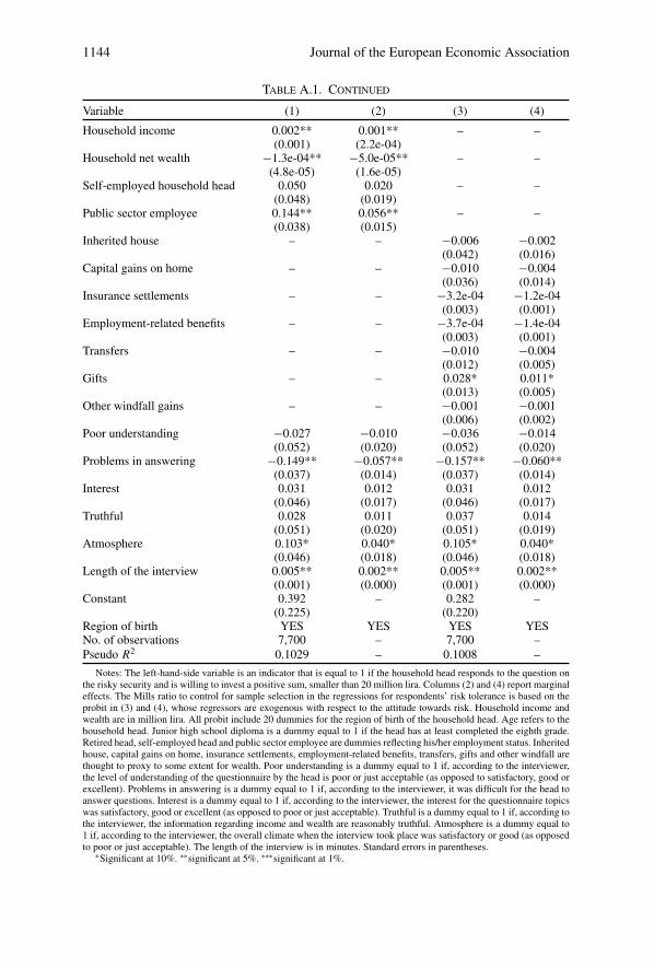
1144 Journal of the European Economic Association
Table A.1. Continued
Variable (1) (2) (3) (4)
Household income 0.002** 0.001** – –(0.001) (2.2e-04)
Household net wealth −1.3e-04** −5.0e-05** – –(4.8e-05) (1.6e-05)
Self-employed household head 0.050 0.020 – –(0.048) (0.019)
Public sector employee 0.144** 0.056** – –(0.038) (0.015)
Inherited house – – −0.006 −0.002(0.042) (0.016)
Capital gains on home – – −0.010 −0.004(0.036) (0.014)
Insurance settlements – – −3.2e-04 −1.2e-04(0.003) (0.001)
Employment-related benefits – – −3.7e-04 −1.4e-04(0.003) (0.001)
Transfers – – −0.010 −0.004(0.012) (0.005)
Gifts – – 0.028* 0.011*(0.013) (0.005)
Other windfall gains – – −0.001 −0.001(0.006) (0.002)
Poor understanding −0.027 −0.010 −0.036 −0.014(0.052) (0.020) (0.052) (0.020)
Problems in answering −0.149** −0.057** −0.157** −0.060**(0.037) (0.014) (0.037) (0.014)
Interest 0.031 0.012 0.031 0.012(0.046) (0.017) (0.046) (0.017)
Truthful 0.028 0.011 0.037 0.014(0.051) (0.020) (0.051) (0.019)
Atmosphere 0.103* 0.040* 0.105* 0.040*(0.046) (0.018) (0.046) (0.018)
Length of the interview 0.005** 0.002** 0.005** 0.002**(0.001) (0.000) (0.001) (0.000)
Constant 0.392 – 0.282 –(0.225) (0.220)
Region of birth YES YES YES YESNo. of observations 7,700 – 7,700 –Pseudo R2 0.1029 – 0.1008 –
Notes: The left-hand-side variable is an indicator that is equal to 1 if the household head responds to the question onthe risky security and is willing to invest a positive sum, smaller than 20 million lira. Columns (2) and (4) report marginaleffects. The Mills ratio to control for sample selection in the regressions for respondents’ risk tolerance is based on theprobit in (3) and (4), whose regressors are exogenous with respect to the attitude towards risk. Household income andwealth are in million lira. All probit include 20 dummies for the region of birth of the household head. Age refers to thehousehold head. Junior high school diploma is a dummy equal to 1 if the head has at least completed the eighth grade.Retired head, self-employed head and public sector employee are dummies reflecting his/her employment status. Inheritedhouse, capital gains on home, insurance settlements, employment-related benefits, transfers, gifts and other windfall arethought to proxy to some extent for wealth. Poor understanding is a dummy equal to 1 if, according to the interviewer,the level of understanding of the questionnaire by the head is poor or just acceptable (as opposed to satisfactory, good orexcellent). Problems in answering is a dummy equal to 1 if, according to the interviewer, it was difficult for the head toanswer questions. Interest is a dummy equal to 1 if, according to the interviewer, the interest for the questionnaire topicswas satisfactory, good or excellent (as opposed to poor or just acceptable). Truthful is a dummy equal to 1 if, according tothe interviewer, the information regarding income and wealth are reasonably truthful. Atmosphere is a dummy equal to1 if, according to the interviewer, the overall climate when the interview took place was satisfactory or good (as opposedto poor or just acceptable). The length of the interview is in minutes. Standard errors in parentheses.
∗Significant at 10%. ∗∗significant at 5%. ∗∗∗significant at 1%.

Guiso and Paiella Risk Aversion, Wealth, and Background Risk 1145
A.2. Definitions of the Variables
In the empirical analysis, all demographic variables (age, education, gender, num-ber of brothers and sisters, marital status, region of birth, occupation type, andsector) refer to the household head.
Consumption, net worth, and financial wealth. Consumption is the sum of theexpenditure on food, entertainment, education, clothing, medical expenses, hous-ing repairs and additions, and imputed rents. Net worth is the total of financialand real assets net of household debt. Financial wealth is given by the sum ofcash balances, checking accounts, savings accounts, postal deposits, governmentpaper, corporate bonds, mutual funds, and investment in fund units and stocks.Real assets include investment real estate, business wealth, primary residence,and the stock of durables.
Discouraged borrowers and rejected loan applicants. The following questionshave been asked in each wave of the survey since 1989: “During the year didyou or a member of the household think of applying for a loan or a mortgageto a bank or other financial intermediary, but then changed your mind on theexpectation that the application would be turned down?” Those answering Yesto this question are classified as discouraged borrowers. Those answering Yes tothe following questions are classified as rejected borrowers: “During the year didyou or a member of the household apply for a loan or a mortgage to a bank orother financial intermediary and have it turned down?”
Education of the household head’s father. This variable is originally coded as:no education (0); completed elementary school (5 years); completed junior highschool (8 years); completed high school (13 years); completed university (18years); graduate education (more than 20 years).
Education of the household head. This variable is originally coded exactly asthe previous (father) variable.
Income. Total household after-tax income, excluding asset income.
Indicators of background risk. The variance of shocks to per capita GDP in theprovince of residence is obtained from time-series data on per capita GDP at theprovince level from 1952 to 1992. For each province we regress the logarithm ofper capita GDP on a linear trend and compute the variance of the residuals fromthis regression. We then impute this variance to all households living in the sameprovince.

1146 Journal of the European Economic Association
Indicator of liquidity constraints. A dummy variable that allows for discour-aged borrowing and rejected loan applications and for low liquid assets or highindebtedness, which can prevent consumption smoothing in case of unexpectednegative income shocks.
Risk aversion. The Arrow–Pratt measure of absolute risk aversion; the riskattitude indicators are obtained from responses to a survey’s direct question con-cerning a hypothetical security. Each survey participant is offered a hypotheticalsecurity and is asked to report the maximum price that he would be willing topay in order to buy it. The wording of the security question and the methodologyimplemented to compute risk aversion are described in the text.
Year of birth of the household head’s father. This variable is used to define ten-year intervals starting from 1900. An additional interval is defined for those bornin or after 1950. We then construct six indicators: The first is set equal to 1 if thehousehold head’s father was born between 1900 and 1909, the second indicatoris set to 1 if he is born between 1910 and 1919, and so on.
Windfall gains measures. Six measures are used. The first is a dummy for homeownership as a result of gift or bequest. The second is the sum of the settlementsreceived related to life (excluding annuities), health, and casualty insurance. Thethird measure is the sum of severance payments, unemployment benefits, andredundancy allowance. The fourth is the sum of any additional financial aidfrom central or local governments, other public institutions, or charities. Thefifth consists of gifts/monetary contributions received from friends or family liv-ing outside the household dwelling. The last instrument is a measure of windfallgains (or losses) on housing constructed using time-series data on house prices atthe province level over the years 1965–1994. For homeowners, we compute thehouse price change since the year the house was acquired (or since 1965 if it wasacquired earlier). To non-homeowners, we assign the house price change sincethe year they started working (or since 1965). This can be justified on the groundsthat non-homeowners start saving to buy a home as soon as they start working.
A.3. Risk Aversion of the Indirect Utility Function
Let v(w) = Eu(w+ y) denote the indirect utility function. Taking a second-orderTaylor approximation of the right-hand side around the endowment w, we canapproximate the indirect utility by
v(w) � u(w) + u′′(w)σ 2/2.

Guiso and Paiella Risk Aversion, Wealth, and Background Risk 1147
Using the first and second derivatives of this expression, we can write the degreeof absolute risk aversion of v(·) as
Rv(w) = −v′′(w)
v′(w)� Ru(w)
(1 + PuTuσ
2/2
1 + PuRuσ 2/2
),
where Ru(w) = −(u′′/u′), Pu(w) = −(u′′′/u′′), and Tu(w) = −(uiv/u′′′)respectively denote the degrees of absolute risk aversion, absolute prudence, andabsolute temperance with respect to the utility function u(·). From the previouslydisplayed equation it is clear that Tu > Ru is a sufficient condition for (a zero-mean) background risk to make a prudent consumer more risk averse.
Let s denote the coefficient of variation of the consumer endowment (i.e.,s = σ/w) and let ru, pu, and tu denote the degrees of relative risk aversion,relative prudence, and relative temperance, respectively (obtained by multiplyingthe absolute degrees by w). We can then rewrite the absolute risk aversion of v(·) as
Rv(w) � Ru(w)
(1 + putus
2/2
1 + purus2/2
).
If the utility function is given by (8) in the text, then Ru = kw−β , ru = κw1−β ,pu = β + ru, and tu = β + pu. Substituting into the preceding expression forRv(w) and taking logs yields
log Rv � log κ − β log w + βpus2,
which shows that the parameter β of the utility function u(·) can be recoveredeven if there is background risk.
A.4. Implications of Measurement Error for the Estimation of β
Letlog T = − log α + β log c + ε
be the true relation, where T = f (Z). It can be shown that f (Z) is a convexfunction of Z. Instead of observing T we observe T = f (Z + u), where u is ameasurement error such that E(u) = 0 and E(c, u) = E(α, u) = 0. Hence, wecan estimate
log T = − log a + b log c + e.
Let log T = log f (Z) = h(Z) and log T = log(f (Z + u)) = h(Z + u).In general it is not clear whether the h(·) function is concave or convex. Taking

1148 Journal of the European Economic Association
a Taylor expansion of h(Z + u) around u = 0 and disregarding terms of orderhigher than the second, we obtain
log T ≈ h(Z) + h′(Z)u + 1
2h′′(Z)u2 = log T + h′(Z)u + 1
2h′′(Z)u2.
Using this expression, we can write our estimate of the elasticity of risk toleranceto the endowment as
b = (log c′ log c)−1(log c′ log T )
≈ β + (log c′ log c)−1 log c′h′(Z)u + (log c′ log c)−1 log c′h′′(Z)u2/2
andplim(β − β) ≈ plim(log c′ log c)−1 plim(log c′h′′(Z))σ 2
u /2.
If preferences are DARA then c and Z are positively correlated. Thus, the sign ofthe bias depends on the sign of h′′(Z). If h(·) is linear then there is no bias; if itis concave the bias is downward, and if it is convex the bias is upward. Becauseh′′(Z) = d2 log f (Z)/dz2, we can write h′′(Z) as
h′′(Z) = f (Z)−1[f ′′(Z) − f ′(Z)2
f (Z)
].
h′′(Z) is zero if and only if f ′′(Z) = f ′(Z)2/f (Z); this appears to be the casein our data, where h(·) turns out to be approximately linear.
References
Arrow, Kenneth (1965). Aspects of the Theory of Risk Bearing. Yrjö Jahnsson Lectures YrjöJahnsson Foundation, Helsinki.
Arrow, Kenneth (1970). Essays in the Theory of Risk-Bearing. North Holland.Barberis, Nicholas, Ming Huang, and Richard H. Thaler (2006). “Individual, Monetary Gam-
bles, and Stock Market Participation: A Case for Narrow Framing.” American EconomicReview, 96, 1069–1090.
Barsky, Robert, B., Thomas F. Juster, Miles S. Kimball, and Matthew D. Shapiro (1997).“Preference Parameters and Behavioral Heterogeneity: An Experimental Approach in theHealth and Retirement Study.” Quarterly Journal of Economics, 112, 537–580.
Benjamin, Daniel J., Sebastian A. Brown, and Jesse M. Shapiro (2006). “Who is ‘Behavioral’?Cognitive Ability and Anomalous Preferences.” Working Paper, University of Chicago.
Brandolini, Andrea, and Luigi Cannari (1994). “Methodological Appendix.” In “Saving and theAccumulation of Wealth,” edited by A. Ando, L. Guiso, and I. Visco. Cambridge UniversityPress.
Breeden, Douglas T. (1979). “An Intertemporal Asset Pricing Model with Stochastic Consump-tion and Investment Opportunities.” Journal of Financial Economics, 7, 265–296.
Carroll, Christopher (2000). “Portfolios of the Rich.” In “Household Portfolios,” edited by L.Guiso, M. Haliassos and T. Jappelli. MIT Press.

Guiso and Paiella Risk Aversion, Wealth, and Background Risk 1149
Carroll, Christopher, and Miles Kimball (1996). “On the Concavity of the ConsumptionFunction.” Econometrica, 64, 981–992.
Cascio, Elizabeth, and Ethan Lewis (2005). “Schooling and the AFQT: Evidence from SchoolEntry Laws.” NBER Working Paper No. 11113.
Eekhoudt Louis, and Miles Kimball (1992). “Background Risk, Prudence and the Demandfor Insurance.” In “Contributions to Insurance Economics,” edited by G. Dionne. KluwerAcademic Press.
Eekhoudt Louis, Christian Gollier, and Harris Schlesinger (1996). “Changes in BackgroundRisk and Risk Taking Behavior.” Econometrica, 64, 683–689.
Fuchs-Schündeln, Nicola, and Matthias Schündeln (2005). “Precautionary Savings and Self-Selection. Evidence from the German Reunification ‘Experiment?”’ Quarterly Journal ofEconomics, 120, 1085–1120.
Gollier Christian (2000). “What Does the Classical Theory Have to Say About PortfolioChoice?” In “Household Portfolios,” edited by L. Guiso, M. Haliassos, and T. Jappelli.MIT Press.
Gollier Christian (2001). “Wealth Inequality and Asset Pricing.” Review of Economic Studies,68, 181–203.
Gollier Christian, and John W. Pratt (1996). “Weak Proper Risk Aversion and the TemperingEffect of Background Risk.” Econometrica, 64, 1109–1123.
Gollier Christian, and Richard Zeckhauser (2002). “Horizon Length and Portfolio Risk.”Journal of Risk and Uncertainty, 24, 95–212.
Guiso, Luigi, and Tullio Jappelli (1998). “Background Uncertainty and the Demand forInsurance Against Insurable Risks.” Geneva Papers on Risk and Insurance Theory, 23,7–27.
Guiso, Luigi, and Tullio Jappelli (2000). “Household Portfolios in Italy.” In “HouseholdPortfolios,” edited by L. Guiso, M. Haliassos, and T. Jappelli. MIT Press.
Guiso, Luigi, and Tullio Jappelli (2006). “Information Acquisition and Portfolio Performance,”CEPR Working Paper No. 5901.
Guiso, Luigi, Tullio Jappelli, and Luigi Pistaferri (2002). “An Empirical Analysis of Earningsand Employment Risk.” Journal of Business and Economic Statistics, 20, 1–13.
Guiso, Luigi, Tullio Jappelli, and Daniele Terlizzese (1996). “Income Risk, BorrowingConstraints and Portfolio Choice.” American Economic Review, 86, 158–172.
Guiso, Luigi, and Monica Paiella (2006). “The Role of Risk Aversion in Predicting IndividualBehavior.” In “Insurance: Theoretical Analysis and Policy Implications,” edited by P. A.Chiappori and C. Gollier. MIT Press.
Heaton, John, and Deborah Lucas (2000). “Portfolio Choice in the Presence of BackgroundRisk.” Economic Journal, 110, 1–26.
Hennessy, David A., and Harvey E. Lapan (2006). “On the Nature of Certainty EquivalentFunctionals.” Journal of Mathematical Ecnomics, 43, 1–10.
Holt, Charles, and Susan K. Laury (2002). “Risk Aversion and Incentive Effects.” AmericanEconomic Review, 92, 1644–1655.
Hurd, Michael D. (2000). “Portfolio Holdings of the Elderly.” In “Household Portfolios,” editedby L. Guiso, M. Haliassos, and T. Jappelli. MIT Press.
Hurst, Erik, and Frank Stafford (2004). “Home Is Where Equity Is: Liquidity Constraints,Refinancing and Consumption.” Journal of Money, Credit and Banking, 36, 985–1014.
Kihlstrom, Richard E., David Romer, and Steve Williams (1981). “Risk Aversion with RandomInitial Wealth.” Econometrica, 49, 911–920.
Kimball, Miles (1993). “Standard Risk Aversion.” Econometrica, 61, 589–611.Kimball, Miles S., and Philippe Weil (2004). “Precautionary Saving and Consumption
Smoothing Across Time and Possibilities.” Working Paper, University of Michigan.Peress, Joel (2004). “Wealth, Information Acquisition and Portfolio Choice.” Review of
Financial Studies, 17, 879–914.

1150 Journal of the European Economic Association
Pratt, John (1964). “Risk Aversion in the Small and in the Large.” Econometrica, 32, 122–136.Pratt John W., and Richard Zeckhauser (1987). “Proper Risk Aversion.” Econometrica, 55,
143–154.Rabin, Matthew (2000). “Risk Aversion and Expected Utility Theory: A Calibration Theorem.”
Econometrica, 68, 1281–1292.Shane, Frederick (2005). “Cognitive Reflection and Decision Making.” Journal of Economic
Perspectives, 19, 25–42.Tiseno, Andrea (2002). “Using Wealth, Consumption and Shadow Prices to Identify Intertem-
poral Preferences.” Working Paper, University of Chicago.Tversky, Amos, and Daniel Kahneman (1992). “Advances in Prospect Theory: Cumulative
Representation of Uncertainty.” Journal of Risk and Uncertainty, 5, 297–323.Weil, Philippe (1992). “Equilibrium Asset Prices with Undiversifiable Labor Income Risk.”
Journal of Economic Dynamics and Control, 16, 769–790.