risk and asset allocation: value at risk, · pdf filerisk and asset allocation: value at risk,...
TRANSCRIPT
RISK AND ASSET ALLOCATION:
Value at Risk, Conditional-VaR and Copula Modelling
Dean Fantazzini
July 8-12th, 2007, Meielisalp, (Switzerland)

Overview of the Presentation
1st Introduction
1st International R/Rmetrics User and Developer Workshop 2
Overview of the Presentation
1st Introduction
2nd Risk Measures: VaR and C-VaR
1st International R/Rmetrics User and Developer Workshop 2-a
Overview of the Presentation
1st Introduction
2nd Risk Measures: VaR and C-VaR
3rd Advanced Multivariate Modelling: The Theory of Copulas
1st International R/Rmetrics User and Developer Workshop 2-b
Overview of the Presentation
1st Introduction
2nd Risk Measures: VaR and C-VaR
3rd Advanced Multivariate Modelling: The Theory of Copulas
4th Empirical Applications: Market Risk Management for Bivariate
Portfolios
1st International R/Rmetrics User and Developer Workshop 2-c

Overview of the Presentation
1st Introduction
2nd Risk Measures: VaR and C-VaR
3rd Advanced Multivariate Modelling: The Theory of Copulas
4th Empirical Applications: Market Risk Management for Bivariate
Portfolios
5th Empirical Applications: Market Risk Management for
Multivariate Portfolios (Dynamic Grouped-T and T-copulas)
1st International R/Rmetrics User and Developer Workshop 2-d

Overview of the Presentation
1st Introduction
2nd Risk Measures: VaR and C-VaR
3rd Advanced Multivariate Modelling: The Theory of Copulas
4th Empirical Applications: Market Risk Management for Bivariate
Portfolios
5th Empirical Applications: Market Risk Management for
Multivariate Portfolios (Dynamic Grouped-T and T-copulas)
6th Empirical Applications: C-VaR and VaR for Portfolio
Management
1st International R/Rmetrics User and Developer Workshop 2-e
Introduction
In the Mean-Variance model, the risk of a portfolio measured by the
variance takes into account the covariances among the returns of all
investments.
However, this approach is appropriate when dealing with multivariate
Elliptic distributions only, like the multivariate Normal or the multivariate
Student’s T joint distribution.
→ Only if the joint distribution function is elliptical the Markowitz
Mean-Variance approach can give efficient portfolios.
Therefore, more general risk measures have been proposed: the Value at
Risk and (more recently) the Conditional Value at Risk.
1st International R/Rmetrics User and Developer Workshop 3
Introduction
The increasing complexity of financial markets has pointed out the need
for advanced dependence modelling in finance. Why?
• Multivariate models with more flexibility than the multivariate normal
distribution are needed;
• When constructing a model for risk management, the study of both
marginals and the dependence structure is crucial for the analysis. A
wrong choice may lead to severe underestimation of financial risks.
Recent developments in financial studies have tried to tackle these issues
by using the theory of Copulas: see Cherubini et al. (2004) for a general
review of copula methods in finance.
1st International R/Rmetrics User and Developer Workshop 4
Coherent Risk Measures
Artzner, Delbaen, Eber and Heath (1999) examined the issue of setting out
the axioms that a coherent risk measure ought to satisfy. They then looked
for measures that satisfy these properties.
If X and Y are the random variables representing the future values of two
risky investments, a risk measure ρ(·) is said to be coherent if it satisfies
the following properties:
1. Sub-additivity : ρ(X + Y ) ≤ ρ(X) + ρ(Y ) (diversification effect).
2. Monotonicity : ρ(X) ≤ ρ(Y ) whenever X ≤ Y (the bigger the loss the
bigger the risk).
3. Homogeneity : ρ(λX) = λρ(X) for λ > 0 (the risk scales in proportion
to a scaled loss).
4. Translation invariance: ρ(X + rn) = ρ(X) − n (reduction of risk by
investing in the risk-free payoff r).
1st International R/Rmetrics User and Developer Workshop 5
Risk Measures: Value at Risk
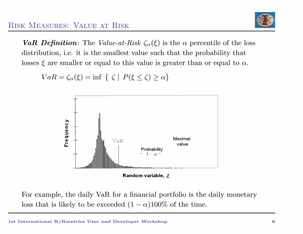
VaR Definition : The Value-at-Risk ζα(ξ) is the α percentile of the loss
distribution, i.e. it is the smallest value such that the probability that
losses ξ are smaller or equal to this value is greater than or equal to α.
V aR = ζα(ξ) = inf { ζ | P (ξ ≤ ζ) ≥ α}
For example, the daily VaR for a financial portfolio is the daily monetary
loss that is likely to be exceeded (1 − α)100% of the time.
1st International R/Rmetrics User and Developer Workshop 6
Risk Measures: Value at Risk
• VaR Properties:
• Simple convenient representation of risks (one number);
• Measures downside risk (compared to variance which is impacted by
high returns);
• applicable to nonlinear instruments, such as options, with non-
symmetric (non-normal) loss distributions;
• Does not measure losses exceeding VaR (e.g., excluding or doubling of
big losses in November 1987 may not impact VaR historical estimates)
• Reduction of VaR may lead to stretch of tail exceeding VaR (Yamai
and Yoshiba, 2002)
• Since VaR does not take into account risks exceeding VaR, it may
provide conflicting results at different confidence levels;
• Non-sub-additive and non-convex (portfolio diversification may
increase the risk - Difficult to optimize for non-normal distribution);
1st International R/Rmetrics User and Developer Workshop 7
Risk Measures: Value at Risk
Example of VaR Non-sub-additivity :
Suppose one has a portfolio that is made up by a Trader A and Trader B. Trader
A has a portfolio that consists of a put that is out of money, and has one day to
expiry. Trader B has a portfolio that consists of a call that is also far out of the
money and also one day to expiry. Using any historical VaR approach, say we
find that each option has a probability of 4 % of ending up in the money.
Trader A and B each have a portfolio that has a 96 % chance of not losing any
money, so each has a 95% VaR of zero. However, the combined portfolio has only
a 92% chance of not losing any money, so its VaR is non-trivial.
7→ Negative diversification benefit if VaR is used to measure the diversification
benefit!
1st International R/Rmetrics User and Developer Workshop 8
Risk Measures: Conditional Value at Risk
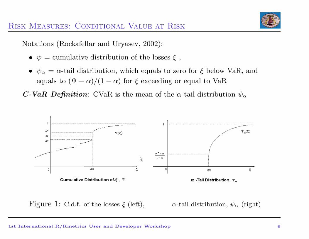
Notations (Rockafellar and Uryasev, 2002):
• ψ = cumulative distribution of the losses ξ ,
• ψα = α-tail distribution, which equals to zero for ξ below VaR, and
equals to (Ψ − α)/(1 − α) for ξ exceeding or equal to VaR
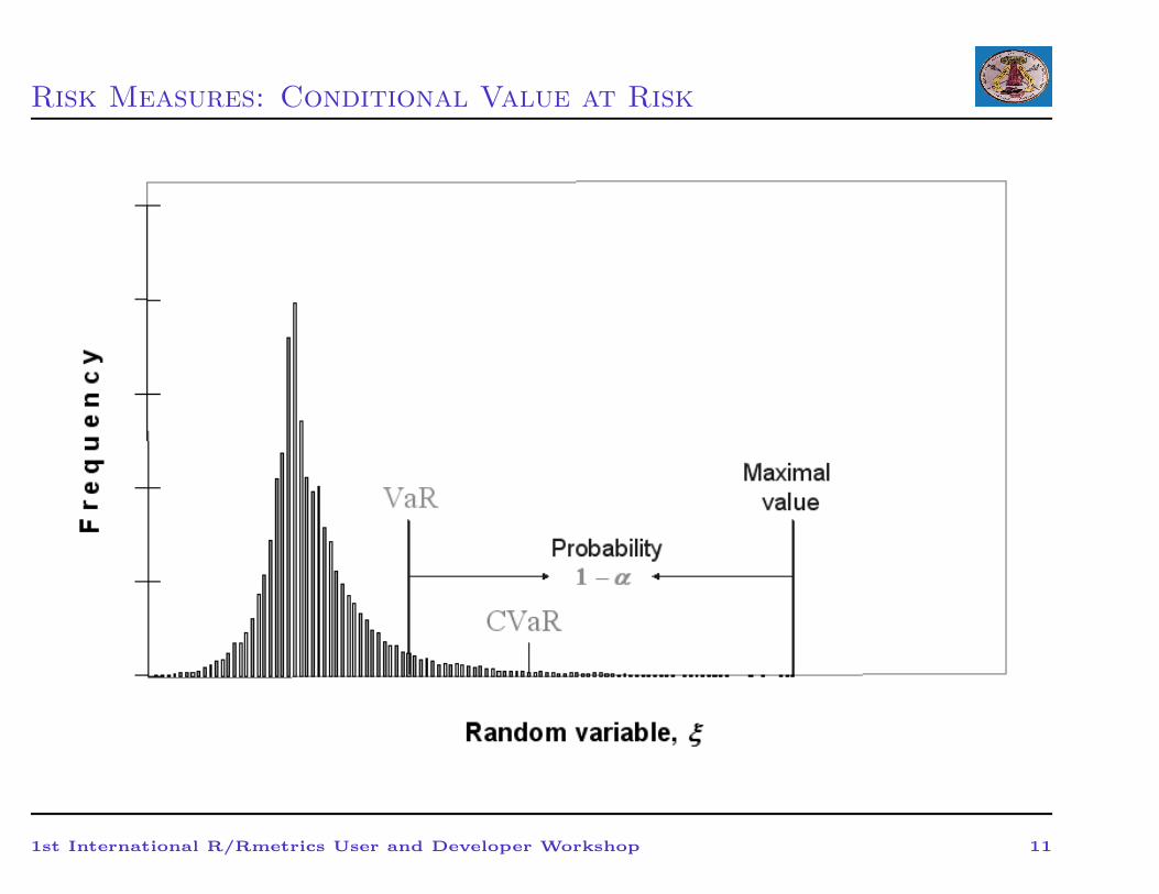
C-VaR Definition : CVaR is the mean of the α-tail distribution ψα
Figure 1: C.d.f. of the losses ξ (left), α-tail distribution, ψα (right)
1st International R/Rmetrics User and Developer Workshop 9
Risk Measures: Conditional Value at Risk
Notations:
• CVaR+ (“upper CVaR”) = expected value of losses ξ strictly
exceeding VaR (also called Mean Excess Loss and Expected Shortfall)
• CVaR− (“lower CVaR”) = expected value of losses ξ weakly exceeding
VaR, i.e., value of ξ which are equal to or exceed VaR (also called Tail
VaR)
• Ψ(VaR) = probability that ξ does not exceed VaR or equal to VaR
Property: CVaR is a weighted average of VaR and CVaR+
CV aRα(ξ) = λVaR + (1 − λ)CVaR+α (ξ)
λ = (Ψ(ζα) − α) (1 − α), 0 ≤ λ ≤ 1
1st International R/Rmetrics User and Developer Workshop 10
Risk Measures: Conditional Value at Risk
1st International R/Rmetrics User and Developer Workshop 11
Risk Measures: Conditional Value at Risk
• C-VaR Properties:
• Simple convenient representation of risks (one number);
• Measures downside risk applicable to non-symmetric loss distributions
CVaR accounts for risks beyond VaR (more conservative than VaR);
• CVaR is convex with respect to control variables;
• VaR ≤ CVaR− ≤ CVaR ≤ CVaR+
• CVaR is continuous with respect to confidence level alpha, consistent
at different confidence levels compared to VaR;
• Consistency with mean-variance approach: for normal loss
distributions optimal variance and CVaR portfolios coincide;
• Easy to control/optimize for non-normal distributions; linear
programming (LP): can be used for optimization of very large
problems.
1st International R/Rmetrics User and Developer Workshop 12
Risk Measures: Conditional Value at Risk
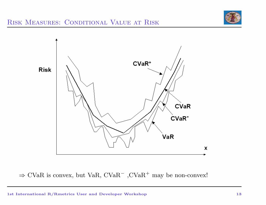
⇒ CVaR is convex, but VaR, CVaR− ,CVaR+ may be non-convex!
1st International R/Rmetrics User and Developer Workshop 13
Risk Measures: Some Examples
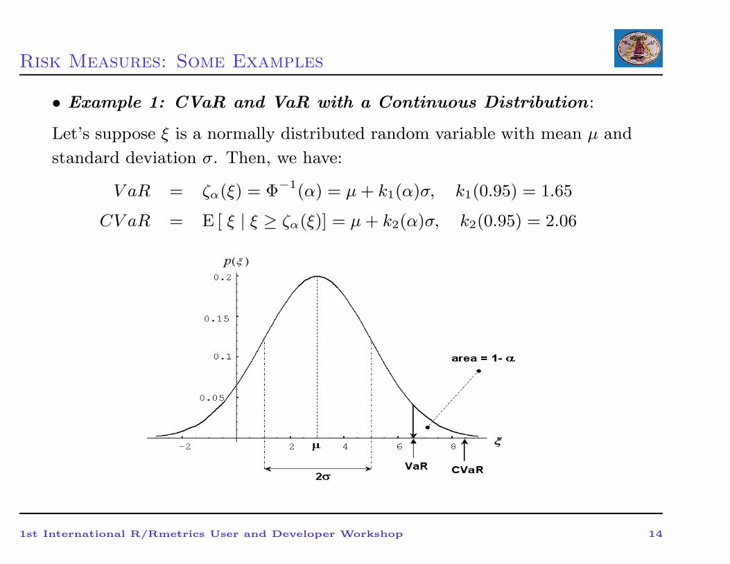
• Example 1: CVaR and VaR with a Continuous Distribution :
Let’s suppose ξ is a normally distributed random variable with mean µ and
standard deviation σ. Then, we have:
V aR = ζα(ξ) = Φ−1(α) = µ+ k1(α)σ, k1(0.95) = 1.65
CV aR = E [ ξ | ξ ≥ ζα(ξ)] = µ+ k2(α)σ, k2(0.95) = 2.06
1st International R/Rmetrics User and Developer Workshop 14
Risk Measures: Some Examples
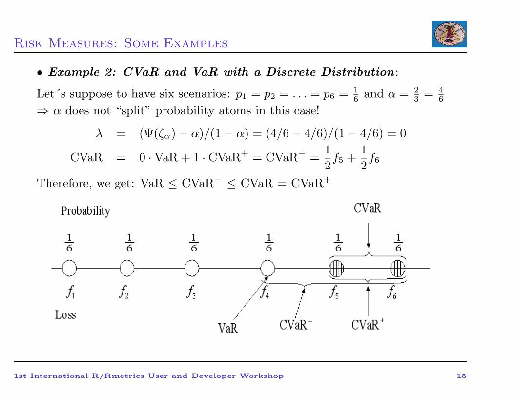
• Example 2: CVaR and VaR with a Discrete Distribution :
Let´s suppose to have six scenarios: p1 = p2 = . . . = p6 = 16
and α = 23
= 46
⇒ α does not “split” probability atoms in this case!
λ = (Ψ(ζα) − α)/(1 − α) = (4/6 − 4/6)/(1 − 4/6) = 0
CVaR = 0 · VaR + 1 · CVaR+ = CVaR+ =1
2f5 +
1
2f6
Therefore, we get: VaR ≤ CVaR− ≤ CVaR = CVaR+
1st International R/Rmetrics User and Developer Workshop 15
Risk Measures: Some Examples
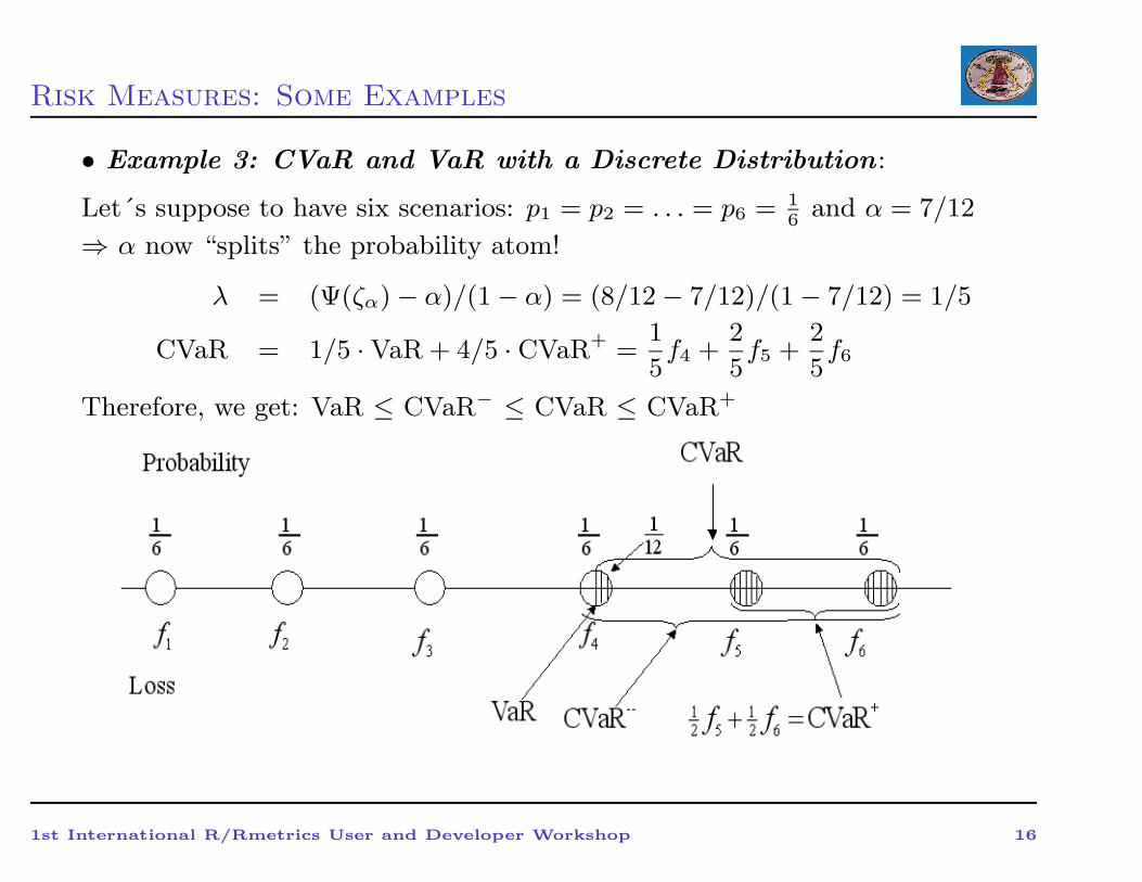
• Example 3: CVaR and VaR with a Discrete Distribution :
Let´s suppose to have six scenarios: p1 = p2 = . . . = p6 = 16
and α = 7/12
⇒ α now “splits” the probability atom!
λ = (Ψ(ζα) − α)/(1 − α) = (8/12 − 7/12)/(1 − 7/12) = 1/5
CVaR = 1/5 · VaR + 4/5 · CVaR+ =1
5f4 +
2
5f5 +
2
5f6
Therefore, we get: VaR ≤ CVaR− ≤ CVaR ≤ CVaR+
1st International R/Rmetrics User and Developer Workshop 16
Advanced Multivariate Modelling: The Theory of Copulas
→ A copula is a multivariate distribution function H of random variables
X1 . . . Xn with standard uniform marginal distributions F1, . . . , Fn,
defined on the unit n-cube [0,1]n with the following properties:
1. The range of C (u1, u2, ..., un) is the unit interval [0,1];
2. C (u1, u2, ..., un) = 0 if any ui = 0, for i = 1, 2, ..., n.
3. C (1, ..., 1, ui, 1, ..., 1) = ui , for all ui ∈ [0, 1]
The previous three conditions provides the lower bound on the distribution
function and ensures that the marginal distributions are uniform.
The Sklar’s theorem justifies the role of copulas as dependence functions...
1st International R/Rmetrics User and Developer Workshop 17
Advanced Multivariate Modelling: The Theory of Copulas
(Sklar’s theorem): Let H denote a n-dimensional distribution function
with margins F1. . .Fn . Then there exists a n-copula C such that for all
real (x1,. . . , xn)
H(x1, . . . , xn) = C(F1(x1), . . . , Fn(xn)) (1)
If all the margins are continuous, then the copula is unique. Conversely, if
C is a copula and F1, . . . Fn are distribution functions, then the function H
defined in (1) is a joint distribution function with margins F1, . . . Fn.
→ A copula is a function that links univariate marginal distributions of
two or more variables to their multivariate distribution.
→ F1 and Fn need not to be identical or even to belong to the same
distribution family.
1st International R/Rmetrics User and Developer Workshop 18
Advanced Multivariate Modelling: The Theory of Copulas
Main consequences:
• For continuous multivariate distributions, the univariate margins and
the multivariate dependence can be separated;
• Copula is invariant under strictly increasing and continuous
transformations: no matter whether we work with price series or with
log-prices.
Example. Independent copula: C(u, v) = u · v
What is the probability that both returns in market A and B are in their
lowest 10th percentiles?
C(0.1; 0.1) = 0.1 · 0.1 = 0.01
1st International R/Rmetrics User and Developer Workshop 19
Advanced Multivariate Modelling: The Theory of Copulas
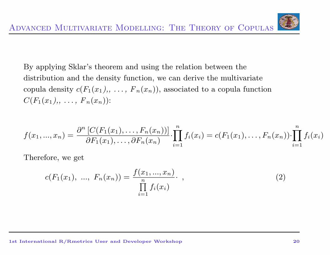
By applying Sklar’s theorem and using the relation between the
distribution and the density function, we can derive the multivariate
copula density c(F1(x1),, . . . , Fn(xn)), associated to a copula function
C(F1(x1),, . . . , Fn(xn)):
f(x1, ..., xn) =∂n [C(F1(x1), . . . , Fn(xn))]
∂F1(x1), . . . , ∂Fn(xn)·
n∏
i=1
fi(xi) = c(F1(x1), . . . , Fn(xn))·n∏
i=1
fi(xi)
Therefore, we get
c(F1(x1), ..., Fn(xn)) =f(x1, ..., xn)
n∏
i=1
fi(xi)· , (2)
1st International R/Rmetrics User and Developer Workshop 20
Advanced Multivariate Modelling: The Theory of Copulas
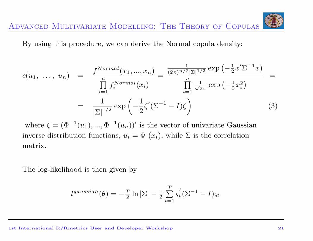
By using this procedure, we can derive the Normal copula density:
c(u1, . . . , un) =fNormal(x1, ..., xn)
n∏
i=1
fNormali (xi)
=
1
(2π)n/2|Σ|1/2 exp(
− 12x′Σ−1x
)
n∏
i=1
1√2π
exp(
− 12x2
i
)
=
=1
|Σ|1/2exp
(
−1
2ζ′(Σ−1 − I)ζ
)
(3)
where ζ = (Φ−1(u1), ...,Φ−1(un))′ is the vector of univariate Gaussian
inverse distribution functions, ui = Φ (xi), while Σ is the correlation
matrix.
The log-likelihood is then given by
lgaussian(θ) = −T2
ln |Σ| − 12
T∑
t=1
ς′
t(Σ−1 − I)ςt
1st International R/Rmetrics User and Developer Workshop 21
Advanced Multivariate Modelling: The Theory of Copulas
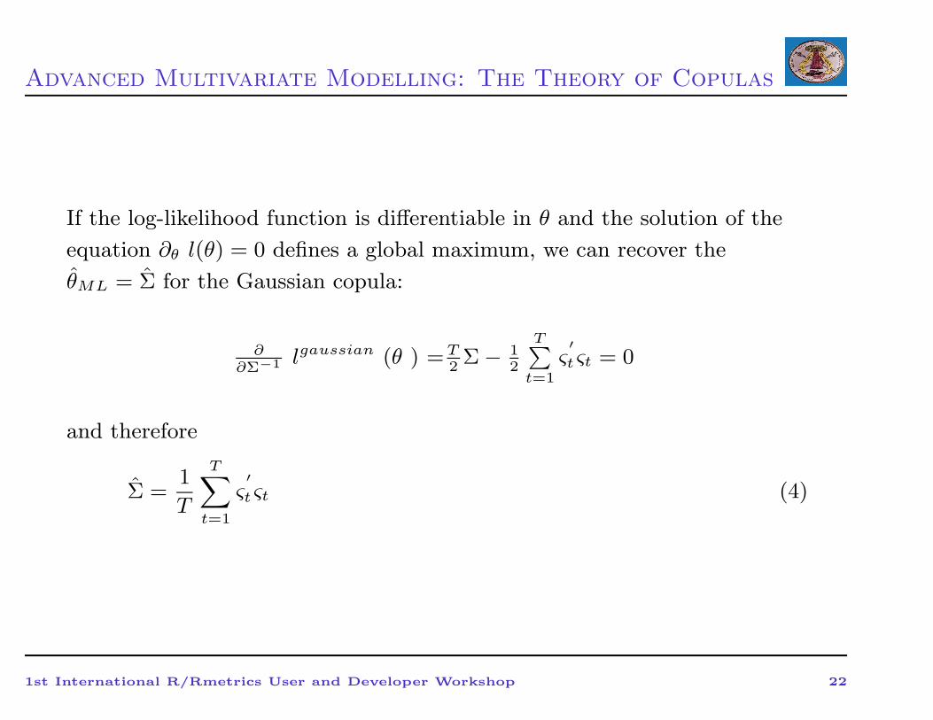
If the log-likelihood function is differentiable in θ and the solution of the
equation ∂θ l(θ) = 0 defines a global maximum, we can recover the
θML = Σ for the Gaussian copula:
∂∂Σ−1 lgaussian (θ ) =T
2Σ − 1
2
T∑
t=1
ς′
t ςt = 0
and therefore
Σ =1
T
T∑
t=1
ς′
t ςt (4)
1st International R/Rmetrics User and Developer Workshop 22
Advanced Multivariate Modelling: The Theory of Copulas
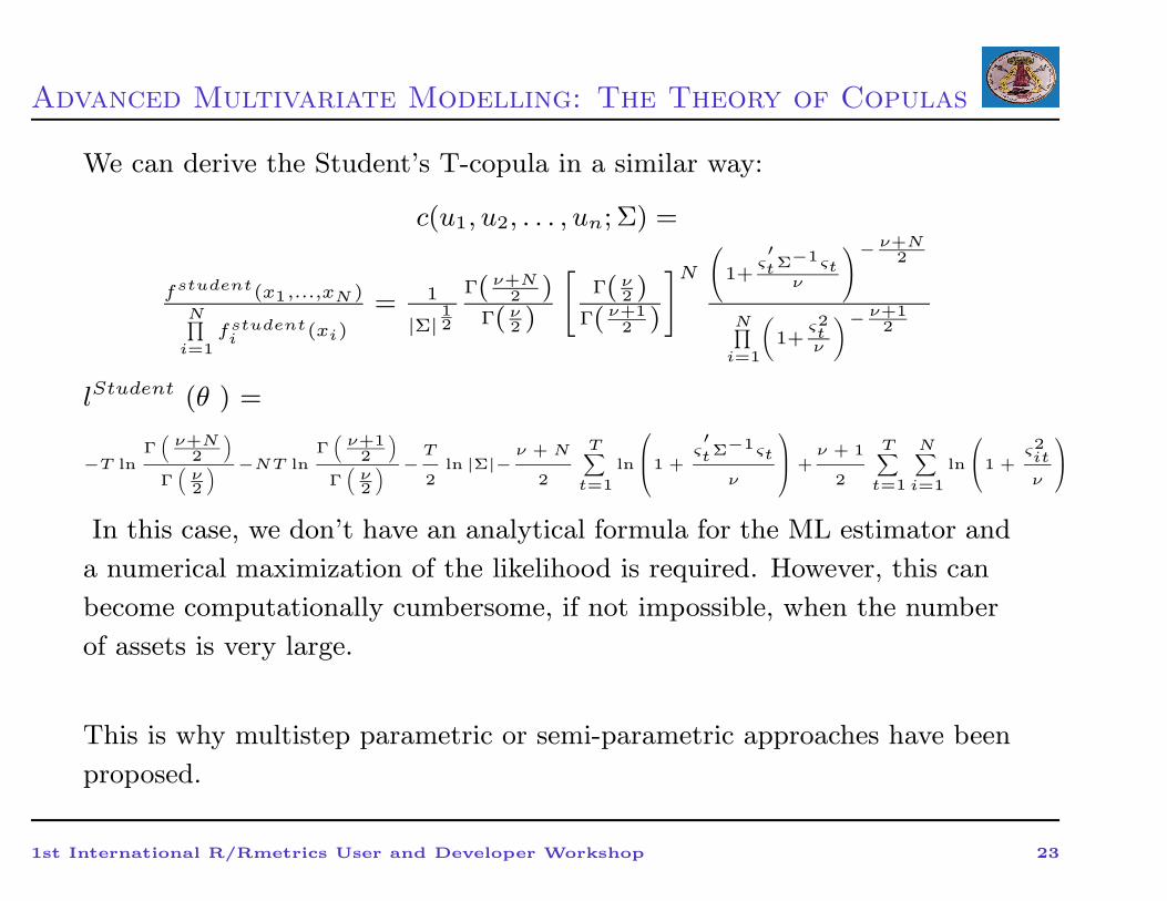
We can derive the Student’s T-copula in a similar way:
c(u1, u2, . . . , un; Σ) =
fstudent(x1,...,xN )N∏
i=1fstudent
i (xi)
= 1
|Σ|12
Γ( ν+N2 )
Γ( ν2 )
[
Γ( ν2 )
Γ( ν+12 )
]N
(
1+ς′tΣ−1ςt
ν
)− ν+N2
N∏
i=1
(
1+ς2tν
)− ν+12
lStudent (θ ) =
−T lnΓ(
ν+N2
)
Γ(
ν2
) −NT lnΓ(
ν+12
)
Γ(
ν2
) −T
2ln |Σ|−
ν + N
2
T∑
t=1
ln
1 +
ς′tΣ−1ςt
ν
+
ν + 1
2
T∑
t=1
N∑
i=1
ln
1 +ς2it
ν
In this case, we don’t have an analytical formula for the ML estimator and
a numerical maximization of the likelihood is required. However, this can
become computationally cumbersome, if not impossible, when the number
of assets is very large.
This is why multistep parametric or semi-parametric approaches have been
proposed.
1st International R/Rmetrics User and Developer Workshop 23
Empirical Applications: Market Risk Management:
Overview of the Presentation
• Aim: Build flexible multivariate distribution, without the
constraints of the traditional joint normal distribution.
• Aim 2 : Evaluate what are the main determinants when doing
VaR forecasts for a portfolio of assets.
• Contribution: Copulae capture those properties of the joint
distribution which are invariant under strictly increasing
transformation and do not depend on marginals and allow for
time dependency
• Benefit : More precise portfolio Value at Risk estimates
1st International R/Rmetrics User and Developer Workshop 24
Empirical Applications: Market Risk Management:
Copula: Definitions and Estimation method
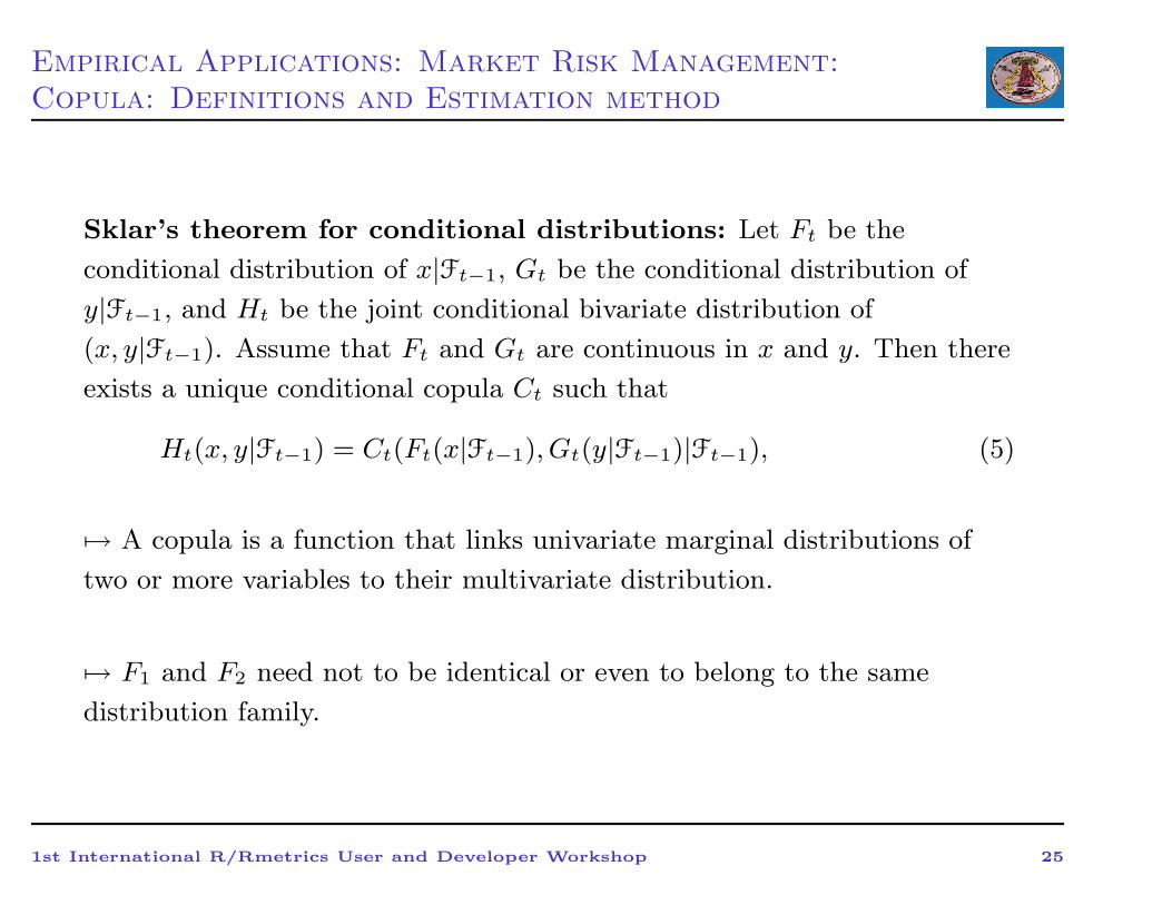
Sklar’s theorem for conditional distributions: Let Ft be the
conditional distribution of x|Ft−1, Gt be the conditional distribution of
y|Ft−1, and Ht be the joint conditional bivariate distribution of
(x, y|Ft−1). Assume that Ft and Gt are continuous in x and y. Then there
exists a unique conditional copula Ct such that
Ht(x, y|Ft−1) = Ct(Ft(x|Ft−1), Gt(y|Ft−1)|Ft−1), (5)
7→ A copula is a function that links univariate marginal distributions of
two or more variables to their multivariate distribution.
7→ F1 and F2 need not to be identical or even to belong to the same
distribution family.
1st International R/Rmetrics User and Developer Workshop 25
Empirical Applications: Market Risk Management:
Copula: Definitions and Estimation method
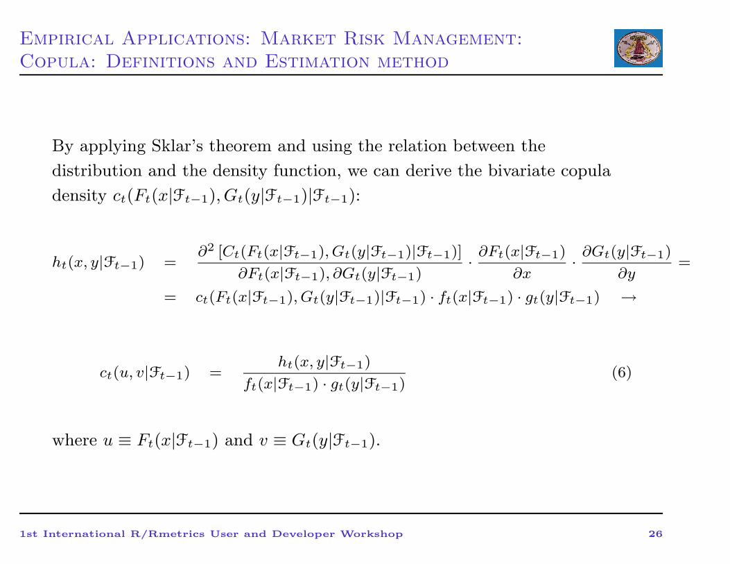
By applying Sklar’s theorem and using the relation between the
distribution and the density function, we can derive the bivariate copula
density ct(Ft(x|Ft−1), Gt(y|Ft−1)|Ft−1):
ht(x, y|Ft−1) =∂2 [Ct(Ft(x|Ft−1), Gt(y|Ft−1)|Ft−1)]
∂Ft(x|Ft−1), ∂Gt(y|Ft−1)· ∂Ft(x|Ft−1)
∂x· ∂Gt(y|Ft−1)
∂y=
= ct(Ft(x|Ft−1), Gt(y|Ft−1)|Ft−1) · ft(x|Ft−1) · gt(y|Ft−1) →
ct(u, v|Ft−1) =ht(x, y|Ft−1)
ft(x|Ft−1) · gt(y|Ft−1)(6)
where u ≡ Ft(x|Ft−1) and v ≡ Gt(y|Ft−1).
1st International R/Rmetrics User and Developer Workshop 26
Empirical Applications: Market Risk Management:
Copula: Definitions and Estimation method
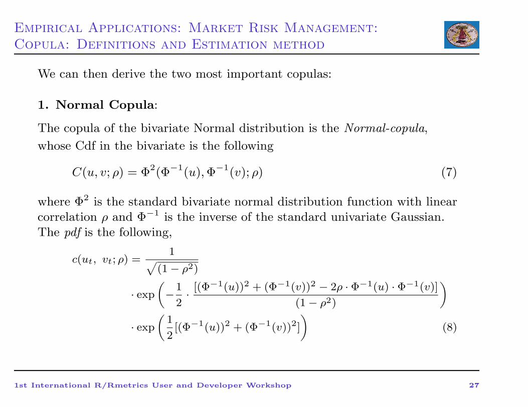
We can then derive the two most important copulas:
1. Normal Copula:
The copula of the bivariate Normal distribution is the Normal-copula,
whose Cdf in the bivariate is the following
C(u, v; ρ) = Φ2(Φ−1(u),Φ−1(v); ρ) (7)
where Φ2 is the standard bivariate normal distribution function with linearcorrelation ρ and Φ−1 is the inverse of the standard univariate Gaussian.The pdf is the following,
c(ut, vt; ρ) =1
√
(1 − ρ2)
· exp
(
−1
2· [(Φ−1(u))2 + (Φ−1(v))2 − 2ρ · Φ−1(u) · Φ−1(v)]
(1 − ρ2)
)
· exp
(
1
2[(Φ−1(u))2 + (Φ−1(v))2]
)
(8)
1st International R/Rmetrics User and Developer Workshop 27
Empirical Applications: Market Risk Management:
Copula: Definitions and Estimation method
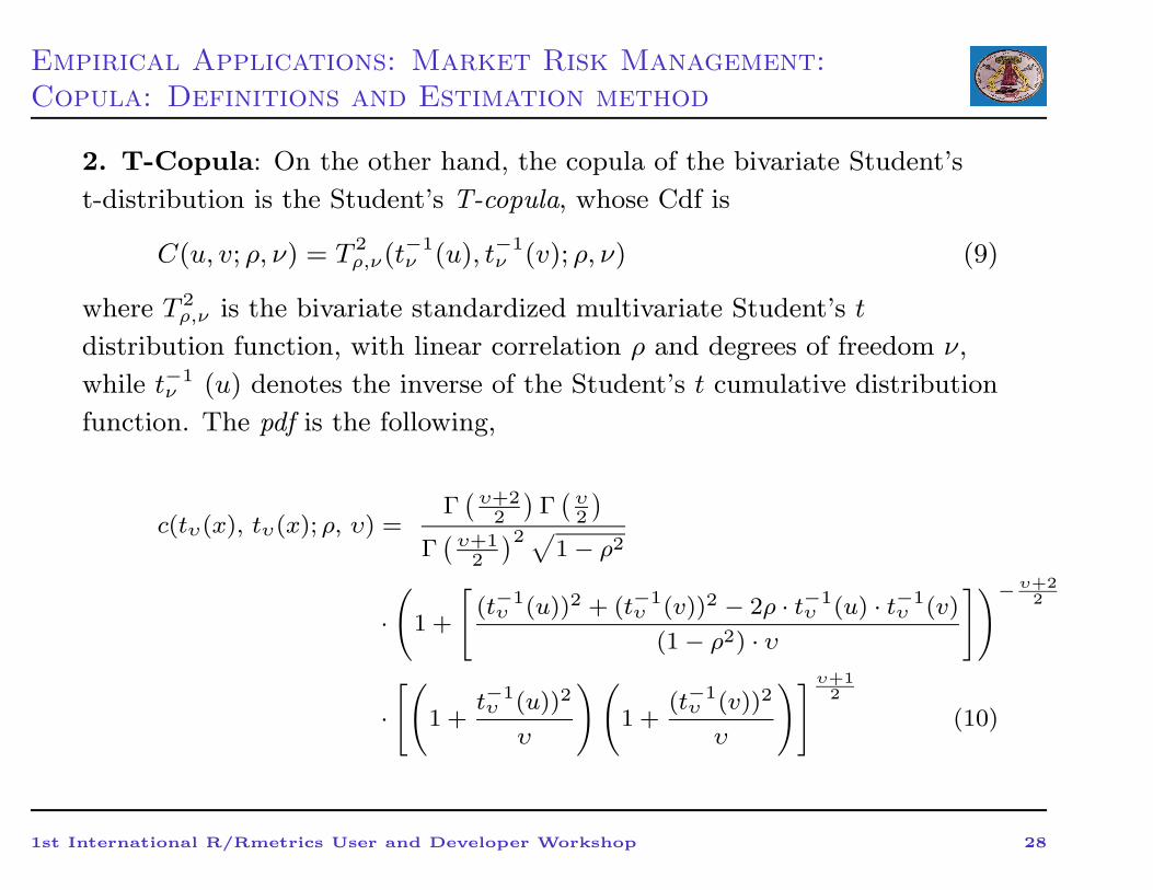
2. T-Copula: On the other hand, the copula of the bivariate Student’s
t-distribution is the Student’s T-copula, whose Cdf is
C(u, v; ρ, ν) = T 2ρ,ν(t−1
ν (u), t−1ν (v); ρ, ν) (9)
where T 2ρ,ν is the bivariate standardized multivariate Student’s t
distribution function, with linear correlation ρ and degrees of freedom ν,
while t−1ν (u) denotes the inverse of the Student’s t cumulative distribution
function. The pdf is the following,
c(tυ(x), tυ(x); ρ, υ) =Γ(
υ+22
)
Γ(
υ2
)
Γ(
υ+12
)2√1 − ρ2
·(
1 +
[
(t−1υ (u))2 + (t−1
υ (v))2 − 2ρ · t−1υ (u) · t−1
υ (v)
(1 − ρ2) · υ
])− υ+22
·[(
1 +t−1υ (u))2
υ
)(
1 +(t−1
υ (v))2
υ
)]υ+12
(10)
1st International R/Rmetrics User and Developer Workshop 28
Empirical Applications: Market Risk Management:
Copula: Definitions and Estimation method
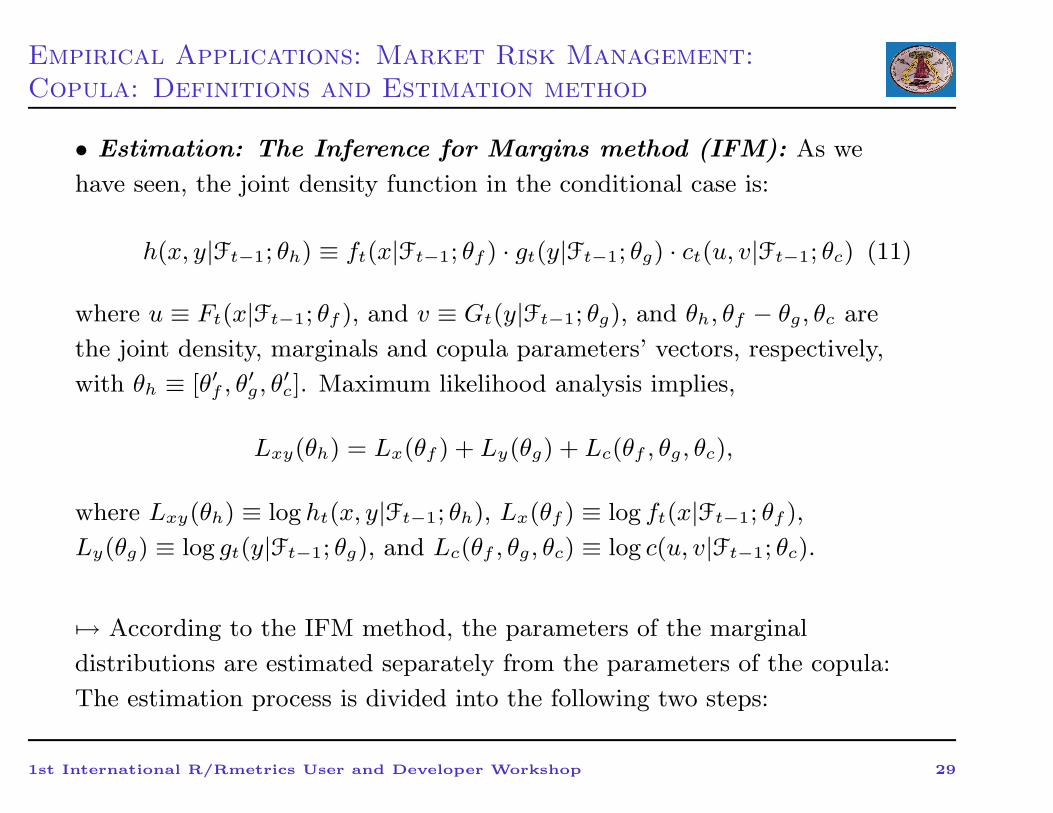
• Estimation: The Inference for Margins method (IFM): As we
have seen, the joint density function in the conditional case is:
h(x, y|Ft−1; θh) ≡ ft(x|Ft−1; θf ) · gt(y|Ft−1; θg) · ct(u, v|Ft−1; θc) (11)
where u ≡ Ft(x|Ft−1; θf ), and v ≡ Gt(y|Ft−1; θg), and θh, θf − θg, θc are
the joint density, marginals and copula parameters’ vectors, respectively,
with θh ≡ [θ′f , θ′g, θ
′c]. Maximum likelihood analysis implies,
Lxy(θh) = Lx(θf ) + Ly(θg) + Lc(θf , θg, θc),
where Lxy(θh) ≡ log ht(x, y|Ft−1; θh), Lx(θf ) ≡ log ft(x|Ft−1; θf ),
Ly(θg) ≡ log gt(y|Ft−1; θg), and Lc(θf , θg, θc) ≡ log c(u, v|Ft−1; θc).
7→ According to the IFM method, the parameters of the marginal
distributions are estimated separately from the parameters of the copula:
The estimation process is divided into the following two steps:
1st International R/Rmetrics User and Developer Workshop 29
Empirical Applications: Market Risk Management:
Copula: Definitions and Estimation method
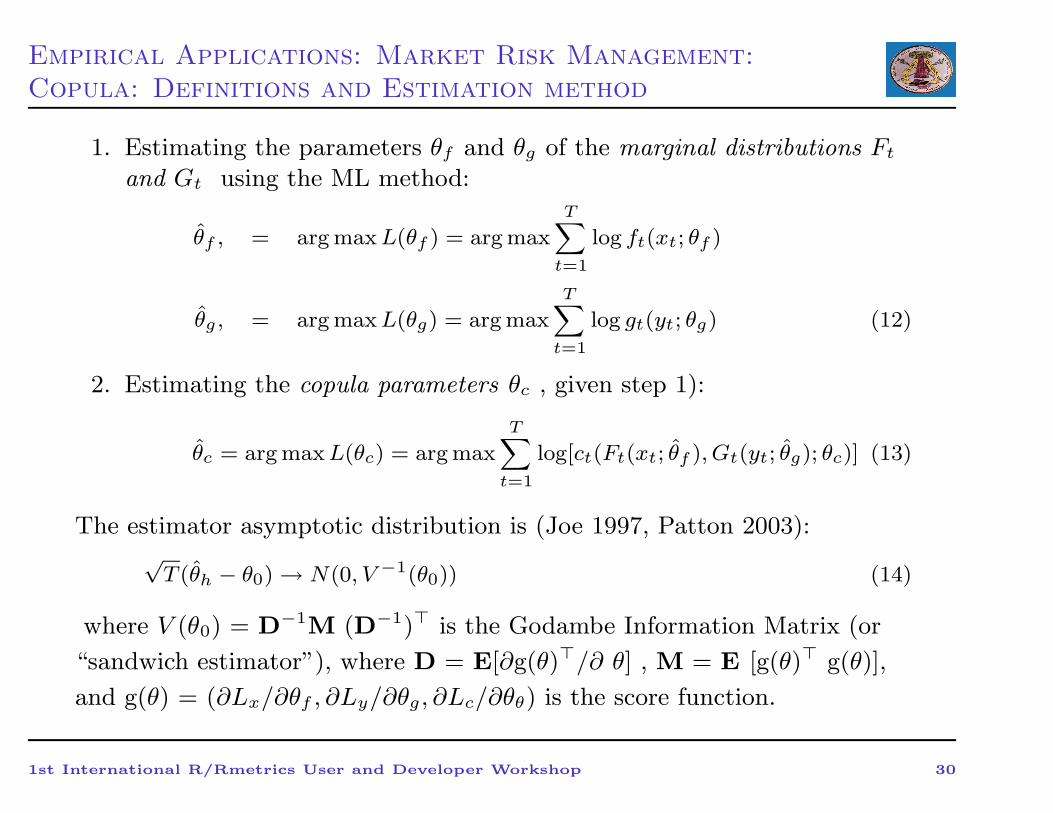
1. Estimating the parameters θf and θg of the marginal distributions Ft
and Gt using the ML method:
θf , = arg maxL(θf ) = arg max
T∑
t=1
log ft(xt; θf )
θg , = arg maxL(θg) = arg max
T∑
t=1
log gt(yt; θg) (12)
2. Estimating the copula parameters θc , given step 1):
θc = arg maxL(θc) = arg max
T∑
t=1
log[ct(Ft(xt; θf ), Gt(yt; θg); θc)] (13)
The estimator asymptotic distribution is (Joe 1997, Patton 2003):√T (θh − θ0) → N(0, V −1(θ0)) (14)
where V (θ0) = D−1M (D−1)⊤ is the Godambe Information Matrix (or
“sandwich estimator”), where D = E[∂g(θ)⊤/∂ θ] , M = E [g(θ)⊤ g(θ)],
and g(θ) = (∂Lx/∂θf , ∂Ly/∂θg, ∂Lc/∂θθ) is the score function.
1st International R/Rmetrics User and Developer Workshop 30
Empirical Applications: Market Risk Management:
Copula: Definitions and Estimation method
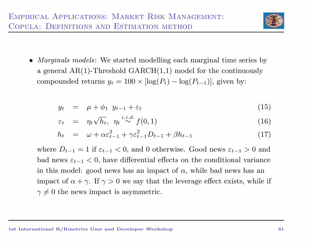
• Marginals models: We started modelling each marginal time series by
a general AR(1)-Threshold GARCH(1,1) model for the continuously
compounded returns yt = 100 × [log(Pt) − log(Pt−1)], given by:
yt = µ+ φ1 yt−1 + εt (15)
εt = ηt
√ht, ηt
i.i.d.∼ f(0, 1) (16)
ht = ω + αε2t−1 + γε2t−1Dt−1 + βht−1 (17)
where Dt−1 = 1 if εt−1 < 0, and 0 otherwise. Good news εt−1 > 0 and
bad news εt−1 < 0, have differential effects on the conditional variance
in this model: good news has an impact of α, while bad news has an
impact of α+ γ. If γ > 0 we say that the leverage effect exists, while if
γ 6= 0 the news impact is asymmetric.
1st International R/Rmetrics User and Developer Workshop 31
Empirical Applications: Market Risk Management:
Copula: Definitions and Estimation method
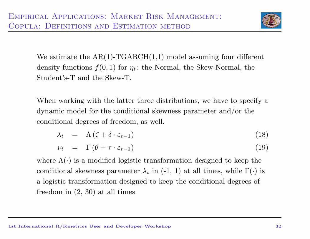
We estimate the AR(1)-TGARCH(1,1) model assuming four different
density functions f(0, 1) for ηt: the Normal, the Skew-Normal, the
Student’s-T and the Skew-T.
When working with the latter three distributions, we have to specify a
dynamic model for the conditional skewness parameter and/or the
conditional degrees of freedom, as well.
λt = Λ (ζ + δ · εt−1) (18)
νt = Γ (θ + τ · εt−1) (19)
where Λ(·) is a modified logistic transformation designed to keep the
conditional skewness parameter λt in (-1, 1) at all times, while Γ(·) is
a logistic transformation designed to keep the conditional degrees of
freedom in (2, 30) at all times
1st International R/Rmetrics User and Developer Workshop 32
Empirical Applications: Market Risk Management:
Copula: Definitions and Estimation method
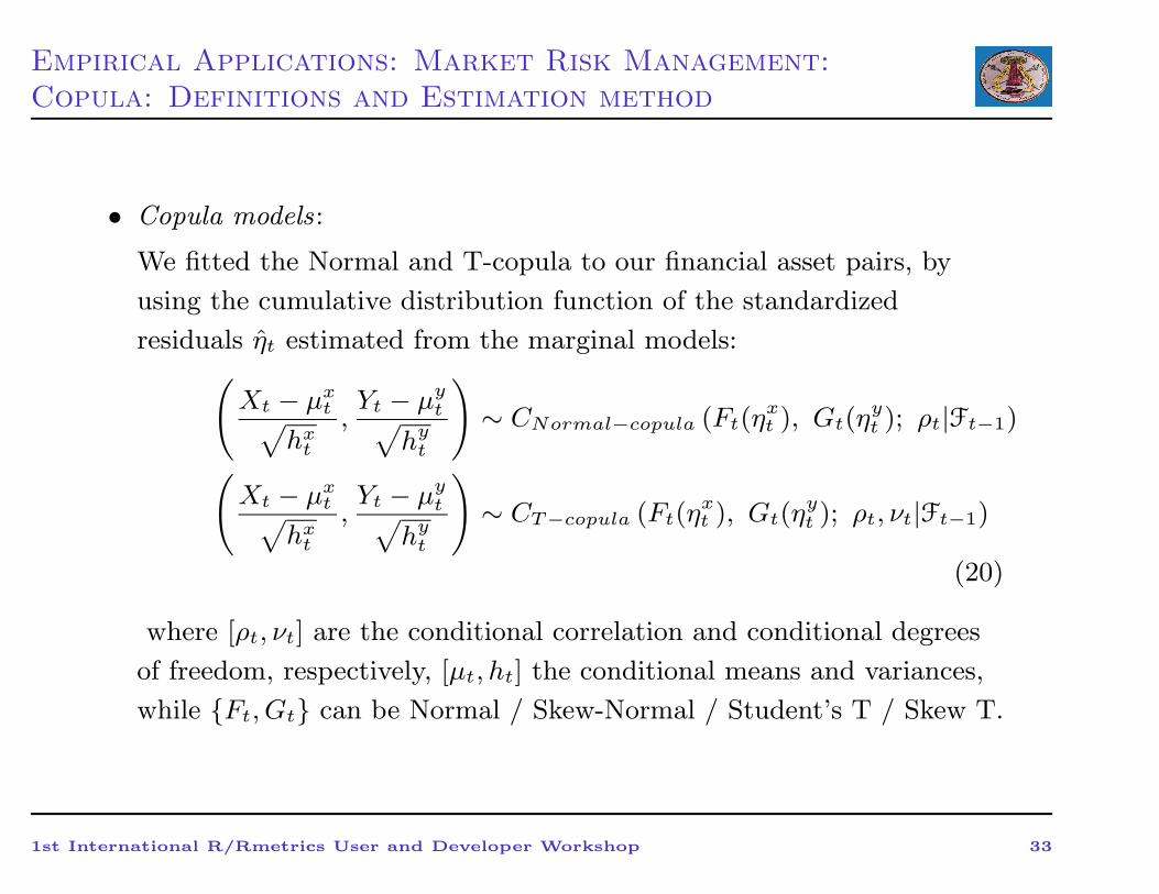
• Copula models:
We fitted the Normal and T-copula to our financial asset pairs, by
using the cumulative distribution function of the standardized
residuals ηt estimated from the marginal models:(
Xt − µxt
√
hxt
,Yt − µy
t√
hyt
)
∼ CNormal−copula (Ft(ηxt ), Gt(η
yt ); ρt|Ft−1)
(
Xt − µxt
√
hxt
,Yt − µy
t√
hyt
)
∼ CT−copula (Ft(ηxt ), Gt(η
yt ); ρt, νt|Ft−1)
(20)
where [ρt, νt] are the conditional correlation and conditional degrees
of freedom, respectively, [µt, ht] the conditional means and variances,
while {Ft, Gt} can be Normal / Skew-Normal / Student’s T / Skew T.
1st International R/Rmetrics User and Developer Workshop 33
Empirical Applications: Market Risk Management:
Value at Risk Applications
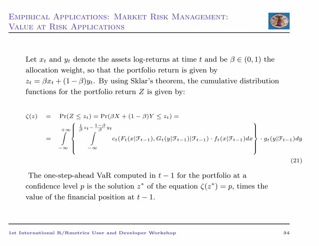
Let xt and yt denote the assets log-returns at time t and be β ∈ (0, 1) the
allocation weight, so that the portfolio return is given by
zt = βxt + (1− β)yt. By using Sklar’s theorem, the cumulative distribution
functions for the portfolio return Z is given by:
ζ(z) = Pr(Z ≤ zt) = Pr(βX + (1 − β)Y ≤ zt) =
=
+∞∫
−∞
1β
zt−1−β
βyt
∫
−∞
ct(Ft(x|Ft−1), Gt(y|Ft−1)|Ft−1) · ft(x|Ft−1)dx
· gt(y|Ft−1)dy
(21)
The one-step-ahead VaR computed in t− 1 for the portfolio at a
confidence level p is the solution z∗ of the equation ζ(z∗) = p, times the
value of the financial position at t− 1.
1st International R/Rmetrics User and Developer Workshop 34
Empirical Applications: Market Risk Management:
Value at Risk Applications
⇒ The computation of the one-step-ahead VaR requires the solution of the
previous double integral: However, while this solution is feasible in the
bivariate case, it becomes computationally problematic when the number
of assets is much higher than two.
⇒ This is why we prefer to compute the VaR using a simple Monte Carlo
simulation as widely used in quantitative finance and option pricing. See
Jorion (2000) for a discussion of Monte Carlo techniques in VaR
applications.
⇒ Following this solution, we generate a large number of one-day-ahead
returns {xt, yt} for the two assets, by simulating 100,000 random returns
with the conditional distribution function (21) and we revaluate the
portfolio at time t. We then determine the Value at Risk at a given
confidence level p, by simply taking the empirical quantile at p of the
simulated portfolio profit and loss distribution.
1st International R/Rmetrics User and Developer Workshop 35
Empirical Applications: Market Risk Management:
Value at Risk Applications
The detailed steps of the procedure for estimating the 95%, 99% VaR over
a one-day holding period are the following:
1. Let consider the portfolio z which contains one position for each of the
2 risk factors (or assets), whose value at time t− 1 is:
Pz,t−1 = Px,t−1 + Py,t−1
where Px,t−1, Py,t−1 are the market prices of the two assets at time
t− 1.
2. We simulate j = 100,000 MC scenarios for each asset log-returns,
{xj,t , yj,t}, over the time horizon [t− 1, t], using the conditional joint
distributional function (3.1).
(a) First, we have to simulate a j random variate (uj,x, uj,y)′ from the
copula Ct(·). See Cherubini et al. (2004), for a discussion about
copula simulation.
1st International R/Rmetrics User and Developer Workshop 36
Empirical Applications: Market Risk Management:
Value at Risk Applications
(b) Second, we get the standardized asset log-returns by using the
inverse functions of the estimated marginals, which can be Normal
/ Skew-Normal / T-Student / Skew-T, as described in section 2.2
and Appendix A:
Qj = (qj,x, qj,y)′ = (Ft−1
(uj,x); Gt−1
(uj,y))
(c) Third, we rescale the standardized assets log-returns by using the
forecasted means and variances, estimated with AR-GARCH
models as described in section 2.3.2:
{xj,t, yj,t} =
(
µx,t + qj,x ·√
hx,t, µy,t + qj,y ·√
hy,t
)
(d) Finally, we repeat this procedure for j = 100, 000 times.
3. By using these 100,000 scenarios, the portfolio is being revaluated at
time t, that is:
P jz,t = Px,t−1 · exp(xj,t) + Py,t−1 · exp(yj,t), j = 1...100, 000
1st International R/Rmetrics User and Developer Workshop 37
Empirical Applications: Market Risk Management:
Value at Risk Applications
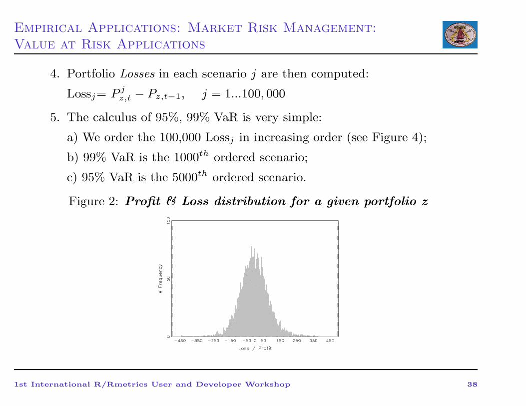
4. Portfolio Losses in each scenario j are then computed:
Lossj= P jz,t − Pz,t−1, j = 1...100, 000
5. The calculus of 95%, 99% VaR is very simple:
a) We order the 100,000 Lossj in increasing order (see Figure 4);
b) 99% VaR is the 1000th ordered scenario;
c) 95% VaR is the 5000th ordered scenario.
Figure 2: Profit & Loss distribution for a given portfolio z
1st International R/Rmetrics User and Developer Workshop 38
Empirical Applications: Market Risk Management:
Value at Risk Applications
Traditional risk measurement models assume that the risk factors are
multivariate normal: empirical evidence shows the importance of skewness,
kurtosis, dynamic dependence (Tsay, 2002).
→ Starting from these stylized facts and theoretical background, I
introduced a model to generate scenarios for portfolio risk factors from
different conditional multivariate distributions.
Four elements were considered:
1. The choice of the marginals distribution;
2. The specification of the conditional moments of the marginals;
3. The choice of the copula to link the marginals into a proper
multivariate distribution;
4. The specification of the conditional copula parameters
1st International R/Rmetrics User and Developer Workshop 39
Empirical Applications: Market Risk Management:
Value at Risk Applications
To evaluate how important these four elements are, I generate out-of-
sample VaR forecasts for three portfolios (SP500-DAX, SP500-NIKKEI225,
NIKKEI225-DAX), by simulating 100.000 MC scenarios out of the
conditional joint density (11) with these different possible choices:
1. marginals distribution: Normal, Skew-Normal, Student´s T, Skew-T;
2. conditional moments Specification:
• Constant Mean / AR(1) process;
• Constant Variance / GARCH(1,1) process / T-GARCH(1,1)
• Constant / Dynamic Degrees of Freedom;
• Constant / Dynamic Skewness parameters;
3. Normal copula / T - copula;
4. Constant / Dynamic copula parameters
1st International R/Rmetrics User and Developer Workshop 40
Empirical Applications: Market Risk Management:
Empirical analysis
→ I generate portfolio Value at Risk forecasts at the 95 % - 99 %
confidence levels. The predicted one-step-ahead VaR forecasts are then
compared with the observed portfolio losses.
→ The initialization sample is given by the first 700 observations.
→ Recursive estimation from the 700th to the 1699th observation (for a
total of 1000 observations).
→ The performance of the competing models over these 1000 observations
is assessed using the following back-testing techniques:
• Kupiec’s unconditional coverage test;
• Christoffersen’s conditional coverage test;
• Loss functions to evaluate VaR forecasts accuracy.
1st International R/Rmetrics User and Developer Workshop 41
Empirical Applications: Market Risk Management:
Empirical analysis
• Diagnostics for real VaR exceedances
1. Kupiec’s test: Following binomial theory, the probability of
observing N failures out of T observations is (1-p)T−NpN , so that the
test of the null hypothesis H0: p = p∗ is given by a LR test statistic:
LR = 2 · ln[(1 − p∗)T−Np∗N
] + 2 · ln[(1 −N/T )T−N (N/T )N ]
2. Christoffersen’s test: . Its main advantage over the previous
statistic is that it takes account of any conditionality in our forecast:
for example, if volatilities are low in some period and high in others,
the VaR forecast should respond to this clustering event.
LRCC = −2 ln[(1−p)T−NpN ]+2 ln[(1−π01)n00πn01
01 (1−π11)n10πn11
11 ]
where nij is the number of observations with value i followed by j for
i, j = 0, 1 and
πij =nij
∑
j nij
1st International R/Rmetrics User and Developer Workshop 42
Empirical Applications: Market Risk Management:
Empirical analysis
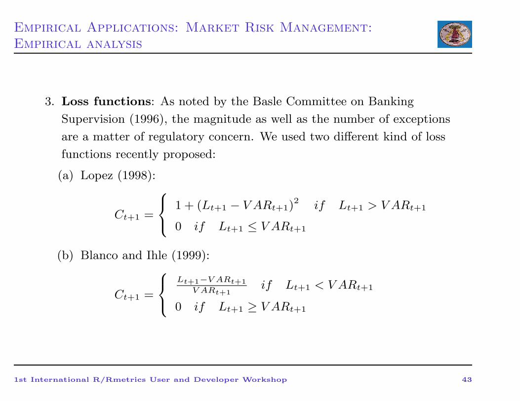
3. Loss functions: As noted by the Basle Committee on Banking
Supervision (1996), the magnitude as well as the number of exceptions
are a matter of regulatory concern. We used two different kind of loss
functions recently proposed:
(a) Lopez (1998):
Ct+1 =
1 + (Lt+1 − V ARt+1)2 if Lt+1 > V ARt+1
0 if Lt+1 ≤ V ARt+1
(b) Blanco and Ihle (1999):
Ct+1 =
Lt+1−V ARt+1
V ARt+1if Lt+1 < V ARt+1
0 if Lt+1 ≥ V ARt+1
1st International R/Rmetrics User and Developer Workshop 43

Empirical Applications: Market Risk Management:
Empirical analysis
Table 1 DYNAMIC NORMAL COPULASP500 - DAX
95% 99%
Marg.
Distr.
Moment specification N/T pUC pCC N/T pUC pCC
NORMAL Constant: Mean, Variance 11,59% 0,000 0,000 5,39% 0,000 0,000
AR(1) Constant, Variance 11,49% 0,000 0,000 5,19% 0,000 0,000
AR(1) GARCH(1,1) 6,69% 0,019 0,058 1,40% 0,232 0,396
AR(1) T-GARCH(1,1) 5,89% 0,206 0,303 0,70% 0,312 0,567
SKEW- Constant: Mean, Variance, Skewness 10,49% 0,000 0,000 4,60% 0,000 0,000
NORMAL AR(1) Constant: Variance, Skewness 10,99% 0,000 0,000 4,70% 0,000 0,000
AR(1) GARCH(1,1) Const. Skew. 5,79% 0,260 0,469 1,10% 0,757 0,834
AR(1) T-GARCH(1,1) Const. Skew. 5,09% 0,891 0,910 0,60% 0,169 0,372
AR(1) T-GARCH(1,1) Dyn. Skewness 4,30% 0,295 0,550 0,20% 0,002 0,008
STUD.’s Constant: Mean, Variance, D.o.F. 12,59% 0,000 0,000 4,10% 0,000 0,000
T AR(1) Constant: Variance, D.o.F. 13,89% 0,000 0,000 4,30% 0,000 0,000
AR(1) GARCH(1,1) Constant D.o.F. 8,19% 0,000 0,000 1,10% 0,757 0,834
AR(1) T-GARCH(1,1) Const. D.o.F. 7,69% 0,000 0,001 0,70% 0,312 0,567
AR(1) T-GARCH(1,1) Dynamic D.o.F. 6,99% 0,006 0,019 1,00% 0,997 0,895
SKEW Const: Mean, Variance, Skew., D.o.F. 11,99% 0,000 0,000 3,50% 0,000 0,000
T AR(1) Const: Variance, Skew, D.o.F. 12,89% 0,000 0,000 4,10% 0,000 0,000
AR(1) GARCH(1,1) C. Skew, D.o.F. 6,89% 0,009 0,026 0,80% 0,508 0,747
AR(1) T-GARCH(1,1) C. Skew, D.o.F. 6,19% 0,094 0,193 0,50% 0,078 0,206
AR(1)T-GARCH(1,1)D. Skew, C. D.o.F. 5,09% 0,891 0,653 0,40% 0,030 0,093
AR(1)T-GARCH(1,1)D. Skew, D. D.o.F. 4,50% 0,457 0,312 0,30% 0,009 0,032
1st International R/Rmetrics User and Developer Workshop 44
Empirical Applications: Market Risk Management:
Empirical analysis
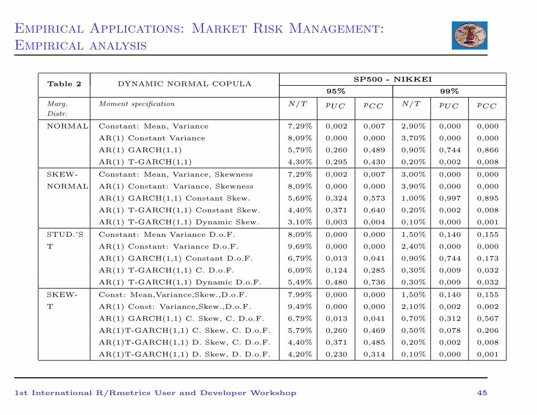
Table 2 DYNAMIC NORMAL COPULASP500 - NIKKEI
95% 99%
Marg.
Distr.
Moment specification N/T pUC pCC N/T pUC pCC
NORMAL Constant: Mean, Variance 7,29% 0,002 0,007 2,90% 0,000 0,000
AR(1) Constant Variance 8,09% 0,000 0,000 3,70% 0,000 0,000
AR(1) GARCH(1,1) 5,79% 0,260 0,489 0,90% 0,744 0,866
AR(1) T-GARCH(1,1) 4,30% 0,295 0,430 0,20% 0,002 0,008
SKEW- Constant: Mean, Variance, Skewness 7,29% 0,002 0,007 3,00% 0,000 0,000
NORMAL AR(1) Constant: Variance, Skewness 8,09% 0,000 0,000 3,90% 0,000 0,000
AR(1) GARCH(1,1) Constant Skew. 5,69% 0,324 0,573 1,00% 0,997 0,895
AR(1) T-GARCH(1,1) Constant Skew. 4,40% 0,371 0,640 0,20% 0,002 0,008
AR(1) T-GARCH(1,1) Dynamic Skew. 3,10% 0,003 0,004 0,10% 0,000 0,001
STUD.’S Constant: Mean Variance D.o.F. 8,09% 0,000 0,000 1,50% 0,140 0,155
T AR(1) Constant: Variance D.o.F. 9,69% 0,000 0,000 2,40% 0,000 0,000
AR(1) GARCH(1,1) Constant D.o.F. 6,79% 0,013 0,041 0,90% 0,744 0,173
AR(1) T-GARCH(1,1) C. D.o.F. 6,09% 0,124 0,285 0,30% 0,009 0,032
AR(1) T-GARCH(1,1) Dynamic D.o.F. 5,49% 0,480 0,736 0,30% 0,009 0,032
SKEW- Const: Mean,Variance,Skew.,D.o.F. 7,99% 0,000 0,000 1,50% 0,140 0,155
T AR(1) Const: Variance,Skew.,D.o.F. 9,49% 0,000 0,000 2,10% 0,002 0,002
AR(1) GARCH(1,1) C. Skew, C. D.o.F. 6,79% 0,013 0,041 0,70% 0,312 0,567
AR(1)T-GARCH(1,1) C. Skew, C. D.o.F. 5,79% 0,260 0,469 0,50% 0,078 0,206
AR(1)T-GARCH(1,1) D. Skew, C. D.o.F. 4,40% 0,371 0,485 0,20% 0,002 0,008
AR(1)T-GARCH(1,1) D. Skew, D. D.o.F. 4,20% 0,230 0,314 0,10% 0,000 0,001
1st International R/Rmetrics User and Developer Workshop 45
Empirical Applications: Market Risk Management:
Empirical analysis
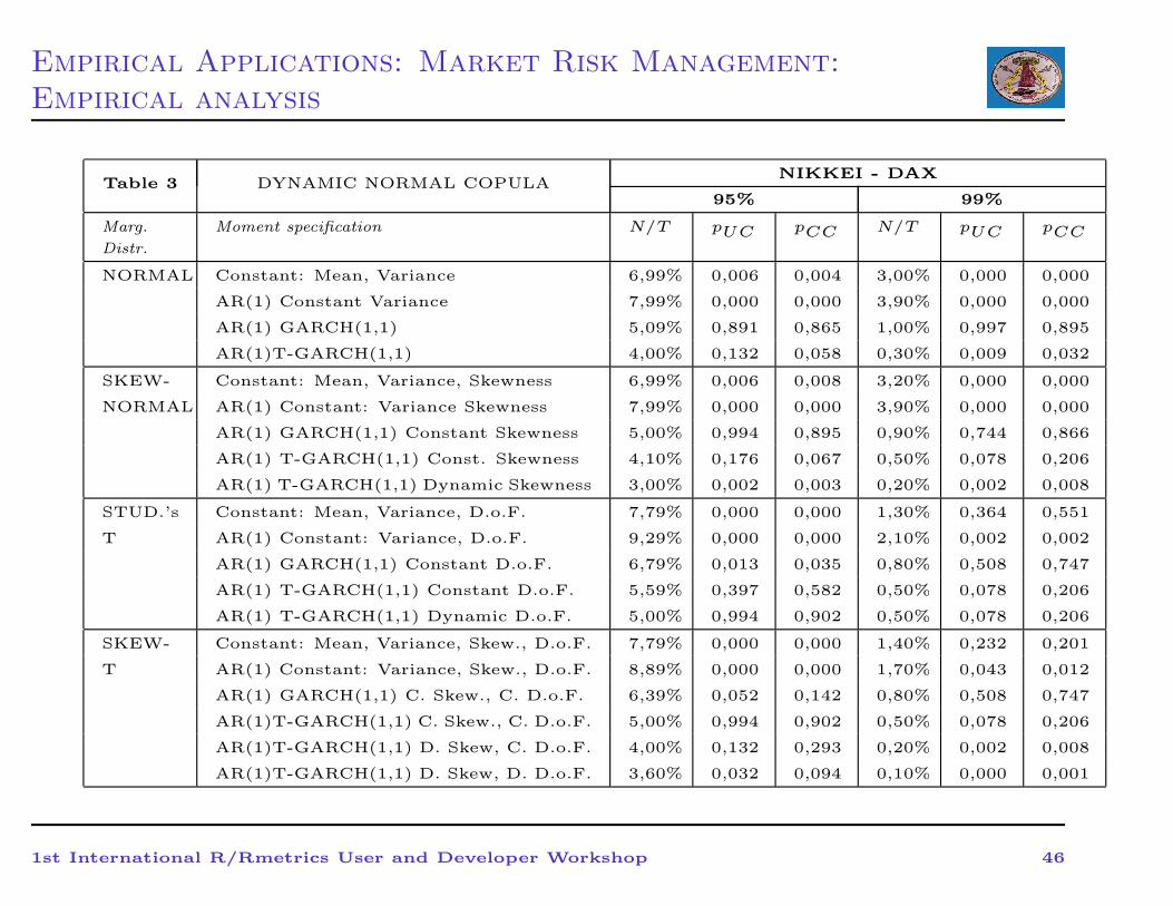
Table 3 DYNAMIC NORMAL COPULANIKKEI - DAX
95% 99%
Marg.
Distr.
Moment specification N/T pUC pCC N/T pUC pCC
NORMAL Constant: Mean, Variance 6,99% 0,006 0,004 3,00% 0,000 0,000
AR(1) Constant Variance 7,99% 0,000 0,000 3,90% 0,000 0,000
AR(1) GARCH(1,1) 5,09% 0,891 0,865 1,00% 0,997 0,895
AR(1)T-GARCH(1,1) 4,00% 0,132 0,058 0,30% 0,009 0,032
SKEW- Constant: Mean, Variance, Skewness 6,99% 0,006 0,008 3,20% 0,000 0,000
NORMAL AR(1) Constant: Variance Skewness 7,99% 0,000 0,000 3,90% 0,000 0,000
AR(1) GARCH(1,1) Constant Skewness 5,00% 0,994 0,895 0,90% 0,744 0,866
AR(1) T-GARCH(1,1) Const. Skewness 4,10% 0,176 0,067 0,50% 0,078 0,206
AR(1) T-GARCH(1,1) Dynamic Skewness 3,00% 0,002 0,003 0,20% 0,002 0,008
STUD.’s Constant: Mean, Variance, D.o.F. 7,79% 0,000 0,000 1,30% 0,364 0,551
T AR(1) Constant: Variance, D.o.F. 9,29% 0,000 0,000 2,10% 0,002 0,002
AR(1) GARCH(1,1) Constant D.o.F. 6,79% 0,013 0,035 0,80% 0,508 0,747
AR(1) T-GARCH(1,1) Constant D.o.F. 5,59% 0,397 0,582 0,50% 0,078 0,206
AR(1) T-GARCH(1,1) Dynamic D.o.F. 5,00% 0,994 0,902 0,50% 0,078 0,206
SKEW- Constant: Mean, Variance, Skew., D.o.F. 7,79% 0,000 0,000 1,40% 0,232 0,201
T AR(1) Constant: Variance, Skew., D.o.F. 8,89% 0,000 0,000 1,70% 0,043 0,012
AR(1) GARCH(1,1) C. Skew., C. D.o.F. 6,39% 0,052 0,142 0,80% 0,508 0,747
AR(1)T-GARCH(1,1) C. Skew., C. D.o.F. 5,00% 0,994 0,902 0,50% 0,078 0,206
AR(1)T-GARCH(1,1) D. Skew, C. D.o.F. 4,00% 0,132 0,293 0,20% 0,002 0,008
AR(1)T-GARCH(1,1) D. Skew, D. D.o.F. 3,60% 0,032 0,094 0,10% 0,000 0,001
1st International R/Rmetrics User and Developer Workshop 46
Empirical Applications: Market Risk Management:
Empirical analysis
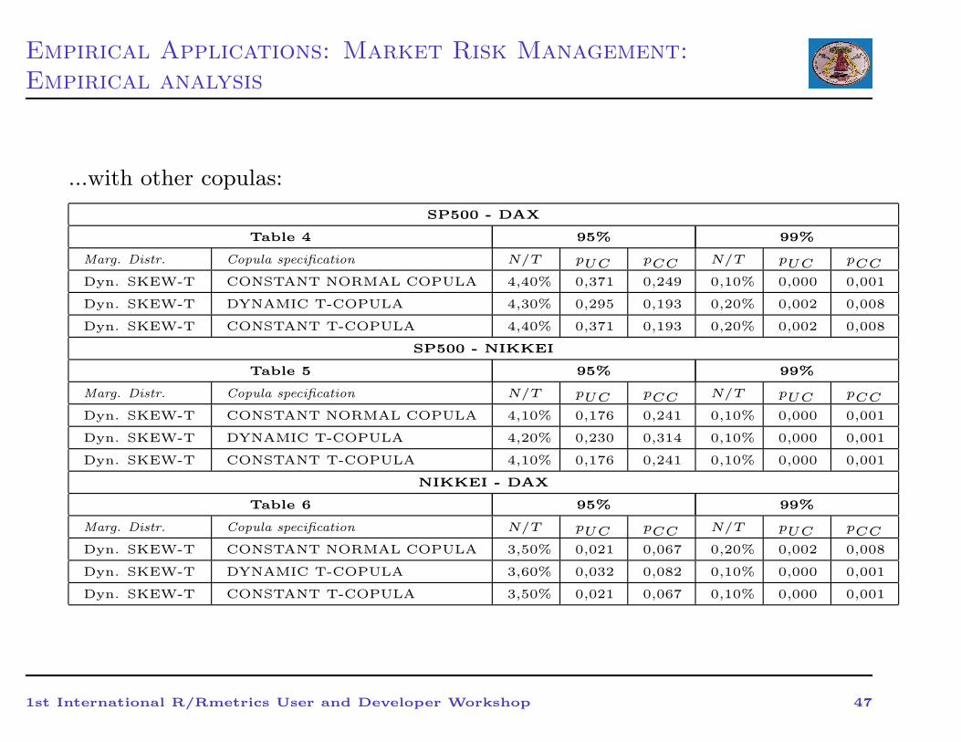
...with other copulas:
SP500 - DAX
Table 4 95% 99%
Marg. Distr. Copula specification N/T pUC pCC N/T pUC pCC
Dyn. SKEW-T CONSTANT NORMAL COPULA 4,40% 0,371 0,249 0,10% 0,000 0,001
Dyn. SKEW-T DYNAMIC T-COPULA 4,30% 0,295 0,193 0,20% 0,002 0,008
Dyn. SKEW-T CONSTANT T-COPULA 4,40% 0,371 0,193 0,20% 0,002 0,008
SP500 - NIKKEI
Table 5 95% 99%
Marg. Distr. Copula specification N/T pUC pCC N/T pUC pCC
Dyn. SKEW-T CONSTANT NORMAL COPULA 4,10% 0,176 0,241 0,10% 0,000 0,001
Dyn. SKEW-T DYNAMIC T-COPULA 4,20% 0,230 0,314 0,10% 0,000 0,001
Dyn. SKEW-T CONSTANT T-COPULA 4,10% 0,176 0,241 0,10% 0,000 0,001
NIKKEI - DAX
Table 6 95% 99%
Marg. Distr. Copula specification N/T pUC pCC N/T pUC pCC
Dyn. SKEW-T CONSTANT NORMAL COPULA 3,50% 0,021 0,067 0,20% 0,002 0,008
Dyn. SKEW-T DYNAMIC T-COPULA 3,60% 0,032 0,082 0,10% 0,000 0,001
Dyn. SKEW-T CONSTANT T-COPULA 3,50% 0,021 0,067 0,10% 0,000 0,001
1st International R/Rmetrics User and Developer Workshop 47
Empirical Applications: Market Risk Management:
Empirical analysis
• Empirical Results
1. The GARCH specification for the variance is absolutely fundamental
to have good VaR forecasts, whatever the marginal distribution is;
2. The asymmetric GARCH specification is important to get precise VaR
estimates at the 95% confidence level. However, it can produce
conservative estimates at the 99% level when dealing with strongly
leptokurtic assets and the normal (or skew-normal) distribution is
used;
3. The AR specification of the mean is not relevant in all cases;
4. The GARCH specification seems to model most of the leptokurtosis
present in the data. However, when the assets are strongly leptokurtic,
a Skew-T distribution is the best choice (similarly to point 2.);
1st International R/Rmetrics User and Developer Workshop 48
Empirical Applications: Market Risk Management:
Empirical analysis
5. Using a Student’s T distribution with strongly skewed assets can
produce very aggressive VaR forecasts at the 95% level;
6. The Skew-T and Skew-Normal distributions present the most precise
VaR forecasts, according to the tests and Loss functions used;
7. Allowing for dynamics in the skewness and degrees of freedom
parameters produces more conservative VaR forecasts in almost all
cases;
8. The type of copula as well as the dynamics in its parameters are not
relevant : a simple normal copula with constant correlation resulted to
be sufficient in all cases.
1st International R/Rmetrics User and Developer Workshop 49
Empirical Applications: Market Risk Management:
Empirical analysis
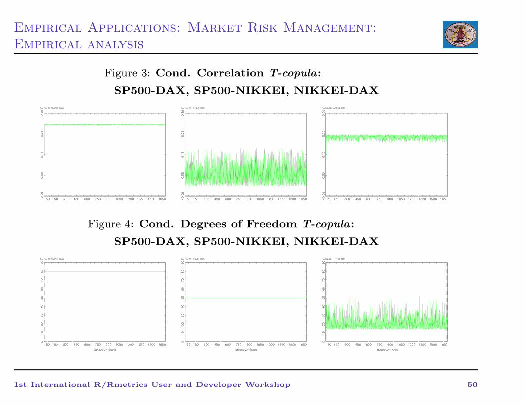
Figure 3: Cond. Correlation T-copula:
SP500-DAX, SP500-NIKKEI, NIKKEI-DAX
Figure 4: Cond. Degrees of Freedom T-copula:
SP500-DAX, SP500-NIKKEI, NIKKEI-DAX
1st International R/Rmetrics User and Developer Workshop 50
Empirical Applications: Market Risk Management:
Conclusions and extensions
• Joint conditional normal distribution can give poor VaR
forecasts.
• Copulae proved to be a good solution for modeling dependence .
• ...but the choice of marginals is still the most important decision!
→ Skew - Normal or Skew - T
• Extend this framework to the Multivariate case, where copula’s
conditional correlation matrix is modelled with a DCC model
(Patton et al, 2004), or by using decomposition models like
Rydberg and Shephard (2003)
1st International R/Rmetrics User and Developer Workshop 51
Empirical Applications - Market Risk Management for
Multivariate Portfolios: Introduction
Daul, Giorgi, Lindskog, and McNeil (2003), Demarta and McNeil (2005)
and Mc-Neil, Frey, and Embrechts (2005) underlined the ability of the
grouped t-copula to model the dependence present in a large set of
financial assets into account.
We extend their methodology by allowing the copula dependence structure
to be time-varying and we show how to estimate its parameters.
Furthermore, we prove the consistency and asymptotic normality of this
estimator under some special cases and we examine its finite samples
properties via simulations.
Finally, we apply this methodology for the estimation of the VaR of a
portfolio composed of thirty assets.
1st International R/Rmetrics User and Developer Workshop 52
Market Risk Management for Multivariate Portfolios: Dynamic
Grouped-T Copula Modelling: Definition and Estimation
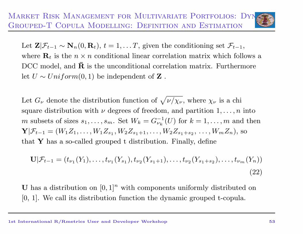
Let Z|Ft−1 ∼ Nn(0,Rt), t = 1, . . . T , given the conditioning set Ft−1,
where Rt is the n× n conditional linear correlation matrix which follows a
DCC model, and R is the unconditional correlation matrix. Furthermore
let U ∼ Uniform(0, 1) be independent of Z .
Let Gν denote the distribution function of√
ν/χν , where χν is a chi
square distribution with ν degrees of freedom, and partition 1, . . . , n into
m subsets of sizes s1, . . . , sm. Set Wk = G−1νk
(U) for k = 1, . . . ,m and then
Y|Ft−1 = (W1Z1, . . . ,W1Zs1 ,W2Zs1+1, . . . ,W2Zs1+s2 , . . . ,WmZn), so
that Y has a so-called grouped t distribution. Finally, define
U|Ft−1 = (tν1(Y1), . . . , tν1(Ys1), tν2(Ys1+1), . . . , tν2(Ys1+s2), . . . , tνm(Yn))
(22)
U has a distribution on [0, 1]n with components uniformly distributed on
[0, 1]. We call its distribution function the dynamic grouped t-copula.
1st International R/Rmetrics User and Developer Workshop 53
Market Risk Management for Multivariate Portfolios: Dynamic
Grouped-T Copula Modelling: Definition and Estimation
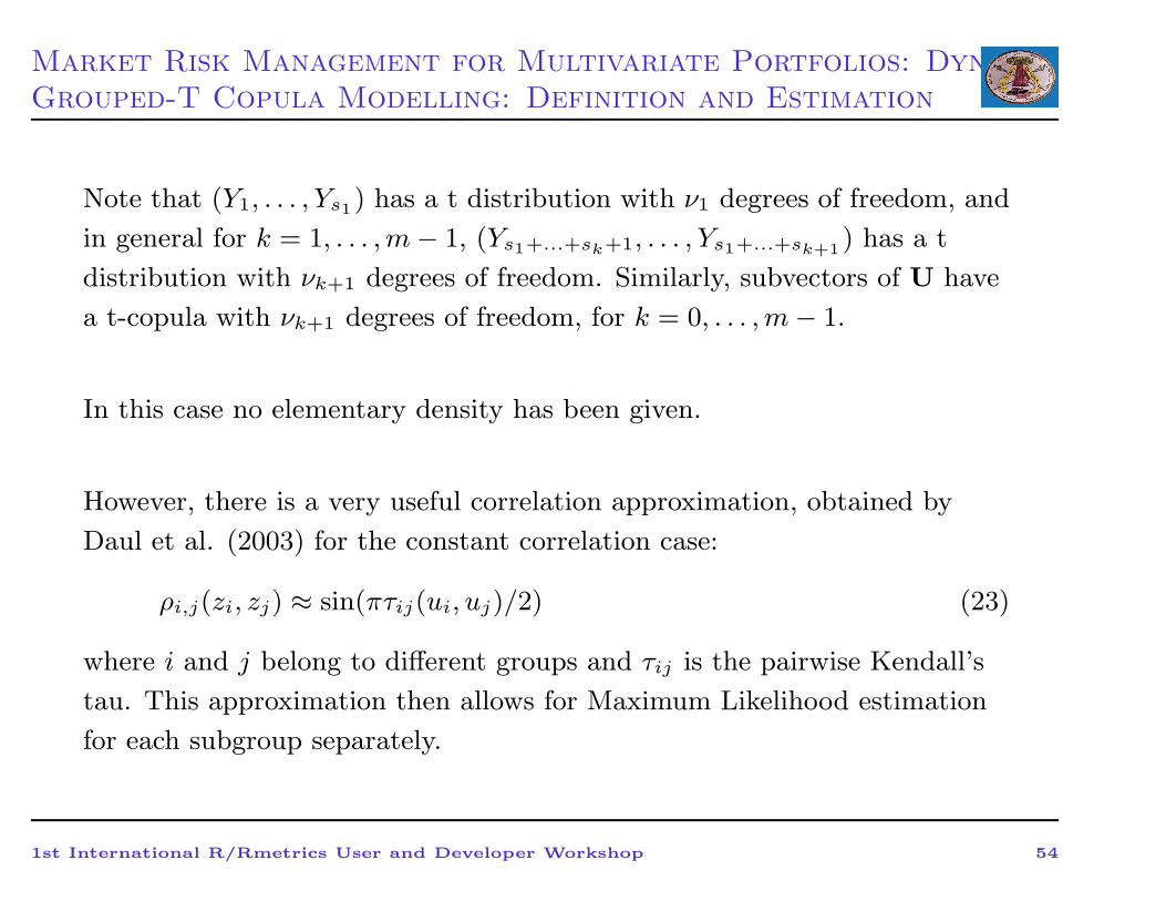
Note that (Y1, . . . , Ys1) has a t distribution with ν1 degrees of freedom, and
in general for k = 1, . . . ,m− 1, (Ys1+...+sk+1, . . . , Ys1+...+sk+1) has a t
distribution with νk+1 degrees of freedom. Similarly, subvectors of U have
a t-copula with νk+1 degrees of freedom, for k = 0, . . . ,m− 1.
In this case no elementary density has been given.
However, there is a very useful correlation approximation, obtained by
Daul et al. (2003) for the constant correlation case:
ρi,j(zi, zj) ≈ sin(πτij(ui, uj)/2) (23)
where i and j belong to different groups and τij is the pairwise Kendall’s
tau. This approximation then allows for Maximum Likelihood estimation
for each subgroup separately.
1st International R/Rmetrics User and Developer Workshop 54
Market Risk Management for Multivariate Portfolios: Dynamic
Grouped-T Copula Modelling: Definition and Estimation
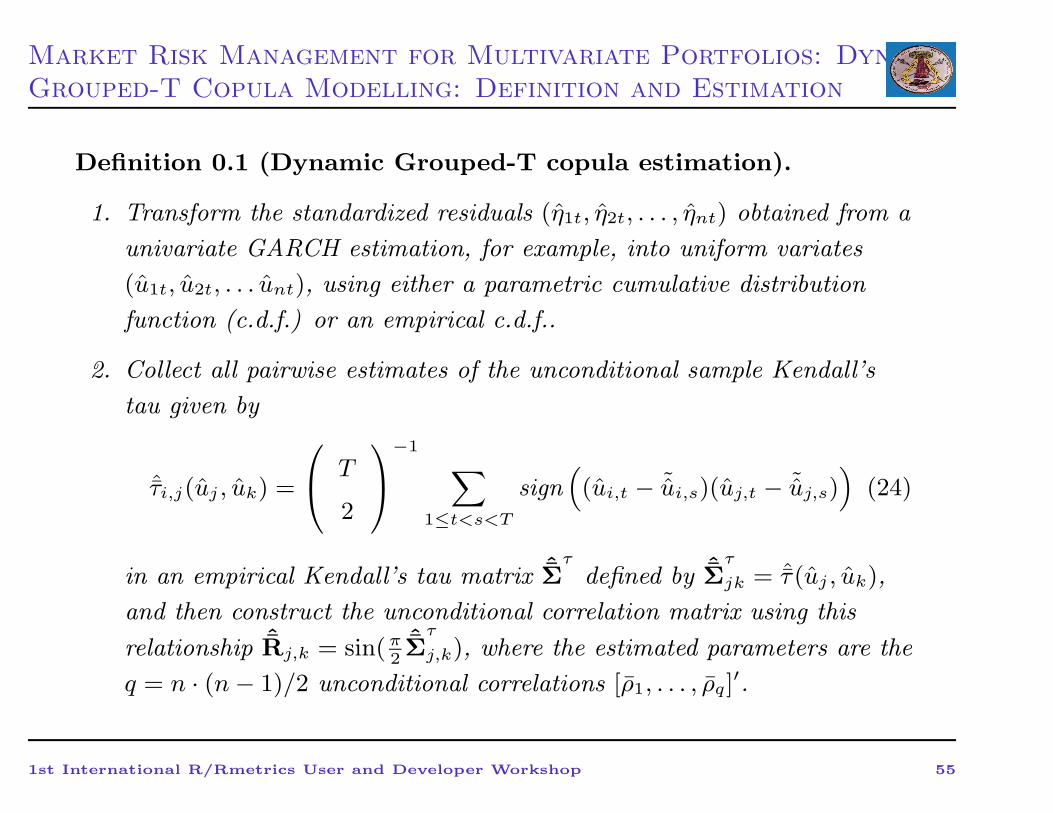
Definition 0.1 (Dynamic Grouped-T copula estimation).
1. Transform the standardized residuals (η1t, η2t, . . . , ηnt) obtained from a
univariate GARCH estimation, for example, into uniform variates
(u1t, u2t, . . . unt), using either a parametric cumulative distribution
function (c.d.f.) or an empirical c.d.f..
2. Collect all pairwise estimates of the unconditional sample Kendall’s
tau given by
ˆτi,j(uj , uk) =
T
2
−1∑
1≤t<s<T
sign(
(ui,t − ˜ui,s)(uj,t − ˜uj,s))
(24)
in an empirical Kendall’s tau matrix ˆΣτ
defined by ˆΣτ
jk = ˆτ(uj , uk),
and then construct the unconditional correlation matrix using this
relationship ˆRj,k = sin(π2ˆΣ
τ
j,k), where the estimated parameters are the
q = n · (n− 1)/2 unconditional correlations [ρ1, . . . , ρq]′.
1st International R/Rmetrics User and Developer Workshop 55
Market Risk Management for Multivariate Portfolios: Dynamic
Grouped-T Copula Modelling: Definition and Estimation
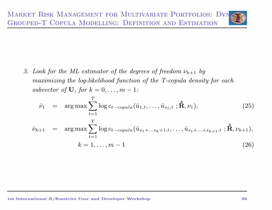
3. Look for the ML estimator of the degrees of freedom νk+1 by
maximizing the log-likelihood function of the T-copula density for each
subvector of U, for k = 0, . . . ,m− 1:
ν1 = arg max
T∑
t=1
log ct−copula(u1,t, . . . , us1,t ; ˆR, ν1), (25)
νk+1 = arg max
T∑
t=1
log ct−copula(us1+...sk+1,t, . . . , us1+...+sk+1,t ; ˆR, νk+1),
k = 1, . . . ,m− 1 (26)
1st International R/Rmetrics User and Developer Workshop 56
Market Risk Management for Multivariate Portfolios: Dynamic
Grouped-T Copula Modelling: Definition and Estimation
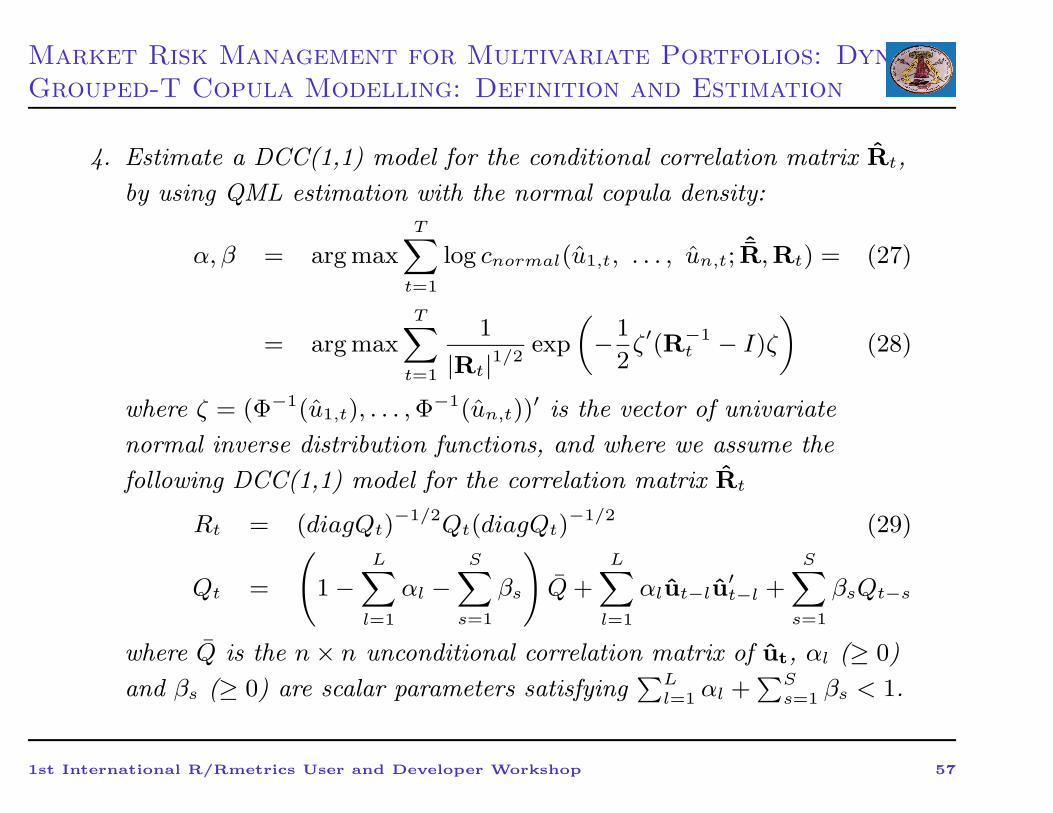
4. Estimate a DCC(1,1) model for the conditional correlation matrix Rt,
by using QML estimation with the normal copula density:
α, β = arg max
T∑
t=1
log cnormal(u1,t, . . . , un,t;ˆR,Rt) = (27)
= arg max
T∑
t=1
1
|Rt|1/2exp
(
−1
2ζ′(R−1
t − I)ζ
)
(28)
where ζ = (Φ−1(u1,t), . . . ,Φ−1(un,t))
′ is the vector of univariate
normal inverse distribution functions, and where we assume the
following DCC(1,1) model for the correlation matrix Rt
Rt = (diagQt)−1/2Qt(diagQt)
−1/2 (29)
Qt =
(
1 −L∑
l=1
αl −S∑
s=1
βs
)
Q+
L∑
l=1
αlut−lu′t−l +
S∑
s=1
βsQt−s
where Q is the n× n unconditional correlation matrix of ut, αl (≥ 0)
and βs (≥ 0) are scalar parameters satisfying∑L
l=1 αl +∑S
s=1 βs < 1.
1st International R/Rmetrics User and Developer Workshop 57
Empirical Applications - Market Risk Management for
Multivariate Portfolios: Asymptotic Properties
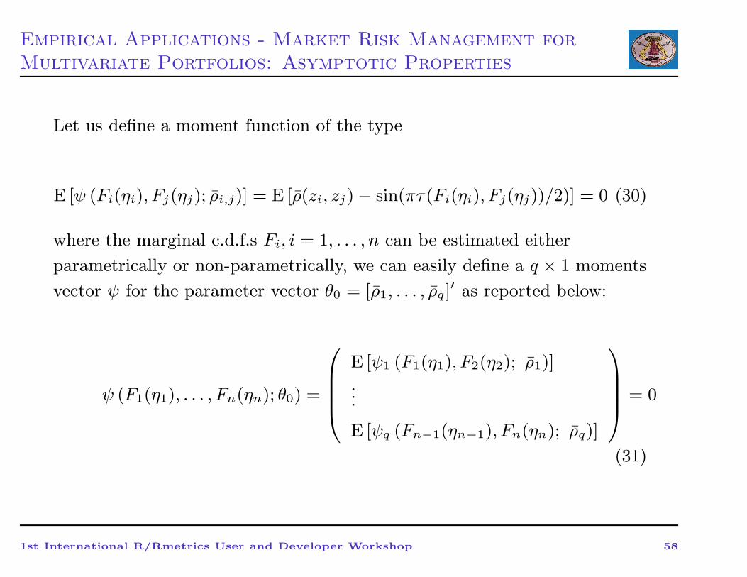
Let us define a moment function of the type
E [ψ (Fi(ηi), Fj(ηj); ρi,j)] = E [ρ(zi, zj) − sin(πτ(Fi(ηi), Fj(ηj))/2)] = 0 (30)
where the marginal c.d.f.s Fi, i = 1, . . . , n can be estimated either
parametrically or non-parametrically, we can easily define a q × 1 moments
vector ψ for the parameter vector θ0 = [ρ1, . . . , ρq]′ as reported below:
ψ (F1(η1), . . . , Fn(ηn); θ0) =
E [ψ1 (F1(η1), F2(η2); ρ1)]
...
E [ψq (Fn−1(ηn−1), Fn(ηn); ρq)]
= 0
(31)
1st International R/Rmetrics User and Developer Workshop 58
Empirical Applications - Market Risk Management for
Multivariate Portfolios: Asymptotic Properties
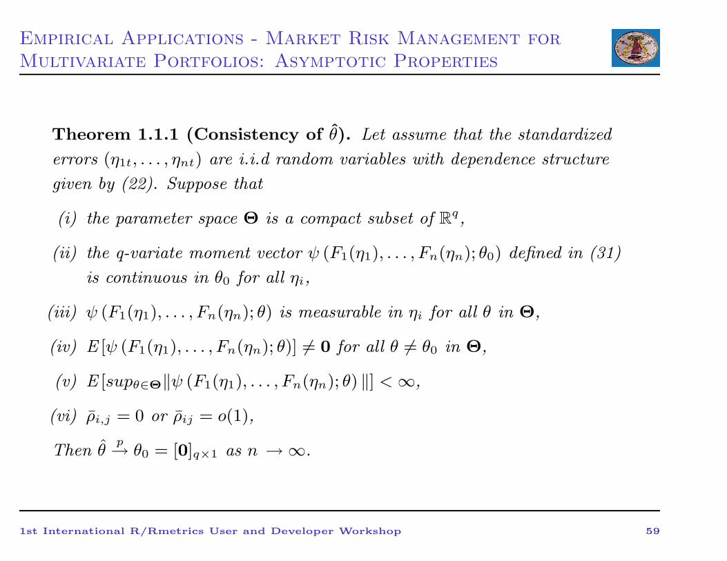
Theorem 1.1.1 (Consistency of θ). Let assume that the standardized
errors (η1t, . . . , ηnt) are i.i.d random variables with dependence structure
given by (22). Suppose that
(i) the parameter space Θ is a compact subset of Rq,
(ii) the q-variate moment vector ψ (F1(η1), . . . , Fn(ηn); θ0) defined in (31)
is continuous in θ0 for all ηi,
(iii) ψ (F1(η1), . . . , Fn(ηn); θ) is measurable in ηi for all θ in Θ,
(iv) E [ψ (F1(η1), . . . , Fn(ηn); θ)] 6= 0 for all θ 6= θ0 in Θ,
(v) E [supθ∈Θ‖ψ (F1(η1), . . . , Fn(ηn); θ) ‖] <∞,
(vi) ρi,j = 0 or ρij = o(1),
Then θp→ θ0 = [0]q×1 as n → ∞.
1st International R/Rmetrics User and Developer Workshop 59
Empirical Applications - Market Risk Management for
Multivariate Portfolios: Asymptotic Properties
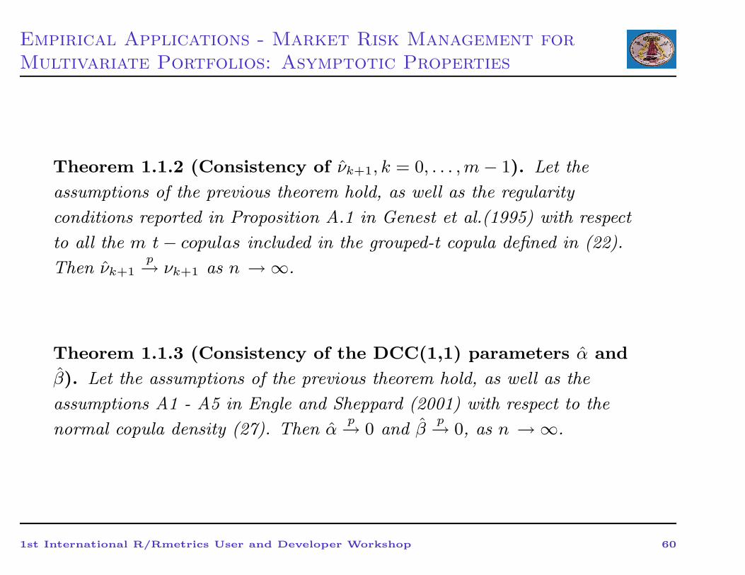
Theorem 1.1.2 (Consistency of νk+1, k = 0, . . . ,m− 1). Let the
assumptions of the previous theorem hold, as well as the regularity
conditions reported in Proposition A.1 in Genest et al.(1995) with respect
to all the m t− copulas included in the grouped-t copula defined in (22).
Then νk+1p→ νk+1 as n → ∞.
Theorem 1.1.3 (Consistency of the DCC(1,1) parameters α and
β). Let the assumptions of the previous theorem hold, as well as the
assumptions A1 - A5 in Engle and Sheppard (2001) with respect to the
normal copula density (27). Then αp→ 0 and β
p→ 0, as n → ∞.
1st International R/Rmetrics User and Developer Workshop 60
Empirical Applications - Market Risk Management for
Multivariate Portfolios: Asymptotic Properties
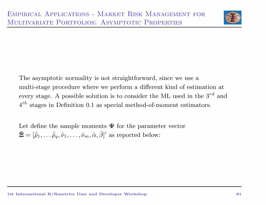
The asymptotic normality is not straightforward, since we use a
multi-stage procedure where we perform a different kind of estimation at
every stage. A possible solution is to consider the ML used in the 3rd and
4th stages in Definition 0.1 as special method-of-moment estimators.
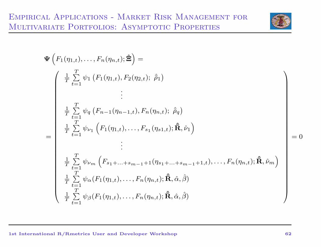
Let define the sample moments Ψ for the parameter vector
Ξ = [ˆρ1, . . . ˆρq, ν1, . . . , νm, α, β]′ as reported below:
1st International R/Rmetrics User and Developer Workshop 61
Empirical Applications - Market Risk Management for
Multivariate Portfolios: Asymptotic Properties
Ψ(
F1(η1,t), . . . , Fn(ηn,t); Ξ)
=
=
1T
T∑
t=1ψ1
(
F1(η1,t), F2(η2,t); ˆρ1)
...
1T
T∑
t=1ψq(
Fn−1(ηn−1,t), Fn(ηn,t); ˆρq)
1T
T∑
t=1ψν1
(
F1(η1,t), . . . , Fs1 (ηs1,t);ˆR, ν1
)
..
.
1T
T∑
t=1ψνm
(
Fs1+...+sm−1+1(ηs1+...+sm−1+1,t), . . . , Fn(ηn,t);ˆR, νm
)
1T
T∑
t=1ψα(F1(η1,t), . . . , Fn(ηn,t);
ˆR, α, β)
1T
T∑
t=1ψβ(F1(η1,t), . . . , Fn(ηn,t);
ˆR, α, β)
= 0
1st International R/Rmetrics User and Developer Workshop 62
Empirical Applications - Market Risk Management for
Multivariate Portfolios: Asymptotic Properties
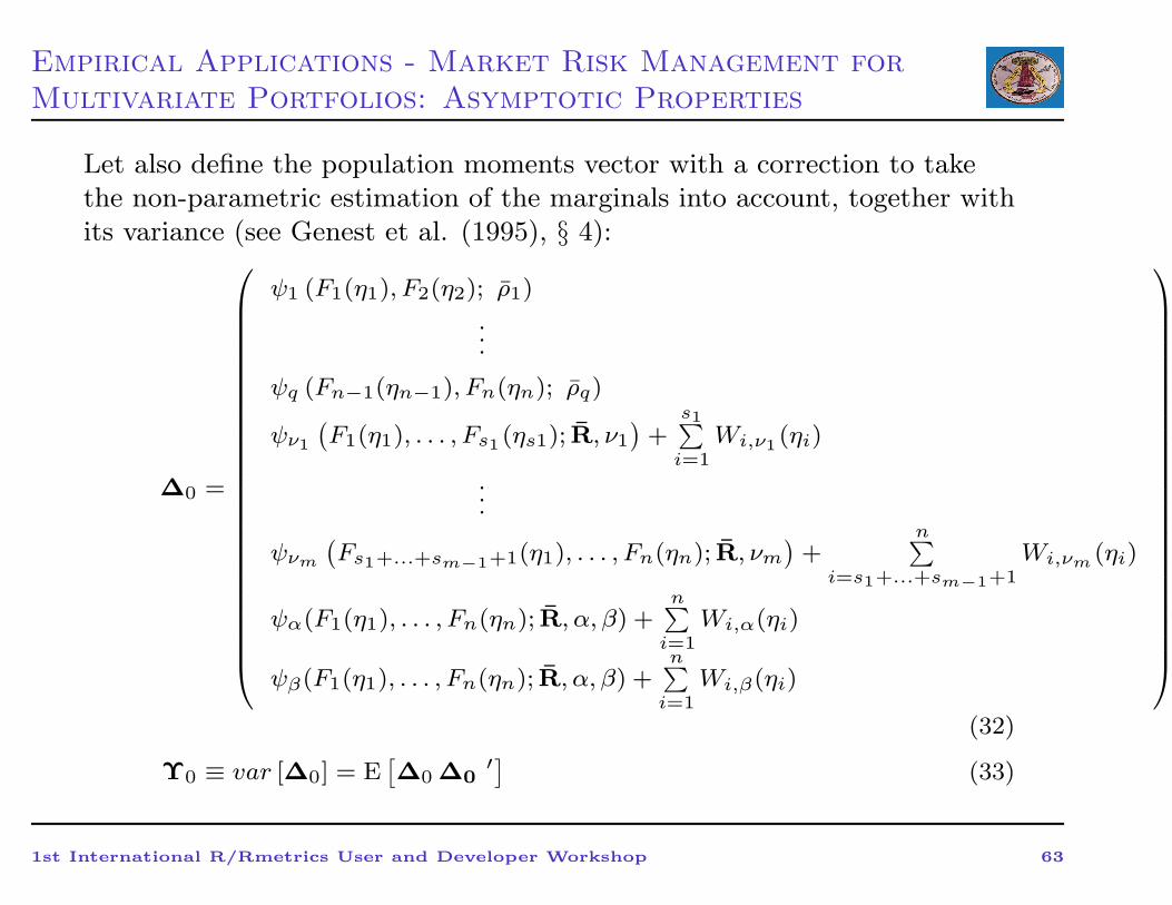
Let also define the population moments vector with a correction to takethe non-parametric estimation of the marginals into account, together withits variance (see Genest et al. (1995), § 4):
∆0 =
ψ1 (F1(η1), F2(η2); ρ1)
.
..
ψq (Fn−1(ηn−1), Fn(ηn); ρq)
ψν1
(
F1(η1), . . . , Fs1 (ηs1); R, ν1)
+s1∑
i=1Wi,ν1 (ηi)
...
ψνm
(
Fs1+...+sm−1+1(η1), . . . , Fn(ηn); R, νm)
+n∑
i=s1+...+sm−1+1Wi,νm (ηi)
ψα(F1(η1), . . . , Fn(ηn); R, α, β) +n∑
i=1Wi,α(ηi)
ψβ(F1(η1), . . . , Fn(ηn); R, α, β) +n∑
i=1Wi,β(ηi)
(32)
Υ0 ≡ var [∆0] = E[
∆0 ∆0′] (33)
1st International R/Rmetrics User and Developer Workshop 63
Empirical Applications - Market Risk Management for
Multivariate Portfolios: Asymptotic Properties
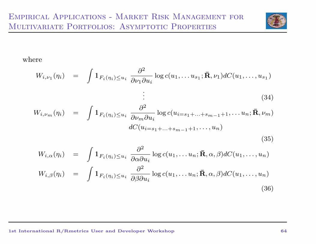
where
Wi,ν1 (ηi) =
∫
1l Fi(ηi)≤ui
∂2
∂ν1∂uilog c(u1, . . . us1 ; R, ν1)dC(u1, . . . , us1 )
... (34)
Wi,νm (ηi) =
∫
1l Fi(ηi)≤ui
∂2
∂νm∂uilog c(ui=s1+...+sm−1+1, . . . un; R, νm)
dC(ui=s1+...+sm−1+1, . . . , un)
(35)
Wi,α(ηi) =
∫
1l Fi(ηi)≤ui
∂2
∂α∂uilog c(u1, . . . un; R, α, β)dC(u1, . . . , un)
Wi,β(ηi) =
∫
1l Fi(ηi)≤ui
∂2
∂β∂uilog c(u1, . . . un; R, α, β)dC(u1, . . . , un)
(36)
1st International R/Rmetrics User and Developer Workshop 64
Empirical Applications - Market Risk Management for
Multivariate Portfolios: Asymptotic Properties
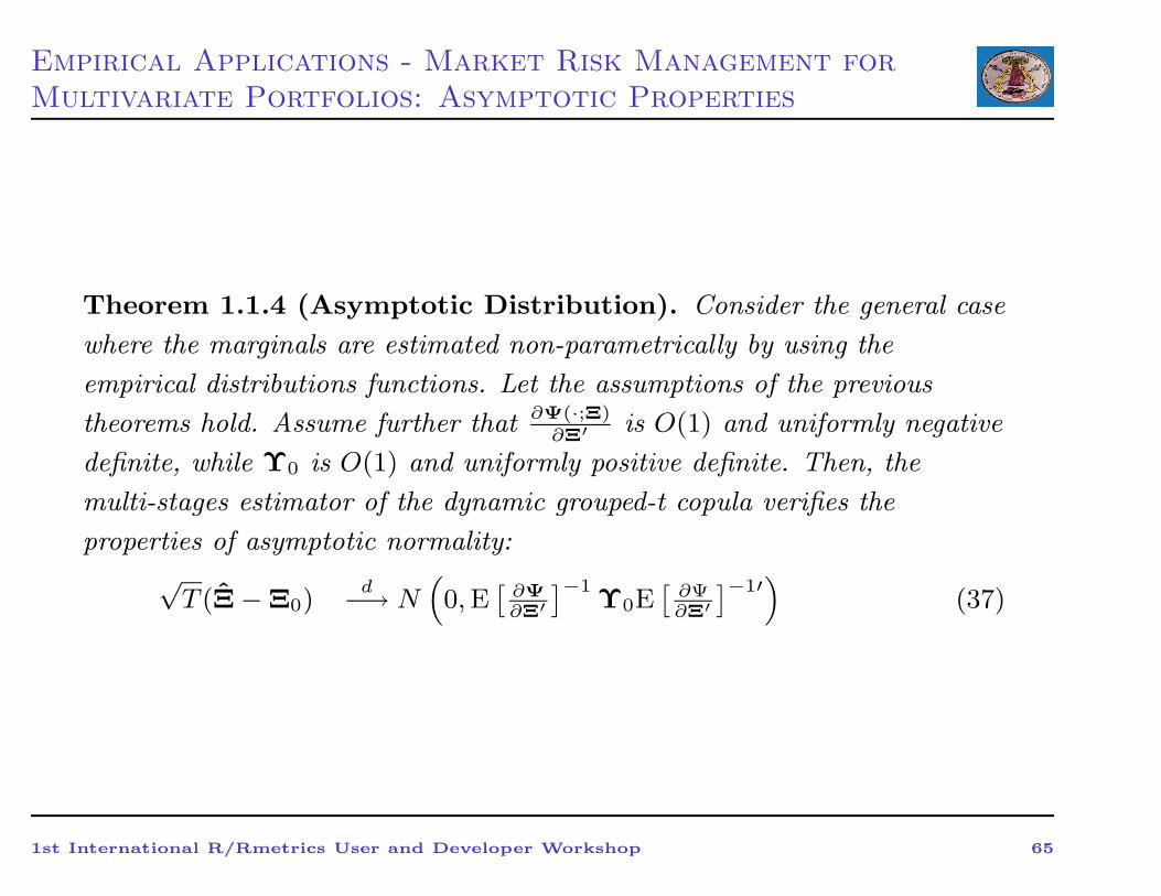
Theorem 1.1.4 (Asymptotic Distribution). Consider the general case
where the marginals are estimated non-parametrically by using the
empirical distributions functions. Let the assumptions of the previous
theorems hold. Assume further that ∂Ψ(·;Ξ)∂Ξ′ is O(1) and uniformly negative
definite, while Υ0 is O(1) and uniformly positive definite. Then, the
multi-stages estimator of the dynamic grouped-t copula verifies the
properties of asymptotic normality:√T (Ξ − Ξ0)
d−→ N(
0,E[
∂Ψ∂Ξ′
]−1Υ0E
[
∂Ψ∂Ξ′
]−1′)
(37)
1st International R/Rmetrics User and Developer Workshop 65
Empirical Applications - Market Risk Management for
Multivariate Portfolios: Simulation Study
The previous asymptotic properties hold only under the very special case
when zi, zj are uncorrelated and R is the identity matrix. When this
restriction does not hold, the estimation procedure previously described
may not deliver consistent estimates.
Daul et al. (2003) performed a Monte-Carlo study with a grouped-t copula
with constant R, employing an estimation procedure equal to the first
three steps of definition 0.1.
They showed that the correlations parameters present a bias that increases
nonlinearly in Rj,k, but the magnitude of the error is rather low. Instead,
no evidence is reported for the degrees of freedom.
1st International R/Rmetrics User and Developer Workshop 66
Empirical Applications - Market Risk Management for
Multivariate Portfolios: Simulation Study
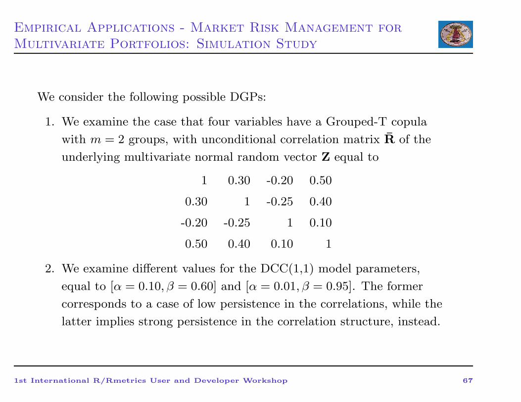
We consider the following possible DGPs:
1. We examine the case that four variables have a Grouped-T copula
with m = 2 groups, with unconditional correlation matrix R of the
underlying multivariate normal random vector Z equal to
1 0.30 -0.20 0.50
0.30 1 -0.25 0.40
-0.20 -0.25 1 0.10
0.50 0.40 0.10 1
2. We examine different values for the DCC(1,1) model parameters,
equal to [α = 0.10, β = 0.60] and [α = 0.01, β = 0.95]. The former
corresponds to a case of low persistence in the correlations, while the
latter implies strong persistence in the correlation structure, instead.
1st International R/Rmetrics User and Developer Workshop 67
Empirical Applications - Market Risk Management for
Multivariate Portfolios: Simulation Study
3. We examine two cases for the degrees of freedom νk for the m = 2
groups:
• ν1 = 3 and ν2 = 4;
• ν1 = 6 and ν2 = 15;
The first case corresponds to a situation of strong tail dependence, that
is there is a high probability to observe an extremely large observation
on one variable, given that the other variable has yielded an extremely
large observation. The last exhibit low tail dependence, instead.
4. We consider three possible data situations: n = 500, n = 1000 and
n = 10000.
1st International R/Rmetrics User and Developer Workshop 68
Empirical Applications - Market Risk Management for
Multivariate Portfolios: Simulation Study
• Unconditional correlation parameters Rj,k: there is a general negative
bias that stabilize after n = 1000. However, this bias is quite high
when there is strong tail dependence among variables (νk are low),
while it is much lower when the tail dependence is rather weak (νk are
high). Besides, it almost disappears when correlations are lower than
0.10, thus confirming the previous asymptotics results. The effects of
different dynamic structure in the correlations are negligible, instead.
• DCC(1,1) parameters (α, β): the higher is the persistence in the
correlations structure (high β), the quicker β converges to the true
values. In general, the effects of different DGPs on β are almost
negligible. The parameter α describing the effect of past shocks shows
positive biases, instead, that are higher in magnitude when high tail
dependence and high persistence in the correlations are considered.
1st International R/Rmetrics User and Developer Workshop 69
Empirical Applications - Market Risk Management for
Multivariate Portfolios: Simulation Study
• Degrees of freedom νk: the speed of convergence towards the true
values is, in general, very low and changes substantially according to
the magnitude of νk and the dynamic structure in the correlations.
Particularly, when there is high tail dependence (νk are low) the
convergence is much quicker than when there is low tail dependence
(νk are high). Furthermore, the convergence is quicker when there is
strong persistence in the correlations structure (β is high), rather than
the persistence is weak (β is low).
This is good news since financial assets usually show high tail
dependence and high persistence in the correlations (see Mcneil et al.
(2005) and references therein). Besides, it is interesting to note that
the biases are negative for all the considered DGPs, i.e. the estimated
νk are lower than the true values νk.
1st International R/Rmetrics User and Developer Workshop 70
Empirical Applications - Market Risk Management for
Multivariate Portfolios: Simulation Study
We explore the consequences of our multi-step estimation procedure of the
dynamic grouped-t copula on Value at Risk (VaR) estimation, by using
the same DGPs previously discussed.
As we want to study only the effects of the estimated dependence
structure, we consider the same marginals for all DGPs, as well as the
same past shocks ut−1. For sake of simplicity, we suppose to invest an
amount Mi = 1$, i = 1, . . . , n = 4 in every asset.
We consider eight different quantiles to better highlight the overall effects
of the estimated copula parameters on the joint distribution of the losses:
0.25%, 0.50%, 1.00%, 5.00%, 95.00%, 99.00%, 99.50%, 99.75%.
1st International R/Rmetrics User and Developer Workshop 71
Empirical Applications - Market Risk Management for
Multivariate Portfolios: Simulation Study
In general, the estimated quantiles show a very small underestimation,
which can range between 0 and 3%. Particularly, we can observe that
• the error in the approximation of the quantiles is lower the lower the
tail dependence between assets is, i.e. when νk are high, ceteris
paribus. As a consequence, when estimating the quantile they tend to
offset the effect of lower correlations, which would decrease the
computed quantile, instead.
• the error in the approximation of the quantiles is lower the higher is
the persistence in the correlations, ceteris paribus. This result is due to
the much smaller biases of the parameters α, β when the true DGPs
are characterized by high persistence in the correlations.
1st International R/Rmetrics User and Developer Workshop 72
Empirical Applications - Market Risk Management for
Multivariate Portfolios: Simulation Study
• the error in the approximation of the quantiles tend to slightly increase
as long as the sample dimension increases. Such a result can be
explained considering that the computed degrees of freedom νk slowly
converge to the true values when the dimension of the dataset
increases, while the negative biases in the correlations tend to
stabilize. As a consequence, the computed νk do not offset any more
the effect of lower correlations, and therefore the underestimation in
the VaR increases.
• the approximations of the extreme quantiles are much better than those
of the central quantiles, while the analysis reveals no major difference
between left tail and right tail.
• It is interesting to note that up to medium-sized datasets consisting of
n = 1000 observations, the effects of the biases in the degrees of
freedom and the biases in the correlations tend to offset each other and
the error in approximating the quantile is close to zero.
1st International R/Rmetrics User and Developer Workshop 73
Empirical Applications - Market Risk Management for
Multivariate Portfolios: Empirical Analysis
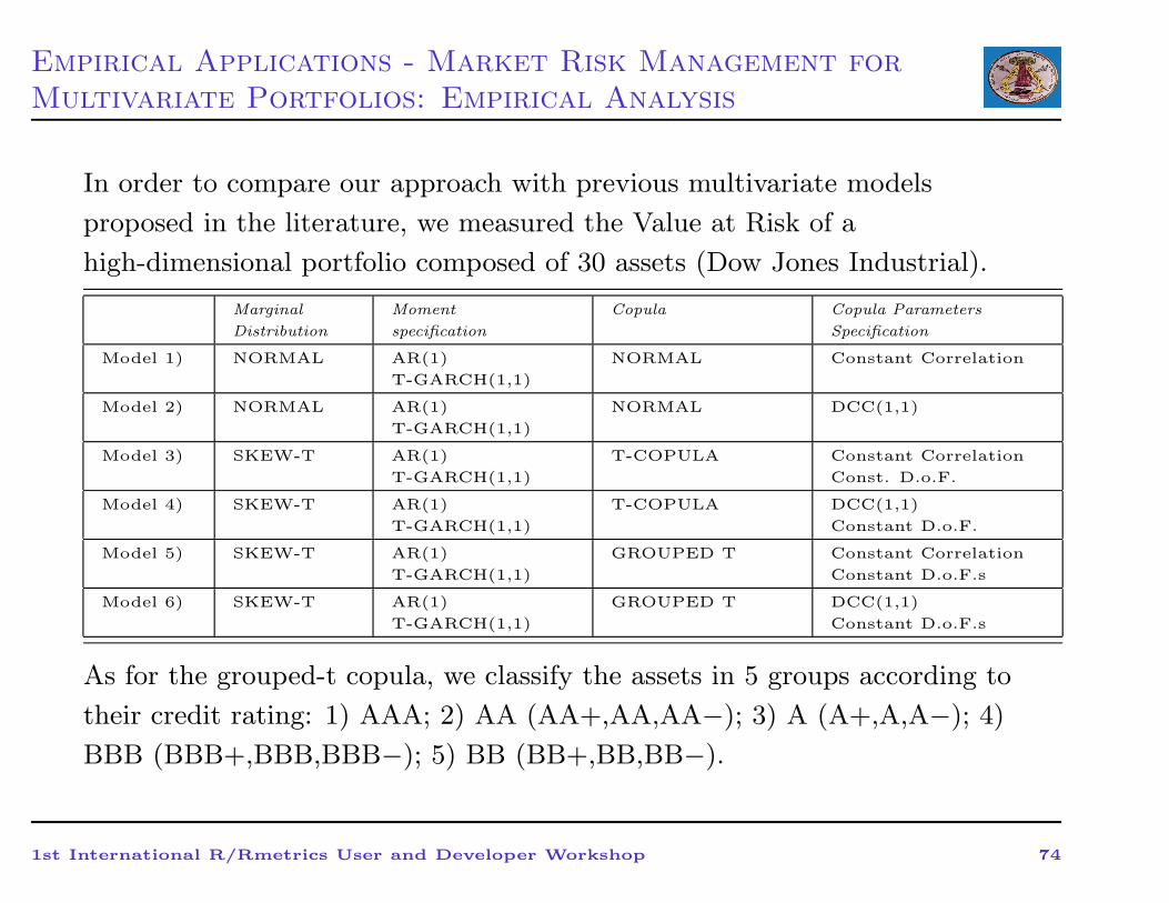
In order to compare our approach with previous multivariate models
proposed in the literature, we measured the Value at Risk of a
high-dimensional portfolio composed of 30 assets (Dow Jones Industrial).
Marginal
Distribution
Moment
specification
Copula Copula Parameters
Specification
Model 1) NORMAL AR(1)
T-GARCH(1,1)
NORMAL Constant Correlation
Model 2) NORMAL AR(1)
T-GARCH(1,1)
NORMAL DCC(1,1)
Model 3) SKEW-T AR(1)
T-GARCH(1,1)
T-COPULA Constant Correlation
Const. D.o.F.
Model 4) SKEW-T AR(1)
T-GARCH(1,1)
T-COPULA DCC(1,1)
Constant D.o.F.
Model 5) SKEW-T AR(1)
T-GARCH(1,1)
GROUPED T Constant Correlation
Constant D.o.F.s
Model 6) SKEW-T AR(1)
T-GARCH(1,1)
GROUPED T DCC(1,1)
Constant D.o.F.s
As for the grouped-t copula, we classify the assets in 5 groups according to
their credit rating: 1) AAA; 2) AA (AA+,AA,AA−); 3) A (A+,A,A−); 4)
BBB (BBB+,BBB,BBB−); 5) BB (BB+,BB,BB−).
1st International R/Rmetrics User and Developer Workshop 74
Empirical Applications - Market Risk Management for
Multivariate Portfolios: Empirical Analysis
We will assess the performance of the competing multivariate models using
the following back-testing techniques
• Kupiec (1995) unconditional coverage test;
• Christoffersen (1998) conditional coverage test;
• Loss functions to evaluate VaR forecast accuracy;
• Hansen and Lunde (2005) and Hansen’s (2005) Superior Predictive
Ability (SPA) test.
1st International R/Rmetrics User and Developer Workshop 75
Empirical Applications - Market Risk Management for
Multivariate Portfolios: Empirical Analysis
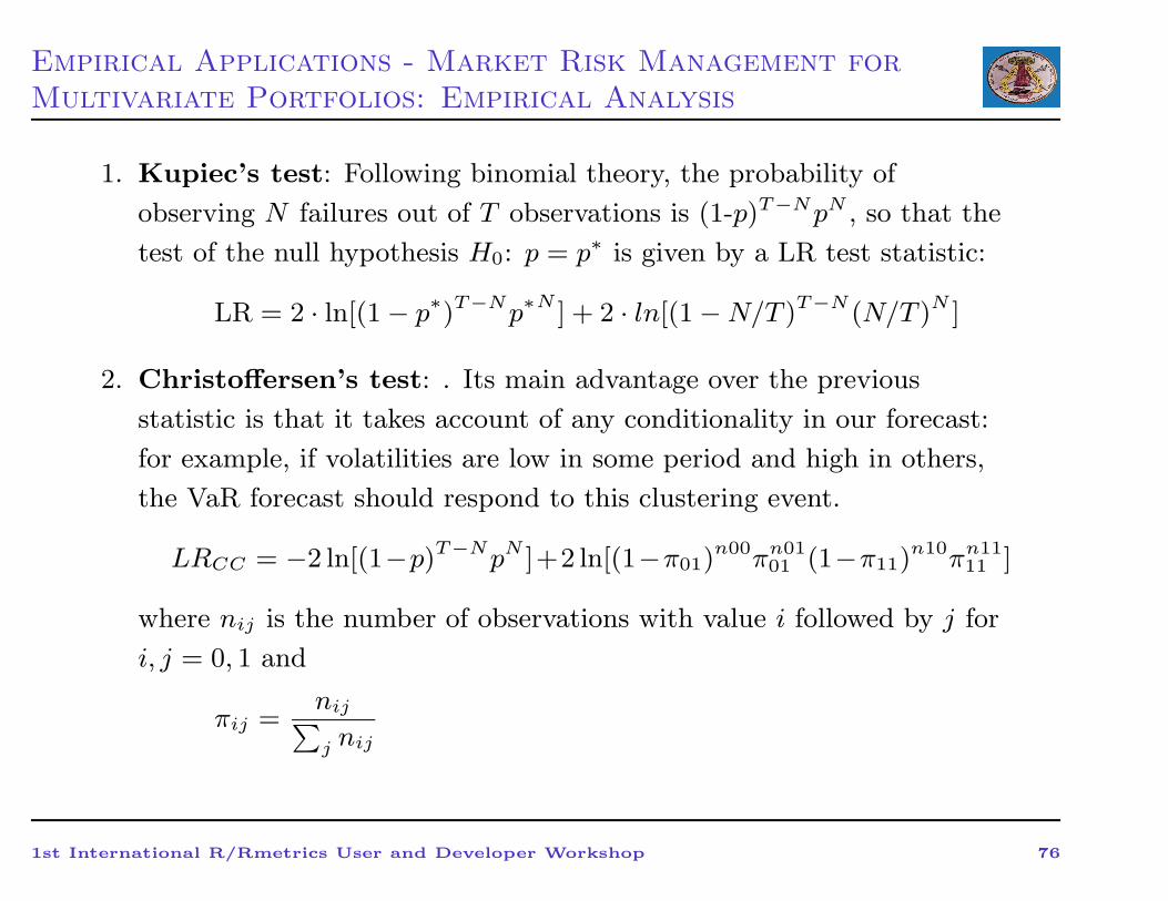
1. Kupiec’s test: Following binomial theory, the probability of
observing N failures out of T observations is (1-p)T−NpN , so that the
test of the null hypothesis H0: p = p∗ is given by a LR test statistic:
LR = 2 · ln[(1 − p∗)T−Np∗N
] + 2 · ln[(1 −N/T )T−N (N/T )N ]
2. Christoffersen’s test: . Its main advantage over the previous
statistic is that it takes account of any conditionality in our forecast:
for example, if volatilities are low in some period and high in others,
the VaR forecast should respond to this clustering event.
LRCC = −2 ln[(1−p)T−NpN ]+2 ln[(1−π01)n00πn01
01 (1−π11)n10πn11
11 ]
where nij is the number of observations with value i followed by j for
i, j = 0, 1 and
πij =nij
∑
j nij
1st International R/Rmetrics User and Developer Workshop 76
Empirical Applications - Market Risk Management for
Multivariate Portfolios: Empirical Analysis
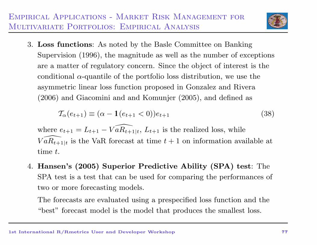
3. Loss functions: As noted by the Basle Committee on Banking
Supervision (1996), the magnitude as well as the number of exceptions
are a matter of regulatory concern. Since the object of interest is the
conditional α-quantile of the portfolio loss distribution, we use the
asymmetric linear loss function proposed in Gonzalez and Rivera
(2006) and Giacomini and and Komunjer (2005), and defined as
Tα(et+1) ≡ (α− 1l (et+1 < 0))et+1 (38)
where et+1 = Lt+1 − V aRt+1|t, Lt+1 is the realized loss, while
V aRt+1|t is the VaR forecast at time t+ 1 on information available at
time t.
4. Hansen’s (2005) Superior Predictive Ability (SPA) test: The
SPA test is a test that can be used for comparing the performances of
two or more forecasting models.
The forecasts are evaluated using a prespecified loss function and the
“best” forecast model is the model that produces the smallest loss.
1st International R/Rmetrics User and Developer Workshop 77
Empirical Applications - Market Risk Management for
Multivariate Portfolios: Empirical Analysis
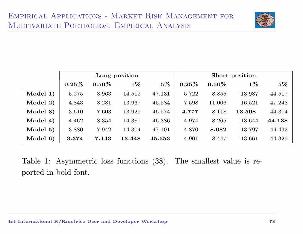
Long position Short position
0.25% 0.50% 1% 5% 0.25% 0.50% 1% 5%
Model 1) 5.275 8.963 14.512 47.131 5.722 8.855 13.987 44.517
Model 2) 4.843 8.281 13.967 45.584 7.598 11.006 16.521 47.243
Model 3) 3.610 7.603 13.929 46.574 4.777 8.118 13.508 44.314
Model 4) 4.462 8.354 14.381 46.386 4.974 8.265 13.644 44.138
Model 5) 3.880 7.942 14.304 47.101 4.870 8.082 13.797 44.432
Model 6) 3.374 7.143 13.448 45.553 4.901 8.447 13.661 44.329
Table 1: Asymmetric loss functions (38). The smallest value is re-
ported in bold font.
1st International R/Rmetrics User and Developer Workshop 78
Empirical Applications - Market Risk Management for
Multivariate Portfolios: Empirical Analysis
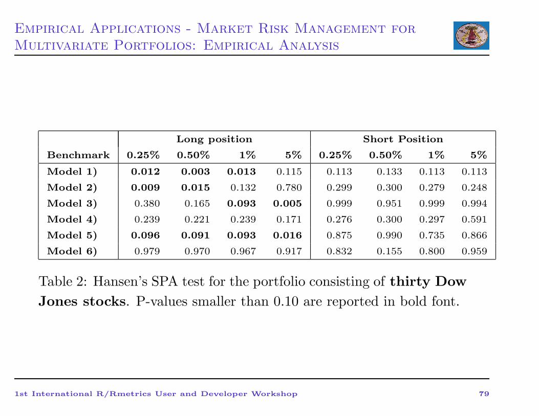
Long position Short Position
Benchmark 0.25% 0.50% 1% 5% 0.25% 0.50% 1% 5%
Model 1) 0.012 0.003 0.013 0.115 0.113 0.133 0.113 0.113
Model 2) 0.009 0.015 0.132 0.780 0.299 0.300 0.279 0.248
Model 3) 0.380 0.165 0.093 0.005 0.999 0.951 0.999 0.994
Model 4) 0.239 0.221 0.239 0.171 0.276 0.300 0.297 0.591
Model 5) 0.096 0.091 0.093 0.016 0.875 0.990 0.735 0.866
Model 6) 0.979 0.970 0.967 0.917 0.832 0.155 0.800 0.959
Table 2: Hansen’s SPA test for the portfolio consisting of thirty Dow
Jones stocks. P-values smaller than 0.10 are reported in bold font.
1st International R/Rmetrics User and Developer Workshop 79
Empirical Applications - Market Risk Management for
Multivariate Portfolios: Empirical Analysis
Long positions
0.25% 0.50% 1% 5%
M. N/T pUC pCC N/T pUC pCC N/T pUC pCC N/T pUC pCC
1) 1.40% 0.00 0.00 1.90% 0.00 0.00 2.30% 0.00 0.00 6.30% 0.07 0.19
2) 1.30% 0.00 0.00 1.60% 0.00 0.00 1.90% 0.01 0.03 5.80% 0.26 0.49
3) 0.90% 0.00 0.01 1.40% 0.00 0.00 2.00% 0.01 0.01 6.60% 0.03 0.08
4) 0.60% 0.06 0.17 1.40% 0.00 0.00 1.90% 0.01 0.03 6.20% 0.09 0.24
5) 0.80% 0.01 0.02 1.30% 0.00 0.00 1.90% 0.01 0.03 6.10% 0.12 0.18
6) 0.50% 0.16 0.37 1.10% 0.02 0.02 1.80% 0.02 0.05 6.00% 0.16 0.35
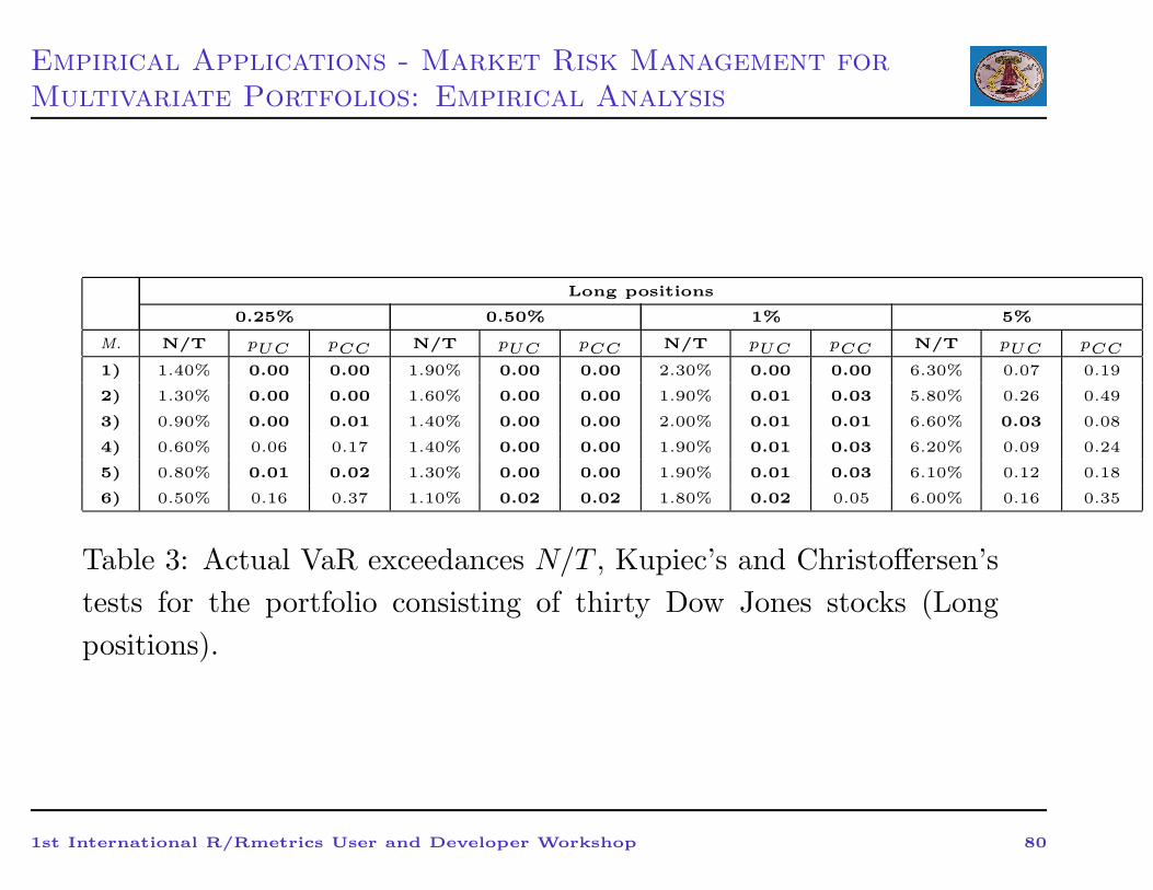
Table 3: Actual VaR exceedances N/T , Kupiec’s and Christoffersen’s
tests for the portfolio consisting of thirty Dow Jones stocks (Long
positions).
1st International R/Rmetrics User and Developer Workshop 80
Empirical Applications - Market Risk Management for
Multivariate Portfolios: Empirical Analysis
Short positions
0.25% 0.50% 1% 5%
M. N/T pUC pCC N/T pUC pCC N/T pUC pCC N/T pUC pCC
1) 0.80% 0.01 0.02 1.00% 0.05 0.06 1.50% 0.14 0.16 5.30% 0.67 0.71
2) 0.70% 0.02 0.06 0.90% 0.11 0.06 1.30% 0.36 0.56 5.00% 1.00 0.95
3) 0.20% 0.74 0.94 0.70% 0.40 0.07 0.90% 0.75 0.87 5.90% 0.20 0.43
4) 0.30% 0.76 0.95 0.70% 0.40 0.06 0.90% 0.75 0.87 5.50% 0.47 0.77
5) 0.30% 0.76 0.95 0.80% 0.22 0.06 0.90% 0.75 0.87 4.80% 0.77 0.54
6) 0.30% 0.76 0.95 0.70% 0.40 0.35 0.90% 0.75 0.87 5.20% 0.77 0.94
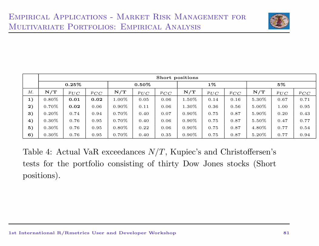
Table 4: Actual VaR exceedances N/T , Kupiec’s and Christoffersen’s
tests for the portfolio consisting of thirty Dow Jones stocks (Short
positions).
1st International R/Rmetrics User and Developer Workshop 81
Empirical Applications - Market Risk Management for
Multivariate Portfolios: Conclusions
• Introduction of the dynamic grouped-t copula for the joint
modelling of high-dimensional portfolios, where we use the DCC
model to specify the time evolution of the correlation matrix of
the grouped-t copula.
• Consistency and asymptotic normality of the estimator under the
special case of a correlation matrix equal to the identity matrix.
• Monte Carlo simulations to study the properties of this estimator
under different data generating processes where such a strong
restriction on the correlation matrix does not hold.
• We investigated the effects of such biases and finite sample
properties on conditional quantile estimation, given the
increasing importance of the Value-at-Risk as risk measure. We
found that the error in the approximation of the quantile can
range between 0 and 3%.
1st International R/Rmetrics User and Developer Workshop 82
Empirical Applications - Market Risk Management for
Multivariate Portfolios: Conclusions
• Empirical analysis 1: When long positions were of concern, we
found that the dynamic grouped-T copula (together with
skewed-t marginals) outperformed both the constant grouped-t
copula and the dynamic student’s T copula as well as the
dynamic multivariate normal model proposed in Engle (2002).
• Empirical analysis 2: As for short positions, we found out that a
multivariate normal model with dynamic normal marginals and
constant normal copula was already a proper choice. This last
result confirms previous evidence in Junker and May (2005) and
Fantazzini (2007) for bivariate portfolios.
• Avenue for future research 1: more sophisticated methods to
separate the assets into homogenous groups when using the
grouped-t copula.
• Avenue for future research 2: look for alternatives to DCC
modelling
1st International R/Rmetrics User and Developer Workshop 83
C-VaR and VaR for Portfolio Management
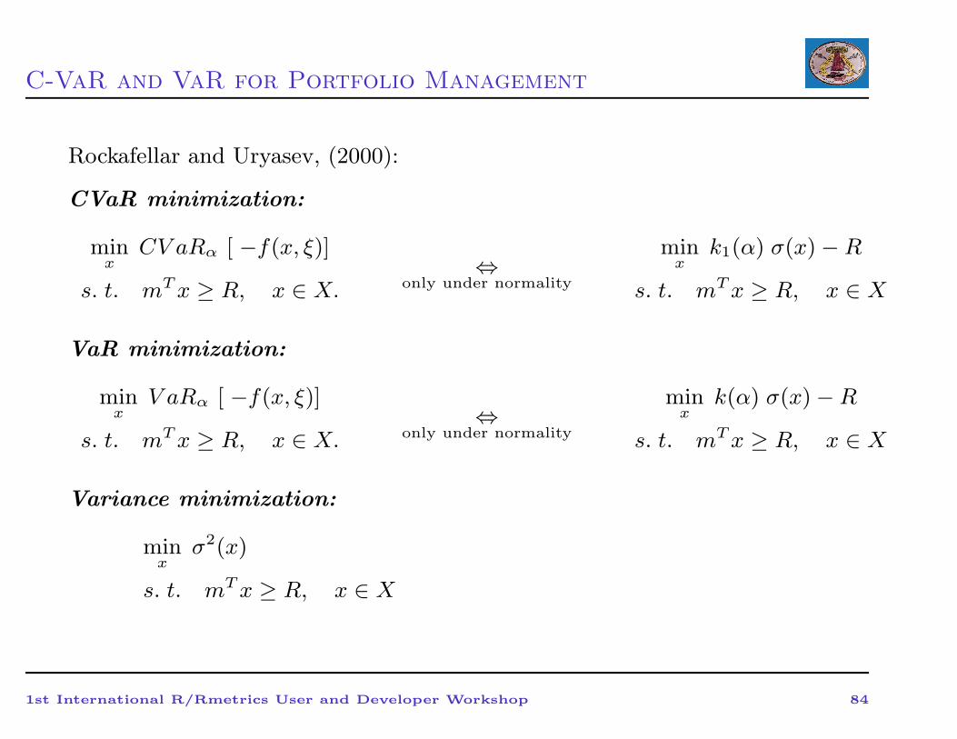
Rockafellar and Uryasev, (2000):
CVaR minimization:
minx
CV aRα [ −f(x, ξ)]
s. t. mTx ≥ R, x ∈ X.⇔
only under normality
minx
k1(α) σ(x) −R
s. t. mTx ≥ R, x ∈ X
VaR minimization:
minx
V aRα [ −f(x, ξ)]
s. t. mTx ≥ R, x ∈ X.⇔
only under normality
minx
k(α) σ(x) −R
s. t. mTx ≥ R, x ∈ X
Variance minimization:
minx
σ2(x)
s. t. mTx ≥ R, x ∈ X
1st International R/Rmetrics User and Developer Workshop 84
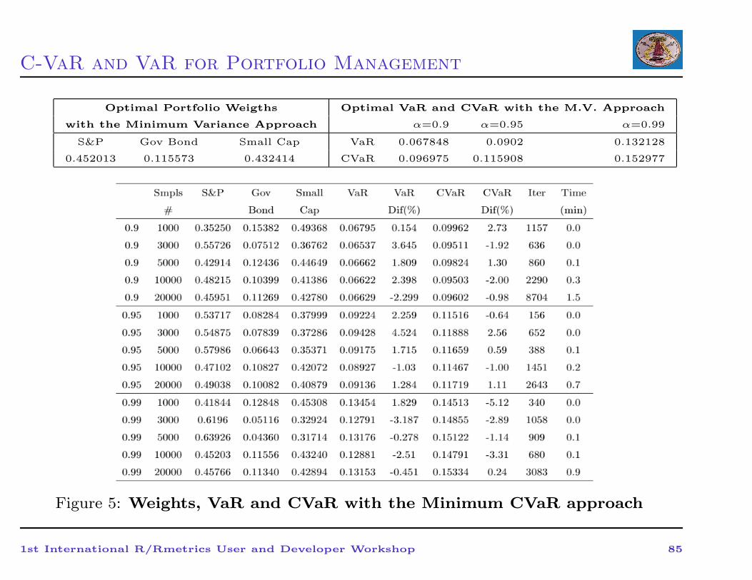
C-VaR and VaR for Portfolio Management
Optimal Portfolio Weigths Optimal VaR and CVaR with the M.V. Approach
with the Minimum Variance Approach α=0.9 α=0.95 α=0.99
S&P Gov Bond Small Cap VaR 0.067848 0.0902 0.132128
0.452013 0.115573 0.432414 CVaR 0.096975 0.115908 0.152977
Figure 5: Weights, VaR and CVaR with the Minimum CVaR approach
1st International R/Rmetrics User and Developer Workshop 85
C-VaR and VaR for Portfolio Management
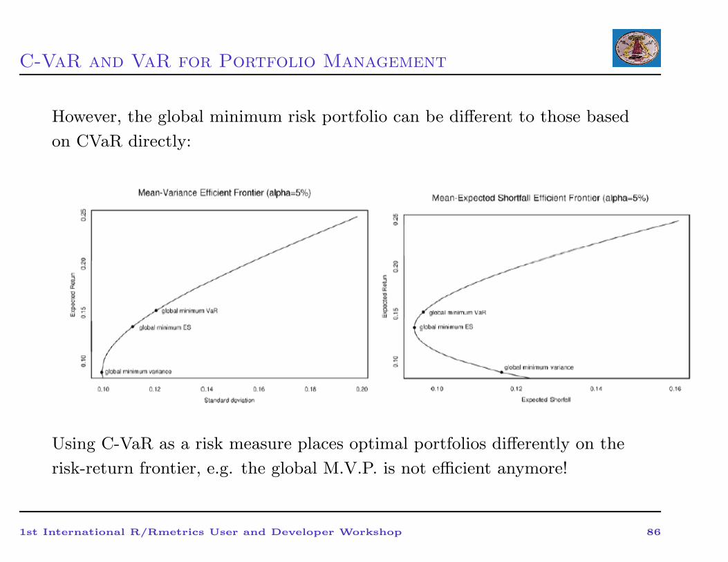
However, the global minimum risk portfolio can be different to those based
on CVaR directly:
Using C-VaR as a risk measure places optimal portfolios differently on the
risk-return frontier, e.g. the global M.V.P. is not efficient anymore!
1st International R/Rmetrics User and Developer Workshop 86