1

RHINO 2.0 Reference Manual (partners User’s Guide)

2

RHINO 2.0 Reference Manual (partners User’s Guide).................................................................1

WHAT’S NEW IN RHINO 2.0 ......................................................................................................................................... 5 INTRODUCTION................................................................................................................................................................. 8

1. What type of data can RHINO analyse ? ........................................................................................................ 8 2. Basic principles behind Mark-Recapture techniques ................................................................................ 11 3. Why getting an estimate of true population size is better than a minimum index ....................... 12 4. What led to the original development of RHINO in 1991 .......................................................................... 12 5. RHINO and violations of classical Mark-Recapture assumptions....................................................... 12 6. RHINO — Ease of use versus Abuse of Statistics .................................................................................... 13 7. RHINO — A Bayesian technique........................................................................................................................ 14 8. RHINO — How well has it worked in practice? .............................................................................................. 15

8.1 Pilanesberg National Park ......................................................................................................................... 15 8.2 Ithala Game Reserve.................................................................................................................................. 15 8.3 Hluhluwe-Imfolozi Park ...............................................................................................................................16 8.4 Mkhuze Game Reserve...............................................................................................................................18 8.5 Ol Pejeta and Ol Jogi.................................................................................................................................18 8.6 Final comments ...........................................................................................................................................18

METHODS........................................................................................................................................................................20 1. Breakdown of a population into segments...................................................................................................20 2. Population Estimation of Identifiable (ID) Independents........................................................................ 21

2.1 The basic "Underhill" Bayesian mark-recapture algorithm used by RHINO .............................. 21 2.2 Dealing with violations of basic "Underhill" method assumptions..............................................23 2.3 Independent Identifiable Priors ..............................................................................................................24

2.3.1 Uninformative Priors ..........................................................................................................................24 2.3.2 Informative Priors ..............................................................................................................................25 2.3.3 Previously saved Priors................................................................................................................... 26 2.3.4 New checks for unrealistic Priors ................................................................................................. 27

2.4 Least squares fitting of truncated Poisson distributions against observed sighting frequencies as an aid to determining the number of sightings/animal allowable before treating individuals as trap-happy .................................................................................................................................28 2.5 Trap-happy animal identification and problems caused by area-happy sampling...............32

2.5.1 RHINO 1.21 - Area-happy sub-sampling ......................................................................................32 2.5.2 RHINO 2..0 - Multi-area analysis.................................................................................................32 2.5.3 Problems caused when discrete survey data are combined with standard "one-at-a-time" observations .........................................................................................................................................32

2.6 Special code datasets - Dealing with violations of the closure assumption..........................32 2.6.1 Special codes .......................................................................................................................................32 2.6.2 Dealing with incomplete independent mortality records......................................................34

3

2.7 Getting population estimates, credible posterior intervals, and measures of skewness and peakedness from the posterior ID independent probability distribution. ................................35

2.7.1 Population estimates .......................................................................................................................35 2.7.2 Credible Posterior Intervals ............................................................................................................35 2.7.3 Measure of Skewness ..................................................................................................................... 36 2.7.4 Measure of Peakedness ..................................................................................................................37

2.8 Effect of small sample biases on ID independent estimates .......................................................37 2.9 Multi-Area analysis ................................................................................................................................... 38

2.9.1 Defining multi-areas.......................................................................................................................... 38 2.9.2 Problems caused by cross-boundary movement of animals .............................................. 38 2.9.3 Sightings Cross-tabulation ......................................................................................................... 39 2.9.4 Allocation of cross boundary sightings for analysis purposes........................................ 39 2.9.5 Cross-boundary movement correction factor (Xboundary CF) ........................................ 39 2.9.6 Initial Analysis-Area population estimation ............................................................................ 40 2.9.7 Using the XboundaryCF to bias-correct mean population estimates .............................. 40 2.9.8 Calculation of bias-corrected mode and median population estimates and bias corrected CPI's ............................................................................................................................................... 40 2.9.9 Uncorrected estimates ................................................................................................................... 40 2.9.10 Calculation of total Park ID Independent Population Estimates and CPI's................ 40

3. POPULATION ESTIMATION OF CLEAN INDEPENDENTS.........................................................................41 3.1 Assumptions ...................................................................................................................................................41 3.2 Basic approach for estimating the number of clean independents.............................................41

3.2.1 Stage 1 : Derivation of the Weighting Function......................................................................42 3.2.2. Stage 2 : Estimation of the distribution of Clean Observation Number..................43 3.2.3 Stage 3 : Estimation of the Clean population probability distribution ....................43 3.2.4 Stage 4 : Incorporation of prior knowledge to refine final distribution.....................44 3.2.5 Stage 5 : Calculation of summary statistics ...................................................................44

3.3 Estimating the number of clean independents when there are special codes........................45 3.3.1 Stage 1 : Derivation of the weighting function.........................................................................45 3.3.2 Stage 2 : Estimation of the distribution of Clean Observation Number.................. 47 3.3.3 Stage 3 : Estimation of the Clean population probability distribution .................... 47 3.3.4 Stage 4 : Incorporation of prior knowledge to refine final distribution.................... 48 3.3.5 Stage 5 : Calculation of summary statistics .................................................................. 48

3.4 Multi-Area Analysis Clean Independent Calculations .................................................................... 48 3.4.1 Initial Analysis-Area population estimation .............................................................................. 48 3.4.2 Using the XboundaryCF to bias-correct mean population estimates.............................. 48 3.4.3 Calculation of bias-corrected mode and median population estimates and bias corrected CPI's ................................................................................................................................................49 3.4.4. Uncorrected estimates ...................................................................................................................49 3.4.5 Calculation of total Park Clean Independent Population Estimates and CPI's ............49

4. Combining the ID and clean independent distributions to estimate total independent number....................................................................................................................................................................................... 50 4.1 Normal analysis................................................................................................................................................ 50

4

4.2 Multi-area analysis .....................................................................................................................................51 5. ESTIMATION OF THE NUMBER OF DEPENDENTS....................................................................................51

5.1 Making up of Dependent number data set(s) prior to Bootstrapping ........................................51 5.2 Bootstrapping the calf number datasets ..........................................................................................51 5.3 Adjustment of the Bootstrapped distribution.................................................................................53 5.4 Estimation of dependent number during a Multi-Area analysis .................................................54

6. TOTAL POPULATION ESTIMATION ................................................................................................................54 6.1 Straight analysis ........................................................................................................................................54 6.2 Multi-Area analysis ....................................................................................................................................55

Some performance characteristics of RHINO 2.0.............................................................................................55 1 Influence of mark-recapture sampling variability and estimation bias on clean estimation. .....55 2 Influence of binomial sampling error in sampling the proportion of total independent observations which are clean. ..............................................................................................................................55 3 Influence of sample size on clean and ID independent estimator bias and precison ...................55 4 Estimated best measure based on multiple simulations and estimated sample size. .............. 57 5 Influence of the proportion of the independent population that is identifiable on total independent estimator bias and precison ...................................................................................................... 58 6 Influence of the population size on the precision of total independent population size............60 7 Summary of the main performance characteristics of RHINO 2..0 ..................................................60

ACKNOWLEDGEMENTS...............................................................................................................................................61 1 Development of the earlier versions of RHINO ..............................................................................................61 2 Development of RHINO 2.0................................................................................................................................ 62 3. Last but not least ............................................................................................................................................. 64

GLOSSARY OF UNFAMILIAR TERMS OR TERMS USED IN A SPECIFIC WAY BY RHINO ....................67 Clean .............................................................................................................................................................................67 Marked .........................................................................................................................................................................67 Section and Area ....................................................................................................................................................68 Independents and Dependents ...........................................................................................................................68 Non—Active records and Special codes..........................................................................................................68 Active records..........................................................................................................................................................68 Bias.............................................................................................................................................................................. 69 Precision ..................................................................................................................................................................... 69

5

WHAT’S NEW IN RHINO 2.0 RHINO 2.0 has been re-written from scratch and is computationally more efficient than RHINO 1.21. It has been designed to be as easy as possible to use and and has a familiar Windows interface, an electronic on-line user and reference manuals, context sensitive help screens and Camtasia AVI help/training videos. RHINO 2.0 has improved trap-happy animal identification, better graphics, improved reporting, greatly enhanced simulation options and includes a new Multi-area analysis option. Its built in statistical expert system advises users on the best measure to use, how to improve precision around estimates , as well as identify and warn users if results are likely to be unusable/very inaccurate (due to insufficient sightings) or where there are signs that inappropriate prior information has been supplied by the user. The following lists some of the main enhancements in RHINO 2.0 and the main differences with RHINO 1.2 1:

• To use RHINO 2.0 users require either Microsoft Access 97, 2000 or 2003. Reporting currently also requires the user to have Microsoft Word and Microsoft Excel 2000 installed.

• RHINO 2.0’s new Windows style interface will be very familiar to users, hopefully making the software

intuitive and easy to use. RHINO 2.0 now groups related topics together on forms. • Data can be imported into RHINO 2.0 from either Microsoft Access (both tables and results of queries),

Microsoft Excel, or Comma or Tab delimited Text Files. Files/Tables/Queries can now be selected by browsing. For backwards compatibility, RHINO 1.21 format input files can be imported from either Paradox, dBase or FoxPro files

• RHINO 2.0 compatible input files should soon be able to be automatically generated by both SADC

Rhino Programme’s WILDb and Kifaru (Kenyan) rhino databases. Data can also now be imported into RHINO 2.0 from Ezemevelo-KZN-Wildlife’s Animal Population Database simply by calling up the results of an Access query. The greater automation of data input file creation will save users considerable time.

• RHINO 2.0 now comes bundled with electronic user and reference .pdf manuals which are accessible

from the main menu. • To make the software easier to learn and master; and to help reduce the need for expensive training

courses (the value of which can be lost as a result of staff turnover), RHINO 2.0 now comes bundled with the Camtasia AVI player, and a number of context sensitive Camtasia AVI training videos. These can be accessed directly during an analysis by simply clicking on the video icon button whenever it appears on a form.

• Context sensitive text help is also available for most forms by clicking on the help icon button on

forms. The help text can be printed out by the user if desired.

• Unlike previous versions of RHINO, users can now go backwards during an analysis if they would like to change any parameters they have selected. This is a big improvement on previous versions, when users would have had to quit and start the analysis from scratch.

• RHINO 2.0 now automatically generates a summary table describing the sightings and special events

in the dataset being analysed, broken down by population segment.

• RHINO 2.0 also now comes with an installation routine, making it easier to install than earlier versions.

6

• RHINO 2.0 offers a bigger range of data filters to enable to user to select a specific subset of a bigger database for analysis. Users now have the option of filtering data prior to analysis by any combination of dates, area, section, age, sex, special codes, observer quality code, observer name, type of sighting, character sort field and numeric sort field.

• An improved clean estimator is used in RHINO 2.0. Bias can no longer be introduced by users

specifying unrealistically low maximum clean priors; although the user can supply a suggested maximum clean value, and RHINO 2.0 will then calculate and graph the probability of the population being bigger than this value given the data supplied.

• In contrast to earlier versions of RHINO, when an animal is ear-notched to make it identifiable, the

record of this event is no longer treated as an active observation. It is now more realistically assumed that capture teams searching for animals to mark will not have the time or inclination to accurately record identifiable animals they see during capture and marking operations.

• A consistent approach has been taken to dropping extreme values of N with a very small chance of

occurrence (dropping values of N p < 0.00001). During calculations probability distributions are now routinely normalized (so that probabilities sum to 1).

• An improved routine for estimating dependent number when there are special codes and trap happy

animals has been implemented.

• RHINO 2.0 uses a Root Mean Square (RMS) error minimization routine to automatically find the truncated Poisson mean which best fits the observed frequency distribution of sightings of ID animals present for the whole analysis period. Users can also graphically examine how RMS varies with mean sighting frequency. The suggested best-fit Poisson mean value (or other user supplied value) is then (as before) used to specify the maximum number of sightings users should allow before treating animals as trap happy (for a specified significance level). If users select to drop trap-happy animals, the sighting frequency distribution graph is updated, marking dropped animals in red (as opposed to blue), and indicating on the form the number of animals and sightings that will be dropped from the mark-recapture analysis.

• Users can enter uninformative, informative or previously saved priors. Users have the option of

saving both uninformative and informative priors. Thumbnail graphs of saved prior distributions now are included as part of the select saved priors menu. As maximizing the entropy of supplied priors made little difference to the results in RHINO 1.21, this option has been dropped from RHINO 2.0.

• The graphs in RHINO 2.0 have been improved. On all final posterior probability distribution graphs, the

axes of the initial default graphs are now scaled automatically so that the graphs concentrate on the range of values of N of most interest. Users can also now interactively…

1) rescale graphs by varying the minimum and maximum X-axis and maximum Y axis values; 2) chose to view partial ID independent distributions calculated after each fifth of the dataset (only if the minimum ID independent prior was set at 1); 3) examine the effect changing the Credible Posterior Interval (CPI) value on the CPI values (Bayesian equivalent of confidence levels); and/or 4) chose whether to shade CPI (confidence) levels on posterior probability graphs.

• RHINO 2.0’s in-built statistical advisor now checks to see if users may have supplied an unrealistically

low upper ID independent prior value, and will warn users if it detects that there is a high chance that upper priors have been set too low, and there is a high chance that the ID independent population size is larger than the initial maximum prior supplied.

• Separate dependent distributions are generated for calves of both identifiable and clean animals (if

both categories exist), and the total dependent distribution is then automatically generated and

7

displayed as the default dependent graph. All three dependent distributions are now included together on a single form, and different graphs and statistics can be selected using tabs.

• The new RHINO 2.0 includes greatly improved reporting with colour graphs and tables automatically

being inserted into the final reports, which are in the form of an MS Word document. If you interactively re-scale a graph during analysis, the final version shown on the screen is the version that will be used in the report. Currently, reporting requires the user to have Word and Excel installed.

• Greatly improved simulation options have been added to RHINO 2.0. These allow 1) the simulation of

a more complicated single run dataset which now can also include special codes, dependents, and trap happy animals; 2) the multiple simulation and automated summary analysis of large numbers of runs for a given set of paramusereters (which can be used to more objectively determine the cost:benefits of notching different numbers of animals as opposed to collecting more data, as well as providing better guidelines on the minimum proportion of a population of a given size one should aim to have notched, and 3) the simulation of a simple multi-area dataset (to assist with teaching the software).

• RHINO 2.0’s in-built statistical advisor expert system has been improved and is based on the results of

many more simulations (65,000 compared to 635 in RHINO1.21). RHINO 1.21’s statistical advisor simply determined the likely best measure to use for estimating the ID independent population segement and this suggestion was then used for all other segment and total population estimates. RHINO 2.0’s statistical advisor expert system now determines and advises on the likely best measure to use for every single segment and population estimate.

• RHINO 2.0 calculates additional variables (RMS estimated mean sighting number, and calculated

measures of distribution skewness and peakedness), which together with the multiple simulation option, will provide developers with additional data which can be used to improve RHINO’s in-built “statistical expert-system” (which guides and sometimes warns users) in future versions.

• RHINO 2.0 users can now undertake a multi-area analysis to produce separate population estimates

for sub-areas within a large Park. Estimation takes account of the cross-boundary movement of some animals between different sub-areas. The new multi-area analysis with cross-boundary movement correction is a major enhancement to the software and replaces the area weighting in previous versions of RHINO. Crosstabulations of the number of sightings per rhino per area are also generated automatically as part of a multi-area analysis.

• While sound in theory, in practice the area-happy analysis option in RHINO 1.21 often did not work (as

the amount of data analysed was reduced to the level of the area with the lowest sampling effort, often resulting in biased and unreliable estimates. For this reason, and because it significantly increased the complexity if of the calculations, area-happy analysis is no longer offered as an option in RHINO 2.0. RHINO 2.0 users can instead use the new multi-area analysis option if different regions of a large park have different sampling efforts.

• There is a slight difference in the way RHINO 2.0 calculates both the median and Credible Posterior

Intervals (CPI - Bayesian equivalent of confidence levels) from posterior distributions. The median is now the value closest to 0.50 in the cumulative probability distribution (as opposed to the first value where the cumulative probability is >= 0.50). For 90% CPI levels RHINO 2.0 now uses the values of N nearest to cumulative probabilities of 5% and 95% provided the probability is not 0 for the value nearest to 5%, when the next highest value of N will be used. (RHINO 1.21 used the first values with cumulative probalities <=5% and >=95% to derive 90% CPI levels).

8

INTRODUCTION

1. What type of data can RHINO analyse ? RHINO was designed to analyse sighting/resighting data of individual rhino collected on a continual on-going basis. It is not suitable for analyzing sighting data collected from multiple but separate discrete surveys of populations. Although RHINO was specifically designed for use with black rhino; it can be used for any largely solitary non-herding species where a segment of the population is individually recognizable and where sightings are ongoing. Some (but not all) animals in the population need to be recognisable to all observers to use RHINO. It is very important that you understand what sighting data RHINO can use and what it can’t; as well as how to classify sightings into different types for a RHINO analysis.

• RHINO is designed for use with first class sightings from reliable observers. The term first class refers to sightings where all potential obvious identifying features (and in particular both ears) were seen and any ID features/absence of ID features were recorded.

• For analysis purposes first class sightings are classified into Identifiable (ID) or not identifiable to all

observers always (clean).

• Mark-recapture techniques require that every time an ID animal is seen it can be identified as a specific animal. This is why RHINO classifies rhino that can only be identifiable by very subtle/harder to record features or from photos, as clean for the purposes of analysis. A key principle to grasp, is that for an animal to be considered an ID animal by a mark-recapture technique like RHINO, it must always be recognizable as that particular animal every time it is seen properly by any competent trained observer (i.e. pass the ID to all always test). For the purposes of RHINO, ID animals are defined as only those with obvious rather than more subtle/harder to record identifying features.

o For rhinos, the most important features used in individual identification are their ears, as

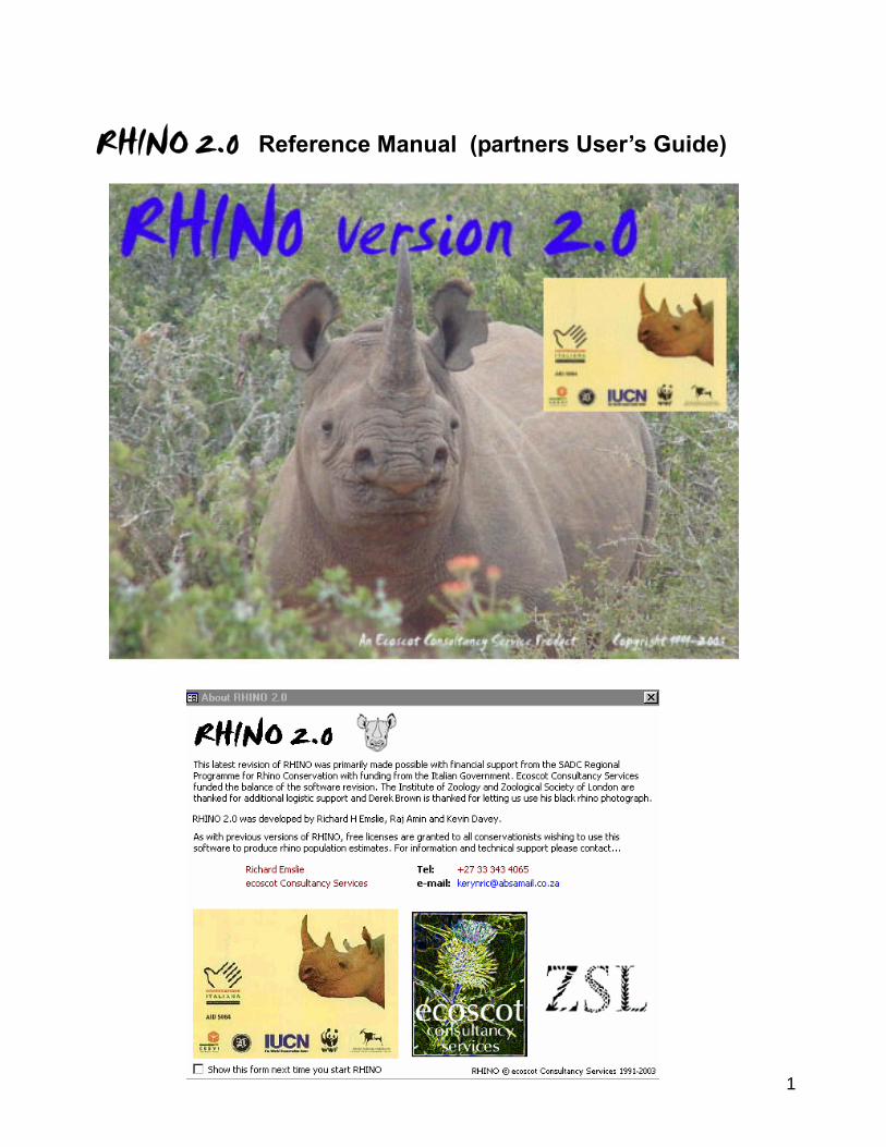
experience has shown that natural ear tears and artificial ear notches can be used to reliably and consistently ID individual rhino by a large number of observers who have been given basic training in rhino ID techniques. The black rhino on RHINO’s opening splash screen is ear-notched and would be clearly identifiable by all trained observers.

o By way of contrast, being able to correctly observe and accurately draw horn configuration

details to scale is a skill that not all observers possess. While digital cameras with a reasonable optical zoom can accurately record such features and the resultant photos can be used to identify individual rhino, not all observers are likely to have digital cameras. Thus in both instances, using horn configurations to ID animals, would fail the ID by all always test. For RHINO analysis purposes, such sightings should be treated as clean sightings (even if in your rhino sightings database the sightings are treated as ID by key observer sightings).

o Rhinos may have even more subtle features (such as their eye wrinkle patterns, minute ear

tears that would be missed by most observers, marks on horns, small scars, etc.) which can allow experienced and highly skilled observers to separate and identify a number of otherwise “clean” animals (especially if photographed). However, when the same animal is seen by other less skilled observers or observers without cameras, it may not be possible to routinely identify it as the same animal. Once again such ID sightings need to be classified as clean sightings.

9

o In the unlikely case where every single observer in a park can accurately record more

subtle/harder to record details (such as horn configurations), and/or all observer teams have digitial cameras, then more subtle/harder to record identification details such as horn configurations could be used to classify sightings as ID for RHINO analysis purposes as in this special case they would pass the ID to all always test.

o RHINO is a Bayesian technique, and so if you have knowledge of the minimum number of

clean rhino identifiable to key observers by more subtle/harder to record features, this information can be incorporated into the analysis and this will ensure that the clean population estimate produced by RHINO will not be less than this known figure.

• Observations from unreliable/untrained observers should not be included in a RHINO analysis. RHINO’s

filtering allows you to easily select to analyse only data from reliable accredited observers.

• To produce the best estimates possible using RHINO it is essential that monitoring does not simply concentrate on identifying as many animals as possible. Equal effort needs to be given to recording first class sightings whether they are of ID or clean animals. In many rhino populations only a fraction of the population is obviously identifiable. When this is the case, to get an accurate estimate of total numbers one needs to accurately estimate what fraction of the population is clean. If one focuses ones attention on ID animals (what has been termed “bubble-gum card collecting”) one will underestimate the proportion of the population of the population that is clean, and produce a biased underestimate of population size.

• Incomplete observations must be excluded from a RHINO analysis. It is very important to appreciate

that an incomplete observation (e.g. where you only saw one of the ears properly before the rhino ran off) is NOT the same as a clean sighting. This mistake has often been made in the past by monitoring programmes when they start up, and are concentrating on identifying as many different rhino as possible. If one incorrectly includes incomplete sightings in the dataset as clean observations , the clean population segment size and total population size will be overestimated.

To recap, to avoid biasing and producing inaccurate population estimates, when undertaking a RHINO analysis 1) only first-class sightings by reliable accredited observers (irrespective of whether the rhino is identifiable or not) should be used, 2) incomplete sightings or sightings by unreliable/untrained observers should be discarded, 3) animals treated as identifiable by RHINO must be able to be identifiable by all observers always, 4) animals identifiable by more subtle/harder to record features should be treated as clean for RHINO purposes and 5) field effort should not be biased in favour of recording ID animals in preference over clean rhino.

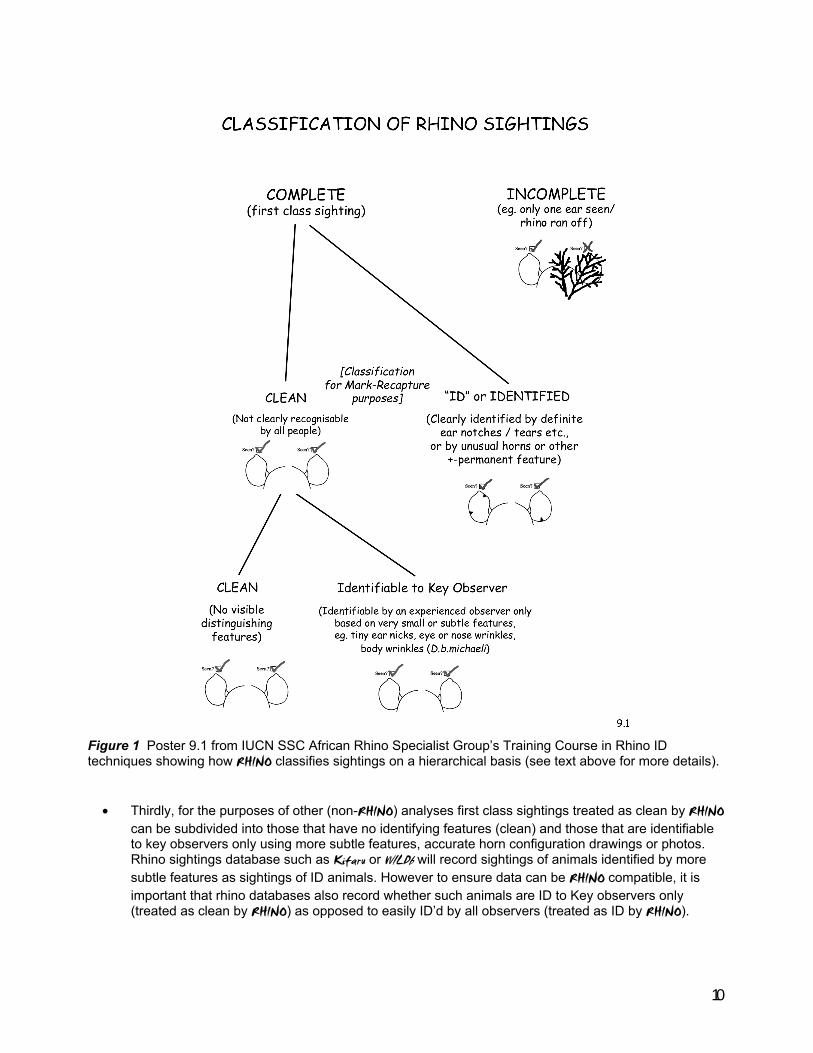
There are three levels of decision when classifying sightings (see Figure 1) .

• Firstly, a decision needs to be made as to whether the sighting is a first class sighting by a reliable observer (and which can be used by RHINO), or whether the sighting was an incomplete sighting or a sighting by an unreliable unaccredited observer (which will not be used by RHINO).

• Secondly, first class sightings are then classified into those which are of obviously identifiable

animals and pass the always by all rule (treated by RHINO as ID sightings), and those which either have no distinguishing feature or which are only identifiable by key observers using more subtle/harder to accurately record features (treated by RHINO as clean sightings).

10

Figure 1 Poster 9.1 from IUCN SSC African Rhino Specialist Group’s Training Course in Rhino ID techniques showing how RHINO classifies sightings on a hierarchical basis (see text above for more details).

• Thirdly, for the purposes of other (non-RHINO) analyses first class sightings treated as clean by RHINO

can be subdivided into those that have no identifying features (clean) and those that are identifiable to key observers only using more subtle features, accurate horn configuration drawings or photos. Rhino sightings database such as Kifaru or WILDb will record sightings of animals identified by more subtle features as sightings of ID animals. However to ensure data can be RHINO compatible, it is important that rhino databases also record whether such animals are ID to Key observers only (treated as clean by RHINO) as opposed to easily ID’d by all observers (treated as ID by RHINO).

11

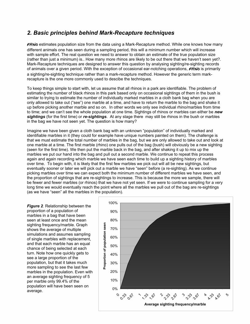
2. Basic principles behind Mark-Recapture techniques RHINO estimates population size from the data using a Mark-Recapture method. While one knows how many different animals one has seen during a sampling period, this will a minimum number which will increase with sample effort. The real question we need to answer to obtain an estimate of the true population size (rather than just a minimum) is.. How many more rhinos are likely to be out there that we haven’t seen yet?. Mark-Recapture techniques are designed to answer this question by analysing sighting/re-sighting records of animals over a given period. With the exception of occasional ear-notching operations, RHINO is primarily a sighting/re-sighting technique rather than a mark-recapture method. However the generic term mark-recapture is the one more commonly used to descibe the techniques. To keep things simple to start with, let us assume that all rhinos in a park are identifiable. The problem of estimating the number of black rhinos in this park based only on occasional sightings of them in the bush is similar to trying to estimate the number of individually marked marbles in a cloth bank bag when you are only allowed to take out (“see”) one marble at a time, and have to return the marble to the bag and shake it up before picking another marble and so on. In other words we only see individual rhino/marbles from time to time; and we can’t see the whole population at one time. Sightings of rhinos or marbles can either be new sightings (for the first time) or re-sightings. At any stage there may still be rhinos in the bush or marbles in the bag we have not seen yet. The question is how many? Imagine we have been given a cloth bank bag with an unknown “population” of individually marked and identifiable marbles in it (they could for example have unique numbers painted on them). The challenge is that we must estimate the total number of marbles in the bag, but we are only allowed to take out and look at one marble at a time. The first marble (rhino) one pulls out of the bag (bush) will obviously be a new sighting (seen for the first time). We then put the marble back in the bag, and after shaking it up to mix up the marbles we put our hand into the bag and pull out a second marble. We continue to repeat this process again and again recording which marble we have seen each time to build up a sighting history of marbles over time. To begin with, it is likely that the first few marbles we pick out will all be new sightings, but eventually sooner or later we will pick out a marble we have “seen” before (a re-sighting). As we continue picking marbles over time we can expect both the minimum number of different marbles we have seen, and the proportion of sightings that are re-sightings to increase. This is because the more we sample, there will be fewer and fewer marbles (or rhinos) that we have not yet seen. If we were to continue sampling for a very long time we would eventually reach the point where all the marbles we pull out of the bag are re-sightings (as we have “seen” all the marbles in the population). Figure 2. Relationship between the proportion of a population of marbles in a bag that have been seen at least once and the mean sighting frequency/marble. Graph shows the average of multiple simulations and assumes sampling of single marbles with replacement, and that each marble has an equal chance of being selected at each turn. Note how one quickly gets to see a large proportion of the population, but that it takes much more sampling to see the last few marbles in the population. Even with an average sighting frequency of 5 per marble only 99.4% of the population will have been seen on average. 0%

10%

20%

30%

40%

50%

60%

70%

80%

90%

100%

00.3

30.6

7 11.3

31.6

7 22.3

32.6

7 33.3

33.6

7 44.3

34.6

7 5

Average sighting frequency/marble

Prop

ortio

n of

pop

ulat

ion

seen

12

Given the sighting/re-sighting history of a population (of rhinos or marbles) it is mathematically possible (using mark-recapture methods) to estimate the probability of the population being each of a range of population sizes. From this information it is possible to derive a population estimate and confidence levels around this estimate. The key principle to grasp here is that as the proportion of “re-sightings” increases one can expect to have seen a higher proportion of the population and hence that there are likely to be fewer rhinos (marbles) left we haven’t seen yet. The corollary is that if by the end of a sampling period we are still getting quite a few new sightings, then it is probable that there are still quite a few rhinos (marbles) in the population we haven’t seen yet. If we have not seen a new rhino (marble) for some time then we can be increasingly confident that we probably have seen all the animals are there are none out there that have not been seen.

3. Why getting an estimate of true population size is better than a minimum index The real advantage of using mark-recapture methods such as RHINO is that one gets a population estimate of the true number of rhinos (marbles) rather than just a count of the number of different animals seen. The latter is just a minimum index, which will increase as we do more sampling. In order to implement a biological management harvesting strategy to prevent overstocking and maintain rapid black rhino population growth (a requirement of all current national and organizational black rhino conservation strategies) managers need estimates of absolute population sizes (not minimum indices). Estimates of the true population size can also be converted to densities, allowing one to compare current densities to recommended maximum productive stocking rates or estimates of ecological carrying capacity for your area.

4. What led to the original development of RHINO in 1991 Unlike the marble example above, in many rhino populations not all individual rhino have features that enable them to be reliably recognised as individuals. In pre-RHINO days (pre-1991) conservation managers on the ground did not have an analytical tool to estimate the number of such clean rhinos in a population. As a result, the focus was very much on how many known ID rhinos there were in the population – what has been termed “bubble-gum card collecting”. Clean sightings were often just lumped with incomplete sightings and largely ignored. As explained above, the problem was that as a result managers were only getting a minimum index of numbers, when estimates of the true population size would be practically far more useful. RHINO was developed specifically to estimate the number of “clean” rhino in the population as well as the probable number of identifiable animals in the population that have not been seen yet. This allowed managers to move beyond “bubble-gum card collecting”, and to analyse both clean and ID sightings data to obtain accurate estimates of total rhino population sizes which practically are of more use.

5. RHINO and violations of classical Mark-Recapture assumptions Mark-recapture techniques have a number of specific assumptions, and if these are violated biased estimates are likely to be produced. In practice, rhino sightings data violate a number of classical mark-recapture assumptions. RHINO was therefore specifically developed to handle as many of these violations of assumptions as possible; and can deal with the following problems…

• Not all rhinos are individually identifiable by all observers always (i.e. some are clean)

13

• Some rhinos are seen very frequently compared to most animals (sighting-happy more commonly referred to in mark-recapture methodology as trap-happy) violating the assumption of approximately equal sightability.

• To collect sufficient data may take a year or two, and during this period the population being studied may change in size over the sampling period; with animals dying, being introduced and/or removed from the population, violating the assumption of closure (i.e the assumption that the population remains the same).

• The proportion of the population that is clean can change during a recording period as a result of management operations to notch (and make identifiable) a number of clean animals

• Sampling effort or sightability may vary in different areas of a reserve (violating the assumption of approximately equal sightability of animals).

• The home range of some rhinos may span two adjacent sub-areas for which you want to obtain separate population estimates. These “cross-boundary” movers will therefore spend less time in specific sub-areas than other resident rhino. This also violates the assumption of approximately equal sightability.

• Sightings of calves seen with their mothers are not statistically independent. Calf (dependent) sightings are therefore excluded from any sighting/resighting calculations. The final population estimate however needs to be adjusted to include dependants.

• Calves grow up and during a sampling period may become independent of their mothers (changing from dependent to independent during a sampling period)

The methods section below gives the details of how RHINO estimates population sizes and deals with the above problems.

6. RHINO – Ease of use versus Abuse of Statistics Many potentially useful statistical techniques end up not being used by field conservationists as they are written in a way that only mathematicians and statisticians can understand them, may only be available in journals not accessible to field biologists, and/or the authors have not packaged their techniques in user-friendly software that can readily be used by field biologists. The developer of RHINO subscribes to the goal formulated in the South African Statistical Association's strategic plan which is: To be accessible to, and supportive of, the users of statistics in the broader community (Zucchini 1992). An active attempt has been made to make the software user-friendly to increase its chance of being routinely applied in the field. The fact that earlier versions of RHINO have been used every year in some parks since 1991 is testament to this. The new RHINO 2 software represents another step forward in user friendliness compared to earlier DOS-based versions of the software. The real danger with easy to use statistical packages is that they can easily be abused by users. It cannot be emphasised enough that any statistical methods need to applied with thought and common sense. While users of RHINO don't need to be concerned with the maths – users need to be aware of the basic principles, key assumptions, and principle factors governing estimate quality. RHINO has been written from the standpoint that the majority of its users will be ecologists and zoologists in the field and not statisticians. While many ecologists often have a strong quantitative background; many zoologists appear to have had very limited statistical training. The developer therefore felt it would be more useful, if the package could instead be modified to help and guide users as much as possible. RHINO versions 1.1 onwards therefore have included a statistical advisor expert system which works in the background and by examining input parameters supplied, the data and the results advises the user. In particular RHINO seeks to detect and flag when the package may be being misused, and to warn the user where gross biases are likely to have been introduced. This philosophy is diametrically opposed to the approach of the early GENSTAT developers who deliberately made the user ask for all output to prevent

14

misuse of statistics (The late Peter Digby personal communication.). While the statistical advisor has been improved in RHINO 2.0 it is hoped to include a greatly enhanced statistical advisor system in future releases of RHINO.

7. RHINO – A Bayesian technique RHINO is a extensive form of Bayesian technique. Bayesian methods don’t just use the data collected to estimate population sizes and confidence levels (as would a standard statistical technique); but also use additional information in the form of user supplied prior probabilities (of the population being different sizes) to start the process. These prior probabilities are then iteratively updated using evidence (the sightings/re-sightings data, and additional information on deaths, removals, markings etc.) to produce final posterior probabilities from which the population estimates are derived. In Bayesian statistics prior knowledge and information (e.g. the minimum number of different clean animals known to exist in the population by key observers using more subtle features and photographs) can be incorporated into the prior probabilities to help inform the analyses. This has the advantage that silly lower confidence levels which are less than the minimum known number can be avoided. Users can either supply uninformative priors or informative priors. The use of prior information is the most controversial aspect of Bayesian methods (Underhill 1989). Bayesian statistics have been criticised on the grounds that different users may obtain different answers by supplying different prior information (Gary White personal communication). However, the developer contends that practically this does not matter, provided Bayesian estimates are on the whole more accurate than those using standard methods. In practice, if you have sufficient sightings data, the results obtained by RHINO using informative or uninformative priors will be very similar and most likely identical. For this reason for most analyses users should select to use simpler uninformative priors. In the past Bayesian statistical methods found little favour in wildlife studies, and for a time there had been almost no investigation of their use with capture-recapture studies (White et al. 1982). This is no longer the case (Castledine 1981, Zucchini & Channing 1986, Gazey & Staley 1986, Underhill 1989, Best & Underhill 1989, Rodrigues et al. 1988, Underhill & Fraser 1989, Hitchins & Emslie unpublished, Emslie 1991, Stead 1991). Bayesian methods have much to offer in many areas of biology, and particularly in estimating parameters of animal populations (Underhill 1989) In wildlife studies the usual way to increase estimate accuracy is to increase sample sizes. Due to logistic difficulties and the high cost of extra surveys and fieldwork this is not always possible (Johnson 1989). Bayesian methods can provide an alternative way to increase accuracy. For example, Bayesian methods have been successfully used to produce more accurate estimates of waterfowl population sizes for most species in most years using aerial count data (Johnson 1989). Similarly the use of Bayesian methods substantially improved estimate precision around the 1985 Umfolozi black rhino population estimate based on sighting:resighting data (Hitchins & Emslie unpublished). As discussed above, Bayesian methods appear to be most appropriate for dealing with small populations. Bayesian methods such as the Zucchini-Channing/Gazey-Staley method have been criticised as computer intensive (Chao 1989). Considering the time it takes to collect black rhino sighting data and the value of the animals concerned, computer time is of little relevance and smacks of "ivory-towerism". From a biologists viewpoint it is far more important that the methods give a decent answer. With the development of cheap personal computing and faster and faster machines computing constraints are no longer the problem they once were and Chao’s criticisms have less relevance today. Another reason advanced for preferring Bayesian methods is that many standard statistical mark-recapture methods are also based on large sample approximations and may be inaccurate for small samples (Zucchini and Channing 1986).

15

8. RHINO – How well has it worked in practice? To date RHINO appears to be a reasonably robust and accurate method when it has been used to estimate numbers in populations that are either known completely, are well known.

8.1 Pilanesberg National Park Based on annual photographic helicopter ID surveys, known introductions and deaths, and because no new animals had been seen for a number of years, the population of 32 black rhino in Pilanesberg National Park was completely known. This gave an ideal opportunity to test out RHINO using data from 4½ months of field ranger sightings. Based solely on the ranger sightings at the end of the monitoring period there were 22 independent rhino and 5 calves giving a minimum of 27. RHINO identified two of the animals as trap-happy, and by chance the final RHINO population estimate of 32 was spot on, with an underestimation of the independent (adult and sub-adult) number by 1 being cancelled out by an overestimate of the number of calves by 1.

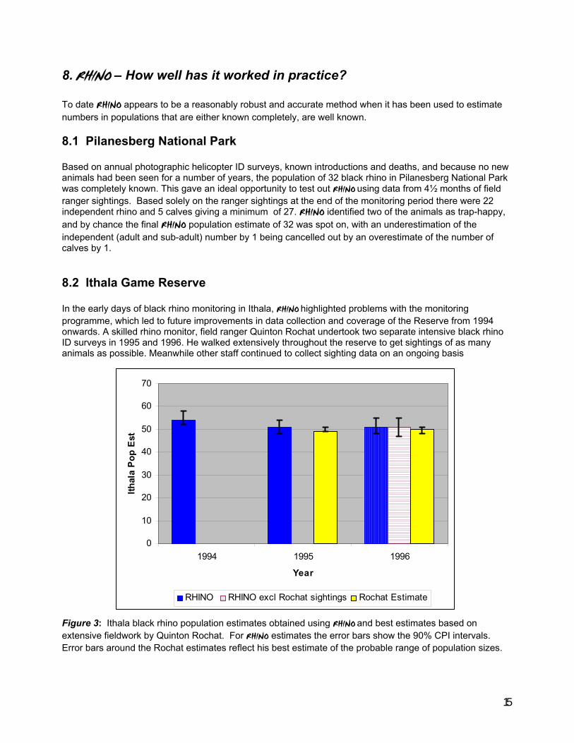
8.2 Ithala Game Reserve In the early days of black rhino monitoring in Ithala, RHINO highlighted problems with the monitoring programme, which led to future improvements in data collection and coverage of the Reserve from 1994 onwards. A skilled rhino monitor, field ranger Quinton Rochat undertook two separate intensive black rhino ID surveys in 1995 and 1996. He walked extensively throughout the reserve to get sightings of as many animals as possible. Meanwhile other staff continued to collect sighting data on an ongoing basis

Figure 3: Ithala black rhino population estimates obtained using RHINO and best estimates based on extensive fieldwork by Quinton Rochat. For RHINO estimates the error bars show the 90% CPI intervals. Error bars around the Rochat estimates reflect his best estimate of the probable range of population sizes.

0

10

20

30

40

50

60

70

1994 1995 1996

Year

Ithal

a Po

p E

st

RHINO RHINO excl Rochat sightings Rochat Estimate

16

In 1996, RHINO estimates were obtained using 1) all data and 2) after excluding all of Rochat’s sightings from the dataset. The 1994 RHINO estimate was derived using cleaned up data.

Figure 3 shows that there was a very close tie up between the RHINO derived and Rochat population estimates. Confidence levels around RHINO estimates were tight giving management confidence in the results. In 1996 RHINO came up with the same estimates irrespective of whether Rochat’s sightings were included in the analysis or not. In the Ithala case, the sighting frequency distributions were improved by excluding all data collected next to roads prior to analysis. The small decline in RHINO estimate of three rhinos from 1994 to 1995 coincided with the removal of two animals (while 3 deaths were cancelled out by 3 births). Based on these results, Park management concluded that they did not need to undertake expensive intensive surveys Rochat-style surveys on an annual basis, as they could rely on RHINO analyses of general sightings data instead. Finances permitting, it was felt it would still be desirable to do intensive surveys from time to time as a check on data quality. Prior to 1994, black rhino population estimates in the reserve were questionable. These results, and the lack of population growth helped emphasise the urgent need to translocate some black rhinos out of Ithala, and indicated that the carrying capacity of the reserve was lower than originally thought.

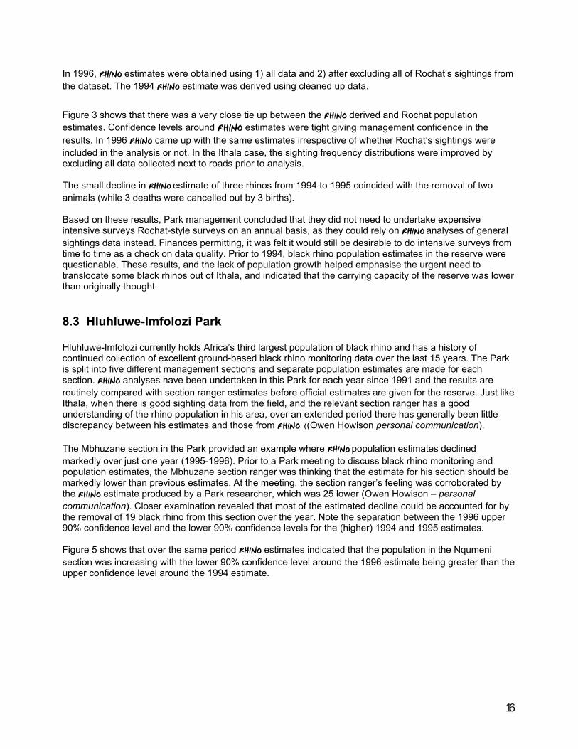
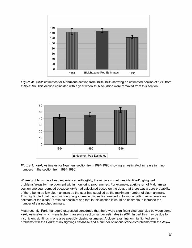
8.3 Hluhluwe-Imfolozi Park Hluhluwe-Imfolozi currently holds Africa’s third largest population of black rhino and has a history of continued collection of excellent ground-based black rhino monitoring data over the last 15 years. The Park is split into five different management sections and separate population estimates are made for each section. RHINO analyses have been undertaken in this Park for each year since 1991 and the results are routinely compared with section ranger estimates before official estimates are given for the reserve. Just like Ithala, when there is good sighting data from the field, and the relevant section ranger has a good understanding of the rhino population in his area, over an extended period there has generally been little discrepancy between his estimates and those from RHINO ((Owen Howison personal communication). The Mbhuzane section in the Park provided an example where RHINO population estimates declined markedly over just one year (1995-1996). Prior to a Park meeting to discuss black rhino monitoring and population estimates, the Mbhuzane section ranger was thinking that the estimate for his section should be markedly lower than previous estimates. At the meeting, the section ranger’s feeling was corroborated by the RHINO estimate produced by a Park researcher, which was 25 lower (Owen Howison – personal communication). Closer examination revealed that most of the estimated decline could be accounted for by the removal of 19 black rhino from this section over the year. Note the separation between the 1996 upper 90% confidence level and the lower 90% confidence levels for the (higher) 1994 and 1995 estimates. Figure 5 shows that over the same period RHINO estimates indicated that the population in the Nqumeni section was increasing with the lower 90% confidence level around the 1996 estimate being greater than the upper confidence level around the 1994 estimate.

17

Figure 4: RHINO estimates for Mbhuzane section from 1994-1996 showing an estimated decline of 17% from 1995-1996. This decline coincided with a year when 19 black rhino were removed from this section. Figure 5: RHINO estimates for Nqumeni section from 1994-1996 showing an estimated increase in rhino numbers in the section from 1994-1996. Where problems have been experienced with RHINO, these have sometimes identified/highlighted problems/areas for improvement within monitoring programmes. For example, a RHINO run of Makhamisa section one year bombed because RHINO had calculated based on the data, that there was a zero probability of there being as few clean animals as the user had supplied as the maximum number of clean animals. This highlighted that the monitoring programme in this section needed to focus on getting as accurate an estimate of the clean/ID ratio as possible; and that in this section it would be desirable to increase the number of ear notched animals. Most recently, Park managers expressed concerned that there were significant discrepancies between some RHINO estimates which were higher than some section ranger estimates in 2004. In part this may be due to insufficient sightings in one area possibly biasing estimates. A closer examination highlighted some problems with the Parks’ rhino sightings database and a number of inconsistencies/problems with the RHINO

0

20

40

60

80

100

120

140

160

1994 1995 1996Mbhuzane Pop Estimates

0

10

20

30

40

50

60

1994 1995 1996

Nqumeni Pop Estimates

18

input dataset which were likely to bias estimates upwards (these issues are currently being addressed). For example the dataset analysed by RHINO was found to have not included a significant number of known deaths and removals, and the resultant RHINO estimates were therefore much higher than they would have been had all the known deaths and removals been taken into account. It will be interesting to see if these discrepancies still exist when RHINO is re-run with a cleaned up dataset. Population estimates using RHINO will of course vary from year to year due to sampling chance, but experience in Hluhluwe-Imfolozi over the years has indicated that the black rhino estimates produced by RHINO are much more precise (and hence less variable) compared to population estimates of other species such as white rhinos obtained from distance sampling along walked line transects (Paul Fatti – personal communication).

8.4 Mkhuze Game Reserve In the past, distance sampling along cut line transects was used to estimate animal numbers in this reserve with the exception of black rhino (estimated using RHINO analysis of sighting re-sighting data). Distance sampling based estimates of white rhino numbers in Mkhuze however were found to yo-yo dramatically from one survey to the next, with estimates sometimes double that of the previous year! When dealing with such valuable animals it made sense to get a better handle on their numbers; and so the Reserve decided to also estimate white rhino numbers using RHINO. The result of this change in technique was that reserve estimates of white rhino became very much more precise and more consistent from year to year.

8.5 Ol Pejeta and Ol Jogi These two Kenyan black rhino popuations are amongst the most intensively monitored black rhino populations anywhere, with the result that both populations are completely known. As part of some recent RHINO training in Kenya, very limited subsets of sightings data from these two parks were analysed by RHINO, and in both cases the RHINO derived population estimates were within 1 or 2 rhino of the actual number of rhinos in these populations.

8.6 Final comments Where there has been good ground coverage over an area, and sufficient sightings have been collected (ideally at least 2 per non trap-happy rhino), RHINO has proved to be reasonably robust, and the results appear reasonable when compared with either the known number of rhinos or expert estimates of numbers by expert rangers in charge of monitoring programmes in their areas. Confidence levels around RHINO derived estimates are usually lower than other population estimation methods (such as distance sampling or intensive block counting). However the fact remains if significant parts of a Park are not sampled, no technique will be able to estimate the number of rhinos in the unsampled areas. In practice, the biggest difficulty has probably been the identification of trap-happy animals when the fit between observed and theoretical truncated Poisson frequency distribututions has not been good making it difficult to reliably define trap-happy animals, and possibly also making some animals in the low sampled are trap-shy animals. In some cases the resultant population estimates have varied depending on the particular trap-happy threshold cut off selected. However, in such cases the poor fit between the observed and theoretical sighting frequency distributions has probably been because one part of a park or section is harder to get to, and as a result is sampled far less frequently than another area. In effect, by pooling all the

19

data together the final sighting frequency distribution is an amalgam of a higher sighting frequency distribution from the more intensively sampled area and a lower sighting frequency distribution from the other less sampled area. This introduces capture (i.e. sighting) heterogeneity violating the assumption that there is an approximately equal chance of each rhino being seen. The solution here is to use a multi-area analysis to produce separate estimates for the two areas which were sampled at different intensities, and combine these sub-estimates, rather than trying to pool all the data together and doing a single analysis. Users could plot sightings of rhinos seen at different frequencies using different symbols, and use this map to define sub-sections for analysis. In some reserves dropping sightings from roads has also helped improve the shape of the observed sighting frequency distributions. There are different stages in monitoring rhino populations; and the desirability of using RHINO varies depending upon which stage you are at with monitoring.

• Initially with little data, RHINO estimates will be imprecise and significantly biased upwards. Little confidence can be placed in the results and confidence levels will also be huge. In such cases it is best to simply use the known minimum until more data have been collected. RHINO will warn users if this is the case.

• Eventually one will collect enough sightings data to use RHINO, and the estimates produced are likely to more accurately reflect the true population size than just the minimum seen. However confidence levels may still be wide.

• As more data are collected RHINO estimate accuracy and precision will improve and the predicted number of identifiable rhino not yet seen will drop.

• Eventually with very high levels of sampling such as at Ol Pejeta or Ol Jogi, you will reach the stage where you know or have seen all the animals in the population, and using RHINO would simply confirm that you can be very confident that you have seen all the animals. When you know all the animals, population estimation techniques such as RHINO are not needed.

RHINO is ideally suited to intermediate sighting frequency situations where the average sighting frequency per non trap-happy rhino ranges from about 2 to 5. In practice in some areas it may be necessary to analyse data collected over a two year period to ensure that average sighting levels are above the recommended minimum of 2 sightings per non trap-happy animal .

20

METHODS

1. Breakdown of a population into segments RHINO breaks down a population into different segments, and estimates the size of each population segment in turn, before combining these estimates together to produce an overall population estimate.

• RHINO distinguishes between independents, defined as F class adult rhino (7+ years old) and E class sub-adults (3½ to 7 years old) on their own, and dependents which are A-D age class rhino calves (less 3½ years old) which are still with their mothers. These calves are not statistically independent of their mothers, and their sightings are therefore not used in the mark-recapture calculations. RHINO estimates the number of calves separately.

• RHINO also distinguishes between independents that have obvious identifying features which can be

recorded by all reliable observers using ear tears and ear notches (identifiable or ID animals) and those which have no or more subtle/harder to record distinguishing features which will not be recorded by all observers all the time (clean animals). For mark-recapture purposes animals treated as clean invariably have ears without any identifying tears or notches.

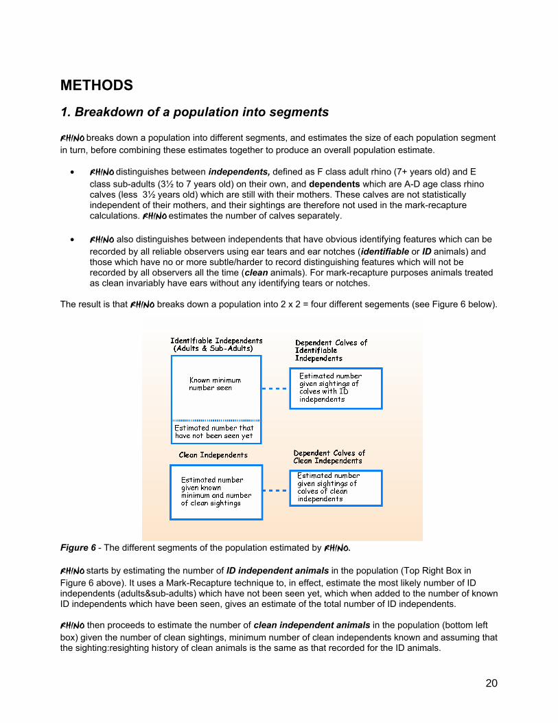
The result is that RHINO breaks down a population into 2 x 2 = four different segements (see Figure 6 below). Figure 6 - The different segments of the population estimated by RHINO. RHINO starts by estimating the number of ID independent animals in the population (Top Right Box in Figure 6 above). It uses a Mark-Recapture technique to, in effect, estimate the most likely number of ID independents (adults&sub-adults) which have not been seen yet, which when added to the number of known ID independents which have been seen, gives an estimate of the total number of ID independents. RHINO then proceeds to estimate the number of clean independent animals in the population (bottom left box) given the number of clean sightings, minimum number of clean independents known and assuming that the sighting:resighting history of clean animals is the same as that recorded for the ID animals.

21

RHINO then proceeds to estimate the number of calves (dependents) of ID independents (Top right box in Figure 6) and then the number of calves of clean independents (Bottom right box in Figure 6). Bootstrapping algorithms are used to estimate calf numbers. These segments are then combined to give total independent and total dependent estimates. These are finally then combined to give the total population estimate. RHINO produces posterior probability distributions for each of the four population segments and the three combined graphs; with the Y axis of these graphs giving the probability the population/segment is each of a range of possible sizes (X axis). Population estimates (mean, median and mode) and the Bayesian equivalent of confidence levels (called credible posterior intervals or CPI) are then derived from these distributions. More complicated forms of analysis are also possible for parks with a number of different sections and where some animals move from section to section. RHINO is also designed to deal with a number of violations of classical Mark-Recapture assumptions such as introductions, deaths, removals, ear-notching of clean animals which makes them identifiable, “sighting-happy” rhinos which are seen very regularly, and the change in status of calves as they grow up to be independent of their mothers (increasing the number of independents and decreasing the number of dependents).

2. Population Estimation of Identifiable (ID) Independents

2.1 The basic "Underhill" Bayesian mark-recapture algorithm used by RHINO RHINO was developed by modifying the basic "Underhill" Bayesian mark-recapture method which estimates the number of individually recognizable animals seen once at a time (Underhill and Fraser 1989). It is the Bayesian analogue of the method due to Craig (1956), which is also known as the de Feu estimate (du Feu et al. 1983). RHINO has adapted the basic “Underhill”method to deal with a number of potential violations of assumptions by real world data. To analyse data collected on multiple discrete surveys one should not use RHINO. In such cases one should rather use the Zucchini-Channing (1986) method which is the appropriate Bayesian analogue of the basic Schnabel mark recapture method. This method was independently developed by Gazey and Staley (1986) and has been termed the GSZC method (Underhill 1989), The Underhill method can be thought of as a special case of the Zucchini—Channing method when survey sample sizes are of size one (Underhill 1989). The “Underhill” method is a basic mark-recapture method which has a number of classical assumptions which are invariably violated by real world black rhino sighting data.

• The basic "Underhill" method deems all animals to be identifiable which works when birds are caught and ringed in a mist-net (the application for which the “Underhill” method was developed). This does not hold for many rhino populations, were some (clean) animals do not have obvious identifying features. Thus the basic “Underhill” method only deals with the independent identifiable (ID) segment of the population. RHINO was specifically developed to also be able to estimate the number of clean rhino.

• The “Underhill” method also assumes the population is closed – that is doesn’t change during the sampling period. To collect enough rhino sightings data it may take as long as two years and during this period rhinos may die, be born, be introduced or removed and clean animals may be ear-

22

notched and made identifiable. Thus rhino populations are likely to be changing in size during the the data collection period and RHINO adapts the basic “Underhill” method to allow for this.

• The “Underhill” method assumes that each individual has an equal chance of being caught. In rhino populations it may be easier to see rhinos in some areas of a park than another, and some “trap-happy” rhinos may be seen much more often than other rhinos if they live in more open areas near frequently traveled routes and nearby staff accommodation. This violates the classical assumption of equal catchability, and again RHINO seeks to adapt the basic “Underhill” method to allow for these violations of this classical assumption.

• The “Underhill” method assumes that the probability of sighting each animal is independent of other animals. This is not the case with rhino where calves are not statistically independent of their mothers. RHINO therefore excludes calf sightings from the mark recapture analyses and uses a bootstrapping approach to separately estimate the number of rhino calves in a population. RHINO has also been modified to handle calves growing up and becoming independent of their mothers.

Before proceeding to see how RHINO deals with these violations of classical assumptions let us first examine the basic “Underhill” method which RHINO has built upon. The basic "Underhill" method starts with the user supplying prior probabilities of the population size being each of a range of values of N from the user specified possible minimum population size (Nmin) up to the user specified maximum population size of the population (Nmax). In most cases, users will specifiy priors which are uninformative with the probability of each possible value of Nj from Nmin to Nmax being set as equal. However if the user does have knowledge about the population, informative priors can be set (where the probabilities of each value of Nj can vary). The probabilities of the population being each of a range of possible values of Nj are updated after each observation. The equation used depends upon whether the sighting is of an animal seen for the first time or a re-sighting during the sampling period. If the ith animal is a first sighting, then the posterior probabilities for each possible value of Nj from Nmin to Nmax are updated using equation (1):

Equation 1. )(Pr)(Pr 1 jij

jji N

NmN

kN −×−

=

After the posterior probabilities have been adjusted the value of m is increased by 1. If the ith animal is a re-sighting then posterior probabilities for each of the j possible value of Nj after sighting i are updated using equation (2):

Equation 2. )(Pr)(Pr 1 jij

ji NNmkN −×=

The value of m remains unchanged In both equations 1 and 2 above: Pri(Nj) = the probability after the ith rhino sighting for each of all the j possible values of population size N

23

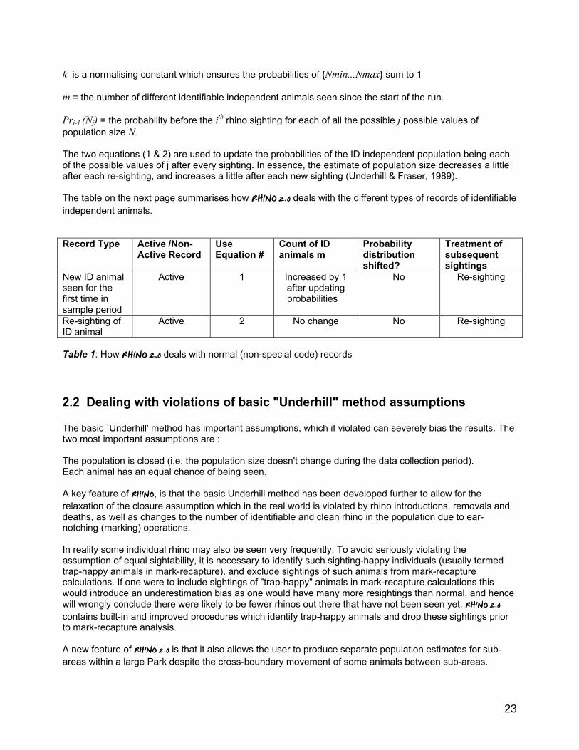
k is a normalising constant which ensures the probabilities of {Nmin...Nmax} sum to 1 m = the number of different identifiable independent animals seen since the start of the run. Pri-1 (Nj) = the probability before the ith rhino sighting for each of all the possible j possible values of population size N. The two equations (1 & 2) are used to update the probabilities of the ID independent population being each of the possible values of j after every sighting. In essence, the estimate of population size decreases a little after each re-sighting, and increases a little after each new sighting (Underhill & Fraser, 1989). The table on the next page summarises how RHINO 2.0 deals with the different types of records of identifiable independent animals. Record Type Active /Non-

Active Record Use Equation #

Count of ID animals m

Probability distribution shifted?

Treatment of subsequent sightings

New ID animal seen for the first time in sample period

Active

1 Increased by 1 after updating probabilities�

No Re-sighting

Re-sighting of ID animal

Active

2 No change No Re-sighting

Table 1: How RHINO 2.0 deals with normal (non-special code) records

2.2 Dealing with violations of basic "Underhill" method assumptions The basic `Underhill' method has important assumptions, which if violated can severely bias the results. The two most important assumptions are : The population is closed (i.e. the population size doesn't change during the data collection period). Each animal has an equal chance of being seen. A key feature of RHINO, is that the basic Underhill method has been developed further to allow for the relaxation of the closure assumption which in the real world is violated by rhino introductions, removals and deaths, as well as changes to the number of identifiable and clean rhino in the population due to ear-notching (marking) operations. In reality some individual rhino may also be seen very frequently. To avoid seriously violating the assumption of equal sightability, it is necessary to identify such sighting-happy individuals (usually termed trap-happy animals in mark-recapture), and exclude sightings of such animals from mark-recapture calculations. If one were to include sightings of "trap-happy" animals in mark-recapture calculations this would introduce an underestimation bias as one would have many more resightings than normal, and hence will wrongly conclude there were likely to be fewer rhinos out there that have not been seen yet. RHINO 2.0 contains built-in and improved procedures which identify trap-happy animals and drop these sightings prior to mark-recapture analysis. A new feature of RHINO 2.0 is that it also allows the user to produce separate population estimates for sub-areas within a large Park despite the cross-boundary movement of some animals between sub-areas.

24

2.3 Independent Identifiable Priors RHINO is a Bayesian technique. To start off an analysis users provide prior probabilities for the independent identifiable population being different values of Nj over a specified range. These prior probabilities are then iteratively updated after each sighting/re-sighting and calculations also take into account additional evidence (such as deaths or removals) to eventually produce the final posterior probability distribution from whci population estimates and the Bayesian equivalent of confidence levels are derived. Priors specify the possible range for Nj as well as provide initial starting probabilities for each value of Nj from Nmin to Nmax. In most case uninformative priors will be selected where the probabilities for each possible value of Nj within the specified range are set equal. It is important to remember that the priors you are initially asked to supply concern only the identifiable independent non-trap-happy segment of the population (and not the whole population). These priors also only refer to numbers likely to be present at the start, and not the end of the analysis period. If animals are added or lost to the population during the sampling period, RHINO automatically adjusts for this. In RHINO 2.0 Users can select to either specify..

• Uninformative ID independent priors (min and max value of Nj with equal probability for each value of Nj in the range)

• Informative ID independent priors (min & max value of Nj and you specify weights for each value of

Nj from Nmin to Nmax).

• Previously saved ID independent priors (users can chose to re-use previously saved priors) 2.3.1 Uninformative Priors With uninformative priors the user only supplies the maximum and minimum possible ID independent population segment size. The probablility of the population being any of the values of N in this range is set as equal. If users have more information about their population they may wish to instead start the analysis with informative priors. Here the user again specifies the bounds within which the true ID independent population size will lie (min and max possible value of N) as well as variable weights for each possible value of N in the specified range. These weights are then used to derive an informative prior probability distribution. When users have limited sightings data and have specific knowledge about a population by setting up informative priors it is impossible to improve estimate precision and accuracy. If you have little a-priori knowledge, it is strongly recommended that you should follow Laplace's principle of insufficient reason and assign equal probabilities to all possible values of N (i.e select Uninformative Priors). RHINO 1.21 offered users the option to maximize the entropy of supplied informative priors with a view to maximizing the influence of the sightings data on the answer. However, in practice whether users decided to maximize the entropy of their informative priors or not made no or almost no difference to the answers produced by RHINO 1.21. For this reason the maximize prior entropy option has been dropped from RHINO 2.O. If this option is selected users in RHINO 2.0 are asked to specify a maximum value of Nj (covering the range of possible population sizes of the identifiable independent segment of the population). RHINO then generates a normalised prior probability distribution (with equal probabilities being assigned for each possible value of Nj in the range Nj = 1 to Nmax). In statistics, normalizing a distribution means to adjust all the probabilities in the distribution so that they sum to 1.

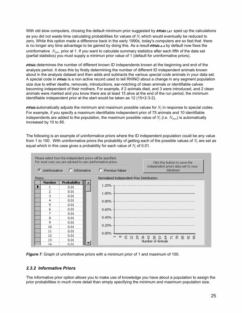
25

With old slow computers, chosing the default minimum prior suggested by RHINO 1,21 sped up the calculations as you did not waste time calculating probabilities for values of Nj which would eventually be reduced to zero. While this option made a difference back in the early 1990s, today's computers are so fast that there is no longer any time advantage to be gained by doing this. As a result RHINO 2.0 by default now fixes the uninformative Nmin prior at 1. If you want to calculate summary statistics after each fifth of the data set (partial statistics) you must supply a minimun prior value of 1 (default for uninformative priors). RHINO determines the number of different known ID independents known at the beginning and end of the analysis period. It does this by firstly determining the number of different ID independent animals known about in the analysis dataset and then adds and subtracts the various special code animals in your data set. A special code in RHINO is a non active record used to tell RHINO about a change in any segment population size due to either deaths, removals, introductions, ear-notching of clean animals or identifiable calves becoming independent of their mothers. For example, if 2 animals died, and 3 were introduced, and 2 clean animals were marked and you know there are at least 15 alive at the end of the run period, the minimum identifiable independent prior at the start would be taken as 12 (15+2-3-2). RHINO automatically adjusts the minimum and maximum possible values for Nj in response to special codes. For example, if you specify a maximum identifiable independent prior of 75 animals and 10 identifiable independents are added to the population, the maximum possible value of Nj (i.e. Nmax) is automatically increased by 10 to 85. The following is an example of uninformative priors where the ID independent population could be any value from 1 to 100. With uninformative priors the probability of getting each of the possible values of Nj are set as equal which in this case gives a probability for each value of Nj of 0.01.

Figure 7: Graph of uninformative priors with a minimum prior of 1 and maximum of 100. 2.3.2 Informative Priors The informative prior option allows you to make use of knowledge you have about a population to assign the prior probabilities in much more detail than simply specifying the minimum and maximum population size.

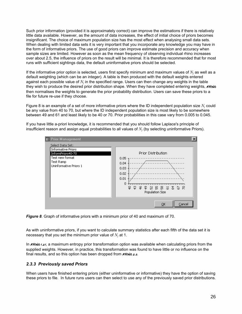
26

Such prior information (provided it is approximately correct) can improve the estimations if there is relatively little data available. However, as the amount of data increases, the effect of initial choice of priors becomes insignificant. The choice of maximum population size has the most effect when analysing small data sets. When dealing with limited data sets it is very important that you incorporate any knowledge you may have in the form of informative priors. The use of good priors can improve estimate precision and accuracy when sample sizes are limited. However as soon as the mean frequency of observing individual rhino increases over about 2.5, the influence of priors on the result will be minimal. It is therefore recommended that for most runs with sufficient sightings data, the default uninformative priors should be selected. If the informative prior option is selected, users first specify minimum and maximum values of Nj as well as a default weighting (which can be an integer). A table is then produced with the default weights entered against each possible value of Nj in the specified range. Users can then change any weights in the table they wish to produce the desired prior distribution shape. When they have completed entering weights, RHINO then normalises the weights to generate the prior probability distribution. Users can save these priors to a file for future re-use if they choose. Figure 8 is an example of a set of more informative priors where the ID independent population size Nj could be any value from 40 to 70, but where the ID independent population size is most likely to be somewhere between 49 and 61 and least likely to be 40 or 70. Prior probabilities in this case vary from 0.005 to 0.045. If you have little a-priori knowledge, it is recommended that you should follow Laplace's principle of insufficient reason and assign equal probabilities to all values of Nj (by selecting uninformative Priors).

Figure 8. Graph of informative priors with a minimum prior of 40 and maximum of 70. As with uninformative priors, if you want to calculate summary statistics after each fifth of the data set it is necessary that you set the minimum prior value of Nj at 1. In RHINO 1.21, a maximum entropy prior transformation option was available when calculating priors from the supplied weights. However, in practice, this transformation was found to have little or no influence on the final results, and so this option has been dropped from RHINO 2.0. 2.3.3 Previously saved Priors When users have finished entering priors (either uninformative or informative) they have the option of saving these priors to file. In future runs users can then select to use any of the previously saved prior distributions.

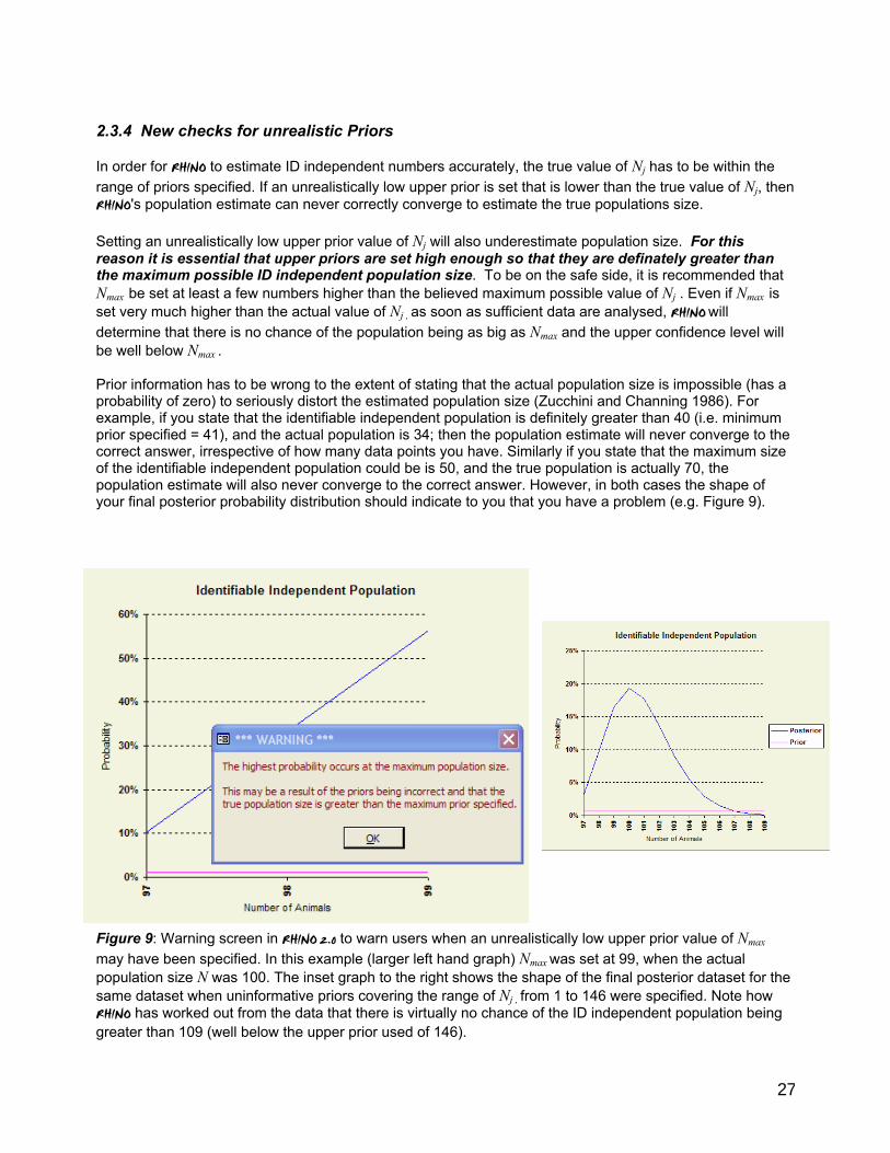
27

2.3.4 New checks for unrealistic Priors In order for RHINO to estimate ID independent numbers accurately, the true value of Nj has to be within the range of priors specified. If an unrealistically low upper prior is set that is lower than the true value of Nj, then RHINO's population estimate can never correctly converge to estimate the true populations size. Setting an unrealistically low upper prior value of Nj will also underestimate population size. For this reason it is essential that upper priors are set high enough so that they are definately greater than the maximum possible ID independent population size. To be on the safe side, it is recommended that Nmax be set at least a few numbers higher than the believed maximum possible value of Nj . Even if Nmax is set very much higher than the actual value of Nj , as soon as sufficient data are analysed, RHINO will determine that there is no chance of the population being as big as Nmax and the upper confidence level will be well below Nmax . Prior information has to be wrong to the extent of stating that the actual population size is impossible (has a probability of zero) to seriously distort the estimated population size (Zucchini and Channing 1986). For example, if you state that the identifiable independent population is definitely greater than 40 (i.e. minimum prior specified = 41), and the actual population is 34; then the population estimate will never converge to the correct answer, irrespective of how many data points you have. Similarly if you state that the maximum size of the identifiable independent population could be is 50, and the true population is actually 70, the population estimate will also never converge to the correct answer. However, in both cases the shape of your final posterior probability distribution should indicate to you that you have a problem (e.g. Figure 9).

Figure 9: Warning screen in RHINO 2.0 to warn users when an unrealistically low upper prior value of Nmax

may have been specified. In this example (larger left hand graph) Nmax was set at 99, when the actual population size N was 100. The inset graph to the right shows the shape of the final posterior dataset for the same dataset when uninformative priors covering the range of Nj , from 1 to 146 were specified. Note how RHINO has worked out from the data that there is virtually no chance of the ID independent population being greater than 109 (well below the upper prior used of 146).

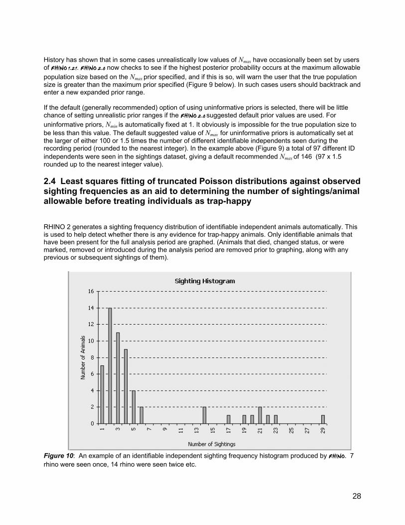
28

History has shown that in some cases unrealistically low values of Nmax have occasionally been set by users of RHINO 1.21. RHINO 2.0 now checks to see if the highest posterior probability occurs at the maximum allowable population size based on the Nmax prior specified, and if this is so, will warn the user that the true population size is greater than the maximum prior specified (Figure 9 below). In such cases users should backtrack and enter a new expanded prior range. If the default (generally recommended) option of using uninformative priors is selected, there will be little chance of setting unrealistic prior ranges if the RHINO 2.0 suggested default prior values are used. For uninformative priors, Nmin is automatically fixed at 1. It obviously is impossible for the true population size to be less than this value. The default suggested value of Nmax for uninformative priors is automatically set at the larger of either 100 or 1.5 times the number of different identifiable independents seen during the recording period (rounded to the nearest integer). In the example above (Figure 9) a total of 97 different ID independents were seen in the sightings dataset, giving a default recommended Nmax of 146 (97 x 1.5 rounded up to the nearest integer value).

2.4 Least squares fitting of truncated Poisson distributions against observed sighting frequencies as an aid to determining the number of sightings/animal allowable before treating individuals as trap-happy RHINO 2 generates a sighting frequency distribution of identifiable independent animals automatically. This is used to help detect whether there is any evidence for trap-happy animals. Only identifiable animals that have been present for the full analysis period are graphed. (Animals that died, changed status, or were marked, removed or introduced during the analysis period are removed prior to graphing, along with any previous or subsequent sightings of them).

Figure 10: An example of an identifiable independent sighting frequency histogram produced by RHINO. 7 rhino were seen once, 14 rhino were seen twice etc.

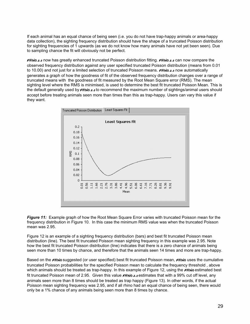
29

If each animal has an equal chance of being seen (i.e. you do not have trap-happy animals or area-happy data collection), the sighting frequency distribution should have the shape of a truncated Poisson distribution for sighting frequencies of 1 upwards (as we do not know how many animals have not yet been seen). Due to sampling chance the fit will obviously not be perfect. RHINO 2.0 now has greatly enhanced truncated Poisson distribution fitting. RHINO 2.0 can now compare the observed frequency distribution against any user specified truncated Poisson distribution (means from 0.01 to 10.00) and not just for a limited selection of truncated Poisson means. RHINO 2.0 now automatically generates a graph of how the goodness of fit of the observed frequency distribution changes over a range of truncated means with the goodness of fit measured by the Root Mean Square error (RMS). The mean sighting level where the RMS is minimised, is used to determine the best fit truncated Poisson Mean. This is the default generally used by RHINO 2.0 to recommend the maximum number of sightings/animal users should accept before treating animals seen more than times than this as trap-happy. Users can vary this value if they want.

Figure 11: Example graph of how the Root Mean Square Error varies with truncated Poisson mean for the frequency distribution in Figure 10. In this case the minimum RMS value was when the truncated Poisson mean was 2.95. Figure 12 is an example of a sighting frequency distribution (bars) and best fit truncated Poisson mean distribution (line). The best fit truncated Poisson mean sighting frequency in this example was 2.95. Note how the best fit truncated Poisson distribution (line) indicates that there is a zero chance of animals being seen more than 10 times by chance, and therefore that the animals seen 14 times and more are trap-happy. Based on the RHINO suggested (or user specified) best fit truncated Poisson mean, RHINO uses the cumulative truncated Poisson probabilities for the specified Poisson mean to calculate the frequency threshold , above which animals should be treated as trap-happy. In this example of Figure 12, using the RHINO estimated best fit truncated Poisson mean of 2.95. Given this value RHINO 2.0 estimates that with a 99% cut off level, any animals seen more than 8 times should be treated as trap happy (Figure 13). In other words, if the actual Poisson mean sighting frequency was 2.95, and if all rhino had an equal chance of being seen, there would only be a 1% chance of any animals being seen more than 8 times by chance.

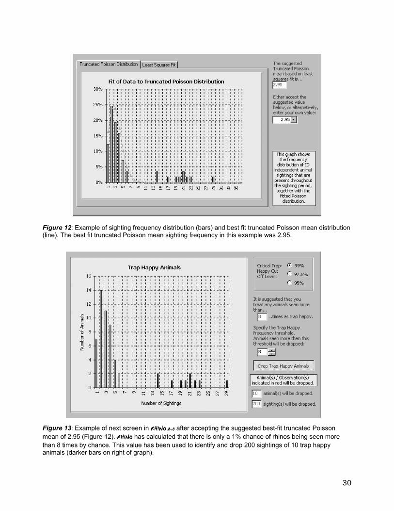
30

Figure 12: Example of sighting frequency distribution (bars) and best fit truncated Poisson mean distribution (line). The best fit truncated Poisson mean sighting frequency in this example was 2.95. Figure 13: Example of next screen in RHINO 2.0 after accepting the suggested best-fit truncated Poisson mean of 2.95 (Figure 12). RHINO has calculated that there is only a 1% chance of rhinos being seen more than 8 times by chance. This value has been used to identify and drop 200 sightings of 10 trap happy animals (darker bars on right of graph).

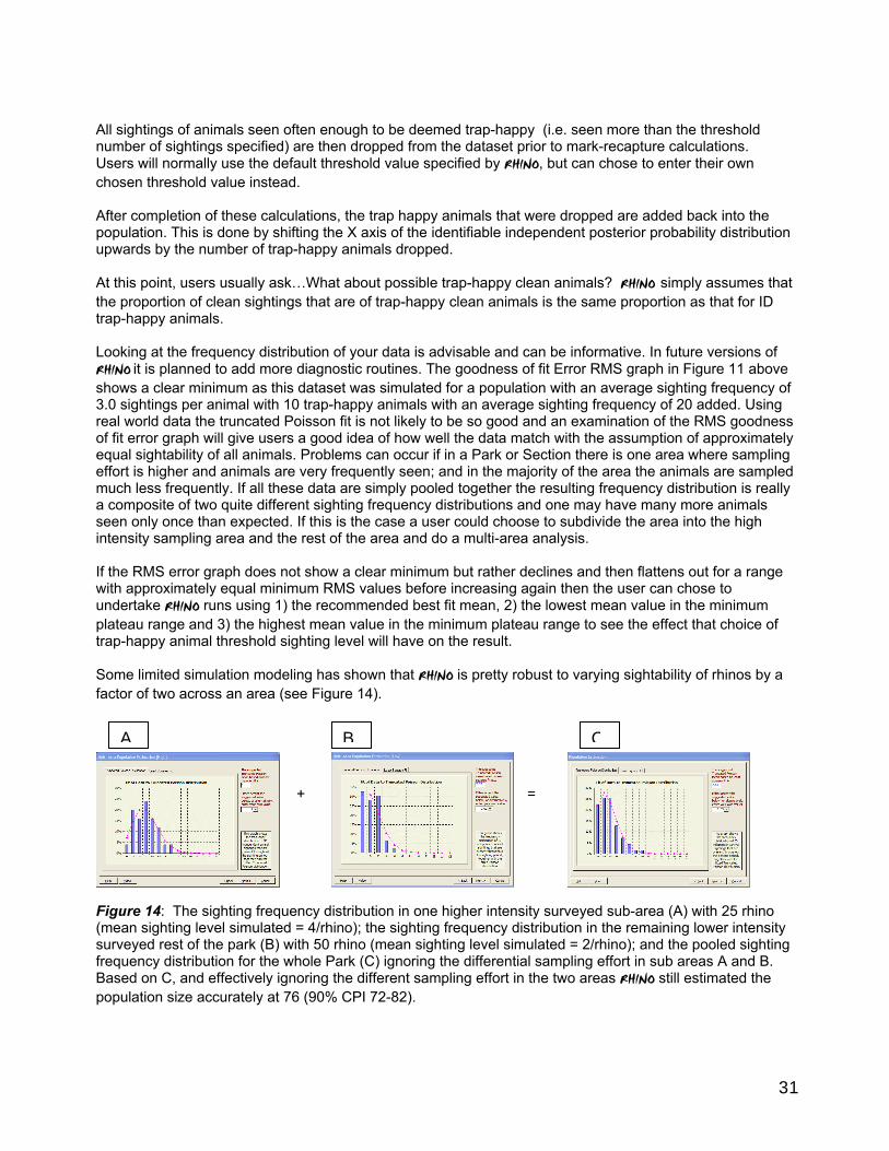
31

All sightings of animals seen often enough to be deemed trap-happy (i.e. seen more than the threshold number of sightings specified) are then dropped from the dataset prior to mark-recapture calculations. Users will normally use the default threshold value specified by RHINO, but can chose to enter their own chosen threshold value instead. After completion of these calculations, the trap happy animals that were dropped are added back into the population. This is done by shifting the X axis of the identifiable independent posterior probability distribution upwards by the number of trap-happy animals dropped. At this point, users usually ask…What about possible trap-happy clean animals? RHINO simply assumes that the proportion of clean sightings that are of trap-happy clean animals is the same proportion as that for ID trap-happy animals. Looking at the frequency distribution of your data is advisable and can be informative. In future versions of RHINO it is planned to add more diagnostic routines. The goodness of fit Error RMS graph in Figure 11 above shows a clear minimum as this dataset was simulated for a population with an average sighting frequency of 3.0 sightings per animal with 10 trap-happy animals with an average sighting frequency of 20 added. Using real world data the truncated Poisson fit is not likely to be so good and an examination of the RMS goodness of fit error graph will give users a good idea of how well the data match with the assumption of approximately equal sightability of all animals. Problems can occur if in a Park or Section there is one area where sampling effort is higher and animals are very frequently seen; and in the majority of the area the animals are sampled much less frequently. If all these data are simply pooled together the resulting frequency distribution is really a composite of two quite different sighting frequency distributions and one may have many more animals seen only once than expected. If this is the case a user could choose to subdivide the area into the high intensity sampling area and the rest of the area and do a multi-area analysis. If the RMS error graph does not show a clear minimum but rather declines and then flattens out for a range with approximately equal minimum RMS values before increasing again then the user can chose to undertake RHINO runs using 1) the recommended best fit mean, 2) the lowest mean value in the minimum plateau range and 3) the highest mean value in the minimum plateau range to see the effect that choice of trap-happy animal threshold sighting level will have on the result. Some limited simulation modeling has shown that RHINO is pretty robust to varying sightability of rhinos by a factor of two across an area (see Figure 14).

+ =

Figure 14: The sighting frequency distribution in one higher intensity surveyed sub-area (A) with 25 rhino (mean sighting level simulated = 4/rhino); the sighting frequency distribution in the remaining lower intensity surveyed rest of the park (B) with 50 rhino (mean sighting level simulated = 2/rhino); and the pooled sighting frequency distribution for the whole Park (C) ignoring the differential sampling effort in sub areas A and B. Based on C, and effectively ignoring the different sampling effort in the two areas RHINO still estimated the population size accurately at 76 (90% CPI 72-82).

A CB

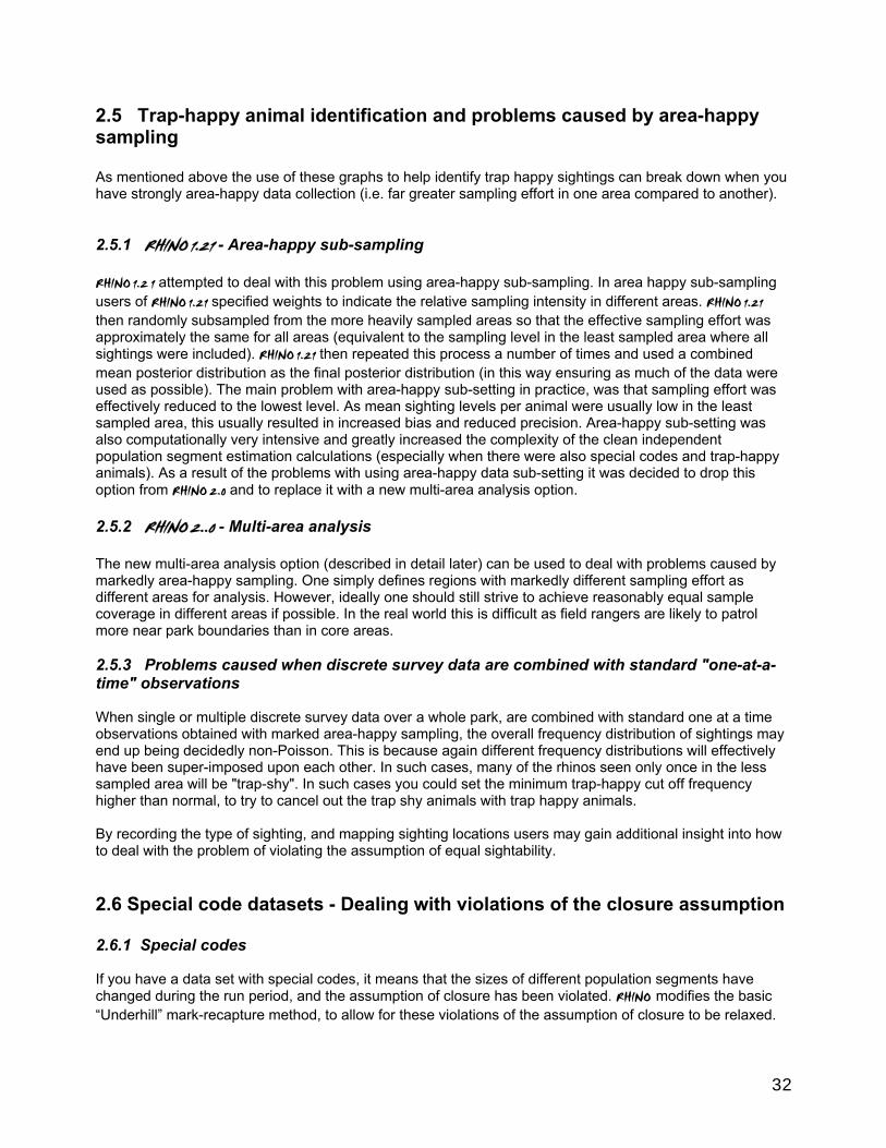
32

2.5 Trap-happy animal identification and problems caused by area-happy sampling As mentioned above the use of these graphs to help identify trap happy sightings can break down when you have strongly area-happy data collection (i.e. far greater sampling effort in one area compared to another). 2.5.1 RHINO 1.21 - Area-happy sub-sampling RHINO 1.2 1 attempted to deal with this problem using area-happy sub-sampling. In area happy sub-sampling users of RHINO 1.21 specified weights to indicate the relative sampling intensity in different areas. RHINO 1.21 then randomly subsampled from the more heavily sampled areas so that the effective sampling effort was approximately the same for all areas (equivalent to the sampling level in the least sampled area where all sightings were included). RHINO 1.21 then repeated this process a number of times and used a combined mean posterior distribution as the final posterior distribution (in this way ensuring as much of the data were used as possible). The main problem with area-happy sub-setting in practice, was that sampling effort was effectively reduced to the lowest level. As mean sighting levels per animal were usually low in the least sampled area, this usually resulted in increased bias and reduced precision. Area-happy sub-setting was also computationally very intensive and greatly increased the complexity of the clean independent population segment estimation calculations (especially when there were also special codes and trap-happy animals). As a result of the problems with using area-happy data sub-setting it was decided to drop this option from RHINO 2.0 and to replace it with a new multi-area analysis option. 2.5.2 RHINO 2..0 - Multi-area analysis The new multi-area analysis option (described in detail later) can be used to deal with problems caused by markedly area-happy sampling. One simply defines regions with markedly different sampling effort as different areas for analysis. However, ideally one should still strive to achieve reasonably equal sample coverage in different areas if possible. In the real world this is difficult as field rangers are likely to patrol more near park boundaries than in core areas. 2.5.3 Problems caused when discrete survey data are combined with standard "one-at-a-time" observations When single or multiple discrete survey data over a whole park, are combined with standard one at a time observations obtained with marked area-happy sampling, the overall frequency distribution of sightings may end up being decidedly non-Poisson. This is because again different frequency distributions will effectively have been super-imposed upon each other. In such cases, many of the rhinos seen only once in the less sampled area will be "trap-shy". In such cases you could set the minimum trap-happy cut off frequency higher than normal, to try to cancel out the trap shy animals with trap happy animals. By recording the type of sighting, and mapping sighting locations users may gain additional insight into how to deal with the problem of violating the assumption of equal sightability.

2.6 Special code datasets - Dealing with violations of the closure assumption 2.6.1 Special codes If you have a data set with special codes, it means that the sizes of different population segments have changed during the run period, and the assumption of closure has been violated. RHINO modifies the basic “Underhill” mark-recapture method, to allow for these violations of the assumption of closure to be relaxed.

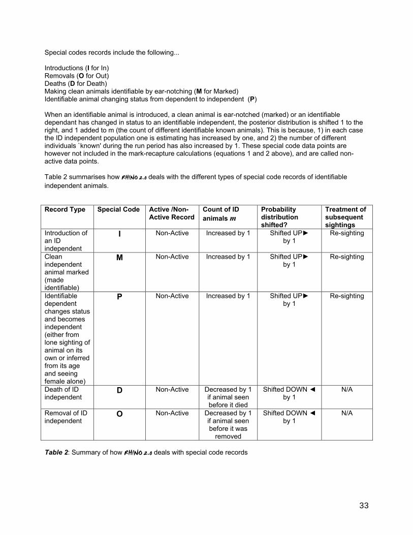
33

Special codes records include the following... Introductions (I for In) Removals (O for Out) Deaths (D for Death) Making clean animals identifiable by ear-notching (M for Marked) Identifiable animal changing status from dependent to independent (P) When an identifiable animal is introduced, a clean animal is ear-notched (marked) or an identifiable dependant has changed in status to an identifiable independent, the posterior distribution is shifted 1 to the right, and 1 added to m (the count of different identifiable known animals). This is because, 1) in each case the ID independent population one is estimating has increased by one, and 2) the number of different individuals `known' during the run period has also increased by 1. These special code data points are however not included in the mark-recapture calculations (equations 1 and 2 above), and are called non-active data points. Table 2 summarises how RHINO 2.0 deals with the different types of special code records of identifiable independent animals. Record Type Special Code Active /Non-

Active Record Count of ID animals m

Probability distribution shifted?

Treatment of subsequent sightings

Introduction of an ID independent

I Non-Active

Increased by 1 �

Shifted UP► by 1

Re-sighting

Clean independent animal marked (made identifiable)

M Non-Active Increased by 1 Shifted UP► by 1

Re-sighting

Identifiable dependent changes status and becomes independent (either from lone sighting of animal on its own or inferred from its age and seeing female alone)

P Non-Active Increased by 1 Shifted UP► by 1

Re-sighting

Death of ID independent

D Non-Active Decreased by 1 if animal seen before it died

Shifted DOWN ◄ by 1

N/A

Removal of ID independent

O Non-Active Decreased by 1 if animal seen before it was

removed

Shifted DOWN ◄ by 1

N/A

Table 2: Summary of how RHINO 2.0 deals with special code records

34

Subsequent sightings of marked or introduced animals are treated as re-sightings in the mark recapture analysis (equation 2 above). This is because the variable m will have been adjusted to include them. Special code observations or ear-notched animals at the time of marking are treated as non-active records in RHINO 2.0, because in contrast to previous versions of RHINO, RHINO 2.0 assumes ear-notching teams will not be recording all animals seen during ear-notching operations (including identifiable animals). Similarly, if an identifiable animal is removed or dies the posterior distribution is shifted down one. If the animal was sighted before it effectively left that population segment, the variable m is also reduced by 1. Finally at the end of mark-recapture calculations the resulting posterior distribution is then shifted up by the number of trap-happy animals dropped prior to the mark-recapture calculations. RHINO therefore automatically adjusts the allowable upper and lower bounds of the posterior distributions. 2.6.2 Dealing with incomplete independent mortality records Ecoadvice staff in Hluhluwe-Imfolozi Park identified a problem that sometimes the ears of some carcasses have been eaten by Hyenas and it is not possible to determine whether an independent animal that died was an ID animal or was clean. Such records are deemed incomplete and before were therefore excluded from RHINO analyses. Ignoring incomplete mortality records where you are not sure if the animal was identifiable or not will act to bias RHINO estimates upwards. While it is hoped to modify a future version of RHINO to be able to handle incomplete independent mortality records, users of RHINO 2.0 can in the interim manually fix this problem in two ways. Option 1: Proceed without special codes for these incomplete mortalities, and at the end of the analysis reduce the total independent population estimate by the number of incomplete independent mortalities. It will also be necessary to reduce the estimate of the number of calves by the same proportion. For example if one reduces the total independent estimate by 2.5%, then the total number of calves and the total population estimate also need to be reduced by 2.5%. Option 2: Another way to handle this problem is to enter special code mortality records for these incomplete mortalities. To do this one first has to allocate the mortalities as either ID or clean. Supposing the estimated proportion of the independent population was 60% and one has 5 incomplete mortality records, one could allocate 3 (60%) as ID mortalities and the remaining 2 as clean mortalities. The next step is to find suitable names for the deemed ID mortalities. Simulations reveal that one should use names of ID animals seen during the analysis period before the mortality event, but which were not seen after. If three mortalities were deemed to be of ID animals, then three different names will be needed. Don’t use names of animals which have been seen previously but have not been seen during the analysis period in question. This analysis approach will automatically make allowances for calves, and there will be no need to change any of the estimates produced by RHINO. You will however need to make a note somewhere which ID mortality records were deemed ID mortalities which were initially incomplete mortality records; in case rhinos with any of the names you supplied are seen later in the future.

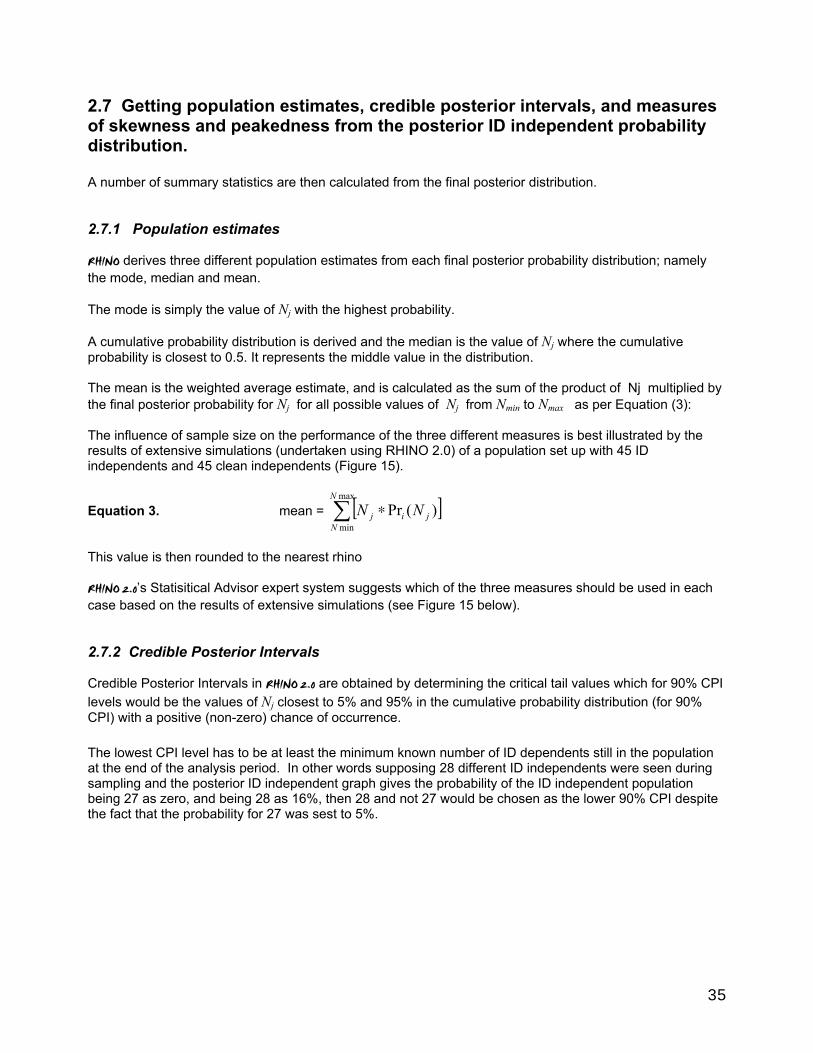
35

2.7 Getting population estimates, credible posterior intervals, and measures of skewness and peakedness from the posterior ID independent probability distribution. A number of summary statistics are then calculated from the final posterior distribution. 2.7.1 Population estimates RHINO derives three different population estimates from each final posterior probability distribution; namely the mode, median and mean. The mode is simply the value of Nj with the highest probability. A cumulative probability distribution is derived and the median is the value of Nj where the cumulative probability is closest to 0.5. It represents the middle value in the distribution. The mean is the weighted average estimate, and is calculated as the sum of the product of Nj multiplied by the final posterior probability for Nj for all possible values of Nj from Nmin to Nmax as per Equation (3): The influence of sample size on the performance of the three different measures is best illustrated by the results of extensive simulations (undertaken using RHINO 2.0) of a population set up with 45 ID independents and 45 clean independents (Figure 15).

Equation 3. mean = [ ]∑ ∗max

min)(Pr

N

Njij NN

This value is then rounded to the nearest rhino RHINO 2.0’s Statisitical Advisor expert system suggests which of the three measures should be used in each case based on the results of extensive simulations (see Figure 15 below). 2.7.2 Credible Posterior Intervals Credible Posterior Intervals in RHINO 2.0 are obtained by determining the critical tail values which for 90% CPI levels would be the values of Nj closest to 5% and 95% in the cumulative probability distribution (for 90% CPI) with a positive (non-zero) chance of occurrence. The lowest CPI level has to be at least the minimum known number of ID dependents still in the population at the end of the analysis period. In other words supposing 28 different ID independents were seen during sampling and the posterior ID independent graph gives the probability of the ID independent population being 27 as zero, and being 28 as 16%, then 28 and not 27 would be chosen as the lower 90% CPI despite the fact that the probability for 27 was sest to 5%.

36

Figure 15: Example of Identifiable Independent population segment posterior distribution showing shaded 90% Credible Posterior Intervals (CPI). The lower 90% CPI value in this case was 97 as this was the closest value of Nj to 5% in a cumulative probability distribution derived from this graph. Similarly 104 was selected as the upper 90% CPI level as it was (just) the closest value of Nj to 95% in the cumulative probability distribution derived from the data in this graph. 2.7.3 Measure of Skewness Skewness is a measure of the asymmetry of the data around the sample mean. If skewness is negative, the data are spread out more to the left of the mean than to the right. If skewness is positive, the data are spread out more to the right. The skewness of the normal distribution (or any perfectly symmetric distribution) is zero. The skewness of each distribution is defined as

Equation 4. skewness = 3

3)(σ

µ−Ε x

where µ is the mean of x,σ is the standard deviation of x, and E(t) represents the expected value of the quantity t When x represents a sample from a population, the skewness of x is biased, that is, it will tend to differ from the population skewness by a systematic amount that depends on the size of the sample. The unbiased skewness of x is calculated as follows:

Equation 5. unbiased skewness = 31

3

)2()1(

)(

σ

µ

−−

−∑=

NN

xNN

ii

37

where N is the number of data points or samples in x. RHINO 2.0 calculates the unbiased skewness of an estimated population distribution. This measure is primarily to provide additional data to assist the developers of RHINO improve the advice given by the inbuilt statistical advisor expert system in future versions of RHINO. 2.7.4 Measure of Peakedness The peakedness of a distribution is simply calculated as Equation 6. peakedness = max Nj of the posterior distribution / (CPIMax – CPIMin + 1) where CPI refers to the 90% Credible Posterior Intervals This measure is also primarily to provide additional data to assist the developers of RHINO improve the advice given by the inbuilt statistical advisor expert system in future versions of RHINO.

2.8 Effect of small sample biases on ID independent estimates If insufficient data are used, ID independent estimates will on average be biased upwards. This is especially the case when very uninformative priors are used. The reason for this is that during the early stages of the analysis the lower end of the posterior distribution is altered faster (as animals are seen) than the upper end of the distribution. The posterior distribution will therefore tend to initially be skewed with a long tail to the right. In such cases, the mean will be bigger than the median which in turn will be bigger than the mode. As sample sizes increase so these three measures of central tendency should converge. The closeness of these three estimates is a good indicator of how good your answer is. Overestimation bias is likely to be very severe whenever there are fewer independent observations than the number of rhino. Limited simulation modelling of a small population indicated that ideally the observation number/rhino should preferably exceed 2. The problem is most serious when very uninformative priors are used were used and the population being estimated is small. Figure 16 illustrates the influence of sample size on the performance of the three different population estimates (mode, median and mode). Note how…

• RHINO on average produces seriously upwardly biased estimates (all 3 measures) when sample sizes are very low (average sighting frequency of 0.33 per rhino). RHINO's built-in Statistical Advisor expert system will warn users when this is likely to have happened. In such cases one should simply use the minimum known and collect more data to enable a better population estimate to be made.

• Although not shown above confidence levels around these estimates are also unacceptably large when sample sizes are small. Overestimation bias is reduced as sample size increases with the mode being the first measure to become unbiased around average sighting frequencies of 1 per rhino.

• As sighting frequencies increase further the mode becomes slightly negatively biased and the median becomes the best estimator.

• It is only at high average sighting frequencies that the mean becomes the most unbiased estimator of ID independent number. At high sampling intensities the three measures converge.

RHINO's built-in Statistical Advisor expert system recommends to users which estimator is likely to produce the best population estimate.

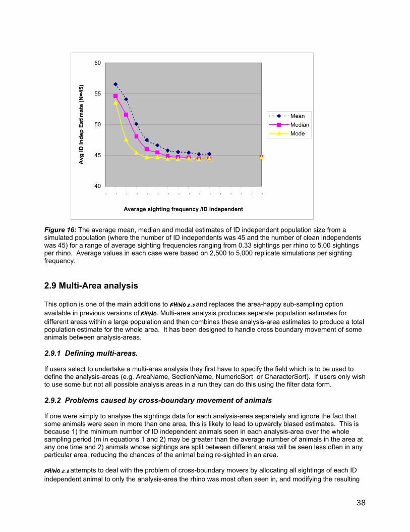
38

Figure 16: The average mean, median and modal estimates of ID independent population size from a simulated population (where the number of ID independents was 45 and the number of clean independents was 45) for a range of average sighting frequencies ranging from 0.33 sightings per rhino to 5.00 sightings per rhino. Average values in each case were based on 2,500 to 5,000 replicate simulations per sighting frequency.

2.9 Multi-Area analysis This option is one of the main additions to RHINO 2.0 and replaces the area-happy sub-sampling option available in previous versions of RHINO. Multi-area analysis produces separate population estimates for different areas within a large population and then combines these analysis-area estimates to produce a total population estimate for the whole area. It has been designed to handle cross boundary movement of some animals between analysis-areas. 2.9.1 Defining multi-areas. If users select to undertake a multi-area analysis they first have to specify the field which is to be used to define the analysis-areas (e.g. AreaName, SectionName, NumericSort or CharacterSort). If users only wish to use some but not all possible analysis areas in a run they can do this using the filter data form. 2.9.2 Problems caused by cross-boundary movement of animals If one were simply to analyse the sightings data for each analysis-area separately and ignore the fact that some animals were seen in more than one area, this is likely to lead to upwardly biased estimates. This is because 1) the minimum number of ID independent animals seen in each analysis-area over the whole sampling period (m in equations 1 and 2) may be greater than the average number of animals in the area at any one time and 2) animals whose sightings are split between different areas will be seen less often in any particular area, reducing the chances of the animal being re-sighted in an area. RHINO 2.0 attempts to deal with the problem of cross-boundary movers by allocating all sightings of each ID independent animal to only the analysis-area the rhino was most often seen in, and modifying the resulting

40

45

50

55

60

. . . . . . . . . . . . . . . .

Average sighting frequency /ID independent

Avg

ID In

dep

Estim

ate

(N=4

5)

MeanMedianMode

39

population estimates using a correction factor. This in effect what Owen Howison was doing to produce separate section estimates for Hluhluwe-Imfolozi Park using RHINO 1.21, although this process wasn’t automated. 2.9.3 Sightings Cross-tabulation RHINO 2.0 starts a multi-area analysis by generating a table listing the total the number of active sightings of each ID independent animal in each analysis-area, as well as the total number of sightings of each ID independent animal (in all analysis-areas). 2.9.4 Allocation of cross boundary sightings for analysis purposes For mark-recapture analysis purposes, RHINO 2.0 then allocates all sightings of each animal to the area they were most frequently seen in. In the case of tied frequencies, random numbers are used to decide which analysis-area to allocate the sightings to. The crosstablulation table documents which analysis-areas sightings of each ID independent animal were allocated to, as well as the % of total sightings of the animal that were made in this area. 2.9.5 Cross-boundary movement correction factor (Xboundary CF) Allocation of some cross-boundary sightings can result in some analysis areas having a greater or smaller number of "sightings" after re-allocation of some cross-boundary sightings compared to before. This can lead to over- or under-estimation biases in the different analysis-areas. While these biases are likely to cancel each other out over the park as a whole, management of a large park invariably will want to undertake a multi-area analysis as accurate and separate population estimates are neded for each area/section in the park. As the latter may be used to decide how many rhinos to move from each area, it is important to try to ensure population estimates for the different analysis areas are as accurate as possible. RHINO 2.0 calculates and uses a cross-boundary correction factor (Xboundary CF) to reduce such biases. The XboundaryCF correction factor is calculated using Equation (7):

Equation 7. XboundaryCF for Areak = k

k

XY

Where… k = Analysis area k Y = Total number of sightings of ID independent animals in analysis-areak prior to re-allocation of cross-boundary sightings X = Total Number of sightings of ID independent animals in analysis-areak after re-allocation of cross-boundary sightings

• Analysis-areas with more sightings after re-allocation of cross-boundary sightings therefore get Xboundary CF's that are < 1.

• Analysis-areas with fewer sightings after re-allocation of cross-boundary sightings have Xboundary

CF's that are >1.

• Analysis-areas with the same number of observations before and after re-allocation get Xboundary CF's of 1.

For example, let us suppose there were 112 ID sightings in analysis-areak before re-allocation of cross-boundary sighting records and 125 sightings in analysis-areak after re-allocation. The Xboundary correction factor for analysis-areak would therefore be 112/125 = 0.8960.

40

In practice the majority of rhino will only be seen in one area. As only a fraction of a rhino population are cross boundary movers, crossboundary correction factors in practice will tend to be close to 1. 2.9.6 Initial Analysis-Area population estimation Analysis then proceeds for each analysis-area separately, with ID independent and clean independent posterior distributions calculated as per normal using the new datasets created for each area following reallocation of cross boundary ID independent sightings. Trap-Happy animals are dealt with and dropped in the same manner as before. 2.9.7 Using the XboundaryCF to bias-correct mean population estimates The unrounded mean ID independent estimate, calculated for analysis-areak using equation 3 is then multiplied by the XboundaryCF's for that specific analysis-area. This is then rounded to the nearest integer to produce a bias corrected mean population estimate for that analysis-area. For example, supposing the uncorrected unrounded mean estimate for analysis-areak was 42.1034 and the Xboundary correction factor for this analysis-area was 0.8960. The XboundaryCF corrected mean estimate for this analysis-area would be 38 (37.7246 rounded up). 2.9.8 Calculation of bias-corrected mode and median population estimates and bias corrected CPI's RHINO 2.0 then subtracts the unrounded uncorrected mean estimate from the unrounded bias-corrected mean estimate. The answer is then rounded to the nearest integer and the resultant posterior ID probability distribution is shifted up (if +ve) or down (if -ve) by this amount to produce a revised ID independent posterior distribution. Bias corrected estimates of the mode, median and CPI levels are then obtained from this shifted posterior distribution as before. In our hypothetical example above the ID independent posterior distribution for analysis-areak would be shifted down by 4 (37.7246 - 42.1034 = - 4.3788 rounded to -4). If using the uncorrected posterior distribution the mode, median and CPI levels were 40, 41 and 39-48 the corrected values would be 36, 37 and 25-43 respectively. 2.9.9 Uncorrected estimates These are also documented in the RHINO 2.0 output report. While it is recommended that users always use Xboundary bias corrected population estimates and CPI's for individual analysis-areas, the uncorrected analysis-areas are also given in the output report. 2.9.10 Calculation of total Park ID Independent Population Estimates and CPI's Analysis proceeds for each analysis-area one at a time. The final ID independent posterior probability distributions for each analysis area are simply combined to produce a total ID independent distribution from which total park ID independent population estimates can be derived. The procedure for adding two distributions together is straight forward and is done as follows: Let the distributions to be added = Y and Z; with population sizes {Ymin, Ymin+1,...Yi,...Ymax} and {Zmin, Zmin+1,...Zj,...Zmax} with probabilities of occurrence = Pr(Yi) and Pr(Zi) respectively.

41

and let the joined distribution = G; with possible population sizes {Gmin,...Gij,...Gmax};, and Pr(Gij) respectively. Then for every combination of Yi and Zj , values of both Gij and Pr(Gij) are derived from equation's 8 and 9 below: Equation 8. )Pr()Pr()Pr( jiij ZYG ∗= Equation 9. ∑

=

=TiGij

iji GT )Pr()Pr(

The values of Pr(Gij) for each of the possible values of Gij are then summed (and if necessary normalized) to give the joined probability distribution. Summary statistics are then calculated from this distribution as before. In a multi-area analysis, after estimating the ID independents posterior distribution for an area, analysis would proceed just the same as a straight analysis to calculate posterior distributions for clean independents, then dependents and finally total numbers. The process is then repeated for each analysis area in turn. Finally once data from all analysis areas have been analysed the various posterior distributions for each area are combined to produce park level estimates for each population segement as well as totals.

3. POPULATION ESTIMATION OF CLEAN INDEPENDENTS

3.1 Assumptions The two main assumptions behind the estimation of clean animal population size are that: 1. Clean animals are likely to have similar mark-recapture histories to identifiable animals. If most of your sightings of ID animals were new sightings rather than resightings, it seems reasonable to assume that most of the clean sightings were probably also of animals being seen for the first time. Conversely, if almost all the sightings of ID animals at the end of a run are resightings, the same is likely to be true for clean sightings. 2. The degree of trap-happiness of clean animals is the same as that for ID animals.

3.2 Basic approach for estimating the number of clean independents RHINO generates a clean independent population probability distribution by combining:

• a weighting probability function derived from results of mark-recapture analysis of identifiable animals

with

• the estimated binomial distribution of clean animal observation number. Before considering more complicated analysis, let us first consider how RHINO estimates the clean population in the simplest of cases (no area-happy or trap-happy observations and no special codes)

42

3.2.1 Stage 1 : Derivation of the Weighting Function When there are no special code animals, RHINO does the main mark-recapture analysis of ID independent animals first in the standard manner described above. The relationship between mark-recapture history and observation number is given by the final posterior distribution of identifiable independent population size. The total number of active observations of ID independents in the dataset used to produce the ID independent posterior distribution (including the trap-happy ID independent observations that were dropped from mark-recapture calculations) is called the weight denominator (D) by RHINO. RHINO simply divides each of the estimated identifiable independent population sizes on the X axis of the final mark-recapture ID independent posterior distribution by the weight denominator, D, to change the posterior ID independent probability distribution to a distribution of weighting factors and their probabilities. The probabilities remain the same – all that changes is that the various values of ID independent number are replaced with a series of weighting factors. The weighting factors simply measure the relationship between total ID independent population size (both normal and trap-happy animals) and sample size (all ID independent active observations irrespective of whether they were of trap-happy animals or not). It is important to understand that the derived weighting factors take into account all ID independent animals in the population and their sightings, irrespective of whether or not some of them are trap happy. This is important, given the assumption that the degree of trap-happiness of clean animals is the same as that for ID animals. Supposing that our ID independent data set contains 100 observations (D=100), for an ID population size of 50. For the actual ID independent population size of 50 the weighting factor would be 0.5 (i.e. 50/100). However, as we are dealing with an estimated posterior distribution this will include a range of possible values of Nj and not just the actual value of N. Supposing that the values of Nj in the final posterior distribution covered the range of 45 up to 59 we can similarly convert each of these Nj values to weighting factors Wi by dividing them by D. The Wi for 45 would be 0.45 etc.. The mark-recapture posterior distribution together with sample size therefore gives us the probabilities of getting each different weighting factor. All we have done is to replace the estimates of ID independent number Nj along the X axis of the final posterior distribution with a series of weighting factors, Wi (obtained by simply by dividing the vaues of Nj by D). By multiplying a weighting factor (e.g. 0.50) by the total number of ID observations (100) we return the original estimate of ID population size, Nj (in this case 50). If we extend this logic a little... We also know the number of clean observations in our sample (suppose this is 40), and by multiplying each of the derived weighting factors Wi by this number we can transform the weights into estimates of clean animal number. Given a total of 40 clean sightings, the estimated clean population size for a Wi of 0.50 would be 20 (i.e. 0.5 * 40) . We can proceed to estimate the number of clean independents estimated for each value of Wi in the graph. The clean estimate for a Wi of 0.45 would for example be 18. Supposing instead that 10 of the 50 ID independents were trap happy. Let us assume that there were 100 observations of 40 non trap-happy animals, and another 100 observations of the 10 trap-happy animals this gives us an overall average sighting frequency of 4 per rhino (double the earlier example). Our weighting factor Wi when Nj = N = 50 in this case would be 0.25 (50/200). Supposing we still only had 40 clean independent sightings this Wi would estimate the clean populations size at 10. In this case allowances have been made for the assumption that a similar proportion of clean animals were trap-happy. However we know that the total number of clean observations (40 in both examples above) will be subject to binomial sampling error. RHINO therefore repeats the procedure, obtaining probability functions for each

43

possible value of total clean observation number. But, before we can do this, we need to estimate the probability of getting different clean observation numbers in our sample.

3.2.2. Stage 2 : Estimation of the distribution of Clean Observation Number The distribution of Clean observation number is estimated using the binomial distribution given 1) the proportion of observations which are clean, and 2) the total number of observations. RHINO takes these parameters and uses equation 10 below, to estimate the binomial probability of obtaining different numbers of clean observations in your data set. RHINO starts with the observed number of clean observations and works upwards by one observation at a time, until the estimated probability of occurrence is less than 0.00001. It then repeats the procedure downwards; again until probabilities become very small. Only Clean observation numbers with probabilities $ 0.00001 are included in the distribution of possible clean observation number. The cumulative probabilities in the distribution are finally normalised so that they sum to 1. The probabilities of obtaining each possible clean observation number Pr(Oj) out of a random sample size of N (total number of independent observations) are calculated using equation 10.

Equation 10. OjNOj

jjj qp

ONONO −

−=

)!(!!)Pr(

where… N = Total number of observations of independent animals; Oj = Possible clean observation number; p = Proportion of independent observations that are clean for a given Oj (number from 0 to 1) q = Proportion of independent observations that are not clean for a given Oj (number from 0 to 1). ! stands for factorial (for example 2! = 1*2 = 2; 4! = 1*2*3*4 = 24 ; N.B. 0! = 1) To avoid problems of numeric overflow, RHINO uses logarithms of factorials in its calculations, and then takes the anti-log of the result.

3.2.3 Stage 3 : Estimation of the Clean population probability distribution The clean population distribution is generated by combining the binomial distribution of clean animal observation number (Stage 2) with the weighting probability function derived from the final ID independent posterior probability distribution (Stage 1). Let… Weights = Wi for values over the range {Wmin, Wi,..., Wmax}, with a probability of occurrence = Pr(Wi), Clean observation number = O for values over the range {Omin, Omin+1,...Oj,...Omax} with a probability of occurrence = Pr (Oj)

44

For all possible combinations of Wi and Oj the possible Clean population sizes Cij and their probabilities Pr(Cij) are calculated by formulas 11 and 12. Equation 11. )Pr( jiij OWC ∗= Equation 12. )Pr()Pr()Pr( jiij OWC ∗= The clean population estimates (Cij) are then rounded to the nearest integer. The probabilities for each possible clean population size are then summed (and if necessary normalised) to produce the population distribution for clean independants.

3.2.4 Stage 4 : Incorporation of prior knowledge to refine final distribution If it is known that you have at least x clean animals, then this knowledge can be incorporated into the clean population size distribution by setting all probabilities for clean number Cij < x to 0. All upper values of Cij with probabilities of occurrence < 0.000001 are also dropped from the distribution. The resulting distribution is then normalised so that the cumulative probabilities sum to 1. The total number of different rhino identified by key observers only (on more subtle/harder to record features) can be used to provide RHINO with an estimate of the minimum number of clean independents. In RHINO 2.0 users can no longer bias clean independent estimates downwards by specifying unrealistically low upper clean priors. Users can however supply an estimated maximum clean number and RHINO will calculate and graph the probability, based on the data collected, that the actual clean number is higher than the specified value. If this probability is significant then the two possible most likely explanations are ..

• The evidence is indicating that the clean population segment is much bigger than you thought it was; or

• Incomplete sightings have somehow incorrectly also got classified as clean sightings and included in your dataset, leading to an overestimate of clean independent number.

3.2.5 Stage 5 : Calculation of summary statistics The mode, median, mean and specified credible posterior intervals are then calculated as before from the final clean independent distribution. The statistical advisor advises the user on which measure is likely to be the best estimate. For the first time RHINO 2.0 offers advice specific to the estimation of clean independent number. Simulation modelling has revealed that depending upon the level of sampling, either the mode or median (but not the mean) will be the best estimate of clean independent number. Figure 17 below shows that like the ID independent estimator, RHINO’s clean independent estimator is seriously biased upwards when sample sizes are low. As sampling effort increases the mode is the first estimator to become unbiased followed by the median. However at sampling intensities of 3.33 the mean still is slightly positively biased. Figure 17 shows that it is only at very high sampling intensities (mean of 5 sightings per animal) that all three estimates converge.

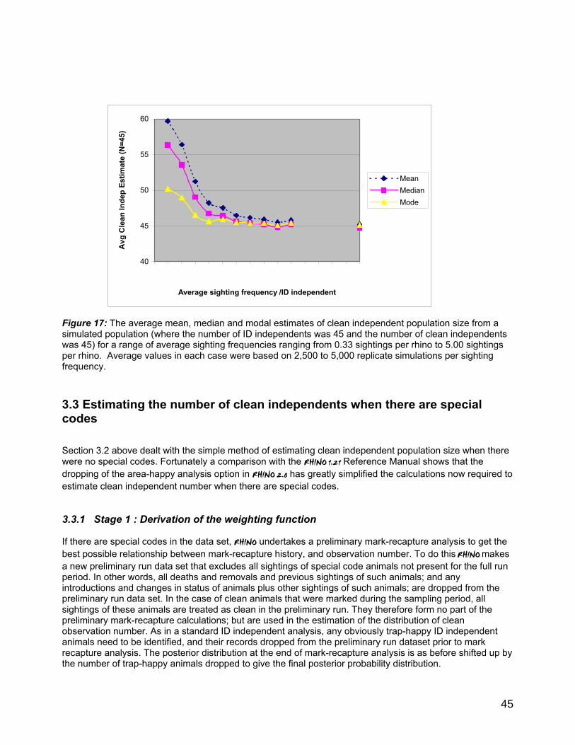
45

Figure 17: The average mean, median and modal estimates of clean independent population size from a simulated population (where the number of ID independents was 45 and the number of clean independents was 45) for a range of average sighting frequencies ranging from 0.33 sightings per rhino to 5.00 sightings per rhino. Average values in each case were based on 2,500 to 5,000 replicate simulations per sighting frequency.

3.3 Estimating the number of clean independents when there are special codes Section 3.2 above dealt with the simple method of estimating clean independent population size when there were no special codes. Fortunately a comparison with the RHINO 1.21 Reference Manual shows that the dropping of the area-happy analysis option in RHINO 2.0 has greatly simplified the calculations now required to estimate clean independent number when there are special codes. 3.3.1 Stage 1 : Derivation of the weighting function If there are special codes in the data set, RHINO undertakes a preliminary mark-recapture analysis to get the best possible relationship between mark-recapture history, and observation number. To do this RHINO makes a new preliminary run data set that excludes all sightings of special code animals not present for the full run period. In other words, all deaths and removals and previous sightings of such animals; and any introductions and changes in status of animals plus other sightings of such animals; are dropped from the preliminary run data set. In the case of clean animals that were marked during the sampling period, all sightings of these animals are treated as clean in the preliminary run. They therefore form no part of the preliminary mark-recapture calculations; but are used in the estimation of the distribution of clean observation number. As in a standard ID independent analysis, any obviously trap-happy ID independent animals need to be identified, and their records dropped from the preliminary run dataset prior to mark recapture analysis. The posterior distribution at the end of mark-recapture analysis is as before shifted up by the number of trap-happy animals dropped to give the final posterior probability distribution.

40

45

50

55

60

Average sighting frequency /ID independent

Avg

Cle

an In

dep

Estim

ate

(N=4

5)

MeanMedianMode

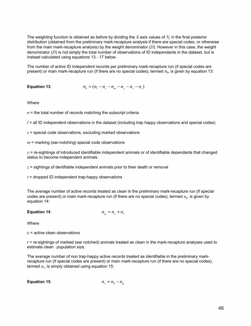
46

The weighting function is obtained as before by dividing the X-axis values of Nj in the final posterior distribution (obtained from the preliminary mark-recapture analysis if there are special codes, or otherwise from the main mark-recapture analysis) by the weight denominator (D). However in this case, the weight denominator (D) is not simply the total number of observations of ID independants in the dataset, but is instead calculated using equations 13 - 17 below. The number of active ID independent records per preliminary mark-recapture run (if special codes are present) or main mark-recapture run (if there are no special codes), termed nb, is given by equation 13: Equation 13. )( tzymslb nnnnnnn −−−−−= Where n = the total number of records matching the subscript criteria l = all ID independent observations in the dataset (including trap happy observations and special codes) s = special code observations, excluding marked observations m = marking (ear-notching) special code observations y = re-sightings of introduced identifiable independent animals or of identifiable dependants that changed status to become independent animals. z = sightings of dentifiable independent animals prior to their death or removal t = dropped ID independent trap-happy observations The average number of active records treated as clean in the preliminary mark-recapture run (if special codes are present) or main mark-recapture run (if there are no special codes), termed ng, is given by equation 14: Equation 14. rcg nnn += Where c = active clean observations r = re-sightings of marked (ear notched) animals treated as clean in the mark-recapture analyses used to estimate clean population size. The average number of non trap-happy active records treated as identifiable in the preliminary mark-recapture run (if special codes are present) or main mark-recapture run (if there are no special codes), termed nv, is simply obtained using equation 15: Equation 15. gbv nnn −=

47

The weight denominator D, is calculated by adding trap-happy observations to nv. D is calculated using equation 16: Equation 16. tv nnD +=

3.3.2 Stage 2 : Estimation of the distribution of Clean Observation Number The distribution of clean observation number is estimated as before, using equation 10. However the parameters used when dealing with datasets with special codes are obtained from equations 17 - 21. Equation 17. mrcp nnnn ++= Equation 18. sl nnN −= Equation 19. pq nNn −=

Equation 20. Nn

p p=

Equation 21. pq −= 1 The term p is used to refer to the binomial fraction, rather than to mean probability. To avoid confusion the use of Pr has been used throughout this chapter to signify probability.

3.3.3 Stage 3 : Estimation of the Clean population probability distribution The derived posterior distribution from the preliminary mark recapture analysis if there are special codes, (or main mark-recapture analysis if there are no special codes) and the distribution of clean observation number, are used to estimate the clean population as before (see above). The only change in the method is to add a clean correction factor and subtract the number of animals marked, before rounding clean population estimates of Cij to the nearest integer. This is necessary to correct for any overestimation of clean animals if clean animals have been removed or marked during the analysis period. In other words this corrects for any biases introduced by changes in the size of the clean population segment during the run period. The clean correction factor (for animals other than marked animals) is calculated as follows:

• The number by which the clean independent population differs from the clean population at the end of the run period can be derived for each active independent observation (identifiable and clean) in the dataset. Special code records are not treated as active observations.

• The sign of these values is then reversed. • The marking of clean animals is ignored in the calculation of the clean correction factor.

48

For example, if 8 clean independants were removed in mid-year, you know that the earlier data points were taken from a clean independent population that was 8 greater. This gives a value of -8 for each of the earlier data points. After the removals, this value would be 0. By taking the mean of these values (for all active data points) the correction factor is obtained. For example, if you had 100 observations, removed 6 clean, had another 100 observations before removing another 5 clean animals, then finished off with 200 observations the correction factor would be ((-11*100)+(-5*100))/400 = -4. This correction factor would effectively shift the distribution of clean independants 4 to the left. If a further 2 clean independents were also earnotched during the sampling period, the distribution of clean independents would be shifted another 2 to the left. 3.3.4 Stage 4 : Incorporation of prior knowledge to refine final distribution The calculations proceed as before (see Section 3.2.4 above) 3.3.5 Stage 5 : Calculation of summary statistics The calculations proceed as before (see Section 3.2.5 above)

3.4 Multi-Area Analysis Clean Independent Calculations 3.4.1 Initial Analysis-Area population estimation Clean independent analysis proceeds for each analysis-area separately, with the clean independent posterior distributions calculated as per normal. For analysis purposes, the total number of ID independent sightings deemed to be in the area after reallocation of cross boundary sightings and the number of clean observations in each areas are the figures used to derive the total number of independent sightings in each area and the proportion of all sightings in the area that is clean. The reallocation of ID independent cross boundary sightings can therefore act to bias our estimates of the proportions of the population that are clean in each area, and therefore we need to bias correct any clean estimates produced. The way this is done for clean independent estimates is different to Xboundary bias correcting the ID independent estimates 3.4.2 Using the XboundaryCF to bias-correct mean population estimates The cross-boundary correction factor (XboundaryCF -Equation 7) is also used to bias correct the initial clean independent estimate. However, the XboundaryCF is used in a different way when dealing with clean as opposed to ID independents. If we were to use the same approach and multiply the clean independent estimate by the XboundaryCF factor this would increase bias. Instead, we need to divide (instead of multiply) the uncorrected clean independent area estimates by their respective XboundaryCF’s, and then only use half the difference between uncorrected and corrected clean independent estimates to shift the distribution up or down. Why this is the case is best illustrated by an example.

- Supposing we have an average population of 50ID and 50 Clean in Section A and 50ID and 50 Clean in Section B.

- Assuming that the average sighting frequency per rhino in both areas is 2.0, and to keep things simple there are no trap-happy animals. Then before reallocation of cross boundary sightings we would have 100 ID observations and 100 clean observations in each area.

- Let us also suppose that after reallocation of cross boundary sightings we end up with 60 ID animals deemed to be in A and the remaining 40 in B. Given the average sighting frequency

49

this would give us an expected 120 ID independent observations in A and 80 in B (i.e. more cross boundary animals and sightings allocated to A than B).

- The XboundaryCF’s in this case would be 0.8333 (i.e. 100/120) for A and 1.25 for B (i.e. 100/80).

- If our uncorrected ID mark recapture independent estimates are accurate with 60 for A and 40 for B, and we multiply these by our XboundaryCF’s, the corrected ID estimates change to 50 for A and 50 for B which reflects the actual average numbers of ID independents in each area rather than the number deemed to live in each area for mark-recapture purposes.

- The reallocation of some cross boundary ID sightings changes the proportion of clean animals in the two areas. After reallocation the ID:clean sightings ratios would change to 120:100 in A and 80:100 in B giving revised p (proportion of sightings that are clean) of 45.46% (i.e. 100/220) for A and 55.55% (i.e. 100/180) for B.

- The uncorrected clean independent area estimates will be influenced by the proportion of the sightings (after reallocation of cross boundary ID independent sightings). Assuming there is no binomial sampling error, and given that our corrected ID independent estimates were spot on, we can take 45.46 and 55.55 as initial surrgogate estimates of the uncorrected clean independent number in each area.

- If we divide these uncorrected clean area estimates by their respective XboundaryCF’s we get 54.57% and 44.44%. Thus by using the XboundaryCF’s in this way we would over correct. The differences here between simple corrected and uncorrected estimates are +9.11 and –11.11.

- However if we were to instead adjust the uncorrected distributions by half these difference values (+4.56 and –5.56 ) we get revised clean indepenent estimates of 50.02 and 50.00 for the two areas which are spot on.

3.4.3 Calculation of bias-corrected mode and median population estimates and bias corrected CPI's To summarise, RHINO 2.0 subtracts the unrounded uncorrected mean clean independent area estimate from the unrounded bias-corrected mean clean independent area estimate (uncorrected clean estimate divided by XboundaryCF). This difference is then halved and rounded to the nearest integer, and the posterior clean independent probability distribution for the area is shifted up (if +ve) or down (if -ve) by this amount to produce the revised clean independent posterior distribution for that area. Bias corrected estimates of the mode, median and CPI levels are then obtained from this shifted posterior distribution as before. 3.4.4. Uncorrected estimates As with the multi-area ID independent area estimates, the uncorrected multi-area clean independent estimates are also documented in the RHINO 2.0 output report. It is however recommended that that users always use Xboundary bias corrected population estimates and CPI's for individual analysis-areas, the uncorrected analysis-areas are also given in the output report. 3.4.5 Calculation of total Park Clean Independent Population Estimates and CPI's As with the ID Independents, clean independent analysis proceeds for each analysis-area one at a time. The final clean independent posterior probability distributions for each analysis area are simply combined to produce a total clean independent distribution from which total park clean independent population estimates can be derived. The procedure for adding distributions together is straight forward and is documented in section 4. In practice as RHINO proceeds through the areas it keeps a running clean independent total distribution; and at the end of the clean independent analysis for an area adds the newly derived clean independent distribution for that area to the running total distribution to produce an updated running total distribution. After the last area estimate has been processed the running total distribution becomes the total clean independent distribution.

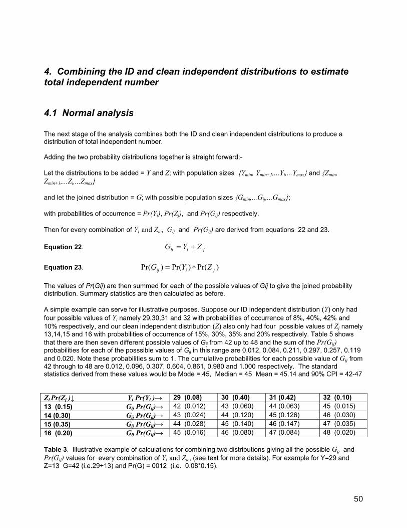
50

4. Combining the ID and clean independent distributions to estimate total independent number

4.1 Normal analysis The next stage of the analysis combines both the ID and clean independent distributions to produce a distribution of total independent number. Adding the two probability distributions together is straight forward:- Let the distributions to be added = Y and Z; with population sizes {Ymin, Ymin+1,...Yi,...Ymax} and {Zmin, Zmin+1,...Zi,...Zmax} and let the joined distribution = G; with possible population sizes {Gmin,...Gij,...Gmax}; with probabilities of occurrence = Pr(Yi), Pr(Zj), and Pr(Gij) respectively. Then for every combination of Yi and Zic, Gij and Pr(Gij) are derived from equations 22 and 23. Equation 22. jiij ZYG += Equation 23. )Pr()Pr()Pr( jiij ZYG ∗= The values of Pr(Gij) are then summed for each of the possible values of Gij to give the joined probability distribution. Summary statistics are then calculated as before. A simple example can serve for illustrative purposes. Suppose our ID independent distribution (Y) only had four possible values of Yi namely 29,30,31 and 32 with probabilities of occurrence of 8%, 40%, 42% and 10% respectively, and our clean independent distribution (Z) also only had four possible values of Zj namely 13,14,15 and 16 with probabilities of occurrence of 15%, 30%, 35% and 20% respectively. Table 5 shows that there are then seven different possible values of Gij from 42 up to 48 and the sum of the Pr(Gij) probabilities for each of the posssible values of Gij in this range are 0.012, 0.084, 0.211, 0.297, 0.257, 0.119 and 0.020. Note these probabilities sum to 1. The cumulative probabilities for each possible value of Gij from 42 through to 48 are 0.012, 0.096, 0.307, 0.604, 0.861, 0.980 and 1.000 respectively. The standard statistics derived from these values would be Mode = 45, Median = 45 Mean = 45.14 and 90% CPI = 42-47 Zi Pr(Zj )↓ Yi Pr(Yi )→ 29 (0.08) 30 (0.40) 31 (0.42) 32 (0.10) 13 (0.15) Gij Pr(Gij)→ 42 (0.012) 43 (0.060) 44 (0.063) 45 (0.015) 14 (0.30) Gij Pr(Gij)→ 43 (0.024) 44 (0.120) 45 (0.126) 46 (0.030) 15 (0.35) Gij Pr(Gij)→ 44 (0.028) 45 (0.140) 46 (0.147) 47 (0.035) 16 (0.20) Gij Pr(Gij)→ 45 (0.016) 46 (0.080) 47 (0.084) 48 (0.020) Table 3. Illustrative example of calculations for combining two distributions giving all the possible Gij and Pr(Gij) values for every combination of Yi and Zic, (see text for more details). For example for Y=29 and Z=13 G=42 (i.e.29+13) and Pr(G) = 0012 (i.e. 0.08*0.15).

51

4.2 Multi-area analysis The next stage of the analysis combines both the ID and clean independent distributions for that area to produce a distribution of total independent number for that area using the method outlined in section 4.1 above. The usual statistics are then extracted from this distribution to give area clean estimates and CPI levels. After each total independent estimate is produced it is added to a running total distribution of all the areas analysed so far. The standard method for combining distributions is once again used to add the latest distribution to the running total distribution. Once all areas have been processed the final running total distribution becomes the total clean independent distribution for the whole park. The usual statistics are then extracted from this distribution to give total park clean estimates and CPI levels.

5. ESTIMATION OF THE NUMBER OF DEPENDENTS RHINO 2.0 then uses bootstrapping algorithms to first estimate the number of Dependents of Identifiable Independents, and then secondly the number of dependents of Clean Independents. The two resulting dependent probability distributions are then combined (using the same method described above in section 4) to produce a total dependent distribution. Estimates and CPI levels are derived for each of these distributions as before.

5.1 Making up of Dependent number data set(s) prior to Bootstrapping In the case of Dependents of ID independents, RHINO makes a data set of the number of Dependents seen with each Identifiable Independent alive in the population at the end of the sampling period, the last time each indentifiable independent was seen. This allows the dependent population estimate to be as up to date as possible. For example Betty may not have had a calf for much of the sampling period, but she gives birth and is last seen with her calf near the end of the sampling period. The dependent number used in for Betty in this case would be 1 to reflect her current status. The sum of all these dependent numbers for all the identifiable independents is used to derive a minimum prior estimate of dependents of ID independents. With clean rhino we don’t know which of the sightings were last sightings, and so the dataset for dependents of clean rhino simply contains the dependent numbers seen in all clean independent sightings in the main run data set. In the case of black rhino, the number of dependents per independant rhino will either be a 0, 1, or very occasionally a 2.

5.2 Bootstrapping the calf number datasets RHINO uses a bootstrapping algorithm to estimate dependent population sizes for each of two possible independent population segments. These segments are :

• The Dependents of Identifiable Independents (ID only Dependent estimation) • The Dependents of Clean Independents (Clean only Dependent estimation).

Biological data frequently do not come from well known distributions such as the Normal distribution. In such cases the non-parametric bootstrap approach, developed by Efron (1979), uses a sample of the data themselves to estimate the shape of the parent distribution (Knox and Peet 1989). Bootstrapping is a computer-based method, which substitutes considerable amounts of computation in place of theoretical

52

analysis. The bootstrap method is a convenient technique for estimating the standard error of a parameter estimate that has complicated analytic properties (Buckland 1984). It also can be used for estimating confidence levels (Efron 1981). Although the basic idea is remarkably simple (Manly 1991) the bootstrap can non-parametrically routinely answer questions which are far too complicated for traditional statistical analysis (Efron & Tibshirani 1986, Efron 1981). Given the speed of modern PC’s computer intensive methods have become increasingly feasible. The bootstrap effectively gives the statistician a simple formula for any statistic, no matter how complicated (Efron & Tibshirani 1986). In bootstrapping, a large number of random samples, called bootstrapped samples, are randomly drawn with replacement from the original data sample. Each observation in the original sample has an equal chance of selection. In RHINO the sample of data is a list of the number of dependants seen with each independent animal. Therefore in each bootstrap sample some observations may be left out by chance, while others appear a number of times. This gives an empirical distribution of dependent number per adult. The bootstrap sample in this case is the same as a random sample of size S drawn with replacement from the actual sample of dependent numbers. RHINO sets the bootstrap sample size, S, at the largest independent population size (for the segment being estimated) where Pr(Ni) $ 0.001. The statistic of interest (which in this case is the total number of calves) is then calculated for each replicate bootstrap sample. The expected error in the bootstrapped statistics can then be examined by plotting the distribution of the bootstrap replicate values. It is tempting to set 90% confidence limits for a parameter by moving 1.645 standard errors in either direction from the mean. This relies on asymptotic normality and often performs well with large samples. In many cases however, this method gives a an actual confidence level that is far short of the actual level, and in some cases the confidence level for the parameter may include impossible values (Buckland 1984, Efron & Gong 1983, Zucchini & Channing 1986). Bootstrap methods can be used to produce approximate confidence intervals for sample statistics, but with a less secure theoretical foundation than for bootstrap measures of statistical error (Efron 1982, op.cit. Knox and Peet 1989). In practice, to produce approximate confidence intervals using bootstrapping requires a large number of bootstrap samples (Buckland 1984, Efron & Tibshirani 1986, Efron 1987). Empirical testing indicates one should take at least a 1000 bootstrap samples before the confidence levels stabilise (Buckland 1984; Efron & Tibrishani 1986). For this reason RHINO randomly draws a total of 1000 bootstrap samples of S dependent numbers. The advantage of Monte Carlo type non-parametric methods like the bootstrap is that they attempt to capture the correct symmetry and provide robust non-parametric confidence levels. The shape of the bootstrap distribution will help determine the shape of the confidence interval (Efron & Tibshirani 1986). The Dependent numbers are then totalled for each of the 1000 replicate bootstrap samples. The frequency distribution of these 1000 totals estimates the distribution of bootstrapped dependent population size {Bmin, Bmin+1,...Bi,...Bmax} given a population of Independents, S. There a number of ways of using the bootstrap to estimate approximate confidence levels (Efron & Gong 1983, Buckland 1984, Efron and Tibrishani 1986), but the simplest approach involves assuming that the bootstrap distribution approximates the sampling distribution of the statistic of interest (which in our case is the number of rhino calves). Confidence levels can then be approximated by taking the appropriate percentiles from the bootstrapped distribution (Manly 1991). For example, the 5% and 95% percentiles from the bootstrap distribution provide an estimate of the 90% confidence level. However, as s represents the maximum likely Independent population size, the bootstrapped distribution will almost certainly overestimate the true population size. The bootstrapped distribution of the Dependent population size therefore needs to be adjusted downwards before any measures of central tendencies or confidence levels are estimated.

53

5.3 Adjustment of the Bootstrapped distribution In each of the 2 possible bootstrap options, RHINO modifies:

• The bootstrapped probability distribution {Bmin, Bmin+1,..Bi...Bmax} using:

• The probability distribution of population size {Nmin, Nmin+1,..Nj...Nmax} for the chosen Independent population segment.

to arrive at the final estimated Dependent distribution. All possible Dependent population sizes (Dij) together with their probabilities are calculated for all possible combinations of Bi and Nj as derived using equations 24 and 25.

Equation 22. S

NBD j

iij ∗=

Where S = the bootstrap sample size for the dependent segment being estimated (set at the largest independent population size for the segment being estimated where Pr(Ni) $ 0.00001) Equation 23. )Pr()Pr()Pr( jiij NBD ∗= The values of Dij are then rounded off to the nearest integer. The probabilities for each integer value of Dij are then summed to give the adjusted distribution of dependants. In the case of dependents of ID animals the total number of dependents seen in the last sightings of each of the independent animals during sampling (provided that the animals were still in the population at the end of the period) gives a minimum prior estimate. In RHINO 2, probabilities for any values of Dij less than the prior minimum are added to the prior minimum. In the case of dependents of ID Independants, RHINO lets the data determine the minimum number of dependents (This is the total number of dependants seen with identifiable animals present at the end of the run. Only the most recent sightings of each identifiable independant are considered.) If it is known that you have at least X dependent animals, then this knowledge can be incorporated into the dependent population size estimation. If you supply a known minimum estimate the program checks to see if the data indicates there were more dependants. If so the known minimum from the data is greater than the supplied minimum this is used instead. In RHINO 1.0 it was found that overestimation biases were introduced whenever the minimum or supplied minimum dependent number was close to the actual population size. In such cases RHINO 1.0 would tend to upwardly bias population estimates of dependants. When using earlier versions of RHINO (1.0 and 1.1), it was possible to eliminate bias by supplying 1 as the minimum number of dependants. However, this invariably led to the generation of silly lower credible posterior intervals (i.e. lower than the known minimum). In such cases users faced a dilemma - either they could select an unbiased dependents of identifiable independants estimator, or produce better credible posterior intervals (but not both). These problems were caused

54

because the probabilities of the dependent population being less than the supplied minimum prior (x) were made equal to 0. All remaining probabilities were multiplied by a constant so that they summed to 1. The procedure was revised in RHINO 1.2 to produce both unbiased answers with sensible lower CPI values when the minimum number known is close to the actual dependent population. In RHINO 1.2 the measures of central tendency are calculated from the unadjusted clean probability distribution (without using any prior knowledge). This gives an unbiased estimate. All probabilities for clean dependant number < x (the minimum prior) are then transferred and added to the probability of the population = x . The probability of the population being < x has therefore again been set at 0, but by using a different method. Credible posterior intervals are then estimated from this revised posterior distribution. This modified method produces much improved posterior distributions and credible posterior interval estimates (compared to the earliest versions of RHINO (ver 1.0 and 1.1), whilst at the same time removing the source of bias in the calculation of dependent estimates (which occurred in RHINO 1.0 whenever the minimum prior was close to the true population).

5.4 Estimation of dependent number during a Multi-Area analysis The dependents of ID values included in an area’s dataset prior to bootstrapping are derived from the last sightings of all the independent animals deemed to be in the area for analysis purposes (i.e. ignoring other independent animals which were sighted in the are but whose sightings have been transferred to another area). The dependents of clean values in an area’s dataset prior to bootstrapping are derived from all the sightings of clean independents in the area. The XboundaryCF corrected ID independent posterior distribution and XboundaryCF corrected clean independent posterior distribution are used to adjust the derived bootstrapped distributions of the number of dependents of ID and clean independents respectively. The XboundaryCF is not applied to the dependent distributions themselves as the correction factor has already been applied to the distributions estimating the number of ID and clean independents and these corrected distributions are used in the dependent calculations. The resultant dependents of ID and dependents of clean distributions are combined using the method described in section 4 above to produce the total dependent distribution for each area. In the same manner as before running total distributions are calculated for each of the three dependent distributions with the final running total dependent distributions being used to give the total park dependent estimates.

6. TOTAL POPULATION ESTIMATION

6.1 Straight analysis The next stage of the analysis combines the total independent and total dependent distributions to produce a final total population distribution from which the standard statistics are extracted as before. Adding the two probability distributions together is straight forward and the method is as described in section 4 above.

55

6.2 Multi-Area analysis For each area analysis proceeds as above (section 6.1) In the same manner as before running total distributions are calculated the final running total distribution being used to give the total park population estimate.

Some performance characteristics of RHINO 2.0

1 Influence of mark-recapture sampling variability and estimation bias on clean estimation. The mark-recapture histories of your ID animals is a sample. If by chance you end up with a few more re-sightings than average in your sample, this will act to underestimate ID independent population size. RHINO assumes clean animals have the same mark-recapture histories (sighting frequencies) as ID independent animals, and so the precision of the ID independent estimate will also directly influence the precision of the clean independent estimate. Figures 16 and 17 show, at very low sampling intensities the positive bias introduced into the ID independent estimation process is carried forward into clean independent estimation as well.

2 Influence of binomial sampling error in sampling the proportion of total independent observations which are clean. Just as the total number of heads you will get after tossing a coin 100 times will vary, the number of clean sightings you record in your sample will also vary due to sampling chance. If by chance you record 23 clean sightings out of 100 observations, when in reality the clean proportion is 20%, this will act to bias the clean population estimate upwards. Sometimes the binomial sampling error and mark-recapture sampling error cancel each other out, while in other cases they may both work to bias estimates in the same direction.

3 Influence of sample size on clean and ID independent estimator bias and precison Using the multiple simulation option in RHINO 2.0 a total of 40,000 simulated datasets (and over 5 million simulated sightings) were generated and analysed for a simulated population set up with 45 ID independents and 45 clean independents. In order to examine the effect that sample size had on the results the number of observations in each simulated dataset was varied, from only 30 sightings/survey (mean sighting frequency/animal of only 0.33) up to 300 observations/survey (mean sighting frequency of 3.33 per animal). The replicate RHINO estimates were then sorted and the 5th and 95th percentile value in the data sets give the range within which the estimates could be expected to fall 90% of the time. The bootstrapped 90%

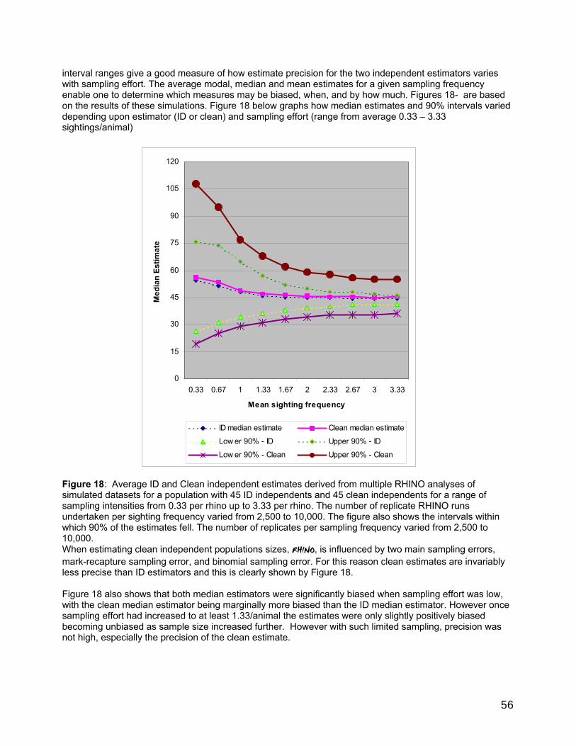
56

interval ranges give a good measure of how estimate precision for the two independent estimators varies with sampling effort. The average modal, median and mean estimates for a given sampling frequency enable one to determine which measures may be biased, when, and by how much. Figures 18- are based on the results of these simulations. Figure 18 below graphs how median estimates and 90% intervals varied depending upon estimator (ID or clean) and sampling effort (range from average 0.33 – 3.33 sightings/animal)

Figure 18: Average ID and Clean independent estimates derived from multiple RHINO analyses of simulated datasets for a population with 45 ID independents and 45 clean independents for a range of sampling intensities from 0.33 per rhino up to 3.33 per rhino. The number of replicate RHINO runs undertaken per sighting frequency varied from 2,500 to 10,000. The figure also shows the intervals within which 90% of the estimates fell. The number of replicates per sampling frequency varied from 2,500 to 10,000. When estimating clean independent populations sizes, RHINO, is influenced by two main sampling errors, mark-recapture sampling error, and binomial sampling error. For this reason clean estimates are invariably less precise than ID estimators and this is clearly shown by Figure 18. Figure 18 also shows that both median estimators were significantly biased when sampling effort was low, with the clean median estimator being marginally more biased than the ID median estimator. However once sampling effort had increased to at least 1.33/animal the estimates were only slightly positively biased becoming unbiased as sample size increased further. However with such limited sampling, precision was not high, especially the precision of the clean estimate.

0

15

30

45

60

75

90

105

120

0.33 0.67 1 1.33 1.67 2 2.33 2.67 3 3.33

Mean sighting frequency

Med

ian

Estim

ate

ID median estimate Clean median estimate

Low er 90% - ID Upper 90% - ID

Low er 90% - Clean Upper 90% - Clean

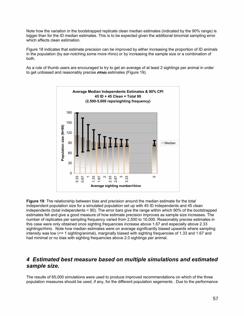
57

Note how the variation in the bootstrapped replicate clean median estimates (indicated by the 90% range) is bigger than for the ID median estimates. This is to be expected given the additional binomial sampling error which affects clean estimation. Figure 18 indicates that estimate precision can be improved by either increasing the proportion of ID animals in the population (by ear-notching some more rhino) or by increasing the sample size or a combination of both. As a rule of thumb users are encouraged to try to get an average of at least 2 sightings per animal in order to get unbiased and reasonably precise RHINO estimates (Figure 19).

Figure 19: The relationship between bias and precision around the median estimate for the total independent population size for a simulated population set up with 45 ID independents and 45 clean independents (total independents = 90). The error bars give the range within which 90% of the bootstrapped estimates fell and give a good measure of how estimate precision improves as sample size increases. The number of replicates per sampling frequency varied from 2,500 to 10,000. Reasonably precise estimates in this case were only obtained once sighting frequencies increase above 1.67 and especially above 2.33 sightings/rhino. Note how median estimates were on average significantly biased upwards where sampling intensity was low (<= 1 sighting/animal), marginally biased with sighting frequencies of 1.33 and 1.67 and had minimal or no bias with sighting frequencies above 2.0 sightings per animal.

4 Estimated best measure based on multiple simulations and estimated sample size. The results of 65,000 simulations were used to produce improved recommendations on which of the three population measures should be used, if any, for the different population segements . Due to the performance

Average Median Independents Estimates & 90% CPI 45 ID + 45 Clean = Total 90

(2,500-5,000 reps/sighting frequency)

0

30

60

90

120

150

180

0.33

0.67 1

1.33

1.67 2

2.33

2.67 3

3.33 5

Average sighting number/rhino

Popu

latio

n si

ze (N

=90)

Median

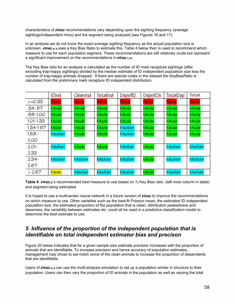
58

characteristics of RHINO recommendations vary depending upon the sighting frequency (average sightings/independent rhino) and the segment being analysed (see Figures 16 and 17). In an analysis we do not know the exact average sighting frequency as the actual population size is unknown. RHINO 2.0 uses a Key Bias Ratio to estimate this. Table 4 below then is used to recommend which measure to use for each population segment. These recommendations are still relatively crude but represent a significant improvement on the recommendations in RHINO 1.21. The Key Bias ratio for an analysis is calculated as the number of ID mark recapture sightings (after excluding trap-happy sightings) divided by the median estimate of ID independent population size less the number of trap-happy animals dropped. If there are special codes in the dataset the KeyBiasRatio is calculated from the preliminary mark recapture ID independent distribution. Table 4: RHINO 2’s recommended best measure to use based on 1) Key Bias ratio (left most column in table) and segment being estimated. It is hoped to use a multivariate neural network in a future version of RHINO to improve the recommendations on which measure to use. Other variables such as the best-fit Poisson mean, the estimated ID independent population size, the estimated proportion of the population that is clean, distribution peakedness and skewness, the variability between estimates etc. could all be used in a predictive classification model to determine the best estimate to use.

5 Influence of the proportion of the independent population that is identifiable on total independent estimator bias and precison Figure 20 below indicates that for a given sample size estimate precision increases with the proportion of animals that are identifiable. To increase precision and hence accuracy of population estimates, management may chose to ear-notch some of the clean animals to increase the proportion of idependents that are identifiable. Users of RHINO 2.0 can use the multi-analysis simulation to set up a population similar in structure to their population. Users can then vary the proportion of ID animals in the population as well as varying the total

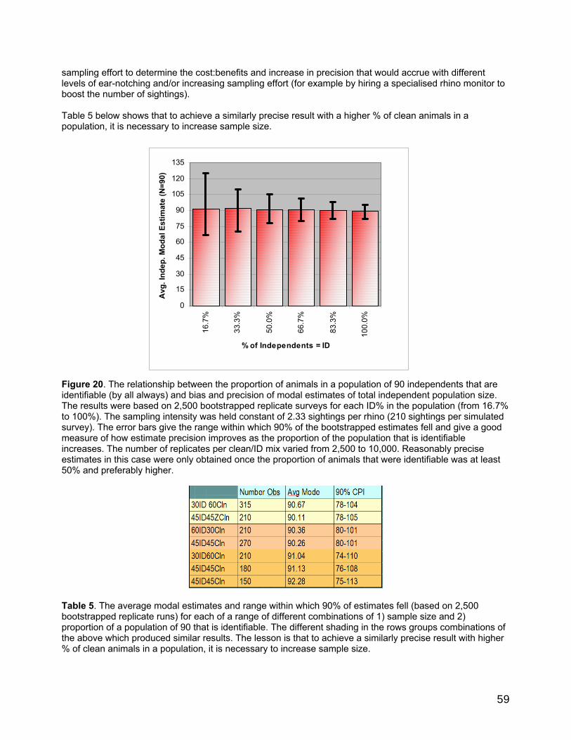
59

sampling effort to determine the cost:benefits and increase in precision that would accrue with different levels of ear-notching and/or increasing sampling effort (for example by hiring a specialised rhino monitor to boost the number of sightings). Table 5 below shows that to achieve a similarly precise result with a higher % of clean animals in a population, it is necessary to increase sample size. Figure 20. The relationship between the proportion of animals in a population of 90 independents that are identifiable (by all always) and bias and precision of modal estimates of total independent population size. The results were based on 2,500 bootstrapped replicate surveys for each ID% in the population (from 16.7% to 100%). The sampling intensity was held constant of 2.33 sightings per rhino (210 sightings per simulated survey). The error bars give the range within which 90% of the bootstrapped estimates fell and give a good measure of how estimate precision improves as the proportion of the population that is identifiable increases. The number of replicates per clean/ID mix varied from 2,500 to 10,000. Reasonably precise estimates in this case were only obtained once the proportion of animals that were identifiable was at least 50% and preferably higher.

Table 5. The average modal estimates and range within which 90% of estimates fell (based on 2,500 bootstrapped replicate runs) for each of a range of different combinations of 1) sample size and 2) proportion of a population of 90 that is identifiable. The different shading in the rows groups combinations of the above which produced similar results. The lesson is that to achieve a similarly precise result with higher % of clean animals in a population, it is necessary to increase sample size.

0

15

30

45

60

75

90

105

120

135

16.7

%

33.3

%

50.0

%

66.7

%

83.3

%

100.

0%

% of Independents = ID

Avg

. Ind

ep. M

odal

Est

imat

e (N

=90)

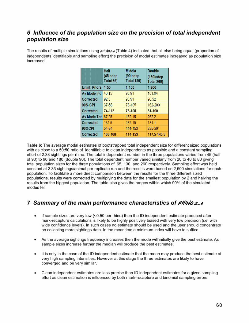
60

6 Influence of the population size on the precision of total independent population size The results of multiple simulations using RHINO2.0 (Table 4) indicated that all else being equal (proportion of independents identifiable and sampling effort) the precision of modal estimates increased as population size increased. Table 6: The average modal estimates of bootstrapped total independent size for different sized populations with as close to a 50:50 ratio of identifiable to clean independents as possible and a constant sampling effort of 2.33 sightings per rhino. The total independent number in the three populations varied from 45 (half of 90) to 90 and 180 (double 90). The total dependent number varied similarly from 20 to 40 to 80 giving total population sizes for the three populations of 65, 130, and 260 respectively. Sampling effort was held constant at 2.33 sightings/animal per replicate run and the results were based on 2,500 simulations for each population. To facilitate a more direct comparison between the results for the three different sized populations, results were corrected by multiplying the data for the smallest population by 2 and halving the results from the biggest population. The table also gives the ranges within which 90% of the simulated modes fell.

7 Summary of the main performance characteristics of RHINO 2..0

• If sample sizes are very low (<0.50 per rhino) then the ID independent estimate produced after mark-recapture calculations is likely to be highly positively biased with very low precision (i.e. with wide confidence levels). In such cases no estimate should be used and the user should concentrate on collecting more sightings data. In the meantime a minimum index will have to suffice.

• As the average sightings frequency increases then the mode will initially give the best estimate. As

sample sizes increase further the median will produce the best estimates.

• It is only in the case of the ID independent estimate that the mean may produce the best estimate at very high sampling intensities. However at this stage the three estimates are likely to have converged and be very similar.

• Clean independent estimates are less precise than ID independent estimates for a given sampling

effort as clean estimation is influenced by both mark-recapture and binomial sampling errors.

61

• To obtain a relatively unbiased or unbiased estimates of both ID independent and clean independent population sizes users should strive to achieve a mean sighting frequency for non trap-happy animals of at least 1.33 and preferably 2+.

• The higher the proportion of the population that are clean, the less precise, and at lower sampling

intensities the more biased the total independent estimates produced. Ear-notching which increases the proportion of the population that is identifiable will lead to more precise estimates for a given sample size. (Ear notching has other benefits such as increasing the sample size of known breeding females and allowing an improved assessment of population reproductive performance, as well as providing an opportunity to take some tissue samples, as well as fit transponders in the animals shoulder as well as horns. The latter could help identify horns later if recovered in an illegal bust, and shoulder transponders may help identify animals that have died and had their ears bitten off by scavenging hyenas.). Precision can also be increased by increasing sample size. The multi simulation option in RHINO 2.0 is a useful tool for determining the likely cost:benefits of ear notching more rhinos or temporarily hiring a rhino monitor to boost sample sizes.

• For a given sampling intensity the precision of estimates improves as population size increases.

Therefore to get a similar precision around your estimate when you have a smaller population you need either or a combination of a higher proportion of the population identifiable or a greater average sighting frequency.

To recap, the five key points to remember are … 1. The best measure estimating numbers varies depending on segment of population being estimated and sampling effort. 2. You need at least 1.33 sightings/rhino and preferably 2+ sightings/rhino 3. The bigger the size of the population the more precise the estimate, and lower the confidence levels (for a given sampling effort). 4. The higher the proportion of the independent population that is identifiable, the more precise the estimate and lower the confidence levels (for a given sampling effort) 5. The higher the sampling effort the less biased and more precise the estimate and lower the confidence levels

ACKNOWLEDGEMENTS

1 Development of the earlier versions of RHINO As RHINO 2.0 built upon earlier versions it is appropriate to acknowledge those involved with the development of earlier versions of the software as well. Walter Zucchini first developed a Bayesian analogue of the Schnabel census method for analysing sighting/re-sighting data collected on discrete surveys (Zucchini & Channing 1986). Leslie Underhill then produced a special case of the Zucchini method, to analyse sightings data collected one at a time (Underhill & Fraser 1989). The modifications to the basic Underhill method to deal with trap happy animals and special code animals were made by Richard Emslie.

62

Richard Emslie developed the methods to estimate clean population size. Keryn Adcock made useful suggestions on how to treat marked animals during the calculation of clean population sizes. Leslie Underhill and Berty van Hensbergen suggested that iterative area-happy subsetting could be used to deal with the problem of area happy data collection and this option was included in earlier versions of RHINO. However for the reasons outlined in this reference manual, this option has been dropped from RHINO 2.0 and replaced with a multi-area analysis option. The graphical approach to determining whether the assumption of equal catchability had been violated by trap-happy animals was developed by Richard Emslie. In the early days of RHINO development Keryn Adcock supplied much useful information on problems experienced when trying to identify trap-happy animals using real data sets. The adjusted bootstrapping approach (with data derived priors) used to estimate dependent population sizes was developed by Richard Emslie. He would like to thank Berty van Hensbergen, Keryn Adcock and Walter Zucchini for their valuable discussions which introduced him to bootstrapping. Neil Pendock recommended that maximum entropic informative priors should be used whenever possible. He suggested that Jaynes' transformation should be used to maximise entropy of informative priors. In practice this made little or no difference to the results and was dropped from RHINO 2.0. Richard Emslie did all the programming for earlier versions of RHINO (1.0, 1.1, 1.2 and 1.21) Berty van Hensbergen suggested that the minimum prior could perhaps be derived from the data to reduce the number of computations required in earlier versions of the software. With the speed of modern computers this is no longer an issue. The development of the original RHINO software was primarily sponsored by Ecoscot Consultancy Services with a little funding from WWF (South Africa), Total Oil, The Endangered Wildlife Trust and the then Natal Parks Board.

2 Development of RHINO 2.0 The rewriting and enhancing of RHINO 2.0 would not have taken place without the significant funding provided by the Italian-funded SADC Regional Programme for Rhino Conservation. The development and re-writing of RHINO2.0 from scratch was the work of a team made up of Richard Emslie, Rajan Amin and Kevin Davey. All concerned have put far more work into this project than they were paid for. The balance of funding (and extra time worked) has been provided by Richard Emslie and Ecoscot Consultancy Services, Raj Amin (Zoological Society of London) and Kevin Davey. Rajan Amin undertook some simulation modelling in Matlab to determine if the Emslie clean estimator was better than then Stead clean estimator. The results of this modelling indicated that the Emslie estimator should be retained in RHINO 2.0, and not replaced with a modified Stead estimator. Richard Emslie simplified the RHINO 1.21 equations for clean estimation to take into account that area-happy sampling was no longer an option for inclusion in RHINO 2.0 Rajan Amin and Richard Emslie ran the same datasets through RHINO 1.21 and RHINO 2.0 to ensure compatibility between previous RHINO versions (after allowing for any algorithm changes between versions and calculation differences (e.g rounding) between Paradox (used for earlier versions of RHINO) and Access (Used to program RHINO 2 ) and Matlab (used to test and debug some maths routines).

63

The basic algorithm for multi area analysis (including the cross boundary movement bias correction) in RHINO 2.0 was developed by Richard Emslie following extensive discussions with Rajan Amin and Kevin Davey. In all discussions on new approaches/algorithms to be used Rajan Amin acted as an excellent sounding board for any ideas by the original developer (Richard Emslie). Kevin Davey’s intelligent questions from time to time from the perspective of someone new to animal population estimation and rhino monitoring also improved the software. The idea of using a goodness of fit measure to automate selection of trap-happy animals in RHINO 2.0 was Richard Emslie’s, but the application of this would not have been possible without the programming skills of Rajan Amin and Kevin Davey. Rajan Amin developed the algorithms to calculate measures of skewness and peakedness. Fortunately for users of RHINO 2.0, the programming in the new version was not done by an amateur programmer. All the coding of mathematical algorithms in RHINO 2.0 was expertly done by Rajan Amin. All the front-end user interface and graph and report generation programming was done by Kevin Davey. The use of skilled programmers to write RHINO2.0 has made a significant difference to the mathematical efficiency and ease of use of the programme.The structure and interfacing together of the various routines in RHINO 2.0 was developed jointly by Raj Amin and Kevin Davey. Raj’s maths routines are now more efficient, and Kevin’s front end programming has made RHINO easier and more intuitive to use. RHINO 2.0 was developed in an interative fashion with each version received from the programmers (Raj and Kevin) being tested for bugs and problems by Richard. Problems and suggested solutions/fixes were then sent back to the programmers who then produced the next version. Planning, development and testing of the software was a team effort by Richard Emslie, Rajan Amin and Kevin Davey. This process was assisted by exchanges of detailed e-mails, and meetings in London, as well as in South Africa. A visit to Hluhluwe Research Centre in Hluhluwe-Imfolozi Park also assisted with the testing and further development of the software in the field. Owen Howison is thanked for his time and input during this visit. The Zoological Society of London and in particular Paul Pearce-Kelly and Raj Amin are thanked for often providing Richard Emslie with accommodation at London Zoo and a place to work. Ecoscot Consultancy Services sponsored some of the costs of the trip to South Africa by Rajan Amin and Kevin Davey. Lulama Fanayo, Sue van Rensburg and the field managers in Hluhluwe-Imfolozi Park are thanked for drawing attention to the potential overestimation bias problem caused by not including incomplete mortality records in RHINO run datasets. Based on the results of simulation modelling, Richard Emslie was able to advise on how to deal with such sightings in the interim. All users over the years are thanked for their feedback and sharing experiences. The simulation modelling and development of the statistical advisor was undertaken by Richard Emslie. The algorithms for the different simulation options in RHINO 2.0 were developed jointly by Richard Emslie, Raj Amin and Kevin Davey. The manuals were produced by Richard Emslie (any mistakes are his!). Derek Brown is thanked for permission to use his photograph of a black rhino in Great Fish River Reserve.

64

3. Last but not least

65

REFERENCES Adcock, K., Conway A. and Wills A.J. (1990). Annual black rhino status report to the Rhino Management Group for the period 1 April 1989 - 31 March 1990 for Hluhluwe-Umfolozi Game Reserve. 14pp unpublished confidential report. Brooks P.M. (1989) Conservation Plan for the black rhinoceros in South Africa, The TBVC states and SWA/Namibia (Rhino Management Group) Best, P.B. and Underhill, L.G. (1989) Estimating population size in Southern Right Whales Eubalaaena australis using naturally marked animals. Reports of the International Whaling Commission. Buckland S.T. (1984) Monte Carlo Confidence Intervals, Biometrics 40 pp 811-817 Burnham, K.P; Anderson D.R. and Laake, J.L. (1980) Estimation of density from line transect sampling of biological populations. Wildlife Monograph 72:1-202 Castledine B.J. (1981) A Bayesian analysis of multiple-recapture sampling for a closed population. Biometrika 68, pp 197-630. Chao, A. (1989) Estimating population size for sparse data in capture-recapture experiments. Biometrics 45, pp427-438. Craig, C.C. (1956). On the utilisation of marked specimens in estimating populations of insects. Biometrika 45, 343-359. Donoho D.L., Johnstone I.M., Hoch J.C. and Stern A.S. (19??) Maximum entropy and the nearly black object. JRSS-B, 54, 41-81 Du Feu, C.R., Hounsome, M.V. and Spence, I.M. (1983). A single-session mark/recapture method of population estimation. Ringing & Migr. 4, 211-226. Efron, B. (1979). Bootstrap methods: Another look at the jackknife. Ann. Statist. 7: 1-26. Efron, B. (1981). Censored data and the Bootstrap J.Am.Stat.Assoc. 76: 312-319. Efron, B. (1982). The jackknife, the bootstrap, and other resampling plans. SIAM Monograph 38. Efron, B. and Gong, Gail (1983). A Leisurely Look at the Bootstrap, the Jacknife, and Cross-Validation. The American Statistician Feb1983 Vol 37 Number 1 pp 36-48 Efron, B. and Tibshirani, R (1986). Bootstrap Methods for Standard Errors, Confidence Intervals, and Other Measures of Statistical Accuracy Statistical Science Vol 1 Number 1 pp 54-77 Efron, B. (1987). Better bootstrap confidence intervals. J. Amer. Statist. Assoc. 82: 171-185. Emslie Richard H. (1991) Status Report Summary 1990-91 Confidential Rhino Management Group publication (55pp) Emslie Richard H. (1991) RHINO version 1.0 - A population estimation analysis package designed for black rhinoceros in particular, but applicable to other species. In collaboration with Leslie G.Underhill, Berty (H) J. van Hensbergen, Keryn Adcock, and Walter Zucchini. Black Rhino Project 2000/Ecoscot Consultancy Services 68pages

66

Emslie Richard H. (1992) Value of regional black rhino status reporting - Paper presented at the 1992 IUCN SSC African Rhino Specialist Group meeting at Vic Falls, Zimbabwe November 1992; unpublished ARSG paper (7pp). Gazey, W.J. and Staley, M.J. (1986). Population estimation from mark/recapture experiments using a sequential Bayes algorithm. Ecology 67, 941-951. Hansen H.B. & Lindemann H. (1989) Black rhino identification in Pilanesberg National Park ; Bop Parks Internal Report Hansen H.B. & Lindemann H. (1990) Black rhino identification in Pilanesberg National Park - a follow up survey ; Bop Parks Internal Report Hansen H.B. & Lindemann H. (1991) Black rhino monitoring - Pilanesberg National Park ; Bop Parks Internal Report Hitchins, P.M. and Brooks, P.M. (1986). Preliminary report on the population size and trend (1973-1985) of the black rhinoceros in the Hluhluwe and Umfolozi Game Reserves, 1985. Natal Parks Board 13pp unpublished report Hitchins, P.M. (1986) Report on the population size and trend of the black rhinoceros in the central complex, 1985. 7 pp unpublished report Jaynes E.T (1968) Prior probabilities, IEE Trans. Systems Science and Cybernetics, SSC4 Johnson, Douglas H. (1989) An Empirical Bayes Approach to Analysing Recurring Animal Surveys. Ecology 70(4) pp945-952 Knox, R.G. and Peet, R.K. (1989). Bootstrapped ordination: a method for estimating sampling effects in indirect gradient analysis. Vegetatio 80, 153-165. Lawson, K., Apps, P. and Panagis, K. (1988). A new method for counting animals in small populations of recognisable individuals. Madoqua 15:4, 343-346 Lindemann Hanne, and Hansen Hans B. (1992) Black rhino identification in Pilanesberg National Park. ; Bop Parks Internal Report Manly, Bryan F.J. (1991) Randomization and Monte Carlo Methods in Biology. Chapman and Hall, 269pp. Pendock N, and Emslie R.H. (in prep) Counting Rhinos Rodrigues, J., Bolfarine, H. and Leite, J.G. (1988) A Bayesian analysis in closed animal populations from capture recapture experiments with trap response. Communications in Statistics: Simulation 17, pp 407-430. Sandwith T.S., Emslie R.H. & Adcock K. (1988) Black rhino monitoring programme - HGR and UGR Natal Parks Board/Black Rhino 2000 report pp6 Schnabel, Z.E. (1938) The estimation of the total fish population of a lake. Am. Math. Mon. 45, 348-352. Stead Gareth (1991) Estimating the population size of the black rhinoceros in the Hluhluwe-Umfolozi Game Reserve using Bayesian Techniques BSc Honours Thesis, Actuarial Science, Department of Statistics, University of Cape Town 89pp. Underhill, L.G. (1989). Bayesian estimation of the size of closed populations. 28pp unpublished manuscript.

67

Underhill, L.G. and Fraser, M.W. (1989). Bayesian estimate of the number of Malachite sunbirds (Nectarinia famosa) feeding at an isolated and transient nectar resource. J. Field Ornithol. 60(3). White Gary C., Anderson David,R., Burnham Kenneth P., and Otis David L. (1982) Capture-Recapture and Removal Methods for Sampling Closed Populations. Los Alamos National Laboratory, New Mexico, Publication LA-8787-NERP 235pp. Wolf T.P (1992) The November 1991 black rhino survey - Itala Game Reserve. 9pp Natal Parks Board report. Zucchini, W. (1992) Two steps towards our new goals - 1992 South African Statistical Association Presidential Address, S.A.Statistical Assoc. Newsletter December 1992 pp 5-12 Zucchini, W. and Channing, A. (1986). Bayesian estimation of animal abundance in small populations using capture and recapture information. S. Afr. J. Sci. 82, 137-140.

GLOSSARY OF UNFAMILIAR TERMS OR TERMS USED IN A SPECIFIC WAY BY RHINO

Clean In RHINO this term refers to animals which have no obvious distinguishing features (such as ear tears and ear notches) which enable them to be individually identified by all trained observers every time they see them . Some animals may be identifiable only to experienced key observers on the basis of more subtle or harder to record features (e.g. horn configurations) and or on the basis of photos. In such cases, although such animals may be identifiable as an individual, they will not always be identified by all observers in a monitoring programme. As one of the assumptions of mark-recapture programmes is that marked animals stay marked and can always be identified, such sightings fail the always by all test and so are treated as clean sightings by RHINO. However information on the number of clean rhino that can be identified sometimes by key observers (on more subtle/harder to record features or from photos) can be used by RHINO.

Marked The term refers to making a clean animal identifiable during an estimation period. (In the case of black rhino, clean animals can be darted using a helicopter and ear notched by a follow up ground crew.) Any sightings of marked animals before they were marked will have been recorded as clean. Ringing all birds caught in a mist net does not constitute marking as the birds are never recorded as clean. For analysis purposes all birds are identifiable from their first observation. Only animals that could have been recorded as clean before they are made identifiable are considered as having been marked.

68

Section and Area This is a database field that lists the region in which an animal was observed. In the case of black rhino, section may refer to different management regions in a large Game Reserve or National Park. RHINO allows sighting location to be classified as both Section and Area. The latter term here is used to refer to different areas or regions in a Park which may have been sampled at different intensities (area-happy data collection). The variable Area just provides users with an alternative way to subdivide a park for a Multi-Area analysis run

Independents and Dependents The term independent refers to animals that are statistically independent and are normally are on their own, or have one or more dependent offspring with them. The term dependent refers to animals that are not included directly in the mark-recapture analyses as they are attached to their mothers. In this case they are not statistically independent. In the case of black rhino all F aged adults and E aged sub-adults are independent and have left their mothers. However A-D aged calves less than 3½ + years old that are still attached to their mothers are treated as dependent animals. In the case of black rhinos calves normally leave their mothers by the time they are aged 3½ years old. However, it has been noted that young males occasionally return to spend some time with their mothers after becoming independent. In such cases, these animals should be treated as independant.

Non–Active records and Special codes Special codes are 1 or 2 letter codes which are sometimes entered in a Special Code field in the input database to mark records of introductions, removals, deaths, marking (i.e. ear-notching), or changes in status when identifiable dependents leave their mothers and become indentifiable independents. Special codes are used to inform RHINO of changes in size of any of the population segements. Special code records are not used to iteratively recalculate and update the posterior probabilities in the mark-recapture calculations and are therefore termed non-active records. These records are either used to shift the posterior distribution up or down, or alter the running total of the number of different individuals seen during the run which is used in subsequent mark-recapture analysis of active records.

Active records The term active record refers to records which are used in the mark-recapture calculations (equations 1 and 2). The special codes field is blank for these records. Active clean records refer to clean observations without special codes. Accuracy Accuracy refers to the closeness of a population estimate to the true population size and therefore monitoring programmes strive to produce accurate results. Accuracy is a function of both estimate bias and precision. To routinely produce accurate estimates a monitoring programme needs to be unbiased and precise.

69

Bias When the mean of a set of replicate estimates is equal to the true population size the method is said to be unbiased. If on the other hand the average estimate is lower or higher than the true population size the estimate is said to be biased. The direction of bias will determine whether estimates will on average be under or over estimates. Provided that bias operates in a consistent direction, and a monitoring technique is precise enough, then it can still be used to monitor trends in numbers. If the bias of a technique varies over time and with conditions, such a technique is of limited use for monitoring unless the nature and extent of the bias is predictable allowing different estimates to be individually bias corrected so that they can be compared. In order to estimate absolute population sizes and obtain accurate estimates of animal densities (important for biological management offtake decision-making) a monitoring technique needs to be unbiased. In some cases it is possible to apply a correction to account for bias and return an unbiased answer.

Precision Precision refers to the degree of variation between replicate estimates. A precise method will produce similar estimates when replicated. By way of contrast, different replicates using an imprecise method may produce estimates that differ substantially. The credible posterior intervals or confidence levels around an estimate indicate its likely precision. To be useful for monitoring trends in population size, a monitoring technique needs to be reasonably precise. If a monitoring method is imprecise then one cannot have any confidence that observed differences between estimates reflect real changes in population status due to the high chance of obtaining such differences as a result of sampling chance.