revisiting the theory of stability of stationary linear large-scale systems
TRANSCRIPT

REVISITING THE THEORY OF STABILITY OF STATIONARY LINEAR LARGE-SCALE
SYSTEMS
À.À. Martynyuk1
and R. V. Mullazhonov2
Linear autonomous large-scale systems are studied in the context with the generalized transposition of
the matrix and the structure of the system. New stability conditions are established with the help of a
matrix-valued Lyapunov function
Keywords: linear large-scale system, generalized transposition, stability, matrix-valued Lyapunov function
Introduction. The stability of linear large-scale systems in the context with their structure was analyzed in the
monograph [9] where there is an extensive bibliography. In [3], the operation of generalized transposition was proposed (cf. [1,
2, 10]), which allows us to classify the structures of a linear large-scale system.
In this paper we will analyze linear large-scale system for stability based on two possible decompositions along the
vertical and horizontal axes of symmetry and into balanced subsystems.
1. Preliminaries. Let A be an n n× matrix, and AT
, A⊥
, and A0
be the transposes of the matrix with respect to its main
diagonal, secondary diagonal, and center, respectively, (see [3] and the references therein). Consider the following systems:
�x Ax= , (1)
�x A xT= , (2)
�x A x= ⊥, (3)
�x A x= 0, (4)
where x x x= ( ,1 2
,� , )x Rn
T n∈ .
The following statement is true.
Theorem 1. If the equilibrium state of system (1) is stable (asymptotically stable) or unstable, then the equilibrium state
of systems (2), (3), and (4) is also stable (asymptotically stable) or unstable, respectively.
Proof. From the properties of matrix transposes (see [5]) it follows that
| | | | | | | |A E A E A E A ET− = − = − = −⊥λ λ λ λ0
,
i.e., the roots of the characteristic equations for the matrices A, AT
, A⊥
, and A0
are identical. This proves Theorem 1.
Example. For the matrix A =−
−− −
⎛
⎝
⎜⎜⎜
⎞
⎠
⎟⎟⎟
1 1 0
2 3 3
2 0 4
we have
International Applied Mechanics, Vol. 48, No. 1, January, 2012
1063-7095/12/4801-0101 ©2012 Springer Science+Business Media, Inc. 101
1S. P. Timoshenko Institute of Mechanics, National Academy of Sciences of Ukraine, 3 Nesterova St., Kyiv, Ukraine
03057, e-mail: [email protected] State University, 129 Universitetskaya St., Andijan, Uzbekistan 710000;
e-mail: [email protected]. Translated from Prikladnaya Mekhanika, Vol. 48, No. 1, pp. 121–132, January–February 2012.
Original article submitted April 26, 2010.

A AT =
− −−
−
⎛
⎝
⎜⎜⎜
⎞
⎠
⎟⎟⎟
=−
−− −
⎛
⎝
⎜⎜⎜
⎞
⎠
⊥1 2 2
1 3 0
0 3 4
4 3 0
0 3 1
2 2 4
,
⎟⎟⎟
=− −
−−
⎛
⎝
⎜⎜⎜
⎞
⎠
⎟⎟⎟
, A0
4 0 2
3 3 2
0 1 1
.
In all cases, the characteristic equation has the formλ λ λ3 28 17 10 0+ + + = and its roots areλ
11= − ,λ
22= − ,λ
35= − , i.e.,
the equilibrium state is asymptotically stable.
Corollary 1. If the matrix A in Theorem 1 is orthogonal with respect to the main (secondary) diagonal or center, then the
equilibrium state of the system
�x A x= −1(5)
is also stable (asymptotically stable) or unstable, respectively.
Indeed, if the matrix A is orthogonal with respect to the main (secondary) diagonal or center, then A AT = −1
, A A⊥ −= 1
,
A A0 1= −
, respectively, by the definition of orthogonal matrix, and Corollary 1 follows from Theorem 1.
Theorem 2. Consider the following Lyapunov function for system (1):
ϑ =( )x x PxT
, (6)
where P is a positive definite matrix symmetric with respect to the main diagonal or center. If the matrix
P H P PH1
1 1= =− −(7)
is positive definite, then the stability (asymptotic stability) or instability of the equilibrium state of system (1) means that the
equilibrium state of the following system is stable (asymptotically stable) or unstable, respectively:
�x HAx= , (8)
where H is a positive definite, nonsingular matrix symmetric with respect to the main diagonal or center.
Proof. We choose the following Lyapunov function for system (8):
ϑ =1 1
( )x x P xT
. (9)
Since the matrix P1
is positive definite by Theorem 2, function (9) is positive definite as well. The total derivative of
function (9) along the solutions of (8) has the form
�
( ) � � [( ) ]ϑ = + = +1 1 1 1 1
x x P x x P x x HA P P HA xT T T T
= + = +− −x A H H P PH HA x x A P PA x
T T T T T( ) ( )
1 1.
Then the functions (�
( ))ϑ1 8
x and (�
( ))ϑ x1
are either both positive definite or both negative definite, which proves Theorem 2.
Example. Let the matrix À in system (1) have the form
A =−
−⎛⎝⎜ ⎞
⎠⎟
1 1
2 3.
Then the Lyapunov function ϑ =( )x x ExT
, where E is a unit matrix, may be chosen as a candidate for system (1).
Consider the following nonsingular positive definite matrix symmetric with respect to the main diagonal:
H
h h
h hH
H
h h
h h=
⎛
⎝⎜⎜
⎞
⎠⎟⎟ =
−−
⎛
⎝⎜⎜
⎞−11 12
21 22
1 22 12
12 11
1,
| | ⎠⎟⎟
and the following system
102

� , �x HAx x
h h h h
h h h h= =
− + −− + −
⎛
⎝⎜⎜
⎞
⎠11 12 11 12
12 22 11 22
2 3
2 3⎟⎟ , (10)
where x x x RT= ∈( , )
1 2
2. Based on Theorem 2, we will use the following Lyapunov function for system (10):
ϑ = =−
−⎛
⎝⎜⎜
⎞
⎠⎟⎟−
1
1 22 12
12 11
1( )
| |x x H x x
H
h h
h hx
T T. (11)
Its total derivative along the solutions of (10) has the form
�
( )ϑ =−
−⎛⎝⎜ ⎞
⎠⎟
1
2 3
3 6x .
Thus, for the equilibrium state of system (10) to be asymptotically stable, it is sufficient that h i h h hii
> = >0 1 2 011 22 12
2, , ; – .
Theorem 2′. Let function (6) be a candidate Lyapunov function for system (1) and let there exist a positive definite
matrix
P HP PH1
= = , (7′)
where H is a positive definite, nonsingular matrix symmetric with respect to the main diagonal or center. Then the stability
(asymptotic stability) or instability of the equilibrium state of system (1) means that the equilibrium state of the following system
is stable (asymptotically stable) or unstable, respectively:
�x H Ax= −1. (8′)
The proof of Theorem 2′ is similar to the proof of Theorem 2.
Remark. If P E= in Theorem 2 (Theorem 2′), then Theorem 2 (Theorem 2′) remains valid when P H1
1= −( )P H
1= .
Theorem 3. Let ϑ =( )x x ExT
be a candidate Lyapunov function for the system
�x A x=0
, (12)
where x Rn∈ , A R
n n
0∈ ×
; E is a unit matrix of order n; H H Hm1 2
, , ,� are positive definite, nonsingular, nth-order matrices
symmetric with respect to the main diagonal or center.
Then the stability (asymptotic stability) or instability of the equilibrium state of system (12) means that the equilibrium
state of the following system is stable (asymptotically stable) or unstable, respectively:
�x Ax= (13)
A Ai
i
m
i=
⎛
⎝⎜⎜ =
∑α1
or A Ai
i
m
i=
=∑α
1
*, A H A
i i=
0, A H A
i i
* = −1
0, α
ii m≥ =0 1 2, , , ,� , ≠
⎞
⎠⎟⎟=
∑i
m
1
0 .
Proof. Theorem 3 follows from Theorems 2 and 2′.If A A
k j< , k j, ,= 1 2,� ,n, k j≠ , and α α
k j+ = 1, and α
i= 0, i k≠ , i j≠ , in Theorem 3, then the matrix À is such that
A A Ak j
≤ ≤ . (14)
Let us now analyze the stability of the equilibrium state of system (1) subject to some constraints. Let the matrix À in
system (1) be symmetric with respect to the matrix center. It is possible to decompose system (1) along the vertical and horizontal
axes of symmetry or into balanced subsystems.
2. Decomposition along the Axes of Symmetry. After decomposition along the vertical and horizontal axes, system
(1) becomes
103

�y A y B z= +1 1
, �z B y A z= +1
0
1
0, (15)
if n k= 2 , the free subsystems being
�y A y=1
, (16)
�z A z=1
0, (17)
�y A y a x B zk
= + ++1 2 1 1,
� ( ),
x a y a x a zk
T
k k k
T
+ + + += + +1 1 1 1 1 1
0,
�z B y a x A zk
= + ++1
0
2
0
1 1
0, (18)
if n k= +2 1, the free subsystem being (16), (17), and
�
,x a x
k k k k+ + + +=1 1 1 1
, (19)
where A1
and B1
are k k× matrices; A1
0and B
1
0are their transposes with respect to the matrix center, respectively,
a a a a a a ak k k k
T
k k k k1 1 1 1 2 1 2 1 2 1 3= =+ + + + + + +( , , ) , ( , ,
, , , , ,� � , )
,a
k n
T
+1,
y x x x z x x x x y x zk
T
k k n
T T
k
T= = =+ + +( , , , ) , ( , , , ) , ( , , )1 2 2 3 1
� �
T.
For system (15) and subsystems (16), (17), we choose a matrix-valued function
U y z
y y z
y z z1
11 12
21 2212 2
( , )
( ) ( , )
( , ) ( )=
ϑ ϑϑ ϑ
⎛
⎝⎜⎜
⎞
⎠⎟⎟ ϑ = ϑ( )
1, (20)
with elements
ϑ =11 1
( )y y P yT
, ϑ =22 1
0( )z z P z
T, ϑ = ϑ =
12 21 2( , ) ( , )y z y z y P z
T, (21)
which satisfy the following inequalities (see [5] and the references therein):
a) λ λm M y
kP y v y P y y N R( ) | | | | ( ) ( )| | | | ,
1
2
11 1
2≤ ≤ ∀ ∈ ⊆ ,
b) λ λm M z
kP z v z P z z N R( ) | | | | ( ) ( )| | | | ,
1
0 2
22 1
0 2≤ ≤ ∀ ∈ ⊆ ,
c) − ≤ ≤λ λm
T
M
TP P y z v y z P P y
1 2
2 2 12
1 2
2 2
/ /( ) | | | | | | | | ( , ) ( )| | | | | | | |z , (22)
for all ( , )y z N N Ry z
k k∈ × ⊆ ×, where P P
1 1
0, are positive definite matrices symmetric with respect to the main diagonal or
matrix center, P2
is a constant matrix, all the matrices being of order k; λm
( )⋅ and λM
( )⋅ are the minimum and maximum
eigenvalues of the matrices P1
and P1
0, respectively; λ
M
TP P
1 2
2 2
/( ) is the norm of the matrix P
2. Note that λ λ
m mP P( ) ( )
1 1
0= and
λ λM M
P P( ) ( )1 1
0= .
The scalar function
v y z U y zT
1 1( , ) ( , )= η η , (23)
where ηT = ( , )1 1 , satisfies the two-sided inequality
u A u v y z u A uT T
1 1 1 1 1 1 1≤ ≤( , ) , ∀ ( , )y z N N R
y z
k k∈ × ⊆ ×, (24)
104
where u y zT = (| | | | , | | | | );
AP P P
P P P
m M
T
M
T
m1
1
1 2
2 2
1 2
2 2 1
=−
−
⎛
⎝⎜⎜
⎞
⎠⎟⎟
λ λλ λ
( ) ( )
( ) ( )
/
/, A
P P P
P P P
m M
T
M
T
m
1
1
1 2
2 2
1 2
2 2 1
=−
−
⎛
⎝⎜⎜
⎞
⎠⎟⎟
λ λλ λ
( ) ( )
( ) ( )
/
/.
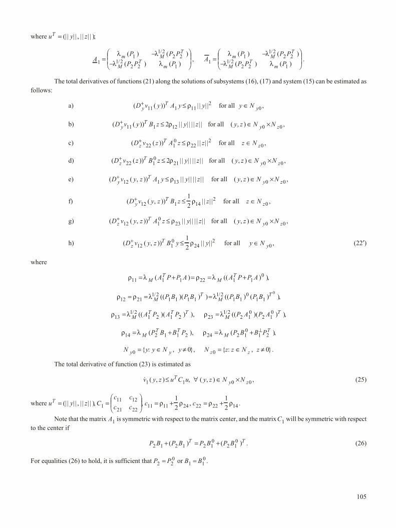
The total derivatives of functions (21) along the solutions of subsystems (16), (17) and system (15) can be estimated as
follows:
à) ( ( )) | | | |D v y A y yy
T+ ≤11 1 11
2ρ for all y Ny
∈0
,
b) ( ( )) | | | | | | | |D v y B z y zy
T+ ≤11 1 12
2ρ for all ( , )y z N Ny z
∈ ×0 0
,
c) ( ( )) | | | |D v z A z zz
T+ ≤22 1
0
22
2ρ for all z Nz
∈0
,
d) ( ( )) | | | | | | | |D v z B z y zz
T+ ≤22 1
0
212ρ for all ( , )y z N N
y z∈ ×
0 0,
e) ( ( , )) | | | | | | | |D v y z A y y zy
T+ ≤12 1 13
ρ for all ( , )y z N Ny z
∈ ×0 0
,
f) ( ( , )) | | | |D v y z B z zy
T+ ≤12 1 14
21
2ρ for all z N
z∈
0,
g) ( ( , )) | | | | | | | |D v y z A z y zz
T+ ≤12 1
0
23ρ for all ( , )y z N N
y z∈ ×
0 0,
h) ( ( , )) | | | |D v y z B y yz
T+ ≤12 1
0
24
21
2ρ for all y N
y∈
0, (22′)
where
ρ λ ρ λ11 1 1 22 1 1
0= + = = +M
T
M
TA P P A A P P A( ) (( ) ),
ρ ρ λ λ12 21
1 2
1 1 1 1
1 2
1 1
0
1 1
0
= = =M
T
M
TP B P B P B P B
/ /(( )( ) ) (( ) ( ) ),
ρ λ ρ λ13
1 2
1 2 1 2 23
1 2
2 1
0
2 1
0= =M
T T T
MA P A P P A P A
/ /(( )( ) ), (( )( ) )
T,
ρ λ ρ λ14 2 1 1 2 24 2 1
0
1 2= + = + ⊥
M
T T
M
TP B B P P B B P( ), ( ),
N y y N y N z z N zy y z z0 0
0 0= ∈ ≠ = ∈ ≠{ : , }, { : , }.
The total derivative of function (23) is estimated as
� ( , )v y z u C uT
1 1≤ , ∀ ( , )y z N N
y z∈ ×
0 0, (25)
where u y zT = (| | | | , | | | | ), C
c c
c c1
11 12
21 22
=⎛
⎝⎜⎜
⎞
⎠⎟⎟, c
11 11 24
1
2= +ρ ρ , c
22 22 14
1
2= +ρ ρ .
Note that the matrix A1
is symmetric with respect to the matrix center, and the matrixC1
will be symmetric with respect
to the center if
P B P B P B P BT T
2 1 2 1 2 1
0
2 1
0+ = +( ) ( ) . (26)
For equalities (26) to hold, it is sufficient that P P2 2
0= or B B1 1
0= .
105
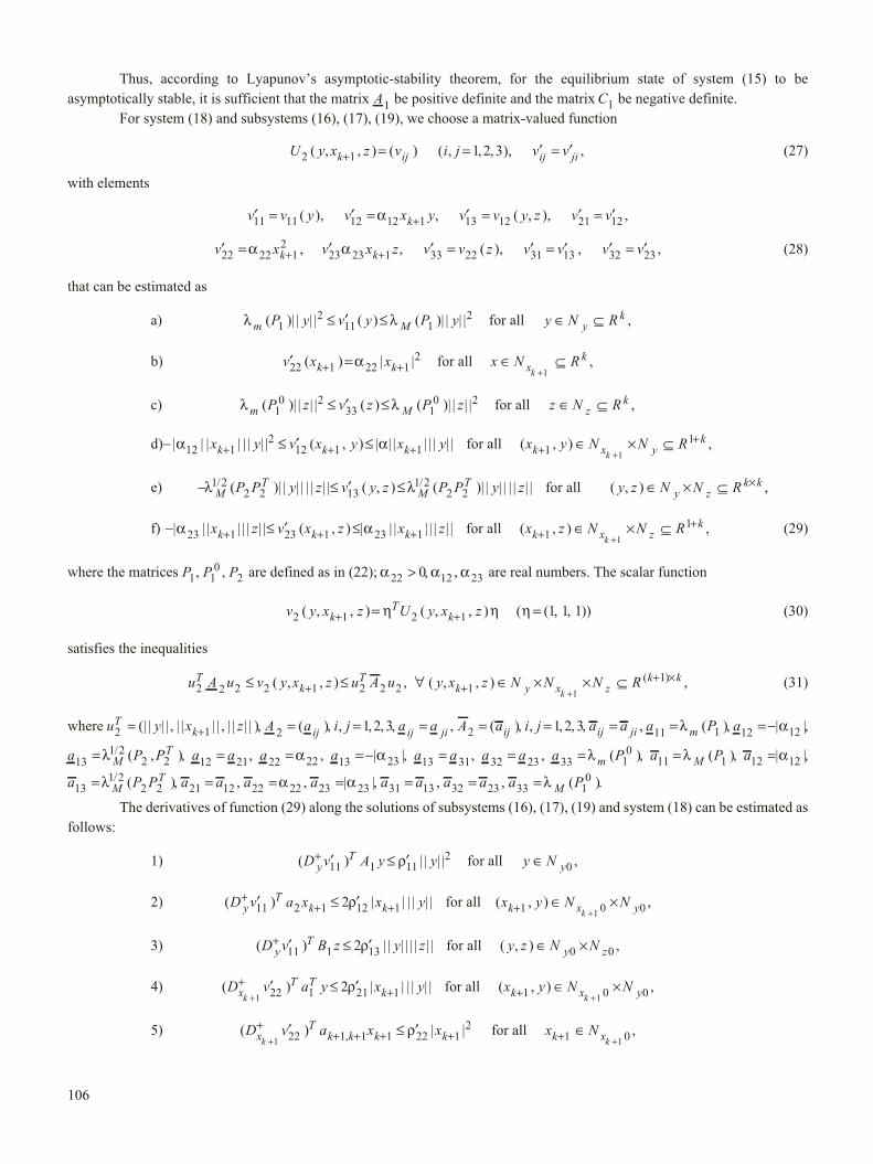
Thus, according to Lyapunov’s asymptotic-stability theorem, for the equilibrium state of system (15) to be
asymptotically stable, it is sufficient that the matrix A1
be positive definite and the matrix C1
be negative definite.
For system (18) and subsystems (16), (17), (19), we choose a matrix-valued function
U y x z v i j v vk ij ij ji2 1
1 2 3( , , ) ( ) ( , , , ),+ = = ′ = ′ , (27)
with elements
′ = ′ = ′ = ′ = ′+v v y v x y v v y z v vk11 11 12 12 1 13 12 21 12
( ), , ( , ),α ,
′ = ′ ′ = ′ = ′ ′+ +v x v x z v v z v vk k22 22 1
2
23 23 1 33 22 31 13α α, , ( ), , v v
32 23= ′ , (28)
that can be estimated as
à) λ λm M
P y v y P y( )| | | | ( ) ( )| | | |1
2
11 1
2≤ ′ ≤ for all y N Ry
k∈ ⊆ ,
b) ′ =+ +v x xk k22 1 22 1
2( ) | |α for all x N R
x
k
k
∈ ⊆+1
,
c) λ λm M
P z v z P z( )| | | | ( ) ( )| | | |1
0 2
33 1
0 2≤ ′ ≤ for all z N Rz
k∈ ⊆ ,
d)− ≤ ′ ≤+ + +| | | | | | | | ( , ) | | | | | | | |α α12 1
2
12 1 1x y v x y x y
k k kfor all ( , )x y N N R
k x y
k
k+
+∈ × ⊆+1
1
1
,
e) − ≤ ′ ≤λ λM
T
M
TP P y z v y z P P y
1 2
2 2 13
1 2
2 2
/ /( )| | | | | | | | ( , ) ( )| | | | | | | |z for all ( , )y z N N R
y z
k k∈ × ⊆ ×,
f) − ≤ ′ ≤+ + +| | | | | | | | ( , ) | | | | | | | |α α23 1 23 1 23 1
x z v x z x zk k k
for all ( , )x z N N Rk x z
k
k+
+∈ × ⊆+1
1
1
, (29)
where the matrices P1, P
1
0, P
2are defined as in (22); α
220> , α
12, α
23are real numbers. The scalar function
v y x z U y x zk
T
k2 1 2 1( , , ) ( , , )+ += η η ( ( , , ))η = 1 1 1 (30)
satisfies the inequalities
u A u v y x z u A uT
k
T
2 2 2 2 1 2 2 2≤ ≤+( , , ) , ∀ ( , , )
( )y x z N N N R
k y x z
k k
k+
+ ×∈ × × ⊆+1
1
1
, (31)
where u y x zT
k2 1= +(| | | | , | | | | , | | | | ), A a
ij2= ( ), i j, , ,= 1 2 3, a a
ij ji= , A a
ij2= ( ), i j, , ,= 1 2 3, a a
ij ji= , a P
m11 1= λ ( ), a
12 12= −| |α ,
a P PM
T
13
1 2
2 2= λ /
( , ), a a12 21
= , a22 22
= α , a13 23
= −| |α , a a13 31
= , a a32 23
= , a Pm33 1
0= λ ( ), a PM11 1
= λ ( ), a12 12
=| |α ,
a P PM
T
13
1 2
2 2= λ /
( ), a a21 12
= , a22 22
= α , a23 23
=| |α , a a31 13
= , a a32 23
= , a PM33 1
0= λ ( ).
The derivatives of function (29) along the solutions of subsystems (16), (17), (19) and system (18) can be estimated as
follows:
1) ( ) | | | |D v A y yy
T+ ′ ≤ ′11 1 11
2ρ for all y Ny
∈0
,
2) ( ) | | | | | |D v a x x yy
T
k k
++ +′ ≤ ′
11 2 1 12 12ρ for all ( , )x y N N
k x yk
+ ∈ ×+1 0 0
1
,
3) ( ) | | | | | | | |D v B z y zy
T+ ′ ≤ ′11 1 13
2ρ for all ( , )y z N Ny z
∈ ×0 0
,
4) ( ) | | | | | |D v a y x yx
T T
kk +
++′ ≤ ′
122 1 21 1
2ρ for all ( , )x y N Nk x y
k+ ∈ ×
+1 0 01
,
5) ( ) | |,
D v a x xx
T
k k k kk +
++ + + +′ ≤ ′
122 1 1 1 22 1
2ρ for all x Nk x
k+ ∈
+1 01
,
106

6) ( ) ( ) | | | | | |D v a z x zx
T T
kk +
++′ ≤ ′
122 1
0
23 12ρ for all ( , )x z N N
k x zk
+ ∈ ×+1 0 0
1
,
7) ( ) | | | | | | | |D v B y y zz
T+ ′ ≤ ′33 1
0
312ρ for all ( , )y z N N
y z∈ ×
0 0,
8) ( ) | | | | | |D v a x x zz
T
k k
++ +′ ≤ ′
33 2
0
1 23 12ρ for all ( , )x z N N
k x zk
+ ∈ ×+1 0 0
1
,
9) ( ) | | | |D v A z zz
T+ ′ ≤ ′33 1
0
33
2ρ for all z Nz
∈0
,
10) ( ) | | | |D v a y yx
T T
k +
+ ′ ≤ ′1
12 1 14
2ρ for all y Ny
∈0
,
11) ( ) | | | | | |,
D v a x x yx
T
k k k kk +
++ + + +′ ≤ ′
112 1 1 1 15 1
ρ for all ( , )x y N Nk x y
k+ ∈ ×
+1 0 01
,
12) ( ) ( ) | | | | | | | |D v a z y zx
T T
k +
+ ′ ≤ ′1
12 1
0
16ρ for all ( , )y z N N
y z∈ ×
0 0,
13) ( ) | | | | | |D v A y x yy
T
k
++′ ≤ ′
12 1 17 1ρ for all ( , )x y N N
k x yk
+ ∈ ×+1 0 0
1
,
14) ( ) | | | |D v a x xy
T
k k
++ +′ ≤ ′
12 2 1 18 1
2ρ for all x Nk x
k+ ∈
+1 01
,
15) ( ) | | | | | |D v B z x zy
T
k
++′ ≤ ′
12 1 19 1ρ for all ( , )x z N N
k x zk
+ ∈ ×+1 0 0
1
,
16) ( ) | | | | | | | |D v A y y zy
T+ ′ ≤ ′13 1 24
ρ for all ( , )y z N Ny z
∈ ×0 0
,
17) ( ) | | | | | |D v a x x zy
T
k k
++ +′ ≤ ′
13 2 1 25 1ρ for all ( , )x z N N
k x zk
+ ∈ ×+1 0 0
1
,
18) ( ) | | | |D v B z zy
T+ ′ ≤ ′13 1 26
2ρ for all z Nz
∈0
,
19) ( ) | | | |D v B y yz
T+ ′ ≤ ′13 1
0
27
2ρ for all y Ny
∈0
,
20) ( ) | | | | | |D v a x x zz
T
k k
++ +′ ≤ ′
13 2
0
1 28 1ρ for all ( , )x z N N
k x zk
+ ∈ ×+1 0 0
1
,
21) ( ) | | | | | | | |D v A z y zz
T+ ′ ≤ ′13 1
0
29ρ for all ( , )y z N N
y z∈ ×
0 0,
22) ( ) | | | | | | | |D v a y y zx
T T
k +
+ ′ ≤ ′1
23 1 34ρ for all ( , )y z N N
y z∈ ×
0 0,
23) ( ) | | | | | |,
D v a x x zx
T
k k k kk +
++ + + +′ ≤ ′
123 1 1 1 35 1
ρ for all ( , )x z N Nk x z
k+ ∈ ×
+1 0 01
,
24) ( ) ( ) | | | |D v a z zx
T T
k +
+ ′ ≤ ′1
23 1
0
36
2ρ for all z Nz
∈0
,
25) ( ) | | | | | |D v B y x yz
T
k
++′ ≤ ′
23 1
0
37 1ρ for all ( , )x y N N
k x yk
+ ∈ ×+1 0 0
1
,
26) ( ) | |D v a x xz
T
k k
++ +′ ≤ ′
23 2
0
1 38 1
2ρ for all x Nk x
k+ ∈
+1 01
,
27) ( ) | | | | | |D v A z x zz
T
k
++′ ≤ ′
23 1
0
36 1ρ for all ( , )x z N N
k x zk
+ ∈ ×+1 0 0
1
,
107

where ′ =ρ ρ11 11
, ′ =ρ λ12
1 2
1 2 1 2M
TP a P a
/(( )( ) ), ′ = =ρ λ ρ
13
1 2
1 1 1 1 12M
TP B P B
/(( )( ) ) , ′ =ρ α
21 22 1| | | |a , ′ = + +ρ α
22 22 1 12 a
k k,,
′ =ρ α23 22 1
| | | |a , ′ =ρ ρ31 12
, ′ = ⊥ρ λ32
1 2
1 2
0
1 2MP a P a
/(( ) ( ) ), ′ =ρ ρ
33 22, ′ =ρ α
14 12 1| | | |a , ′ = + +ρ α
15 12 1 1| |
,a
k k, ′ =ρ α
16 12 1
0| | | |a ,
′ =ρ λ α α17
1 2
12 1 12 1M
TA A
/(( )( ) ), ′ =ρ α
18 12 2| | | |a , ′ =ρ λ α α
19
1 2
12 1 12 1M
TB B
/(( )( ) ), ′ = =ρ λ ρ
24
1 2
1 2 2 1 13M
T T TA P P A
/(( )( ) ) ,
′ =ρ λ25
1 2
2 2 2 2M
T T Ta P a P
/(( )( ) ), ′ =ρ ρ
26 14, ′ =ρ ρ
27 24, ′ =ρ λ
28
1 2
2 2
0
2 2
0
M
TP a P a
/(( )( ) ), ′ =ρ ρ
29 23, ′ =ρ α
34 23 1| | | |a ,
′ = + +ρ α35 22 1 1
| |,
ak k
, ′ = ⊥ρ α36 23 1
| |a , ′ =ρ λ α α37
1 2
23 1
0
23 1
0
M
TB B
/(( )( ) ), ′ =ρ α
38 23 2
0| | | |a , ′ =ρ λ α α
39
1 2
2 1
0
2 1
0
M
TA A
/(( )( ) ).
The total derivative of function (30) is estimated as
� ( , , )v y x z u C uk
T
2 1 2 2 2+ ≤ , ∀ ( , , ) ,y x z N N Nk y x z
k+ ∈ × ×
+1 0 010
, (32)
where u x x yT
k2 1= +(| | | | , | | , | | | | ), C
C C C
C C C
C C C
2
11 12 13
12 22 23
13 23 33
=′ ′ ′′ ′ ′′ ′ ′
⎛
⎝
⎜⎜⎜
⎞
⎠
⎟⎟⎟, ′ = ′ + ′ + ′C
11 11 14 27
1
2ρ ρ ρ , ′ = ′ + ′ + ′C
22 22 18 38ρ ρ ρ ,
′ = ′ + ′ + ′C33 33 36 26
1
2ρ ρ ρ , ′ = ′ + ′C
12 12 21ρ ρ + ′ + ′ + ′ + ′
1
2 15 17 28 37( )ρ ρ ρ ρ , ′ = ′ + ′ + ′ + ′ + ′ + ′C
13 23 32 19 25 35 39
1
2ρ ρ ρ ρ ρ ρ( ),
′ = ′ + ′ + ′ + ′ + ′ + ′C23 13 31 16 24 29 34
1
2ρ ρ ρ ρ ρ ρ( ).
Theorem 4. Let system (1) be symmetric with respect to its center, i.e., it has the form (15) ((18)) for n k= 2 (n k= +2 1)
and matrix-valued function (20) ((27)) with elements (21) ((28)). If the matrix A A1 2
, ( ) is positive definite, and the matrix
C C1 2
, ( ) is negative definite, then the equilibrium state y z= = 0 ( )y x zk
= = =+10 is asymptotically stable in the large.
Proof. Let there exist a matrix-valued function (20) ((27)) with elements (21) ((28)) for system (1) with n k= 2 (for
n k= +2 1). Function (20) ((27)) and the vector ηT = ( , )1 1 ( ( , , ))ηT = 1 1 1 are used to set up a scalar function (23) ((30)) that
satisfies inequality (24) ((31)).
If this inequality holds and the matrix A1
( )A2
is positive definite, then function (23) ((30)) is positive definite.
If inequality (25) ((32)) holds and the matrix is negative definite, then the total derivative of function (23) ((30)) along
the solutions of system (15) ((18)) is negative definite. These conditions are known to be sufficient for the global asymptotic
stability of the equilibrium state of system (1).
3. Decomposition into Balanced Subsystems. Let system (1) be symmetric with respect to the matrix center, i.e., the
matrix A is symmetric with respect to its center. Then the corresponding balanced subsystems with feedback constraints will be
identical.
After decomposition into balanced subsystems, system (1) becomes
� , , , ,y A y A y i j i kn
i ii i ij
i
k
j= + ≠ = =
⎛⎝⎜ ⎞
⎠⎟
=∑
1
1 22
� (33)
if n k= 2 and
� , , , ,y A y A y a x i j i kn
i ii i ij
i
k
j i k= + + ≠ = =
−⎛⎝⎜ ⎞
⎠=+∑
1
11 2
1
2� ⎟ (34)
if n k= +2 1, where A
a a
a aii
ii i n i
i n i ii
=⎛
⎝⎜⎜
⎞
⎠⎟⎟
+ −
+ −
,
,
1
1
, A
a a
a aij
ij i n j
i n j ij
=⎛
⎝⎜⎜
⎞
⎠⎟⎟
+ −
+ −
,
,
1
1
, a a ai i k i k
T= + +( , ), ,1 1
, a a aj k j k j
T= + +( , ), ,1 1
,
y x xi i n i
T= + −( , )1
, y y yT T= ( ,1 2
,� , )yk
T T( , , , , , )i j k i j= ≠1 2 � .
Note that all the matrices Aii
and Aij
are symmetric with respect to the matrix center. For the ith free subsystem
�y A yi ii i
= (35)
to be asymptotically stable, it is sufficient that
108

aii
< 0, | | | | , ,,
a a iii i n i
> =+ −1 1 2,� ,k, (36)
and for the subsystem
�
,x a x
k k k k+ + + +=1 1 1 1
(37)
to be asymptotically stable, it is sufficient that
ak k+ + <
1 10
,. (38)
Let us now analyze system (33). If conditions (36) are satisfied, then the equilibrium state yi
= 0 is asymptotically
stable, and for eachαii
> 0, i k= 1 2, , ,� , the function v y Eyii i
T
ii i= α is a Lyapunov function for subsystem (35). We will choose
the following Lyapunov function for system (33):
U y vii
( ) ( )= , v v i j kij ji
= =( , , , , )1 2 � (39)
with elements
v y y Ey i kii i i
T
ii i( ) ( , , , )= =α 1 2 � ,
v y y v y y y Ey i j k i jij i j ji j i i
T
ij j( , ) ( , ) ( , , , , , )= = = <α 1 2 � (40)
such that
v y yii i ii i
( ) | | | |= α 2for all y N i k
i yi
∈ =0
1 2( , , , )� ,
v y y y yij i j ij i j
( , ) | | | | | | | |= − α , for all ( , ) ( , , , , , )y y N N i j k i ji j y y
i j
∈ × = <0 0
1 2 � . (41)
It is easy to verify that if conditions (41) are satisfied, then for the scalar function
v y U yT
( ) ( )= η η , η = ( , , , )1 1 1�
T(42)
to be positive definite, it is sufficient that the matrix
P pij
= ( ), p p i j kij ji
= =( , , , , )1 2 � , (43)
where pii ii
= α , pij ij
= −| |α (i j k, , , ,= 1 2 � , i j≠ ), be positive definite.
The total derivative of function (42) along the solutions of system (33) can be estimated as
D v y u GuT+ ≤( ) ∀ y N
y∈
0, (44)
where Gij
= ( )σ , σ σij ji
= ( , , , , )i j k= 1 2 � , σ λii M ii
C= ( ), σ λij M ij ij
TC C= 1 2/
( ), C Aii ii ii
= 2α + ==∑2 1 2
1
αij
j
k
ijA i k( , , , )� ,
C A A A A Aij ii ij ij ii jj
s
k
si sj sj si= + + + +
=∑α α α α2
1
( ) ( ) (i = 1 2, ,�, k −1, j k= 2 3, , ,� , i j< , s i j≠ , ).
Theorem 5. Let system (1) satisfy conditions (36) and let the matrix-valued function (38) have elements (39) that
satisfy estimates (40). If the matrix P is positive definite, and the matrix G is negative definite, then the equilibrium state of
system (33) is asymptotically stable.
System (34) can be analyzed in a similar way.
Example. Let the matrix A in system (1) be 6 6× and symmetric with respect to its center:
109

A =
− −−− −
− −−− −
⎛
⎝
2 1 0 0 0 1
1 3 1 0 1 0
2 2 3 1 0 0
0 0 1 3 2 1
0 1 0 1 3 2
1 0 0 0 1 2
⎜⎜⎜⎜⎜⎜⎜
⎞
⎠
⎟⎟⎟⎟⎟⎟⎟
. (45)
After decomposition along the vertical and horizontal axes of symmetry, system (1) with matrix (45) becomes
�y y z=− −
−− −
⎛
⎝
⎜⎜⎜
⎞
⎠
⎟⎟⎟
+
⎛
⎝
⎜⎜⎜
⎞
⎠
⎟⎟⎟
2 1 0
2 3 1
1 2 3
0 0 1
0 1 0
1 0 0
,
�z y z=
⎛
⎝
⎜⎜⎜
⎞
⎠
⎟⎟⎟
+− −
−− −
⎛
⎝
⎜⎜⎜
⎞
⎠
⎟⎟⎟
0 0 1
0 1 0
1 0 0
3 2 1
1 3 2
0 1 2
, (46)
where y x x xT= ( , , )
1 2 3, z x x x
T= ( , , )4 5 6
.
For system (46) we set up a matrix-valued function in the form (20) with the following elements:
v y y EyT
11( )= , v z z Ez
T
22( )= , v y z y z
T
12
01 0 0
0 01 0
0 0 01
( , )
.
.
.
=−
−−
⎛
⎝
⎜⎜⎜
⎞
⎠
⎟⎟⎟
. (47)
Then the matrix
A1
1 01
01 1=
−−
⎛⎝⎜ ⎞
⎠⎟
.
.
is positive definite, and function (23) is positive definite as well. With such elements of the matrix-valued function (20), the
constants in (22′) are ρ ρ11 22
11 17
2= =
− +, ρ ρ
13 23= ≈ 0.045, ρ ρ
12 211= = , ρ ρ
14 41= = 0.2 and the matrix
C1
324 0445
0445 324=
−−
⎛⎝⎜ ⎞
⎠⎟
. .
. .
is negative definite.
Therefore, the equilibrium state of system (1) with matrix (45) is asymptotically stable according to Theorem 4.
After decomposition into balanced subsystems, system (1) with matrix (45) becomes
�y y y y1 1 2 3
2 1
1 2
1 0
0 1
0 0
0 0=
−−
⎛⎝⎜ ⎞
⎠⎟ +
−−
⎛⎝⎜ ⎞
⎠⎟ +
⎛⎝⎜ ⎞
⎠⎟ ,
�y y y y2 1 2 3
2 0
0 2
3 1
1 3
1 0
0 1=
⎛⎝⎜ ⎞
⎠⎟ +
−−
⎛⎝⎜ ⎞
⎠⎟ +
⎛⎝⎜ ⎞
⎠⎟ ,
�y y y y3 1 2 3
1 0
0 1
2 0
0 2
3 1
1 3=
⎛⎝⎜ ⎞
⎠⎟ +
−−
⎛⎝⎜ ⎞
⎠⎟ +
−−
⎛⎝⎜ ⎞
⎠⎟ , (48)
where y x xi i i
T= + −( , )3 1
, i = 1 2 3, , .
110

For system (48) we set up a matrix-valued function in the form (39) with the following elements:
v y Eyii i
T
i= , v y Ey i j
ij i
T
i= =0 1 1 2 3. ( , , , ), E =
⎛⎝⎜ ⎞
⎠⎟
1 0
0 1. (49)
The matrix
P =− −
− −− −
⎛
⎝
⎜⎜⎜
⎞
⎠
⎟⎟⎟
1 01 01
01 1 01
01 01 1
. .
. .
. .
is positive definite, which provides the positive definiteness of function (42). With such elements of the matrix-valued function
(39), the matrix
G =−
−−
⎛
⎝
⎜⎜⎜
⎞
⎠
⎟⎟⎟
22 25 11
25 34 063
11 063 4 2
. . .
. . .
. . .
is negative definite. Therefore, the equilibrium state of system (48) is asymptotically stable according to Theorem 5.
Conclusions. The abstract notion of the “structure” of a system (see [4]) made it possible to formulate the notion of
connective stability [9] which is essential for the theory of the stability of large-scale systems. The notion of generalized
transposition [3] and the analysis of the properties of generalize transposes allow developing the theory of the stability of linear
large-scale systems based on new types of decomposition of the original system depending on its internal structure. The obtained
results illustrate the capabilities of the approach.
REFERENCES
1. R. Bellman, Introduction to Matrix Analysis, McGraw-Hill, New York (1970).
2. F. R. Gantmacher, Matrix Theory [in Russian], Nauka, Moscow (1967).
3. R. V. Mullazhonov, “Generalized transposition of matrices and the structures of linear large-scale systems,” Dokl. NAN
Ukrainy, No. 11, 27–35 (2009).
4. F. Harary, R. Z. Norman, and O. Cartwright, Structural Models: An Introduction to the Theory of Directed Graphs,
Wiley, New York (1965).
5. A. A. Martynyuk, Stability of Motion: The Role of Multicomponent Liapunov’s Functions, Cambridge Sci. Publ.,
Cambridge (2007).
6. A. A. Martynyuk, A. S. Khoroshun, and A. N. Chernienko, “The theory of robot stability in dynamic environment
revisited,” Int. Appl. Mech., 46, No. 9, 1056–1061 (2010).
7. A. A. Martynyuk and P. V. Mullazhonov, “A method of stability analysis of nonlinear large-scale systems,” Int. Appl.
Mech., 46, No. 5, 596–603 (2010).
8. N. V. Nikitina, “Complex oscillations in systems subject to periodic perturbation,” Int. Appl. Mech., 46, No. 11,
1319–1326 (2010).
9. D. D. Siljak, Large-Scale Dynamic Systems: Stability and Structure, North-Holland, Amsterdam (1978).
10. R. S. Varga, Matrix Iterative Analysis, Englewood Cliffs, New York (1962).
111