revised version published in journal of environmental...

EI @ Haas WP 215R

What Do Consumers Believe About Future Gasoline Prices?

Soren T. Anderson, Ryan Kellogg, and James M. Sallee

Revised September 2012

Revised version published in

Journal of Environmental Economics and Management, 66 (3): 383-403 (2012)

Energy Institute at Haas working papers are circulated for discussion and comment purposes. They have not been peer-reviewed or been subject to review by any editorial board. © 2012 by Soren T. Anderson, Ryan Kellogg, and James M. Sallee. All rights reserved. Short sections of text, not to exceed two paragraphs, may be quoted without explicit permission provided that full credit is given to the source.

http://ei.haas.berkeley.edu

What Do Consumers Believe About

Future Gasoline Prices?∗

Soren T. Anderson†

Michigan State University and NBER

Ryan Kellogg‡

University of Michigan and NBER

James M. Sallee§

University of Chicago and NBER

September 11, 2012

∗We thank Richard Curtin for guidance in using the MSC data. For helpful comments, we also thank Hunt Allcott,Severin Borenstein, Liran Einav, Lutz Kilian, Tim Vogelsang, Florian Zettelmeyer, and seminar participants at theASSA meetings, Columbia University, Iowa State University, Michigan State University, Rice University, University ofCalifornia Berkeley, University of California Davis, University of California Energy Institute, University of CaliforniaSanta Barbara, University of Houston, and University of Illinois. We gratefully acknowledge financial support fromthe California Energy Commission.†Email: [email protected]. Web: http://www.msu.edu/∼sta.‡Email: [email protected]. Web: http://www-personal.umich.edu/∼kelloggr.§Email: [email protected]. Web: http:/home.uchicago.edu/∼sallee.

Abstract

A full understanding of how gasoline prices affect consumer behavior frequently requires informa-tion on how consumers forecast future gasoline prices. We provide the first evidence on the natureof these forecasts by analyzing two decades of data on gasoline price expectations from the MichiganSurvey of Consumers. We find that average consumer beliefs are typically indistinguishable from ano-change forecast, justifying an assumption commonly made in the literature on consumer valua-tion of energy efficiency. We also provide evidence on circumstances in which consumer forecastsare likely to deviate from no-change and on significant cross-consumer forecast heterogeneity.

JEL classification numbers: D84, Q41, Q47, L62Key words: gasoline prices; consumer beliefs; automobile demand; energy efficiency

ii

1 Introduction

Gasoline prices are of central importance to the economy. They are particularly salient to con-sumers, as motor fuels alone account for 5% of all consumer expenditures. They also have macroe-conomic implications because oil price shocks are strongly correlated with recessions, even morethan gasoline’s expenditure share would explain (Hamilton 2008). Moreover, consumer reactionsto gasoline prices have been used to study a broad array of economic phenomena, ranging fromthe demand for automobiles (Busse, Knittel and Zettelmeyer Forthcoming; Li, Timmins and vonHaefen 2009; Allcott 2012; Gillingham 2011; Linn and Klier 2010) and driving choices (Small andVan Dender 2007; Knittel and Sandler Forthcoming; Davis and Kilian 2011; Li, Linn and Muehleg-ger 2012), to consumption of leisure (West and Williams 2007), search behavior (Lewis and Marvel2011), and mental accounting (Hastings and Shapiro 2011). Understanding how consumers respondto gasoline prices requires information about what consumers believe about future gasoline prices.For example, if an increase in today’s price causes consumers to expect an even higher price tomor-row, the effect of current price shocks on the macroeconomy could be amplified, perhaps by enoughto explain the stronger-than-expected correlation between current prices and economic growth.

Despite the importance of gasoline prices to economic research, little to no evidence existsregarding consumers’ beliefs about future gasoline prices. How do consumers form their beliefsabout future gasoline prices? Are their beliefs reasonable? How varied are these beliefs acrossindividuals? Do beliefs respond differently to different types of gasoline price shocks? How shouldresearchers model consumer beliefs? In the absence of direct evidence, prior research has been leftto make assumptions that are often guided by convenience. In this paper, we seek answers to thesequestions using data from a high-quality survey that directly elicits consumer beliefs.

When consumers buy energy-using durable goods, they must forecast the future price of energyto determine their willingness to pay for energy efficiency. In turn, research that attempts toestimate or control statistically for consumers’ valuation of energy efficiency must explicitly modelconsumers’ beliefs about future energy prices and may draw biased inferences if these beliefs aremis-specified. This issue is most relevant for studies using identification strategies that rely ontime-series variation in energy prices to identify demand—a strategy that is particularly commonin automobile research (Kahn 1986; Goldberg 1998; Kilian and Sims 2006; Li et al. 2009; Allcott andWozny 2011; Bento, Li and Roth 2012; Klier and Linn 2010; Sallee, West and Fan 2009; Whitefoot,Fowlie and Skerlos 2011; Langer and Miller 2011; Linn and Klier 2010; Busse et al. Forthcoming).These studies frequently assume that consumers adopt no-change forecasts for future gasoline pricesin real terms; that is, they assume that the expected future price is the current price.1 If consumerbeliefs deviate significantly from this assumption, then researchers may under-estimate or over-estimate consumers’ valuation of fuel economy (and other important attributes) depending on the

1Equivalently, consumers are assumed to believe that gasoline prices follow a martingale process. Throughout thepaper, we use the “no-change” terminology as it accords with the literature on oil price forecasting (see, for exampleAlquist, Kilian and Vigfusson (2010)). We do not use the term “random walk”, since a random walk process furtherimplies that the price innovations are iid.

1

direction of the deviation.2 In addition, if consumer beliefs are “unreasonable,” in the sense thatthey are systematically biased or have low predictive accuracy in comparison to a benchmark, thenthese beliefs themselves may constitute a market failure that motivates government intervention.

In lieu of direct evidence, there is perhaps little reason to believe that consumer expectations willalign conveniently with the no-change hypothesis favored by applied researchers. Future crude oiland gasoline prices are notoriously difficult to predict, and there is substantial controversy amongacademic and industry experts about what the future price of oil will be and how best to predictfuture prices (Hamilton 2009; Alquist and Kilian 2010; Alquist et al. 2010). The main goal of ourpaper is therefore to test directly whether consumers forecast the future price of gasoline to equalthe current price.

We conduct our analysis using high-frequency data on consumer beliefs about future gasolineprices from the Michigan Survey of Consumers (MSC). Every month, the MSC asks a nationallyrepresentative sample of about 500 respondents to report their beliefs about the current state ofthe economy and to forecast several economic variables. Since 1993, the MSC has regularly askedrespondents to report whether they think gasoline prices will be higher or lower (or the same) infive year’s time and then to forecast the exact price change. To the best of our knowledge, we arethe first researchers to use this unique cache of information on gasoline price expectations, andvirtually no other existing work directly measures consumer beliefs about future energy prices inany context.3

Our analysis indicates that in normal economic climates the average consumer expects the futurereal price of gasoline to equal the current price. That is, in our preferred specifications, averageconsumer beliefs cannot be distinguished statistically from a no-change forecast. In particular, wegenerally cannot reject the hypothesis, commonly assumed in the automobile demand literature,that the average consumer’s forecast of future gasoline prices moves one-for-one with changes in thecurrent price. This result also suggests that consumer beliefs themselves are unlikely to constitutea market failure. While a no-change gasoline price forecast is obviously not perfect, we believe itis a good benchmark for determining whether consumer forecasts are reasonable.4

2This issue is a specific instance of the broader empirical problem, discussed by Manski (2004), that preferencesand expectations are generally not both identified from choice data alone.

3One recent exception is Allcott (2012), which estimates automobile demand using a specially designed surveyinstrument that asks consumers to report (among other things) their beliefs about future gasoline prices in real terms.Allcott finds that consumers expect a real price increase on average, whereas we find that consumers expect no pricechange in real terms. Allcott draws on a single cross section of data from October 2010, however, at which time theMSC series also predicts a small increase in real prices and an even larger increase in nominal prices that is roughlyequivalent to the increase in Allcott’s survey. Thus, the discrepant results are largely reconciled if respondents in theAllcott survey answer in nominal terms, contrary to instructions (our favored interpretation), or if respondents inthe MSC series answer in real rather than nominal terms (Allcott’s favored interpretation).

4A no-change forecast for crude oil is theoretically sensible because rapidly rising or falling prices would inducestorage and extraction arbitrage (Hamilton 2009). In addition, no-change forecasts predict future crude oil prices aswell as or better than forecasts based on futures markets and surveys of experts (Alquist and Kilian 2010; Alquist etal. 2010). We therefore interpret the statistical similarity between the MSC forecast and the no-change benchmark asevidence that consumers hold reasonable beliefs, implying that consumer beliefs themselves are unlikely to constitutea market failure. This argument is based on the crude oil literature. Retail gasoline prices may behave differentlyon short time horizons, but they will be tethered to crude prices over a five-year horizon. Likewise, retail pricesmay spike in specific locations due to refinery outages or supply disruptions, at which time it is reasonable to expect

2

We do identify some specific settings in which the average consumer’s price forecast is notconsistent with a true no-change forecast. The first such case is the 2008 financial crisis, duringwhich consumers predicted that gasoline prices would rebound following their sharp decline. In acompanion paper, Anderson, Kellogg, Sallee and Curtin (2011), we show that this prediction turnedout to be prescient. The second case deals with state-specific price shocks, such as those that mightarise from local refinery outages. While we find that consumers forecast state-level price changes asbeing highly persistent, our tests reject the hypothesis that consumers’ forecasts move one-for-onewith state-level shocks. Interestingly, consumers perceive such shocks to be much more persistentthan they actually are, on average. We also study consumers’ responses to changes in state-levelgasoline taxes. We are motivated to do so by two recent papers, Davis and Kilian (2011) and Liet al. (2012), which find that gasoline consumption is much more responsive to gasoline taxes thanto pre-tax gasoline prices. These papers emphasize that this result may arise because consumersperceive changes in gasoline tax policy to be more persistent than price fluctuations caused byshifts in supply and demand. Using our data, however, we find no evidence that consumer forecastsrespond more strongly to tax changes than to pre-tax price changes.

We also find substantial heterogeneity in forecasts across consumers. In our sample, the standarddeviation in the price forecast across respondents each month averages 62 cents (in 2010 dollars).Using a simple simulation, we find that this heterogeneity may generate as much variation inconsumers’ willingness to pay for fuel economy as is generated by heterogeneity across consumers invehicle miles traveled or discount rates. We also find that the degree of heterogeneity in consumers’forecasts co-varies with gasoline prices and that, when we study consumers who are surveyed twice(six months apart), this heterogeneity is mostly accounted for by individual fixed effects. We believethese results will be valuable for a nascent strand of research—such as Allcott, Mullainathan andTaubinsky (2012) and Bento et al. (2012)—that seeks to understand the policy and econometricimplications of heterogeneity in consumers’ valuation of fuel economy.

Anderson et al. (2011) presents results that are auxiliary to our main findings here. In thatpaper, we ask the relatively narrow question of how well consumer forecasts predict future gasolineprices and price volatility. We calculate the mean squared prediction error of the MSC forecast,showing that it is generally similar to that of the no-change benchmark but that it actually out-performed this benchmark during the financial crisis (as did futures prices). We also documenta correlation between forecast heterogeneity and measures of future gasoline price volatility, butnote that this correlation is driven entirely by the period of the financial crisis. In contrast, in thepresent paper we ask what consumers believe about future gasoline prices, how these beliefs respondto changes in the current price of gasoline, and what these beliefs imply for research on consumerdemand for automobiles. We test directly whether or not the average MSC forecast is consistentwith consumers adopting a no-change forecast based on the current price of gasoline and find thatit is. We also provide additional results on state panel variation, the impact of taxes on forecasts,

mean reversion in prices in those specific locations, but we believe such occurrences will be too rare to influence ouraggregate statistics.

3

and forecast heterogeneity. Thus, while the two papers both involve statistical tests comparingMSC forecasts to the current price of gasoline, they ask and attempt to answer a distinct set ofquestions.

The paper proceeds as follows. In section 2 we discuss a model of consumer demand for fueleconomy that highlights the importance of gasoline price expectations. In section 3 we describethe MSC data and detail our transformation of the raw data into aggregate measures. Section 4provides graphical evidence regarding the relationship between current gasoline prices and averageconsumer forecasts; we verify this evidence with regression-based tests in section 5. Section 6discusses the response of consumer forecasts to state-level price variation, and section 7 examinesthe hypothesis that forecasts respond differently to tax and pre-tax price changes. Section 8 thenexamines cross-consumer forecast heterogeneity. Section 9 concludes.

2 Estimating the demand for automobile fuel economy

Consumer beliefs about future gasoline prices are important for understanding behavior in a varietyof contexts. Here, we emphasize one key example—estimation of the demand for automobiles andautomobile fuel economy—to make clear the importance of future beliefs in economic modeling.Consider the following standard expression for household utility that serves as the basis for manymodels of automobile demand:

uijt = −αpjt − γEit

[T∑s=0

(1 + ri)−sgt+smij,t+sGPMj

]+ βXj + ξj + εijt. (1)

Here, uijt is the utility that household i derives from purchasing vehicle j at time t; pjt is thepurchase price of this vehicle; Eit[·] and its contents, detailed below, are consumer i’s expected fuelcosts over the lifetime of the vehicle, in present-value terms; Xj is a vector of observable vehiclecharacteristics, such as interior volume and horsepower; ξj is unobservable (to the econometrician)vehicle quality; and εijt is the idiosyncratic utility that an individual consumer derives from thevehicle.5 Households are assumed to choose the vehicle model (if any) that gives them the highestutility, facilitating estimation of utility parameters using data on vehicle attributes and householdchoices. Similar utility models have been used in other energy-intensive durable goods settings,such as purchases of household appliances (Dubin and McFadden 1984).

In any given future time period t+ s, fuel costs equal the number of miles mij,t+s the vehicle isdriven, multiplied by the vehicle’s fuel consumption rate in gallons per mile GPMj , multiplied bythe future real price of gasoline gt+s. Discounting at rate ri and summing over the full, T -periodlifetime of the vehicle gives total lifetime fuel costs in brackets. The expectations operator is requiredbecause the vehicle’s lifetime, future miles driven, and the future real price of gasoline (whichembodies expectations about future gasoline prices and inflation) are not known with certainty at

5εijt is typically modeled as iid logit or generalized extreme value. Random coefficients logit models that allow forheterogeneity in γ have generally not been used in the energy efficiency valuation literature, though a recent paper(Bento et al. 2012) has begun to explore the implications of such an approach.

4

the time of purchase.6 Thus, when trading off the purchase price of a vehicle (and other vehicleattributes) against expected lifetime fuel costs, a consumer must consider the fuel efficiency of thevehicle, the number of miles she plans to drive, and the future price of gasoline in real terms.

In this model, testing whether consumers fully value the benefits of fuel economy is equivalent totesting the null hypothesis that α = γ. Empirically implementing this test requires that a researcherpopulate the expected fuel costs term with each of its underlying components. Miles traveled, fuelconsumption per mile, discount rates, and time horizons (or close approximations thereof) are allreadily observable to researchers, if not for individual vehicles and consumers, then at least forbroad classes of vehicles and consumers.7 In contrast, expected future gasoline prices have notbeen directly observable to researchers in any form. In lieu of direct evidence, applied researchersfrequently assume that consumers use a no-change forecast (Busse et al. Forthcoming; Sallee et al.2009). That is, researchers assume that the expected future real price of gasoline equals the currentprice, simply replacing future gasoline prices gt+s in the expression above with the current pricegt. Less frequently, researchers estimate their own econometric forecast models to predict futuregasoline prices as a function of current and lagged macroeconomic variables, sometimes specifyinga probability distribution for the evolution of future prices (Kilian and Sims 2006). More recently,Allcott and Wozny (2011) assume that expected future gasoline prices equal the price of crude oilin futures markets plus an add-on to account for refining costs, distribution, marketing, and taxes.

Because fuel consumption per mile is highly correlated with a vehicle’s other attributes, suchas engine size, weight, horsepower, and interior volume, the variation in expected fuel costs neededto identify these models comes largely (and often exclusively, to the extent that vehicle-specificfixed effects are used) through time-series variation in expected gasoline prices. Thus, correctspecification of consumer beliefs about future gasoline prices is crucial to identification of the ratioγ/α. Suppose, for instance, that the researcher models consumers as having a no-change forecast.Under this assumption, whenever the current gasoline price increases by $1, consumer beliefs aboutthe future price will also increase by $1. If, however, consumer beliefs about the future price actuallyincrease by less than $1, then the no-change assumption will lead to an estimate of γ that is biasedtoward zero: consumers will seem under-responsive to lifetime fuel costs. If, on the other hand,consumer beliefs increase by more than $1, then conventional estimates of γ will be biased upward.

6Of course, variation in other parameters may also be important. Technically, the vehicle’s future fuel consumptionper mile (which varies with driving conditions and can degrade over time) and the real rate of discounting from onefuture period to the next are not known with certainty either. Moreover, miles driven in any future period maydepend on the price of gasoline. Beliefs about future gasoline prices, however, are uniquely without empirical supportin the existing literature.

7Fuel consumption per mile for virtually every vehicle sold in the last several decades is readily available toconsumers and researchers alike from the Environmental Protection Agency (EPA) based on standardized testingprocedures. Estimates for expected vehicle lifetimes (or rather, the probability that a vehicle survives a givennumber of years) and the number of miles that vehicles are driven are available directly from the National HighwayTransportation Safety Administration, can be calculated from the National Household Travel Survey or other surveys,or can be obtained from state administrative datasets, as in Knittel and Sandler (Forthcoming). Lastly, discountrates for vehicle purchase decisions can be inferred from market interest rates, including rates on new and used carloans (after adjusting for expected inflation), which are available at the micro level in some vehicle transaction datasets and in aggregate from the Federal Reserve.

5

This strong dependence of inferences about consumers’ valuation of fuel economy on assumptionsabout gasoline price expectations is the main motivation for our study. While we have emphasizedhere the subset of the automobile demand literature focused specifically on consumer valuation offuel economy, misspecification of consumer beliefs about future gasoline prices has the potentialto contaminate econometric estimates of consumer preferences for other key attributes, includingvehicle price, size, and horsepower, in any study that uses time-series variation in gasoline pricesto aid in identification (for example, Berry, Levinsohn and Pakes 1995).

3 Data

3.1 Data sources

Our expectations data come from the Michigan Survey of Consumers (MSC), which every monthasks a nationally representative random sample of about 500 respondents to state their beliefsabout the current state of the economy and to forecast several economic variables. A subset ofthese questions are aggregated into a single measure known as the University of Michigan Con-sumer Sentiment Index, which is widely followed as a leading indicator of economic performance.The survey has a short panel component: about one-third of respondents each month are repeatrespondents from six months earlier, another third are new respondents that will be surveyed againin six months, and the final third are new respondents that will never be surveyed again. A core setof questions appears in every survey, but the survey has added and discontinued and even restartedvarious questions over time, so not all information is available in every time period.

We are primarily interested in two questions related to expected future gasoline prices thatappear in nearly every survey dating back to 1993:8

Question: “Do you think that the price of gasoline will go up during the next five years,will gasoline prices go down, or will they stay about the same as they are now?”

If respondents answer “stay about the same,” their expected price change is recorded as zero. Ifrespondents answer “go up” or “go down,” they are asked a follow-up question:

Question: “About how many cents per gallon do you think gasoline prices will (in-crease/decrease) during the next five years compared to now?”

If consumers report a range of price changes, they are asked to pick a single number. If they refuseor are unable to pick a single number, then the median of their reported range is recorded instead.If consumers respond that they “don’t know” or refuse to respond at any stage of the questioning,then their non-response is noted as such, but only after being prompted several times to give aresponse. Less than 1% of respondents are coded as non-response. The survey has also askedan identical set of questions about expected twelve-month future gasoline prices since 2006 and

8There are several short gaps in the data availability: November 1993–February 1994, December 1999–February2000, and January–April 2004.

6

occasionally during 1982-1992. We focus here on the five-year forecast because this time horizon ismore relevant for automobile demand and because the data coverage is significantly better.9

The survey was designed to elicit expectations about gasoline price changes in nominal terms,and there are several compelling reasons to believe that respondents answer in nominal ratherthan real dollars. First, experienced survey practitioners generally believe that respondents answerin nominal terms unless they are specifically coaxed into a real-price calculation (Curtin 2004).Second, because the questions about gasoline prices follow a series of questions about expectedinflation and prices in general, we suspect that consumers are primed to answer in nominal terms.Third, the question asks for gasoline price changes in cents per gallon, so that answering in realterms would require the respondent to make an inflation adjustment calculation. Finally, shouldrespondents ask for clarification, interviewers are instructed to tell respondents to answer in nominalvalues. Thus, we assume from here on that consumers respond in nominal terms.

In addition to the MSC data, we collected data on gasoline prices from the U.S. Energy Infor-mation Administration (EIA). These data record the monthly, sales-weighted average retail priceof gasoline (including taxes) by regional Petroleum for Administration of Defense District (PADD)for all grades (regular, midgrade, and premium) and formulations (conventional, oxygenated, andreformulated) of gasoline. We match MSC respondents by state to each of the seven PADD regionscontained in the EIA data.

Because we believe that consumers are reporting expected future gasoline prices in nominalterms, we need to deflate these prices by a measure of expected inflation to facilitate comparisonto current gasoline prices in real terms. Fortunately, the MSC asks a series of questions that allowus to deflate each respondent’s gasoline price forecast using his or her stated beliefs about futureinflation. The first question is: “What about the outlook for prices over the next 5 to 10 years? Doyou think prices will be higher, about the same, or lower, 5 to 10 years from now?” If respondentsanswer “about the same,” their expected inflation rate is recorded as zero. If respondents answer“higher” or “lower,” then they are asked a follow-up question: “By about what percent per yeardo you expect prices to go (up/down) on the average, during the next 5 to 10 years?” (underliningin the original survey codebook). We use the responses to these questions to deflate nominal priceforecasts by expected inflation, as described in section 3.2.10

Lastly, we collected data on the Consumer Price Index (CPI) from the Bureau of Labor Statisticsto put all prices into a common unit.11 We have complete data on all of these variables—actualgasoline prices, inflation expectations, and CPI—for our study period of January 1993 to December

9Note that even if consumers expect to own a vehicle for fewer than five years, future gasoline prices still determinevaluation of fuel economy because they influence resale value.

10The average inflation expectation in the survey is quite stable over time, with the mean forecast ranging onlybetween 2.5% and 5.9% and the median forecast ranging only between 3% and 4%. To some extent, this variationover time appears to be influenced by gasoline prices, a regularity noted by van der Klaauw, Bruine de Bruin, Topa,Potter and Bryan (2008). To verify the robustness of our results to this variation, we have used inflation forecastsfrom the Philadelphia Federal Reserve’s survey of experts, rather than MSC inflation forecasts, to deflate respondents’nominal gasoline price forecasts. Our results are qualitatively unaffected by this change.

11We use series CUUR0000SA0LE, which is the non-seasonally adjusted index for all urban consumers, all itemsless energy.

7

2009 (except for several short gaps due to missing MSC data).

3.2 Data procedures

We construct our variables of interest from these raw data in several steps. Let C60it be respondent

i’s expectation at time t for the change in nominal gasoline prices over the next 60 months (5years), and let Pit be the nominal price of gasoline in respondent i’s PADD. (Henceforth, tildesdenote nominal variables.) The expected price change is reported directly in the MSC data, whilethe current price is given by the EIA retail price data. We use these data to construct respondenti’s expectation at time t for the nominal gasoline price 60 months into the future:

F 60it ≡ Eit

[Pi,t+60

]= Pit + C60

it , (2)

which is the nominal price of gasoline plus the expected price change in nominal terms.Now, let rit be respondent i’s expectation at time t for the average annual inflation rate over

the next 60 months. We deflate the expected future nominal price by five years at this expectedinflation rate and then deflate again by the realized CPI to construct the expectation at time t forthe real price of gasoline 60 months into the future (in January 2010 dollars):

F 60it ≡ Eit[Pi,t+60] = F 60

it · (1 + rit)−5 · CPIt,Jan2010, (3)

where CPIt,Jan2010 is the CPI inflation factor from time t to January 2010 (the lack of a tilde onF 60it denotes real dollars). Deflating the price forecast by five years of expected inflation puts the

forecast in time-t dollars for an apples-to-apples comparison with the current price of gasoline attime t; deflating both variables by realized inflation puts everything in January 2010 dollars for anapples-to-apples comparison across the many months of the survey.

We also convert the current price of gasoline from nominal to real dollars: Pit ≡ Pit·CPIt,Jan2010.Having thus constructed both the real price forecast and the real current price of gasoline, we canthen construct the expectation at time t for the real change in gasoline prices over the next 60months:

C60it = F 60

it − Pit, (4)

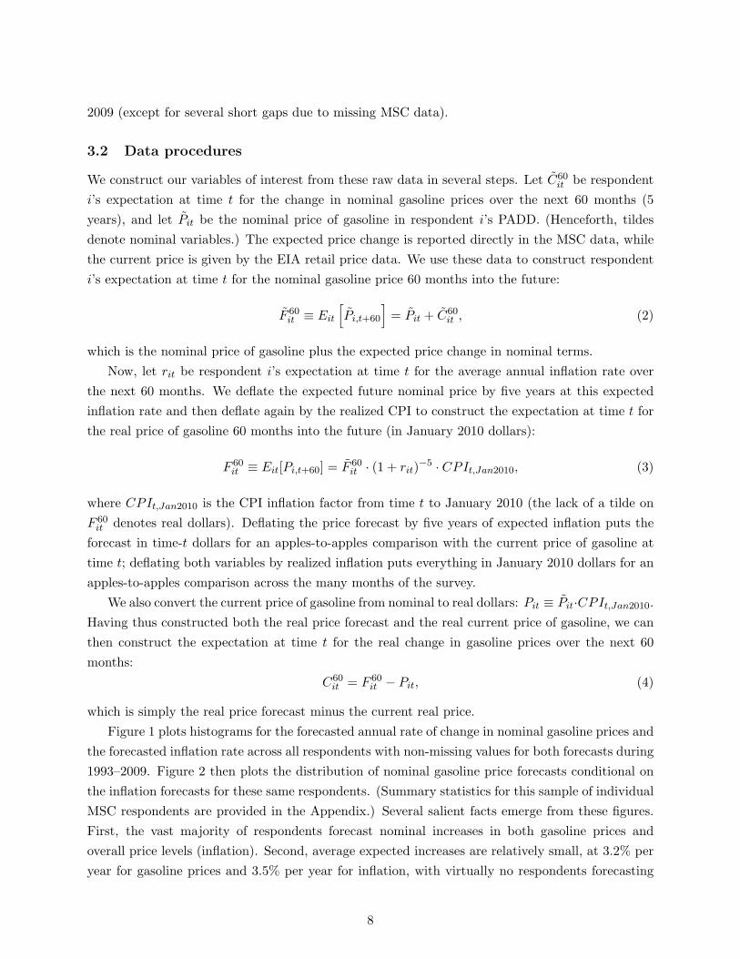
which is simply the real price forecast minus the current real price.Figure 1 plots histograms for the forecasted annual rate of change in nominal gasoline prices and

the forecasted inflation rate across all respondents with non-missing values for both forecasts during1993–2009. Figure 2 then plots the distribution of nominal gasoline price forecasts conditional onthe inflation forecasts for these same respondents. (Summary statistics for this sample of individualMSC respondents are provided in the Appendix.) Several salient facts emerge from these figures.First, the vast majority of respondents forecast nominal increases in both gasoline prices andoverall price levels (inflation). Second, average expected increases are relatively small, at 3.2% peryear for gasoline prices and 3.5% per year for inflation, with virtually no respondents forecasting

8

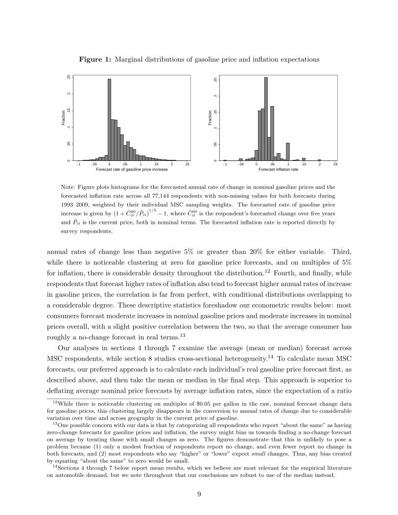
Figure 1: Marginal distributions of gasoline price and inflation expectations0

.05

.1.1

5.2

.25

Fra

ctio

n

-.1 -.05 0 .05 .1 .15 .2 .25

Forecast rate of gasoline price increase

0.0

5.1

.15

.2.2

5

Fra

ctio

n

-.1 -.05 0 .05 .1 .15 .2 .25

Forecast inflation rate

Note: Figure plots histograms for the forecasted annual rate of change in nominal gasoline prices and the

forecasted inflation rate across all 77,144 respondents with non-missing values for both forecasts during

1993–2009, weighted by their individual MSC sampling weights. The forecasted rate of gasoline price

increase is given by (1 + C60it /Pit)

1/5 − 1, where C60it is the respondent’s forecasted change over five years

and Pit is the current price, both in nominal terms. The forecasted inflation rate is reported directly by

survey respondents.

annual rates of change less than negative 5% or greater than 20% for either variable. Third,while there is noticeable clustering at zero for gasoline price forecasts, and on multiples of 5%for inflation, there is considerable density throughout the distribution.12 Fourth, and finally, whilerespondents that forecast higher rates of inflation also tend to forecast higher annual rates of increasein gasoline prices, the correlation is far from perfect, with conditional distributions overlapping toa considerable degree. These descriptive statistics foreshadow our econometric results below: mostconsumers forecast moderate increases in nominal gasoline prices and moderate increases in nominalprices overall, with a slight positive correlation between the two, so that the average consumer hasroughly a no-change forecast in real terms.13

Our analyses in sections 4 through 7 examine the average (mean or median) forecast acrossMSC respondents, while section 8 studies cross-sectional heterogeneity.14 To calculate mean MSCforecasts, our preferred approach is to calculate each individual’s real gasoline price forecast first, asdescribed above, and then take the mean or median in the final step. This approach is superior todeflating average nominal price forecasts by average inflation rates, since the expectation of a ratio

12While there is noticeable clustering on multiples of $0.05 per gallon in the raw, nominal forecast change datafor gasoline prices, this clustering largely disappears in the conversion to annual rates of change due to considerablevariation over time and across geography in the current price of gasoline.

13One possible concern with our data is that by categorizing all respondents who report “about the same” as havingzero-change forecasts for gasoline prices and inflation, the survey might bias us towards finding a no-change forecaston average by treating those with small changes as zero. The figures demonstrate that this is unlikely to pose aproblem because (1) only a modest fraction of respondents report no change, and even fewer report no change inboth forecasts, and (2) most respondents who say “higher” or “lower” expect small changes. Thus, any bias createdby equating “about the same” to zero would be small.

14Sections 4 through 7 below report mean results, which we believe are most relevant for the empirical literatureon automobile demand, but we note throughout that our conclusions are robust to use of the median instead.

9

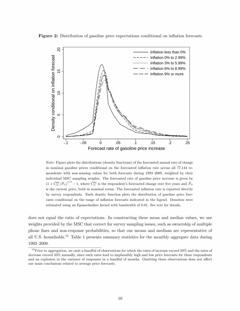
Figure 2: Distribution of gasoline price expectations conditional on inflation forecasts

05

1015

20

Den

sity

con

ditio

nal o

n in

flatio

n fo

reca

st

-.1 -.05 0 .05 .1 .15 .2 .25

Forecast rate of gasoline price increase

Inflation less than 0%

Inflation 0% to 2.99%



Inflation 9% or more

Note: Figure plots the distributions (density functions) of the forecasted annual rate of change

in nominal gasoline prices conditional on the forecasted inflation rate across all 77,144 re-

spondents with non-missing values for both forecasts during 1993–2009, weighted by their

individual MSC sampling weights. The forecasted rate of gasoline price increase is given by

(1 + C60it /Pit)

1/5 − 1, where C60it is the respondent’s forecasted change over five years and Pit

is the current price, both in nominal terms. The forecasted inflation rate is reported directly

by survey respondents. Each density function plots the distribution of gasoline price fore-

casts conditional on the range of inflation forecasts indicated in the legend. Densities were

estimated using an Epanechnikov kernel with bandwidth of 0.01. See text for details.

does not equal the ratio of expectations. In constructing these mean and median values, we useweights provided by the MSC that correct for survey sampling issues, such as ownership of multiplephone lines and non-response probabilities, so that our means and medians are representative ofall U.S. households.15 Table 1 presents summary statistics for the monthly aggregate data during1993–2009.

15Prior to aggregation, we omit a handful of observations for which the rates of increase exceed 50% and the rates ofdecrease exceed 33% annually, since such rates lead to implausibly high and low price forecasts for these respondentsand an explosion in the variance of responses in a handful of months. Omitting these observations does not affectour main conclusions related to average price forecasts.

10

Table 1: Summary statistics for monthly aggregate data

Variable Mean Std. Dev. Minimum Maximum

Real, levelsForecast gas price 2.089 0.722 1.272 4.544Current gas price 2.044 0.643 1.230 4.197Forecast gas price change 0.046 0.154 -0.143 0.816Real, logsForecast gas price 0.653 0.311 0.208 1.469Current gas price 0.671 0.282 0.204 1.434Forecast gas price change -0.018 0.064 -0.125 0.308Nominal, levelsForecast gas price 2.135 0.964 1.173 5.367Current gas price 1.765 0.736 0.971 4.112Forecast gas price change 0.370 0.257 0.106 1.260Nominal, logsForecast gas price 0.645 0.403 0.132 1.643Current gas price 0.492 0.376 -0.032 1.413Forecast gas price change 0.153 0.055 0.061 0.427

Note: Table reports summary statistics for sample of monthly aggregate data. Sample size is

189 months. See text for details.

4 Graphical analysis of mean consumer forecasts

We depict our price series graphically in figures 3 and 4. Figure 3 presents, in nominal terms, themean current price of gasoline (Pt), the mean forecast change over 5 years (C60

t ), and the meanforecast level (Ft) during our study period. The mean nominal expected change always exceedszero and rises with the increase in nominal gasoline prices over this time period. There is generallylittle month-to-month volatility in the mean forecast change, except in 2008, when gasoline pricesshot up and then plummeted during the financial crisis. This figure suggests that we would rejecta null hypothesis of a nominal no-change forecast: consumers consistently expect nominal gasolineprices to rise, and the expected change increases with the current nominal price.

The picture changes considerably after deflating by forecasted inflation. Figure 4 presents, inreal dollars, the mean price of gasoline (Pt), the mean forecast level (F 60

t ), and the mean forecastchange over 5 years (C60

t ). Note that the real forecast change hovers near zero for most of the studyperiod, with large deviations only around September 11, 2001 and the large price swings during thefinancial crisis of 2008. This figure suggests that the mean MSC respondent forecasts the real priceof gasoline in 5 years to equal the price at the time of the survey. That is, consumer forecasts areconsistent with a real no-change forecast. Intuitively, the two characteristics of the nominal datathat would lead to a rejection of a no-change forecast—the consistently positive forecast changeand the correlation between the expected change and current prices in levels—are both eliminatedwhen we account for expected inflation. Inflation alone will cause prices to rise over a five-yearhorizon, and a constant rate of inflation will have a larger impact on nominal prices in cents pergallon when the current price is higher.16

16Both figures 3 and 4 present prices in levels. The appendix includes figures in logged prices, where we first log

11

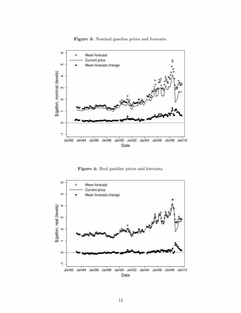
Figure 3: Nominal gasoline prices and forecasts.

−1

01

23

45

6

$/g

allo

n,

no

min

al (le

ve

ls)

Jan92 Jan94 Jan96 Jan98 Jan00 Jan02 Jan04 Jan06 Jan08 Jan10

Date

Mean forecast

Current price

Mean forecast change

Figure 4: Real gasoline prices and forecasts.

−1

01

23

45

6

$/g

allo

n,

rea

l (le

ve

ls)


Date

Mean forecast

Current price


12

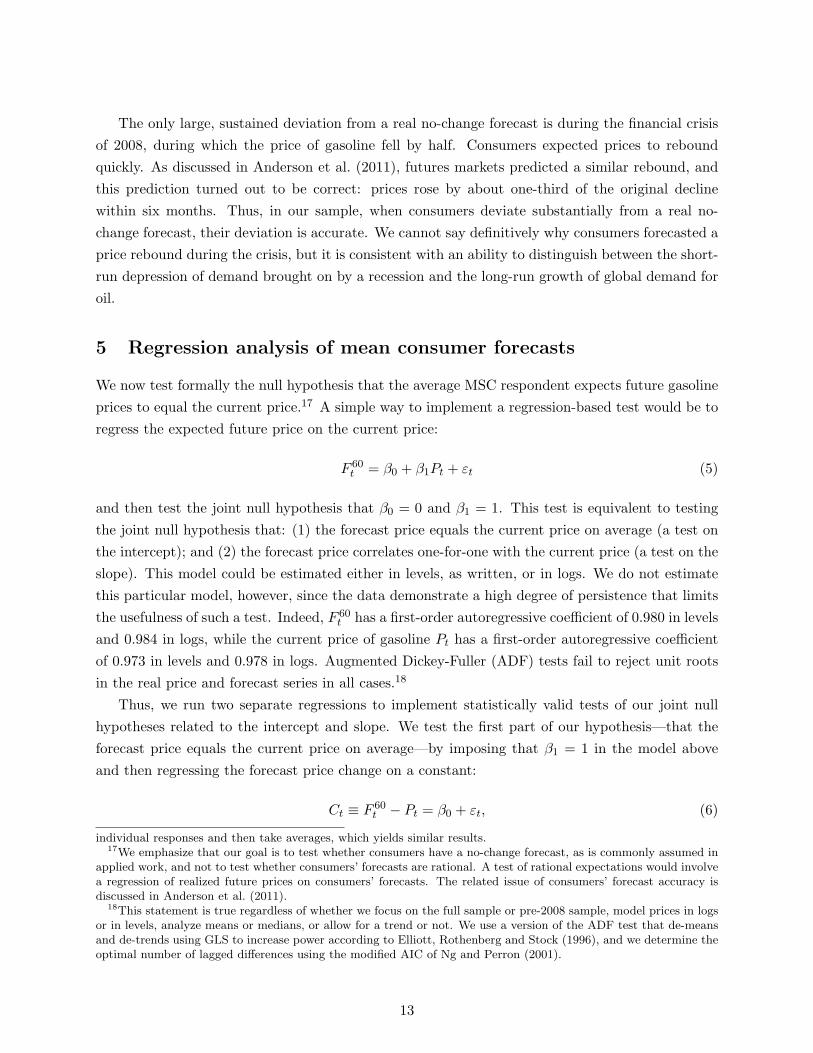
The only large, sustained deviation from a real no-change forecast is during the financial crisisof 2008, during which the price of gasoline fell by half. Consumers expected prices to reboundquickly. As discussed in Anderson et al. (2011), futures markets predicted a similar rebound, andthis prediction turned out to be correct: prices rose by about one-third of the original declinewithin six months. Thus, in our sample, when consumers deviate substantially from a real no-change forecast, their deviation is accurate. We cannot say definitively why consumers forecasted aprice rebound during the crisis, but it is consistent with an ability to distinguish between the short-run depression of demand brought on by a recession and the long-run growth of global demand foroil.

5 Regression analysis of mean consumer forecasts

We now test formally the null hypothesis that the average MSC respondent expects future gasolineprices to equal the current price.17 A simple way to implement a regression-based test would be toregress the expected future price on the current price:

F 60t = β0 + β1Pt + εt (5)

and then test the joint null hypothesis that β0 = 0 and β1 = 1. This test is equivalent to testingthe joint null hypothesis that: (1) the forecast price equals the current price on average (a test onthe intercept); and (2) the forecast price correlates one-for-one with the current price (a test on theslope). This model could be estimated either in levels, as written, or in logs. We do not estimatethis particular model, however, since the data demonstrate a high degree of persistence that limitsthe usefulness of such a test. Indeed, F 60

t has a first-order autoregressive coefficient of 0.980 in levelsand 0.984 in logs, while the current price of gasoline Pt has a first-order autoregressive coefficientof 0.973 in levels and 0.978 in logs. Augmented Dickey-Fuller (ADF) tests fail to reject unit rootsin the real price and forecast series in all cases.18

Thus, we run two separate regressions to implement statistically valid tests of our joint nullhypotheses related to the intercept and slope. We test the first part of our hypothesis—that theforecast price equals the current price on average—by imposing that β1 = 1 in the model aboveand then regressing the forecast price change on a constant:

Ct ≡ F 60t − Pt = β0 + εt, (6)

individual responses and then take averages, which yields similar results.17We emphasize that our goal is to test whether consumers have a no-change forecast, as is commonly assumed in

applied work, and not to test whether consumers’ forecasts are rational. A test of rational expectations would involvea regression of realized future prices on consumers’ forecasts. The related issue of consumers’ forecast accuracy isdiscussed in Anderson et al. (2011).

18This statement is true regardless of whether we focus on the full sample or pre-2008 sample, model prices in logsor in levels, analyze means or medians, or allow for a trend or not. We use a version of the ADF test that de-meansand de-trends using GLS to increase power according to Elliott, Rothenberg and Stock (1996), and we determine theoptimal number of lagged differences using the modified AIC of Ng and Perron (2001).

13

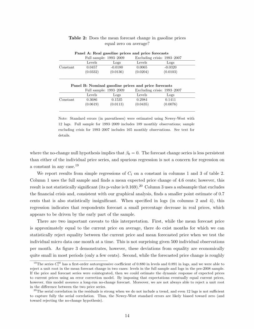
Table 2: Does the mean forecast change in gasoline pricesequal zero on average?

Panel A: Real gasoline prices and price forecastsFull sample: 1993–2009 Excluding crisis: 1993–2007

Levels Logs Levels Logs

Constant 0.0457 -0.0180 0.0065 -0.0320(0.0332) (0.0136) (0.0204) (0.0103)

Panel B: Nominal gasoline prices and price forecastsFull sample: 1993–2009 Excluding crisis: 1993–2007

Levels Logs Levels Logs

Constant 0.3686 0.1535 0.2984 0.1411(0.0619) (0.0113) (0.0435) (0.0076)

Note: Standard errors (in parentheses) were estimated using Newey-West with

12 lags. Full sample for 1993–2009 includes 189 monthly observations; sample

excluding crisis for 1993–2007 includes 165 monthly observations. See text for

details.

where the no-change null hypothesis implies that β0 = 0. The forecast change series is less persistentthan either of the individual price series, and spurious regression is not a concern for regression ona constant in any case.19

We report results from simple regressions of Ct on a constant in columns 1 and 3 of table 2.Column 1 uses the full sample and finds a mean expected price change of 4.6 cents; however, thisresult is not statistically significant (its p-value is 0.169).20 Column 3 uses a subsample that excludesthe financial crisis and, consistent with our graphical analysis, finds a smaller point estimate of 0.7cents that is also statistically insignificant. When specified in logs (in columns 2 and 4), thisregression indicates that respondents forecast a small percentage decrease in real prices, whichappears to be driven by the early part of the sample.

There are two important caveats to this interpretation. First, while the mean forecast priceis approximately equal to the current price on average, there do exist months for which we canstatistically reject equality between the current price and mean forecasted price when we test theindividual micro data one month at a time. This is not surprising given 500 individual observationsper month. As figure 3 demonstrates, however, these deviations from equality are economicallyquite small in most periods (only a few cents). Second, while the forecasted price change is roughly

19The series C60t has a first-order autoregressive coefficient of 0.880 in levels and 0.891 in logs, and we were able to

reject a unit root in the mean forecast change in two cases: levels in the full sample and logs in the pre-2008 sample.If the price and forecast series were cointegrated, then we could estimate the dynamic response of expected pricesto current prices using an error correction model. By imposing that expectations eventually equal current prices,however, this model assumes a long-run no-change forecast. Moreover, we are not always able to reject a unit rootin the difference between the two price series.

20The serial correlation in the residuals is strong when we do not include a trend, and even 12 lags is not sufficientto capture fully the serial correlation. Thus, the Newey-West standard errors are likely biased toward zero (andtoward rejecting the no-change hypothesis).

14

zero on average over the sample, there does appear to be a slight upward trend, with the earlierperiods (forecast price decline) balancing the later periods (forecast price increase). While thistrend might be consistent with growing concern about dwindling supplies of low-cost crude oil, thetrend is weak and the deviations from equality are small.

We test the second part of our hypothesis—that the forecast price varies one-for-one with thecurrent price—using the first-differenced equation 7, since both the forecasted and current priceseries are stationary in differences:

∆F 60t = β0 + β1∆Pt + εt. (7)

This first-differenced model is especially relevant for studies of automobile demand that rely ontime-series variation in gasoline prices to identify consumers’ valuation of fuel economy. Identifica-tion in such studies comes from observing how vehicle prices and quantities change in response tochanges in gasoline prices (typically interacted with vehicle efficiency). Thus, it is the response ofconsumers’ gasoline price forecasts to changes in the current price of gasoline that is most relevantin this and other literatures that rely on such identification.

Table 3 presents our regression results. Panel A presents results with real variables. Resultsin levels based on the full 1993–2009 sample imply that when the mean current price of gasolineincreases by $1.00, the mean real-price forecast increases by about $0.87. Results in logs basedon the full sample imply that when the current price of gasoline increases by 1%, the mean real-price forecast increases by about 0.83%. We cannot statistically reject the null hypothesis of areal no-change forecast at a conventional 5% level, but this is partly because estimates using thefull sample have sizable standard errors. The point estimates are economically significant. Theysuggest less-than-full adjustment, so that consumers anticipate mean-reverting gasoline prices.

This result (and much of the imprecision) is driven by the data from the financial crisis of 2008,which led to a large deviation between the current and expected future price. When we limit thesample to the 1993–2007 period, as reported in the right-hand side of the table, the regressioncoefficients are all tightly estimated and close to 1, consistent with a no-change forecast. Resultsin levels based on the limited 1993–2007 sample imply that when the current price of gasolineincreases by $1.00, the mean forecast price increases by $0.99. The estimates reject even modestdeviations from the no-change null hypothesis with a narrow 95% confidence interval of $0.91 to$1.07. Results in logs based on the limited sample imply that when the current price increases by1%, the mean forecast price increases by 0.96%. Again, the estimates reject even modest deviationsfrom the no-change null with a 95% confidence interval of 0.89% to 1.07%.

Figure 5 presents these results graphically: forecasted gasoline prices increase one-for-one withcurrent prices on average. To highlight the importance of the financial crisis, data from 2008 and2009 are denoted with x’s. These observations clearly have the largest residuals. This figure alsoillustrates that while the slope is one, the correlation is not perfect, even during normal times.Thus, the current price is a somewhat noisy measure of average stated beliefs.

In table 3 panel B, we do not adjust for inflation, but rather regress changes in the mean

15

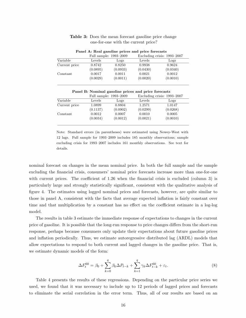
Table 3: Does the mean forecast gasoline price changeone-for-one with the current price?


Variable Levels Logs Levels Logs

Current price 0.8742 0.8250 0.9938 0.9624(0.0895) (0.0933) (0.0430) (0.0340)

Constant 0.0017 0.0011 0.0021 0.0012(0.0029) (0.0011) (0.0020) (0.0010)



Current price 1.0899 0.8804 1.2571 1.0147(0.1137) (0.0902) (0.0299) (0.0268)

Constant 0.0012 0.0007 0.0010 0.0005(0.0034) (0.0012) (0.0021) (0.0010)

Note: Standard errors (in parentheses) were estimated using Newey-West with


excluding crisis for 1993–2007 includes 161 monthly observations. See text for

details.

nominal forecast on changes in the mean nominal price. In both the full sample and the sampleexcluding the financial crisis, consumers’ nominal price forecasts increase more than one-for-onewith current prices. The coefficient of 1.26 when the financial crisis is excluded (column 3) isparticularly large and strongly statistically significant, consistent with the qualitative analysis offigure 4. The estimates using logged nominal prices and forecasts, however, are quite similar tothose in panel A, consistent with the facts that average expected inflation is fairly constant overtime and that multiplication by a constant has no effect on the coefficient estimate in a log-logmodel.

The results in table 3 estimate the immediate response of expectations to changes in the currentprice of gasoline. It is possible that the long-run response to price changes differs from the short-runresponse, perhaps because consumers only update their expectations about future gasoline pricesand inflation periodically. Thus, we estimate autoregressive distributed lag (ARDL) models thatallow expectations to respond to both current and lagged changes in the gasoline price. That is,we estimate dynamic models of the form:

∆F 60t = β0 +

q∑k=0

βk∆Pt−k +q∑

k=1

γk∆F 60t−k + εt. (8)

Table 4 presents the results of these regressions. Depending on the particular price series weused, we found that it was necessary to include up to 12 periods of lagged prices and forecaststo eliminate the serial correlation in the error term. Thus, all of our results are based on an

16

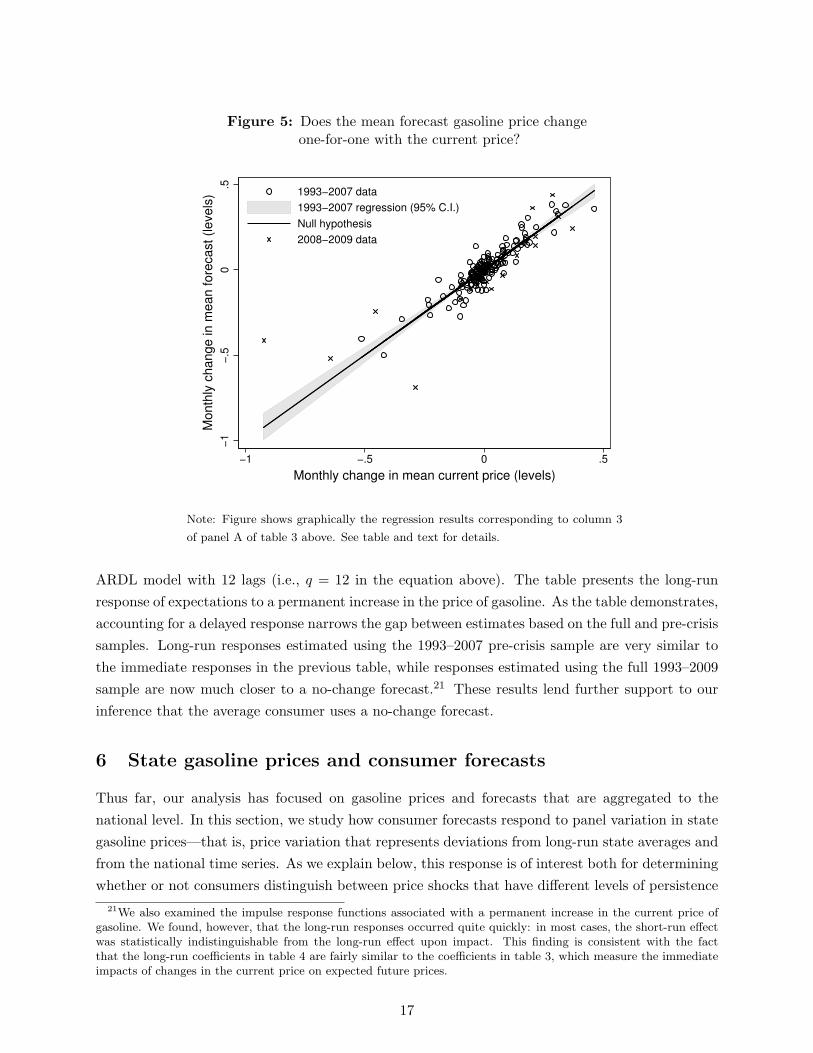
Figure 5: Does the mean forecast gasoline price changeone-for-one with the current price?

−1

−.5

0.5

Month

ly c

hange in m

ean fore

cast (levels

)

−1 −.5 0 .5

Monthly change in mean current price (levels)

1993−2007 data

1993−2007 regression (95% C.I.)

Null hypothesis

2008−2009 data

Note: Figure shows graphically the regression results corresponding to column 3

of panel A of table 3 above. See table and text for details.

ARDL model with 12 lags (i.e., q = 12 in the equation above). The table presents the long-runresponse of expectations to a permanent increase in the price of gasoline. As the table demonstrates,accounting for a delayed response narrows the gap between estimates based on the full and pre-crisissamples. Long-run responses estimated using the 1993–2007 pre-crisis sample are very similar tothe immediate responses in the previous table, while responses estimated using the full 1993–2009sample are now much closer to a no-change forecast.21 These results lend further support to ourinference that the average consumer uses a no-change forecast.

6 State gasoline prices and consumer forecasts

Thus far, our analysis has focused on gasoline prices and forecasts that are aggregated to thenational level. In this section, we study how consumer forecasts respond to panel variation in stategasoline prices—that is, price variation that represents deviations from long-run state averages andfrom the national time series. As we explain below, this response is of interest both for determiningwhether or not consumers distinguish between price shocks that have different levels of persistence

21We also examined the impulse response functions associated with a permanent increase in the current price ofgasoline. We found, however, that the long-run responses occurred quite quickly: in most cases, the short-run effectwas statistically indistinguishable from the long-run effect upon impact. This finding is consistent with the factthat the long-run coefficients in table 4 are fairly similar to the coefficients in table 3, which measure the immediateimpacts of changes in the current price on expected future prices.

17

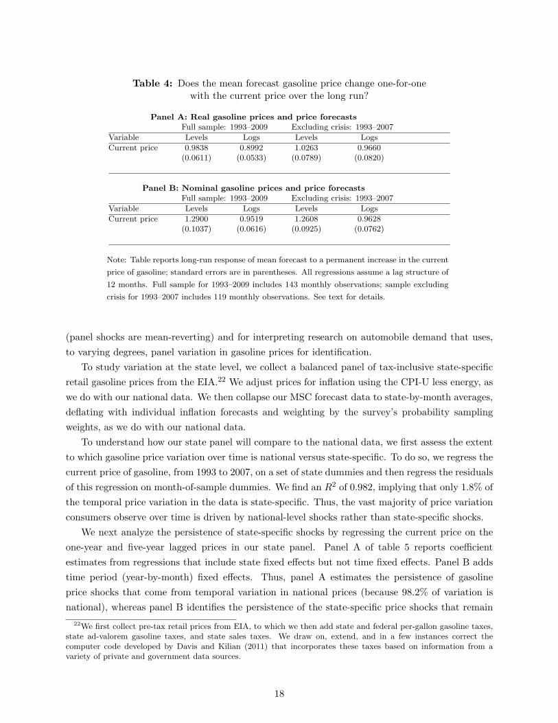
Table 4: Does the mean forecast gasoline price change one-for-onewith the current price over the long run?



Current price 0.9838 0.8992 1.0263 0.9660(0.0611) (0.0533) (0.0789) (0.0820)



Current price 1.2900 0.9519 1.2608 0.9628(0.1037) (0.0616) (0.0925) (0.0762)

Note: Table reports long-run response of mean forecast to a permanent increase in the current

price of gasoline; standard errors are in parentheses. All regressions assume a lag structure of

12 months. Full sample for 1993–2009 includes 143 monthly observations; sample excluding

crisis for 1993–2007 includes 119 monthly observations. See text for details.

(panel shocks are mean-reverting) and for interpreting research on automobile demand that uses,to varying degrees, panel variation in gasoline prices for identification.

To study variation at the state level, we collect a balanced panel of tax-inclusive state-specificretail gasoline prices from the EIA.22 We adjust prices for inflation using the CPI-U less energy, aswe do with our national data. We then collapse our MSC forecast data to state-by-month averages,deflating with individual inflation forecasts and weighting by the survey’s probability samplingweights, as we do with our national data.

To understand how our state panel will compare to the national data, we first assess the extentto which gasoline price variation over time is national versus state-specific. To do so, we regress thecurrent price of gasoline, from 1993 to 2007, on a set of state dummies and then regress the residualsof this regression on month-of-sample dummies. We find an R2 of 0.982, implying that only 1.8% ofthe temporal price variation in the data is state-specific. Thus, the vast majority of price variationconsumers observe over time is driven by national-level shocks rather than state-specific shocks.

We next analyze the persistence of state-specific shocks by regressing the current price on theone-year and five-year lagged prices in our state panel. Panel A of table 5 reports coefficientestimates from regressions that include state fixed effects but not time fixed effects. Panel B addstime period (year-by-month) fixed effects. Thus, panel A estimates the persistence of gasolineprice shocks that come from temporal variation in national prices (because 98.2% of variation isnational), whereas panel B identifies the persistence of the state-specific price shocks that remain

22We first collect pre-tax retail prices from EIA, to which we then add state and federal per-gallon gasoline taxes,state ad-valorem gasoline taxes, and state sales taxes. We draw on, extend, and in a few instances correct thecomputer code developed by Davis and Kilian (2011) that incorporates these taxes based on information from avariety of private and government data sources.

18

Table 5: How persistent are state-specific gasoline price shocks?

Panel A: Real gasoline price autoregressions with state fixed effectsTwelve-month lags Sixty-month lags


Lagged price 0.9992 1.0256 0.4877 1.7327(0.0636) (0.0398) (0.2213) (0.1482)

Panel B: Real gasoline price autoregressionswith time and state fixed effects

Twelve-month lags Sixty-month lags


Lagged price 0.2565 0.3199 0.1280 0.1132(0.0570) (0.0607) (0.0489) (0.0440)

Dependent variable is the current real price of gasoline in a month and state. The

lagged price is a 12-month lag in columns 1 and 2 and a 60-month lag in columns

3 and 4. Variables are not first differenced. Standard errors (in parentheses) are

two-way clustered on state and month-of-sample. Panel A includes state fixed

effects. Panel B includes state and month fixed effects. Sample is pre-crisis, from

1993–2007, with 9,000 observations for columns 1 and 2 and 7,200 observations

for columns 3 and 4.

after removing the national time series.Table 5 shows that national shocks are far more persistent than state-specific shocks. The one-

year lagged coefficients in panel A are very close to 1. In contrast, the corresponding estimates inpanel B show that, on average, only one-quarter to one-third of an idiosyncratic price shock in astate today will persist one year later. The five-year lagged coefficients tell a qualitatively similarstory, though these estimates are sensitive to the exact specification used and are impreciselyestimated in the absence of month-of-sample fixed effects.23 These estimates accord with intuition:idiosyncratic state-level shocks, such as local refinery outages, are typically short-lived and can beeliminated by market forces. National-level price variation, however, is primarily driven by crudeoil prices that are set globally and well-approximated by a random walk.

We next turn to our consumer forecast data and ask whether or not consumers react differentlyto national and state price shocks when forming their forecasts. A fully informed and rationalconsumer would predict significant mean reversion for state-specific gasoline price shocks, but itmay be difficult for consumers to distinguish between price movements that are national and thosethat are specific to their states. Table 6 reports estimates from regressions of the forecasted priceon the current price (in first differences), mimicking our main specification from table 3, using thestate panel. We vary the inclusion of time fixed effects to show how consumer forecasts change

23Further, the five-year coefficients vary when logs are used instead of levels, when we change the exact time periodused, and when we weight by the number of MSC respondents so as to better mimic the identification in our forecastregressions. Nevertheless, across all specifications we have analyzed we find that state-specific deviations exhibit farless persistence than national time series changes.

19

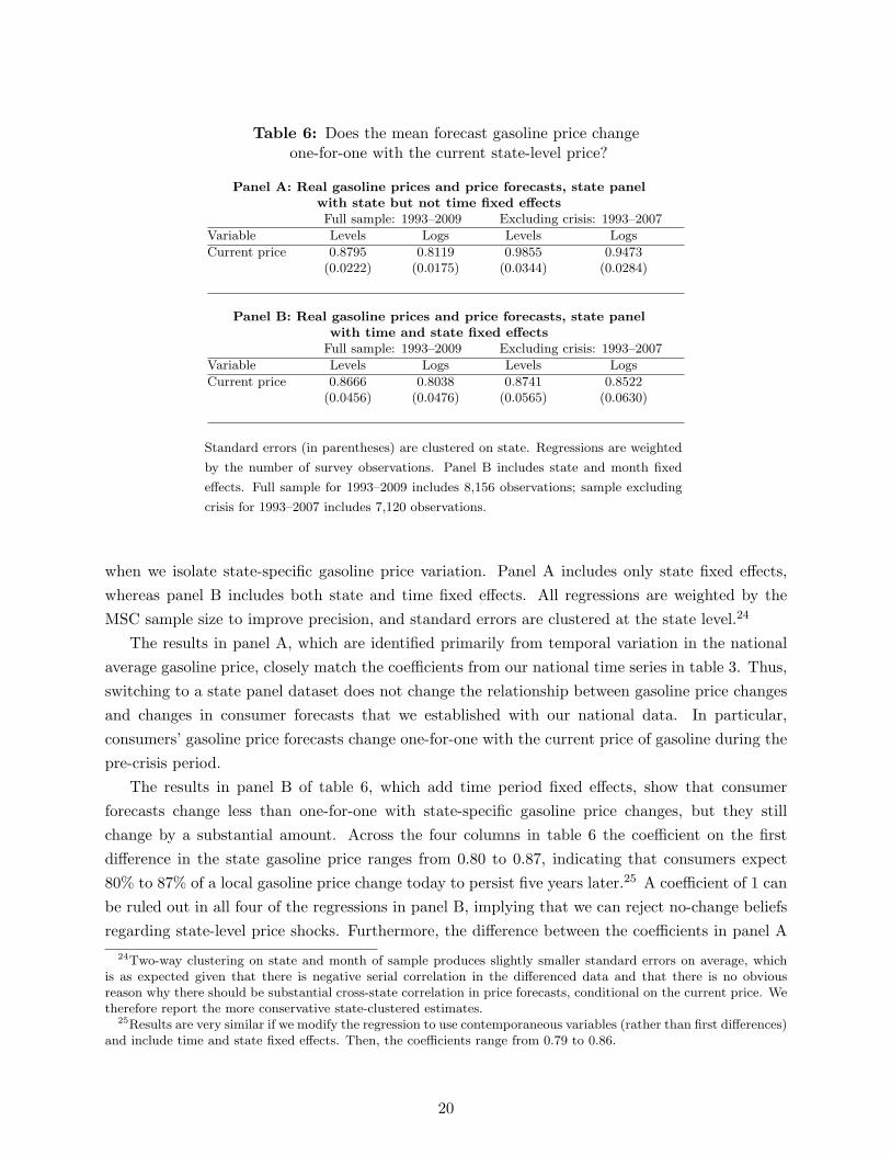
Table 6: Does the mean forecast gasoline price changeone-for-one with the current state-level price?

Panel A: Real gasoline prices and price forecasts, state panelwith state but not time fixed effectsFull sample: 1993–2009 Excluding crisis: 1993–2007


Current price 0.8795 0.8119 0.9855 0.9473(0.0222) (0.0175) (0.0344) (0.0284)

Panel B: Real gasoline prices and price forecasts, state panelwith time and state fixed effects

Full sample: 1993–2009 Excluding crisis: 1993–2007


Current price 0.8666 0.8038 0.8741 0.8522(0.0456) (0.0476) (0.0565) (0.0630)

Standard errors (in parentheses) are clustered on state. Regressions are weighted

by the number of survey observations. Panel B includes state and month fixed

effects. Full sample for 1993–2009 includes 8,156 observations; sample excluding

crisis for 1993–2007 includes 7,120 observations.

when we isolate state-specific gasoline price variation. Panel A includes only state fixed effects,whereas panel B includes both state and time fixed effects. All regressions are weighted by theMSC sample size to improve precision, and standard errors are clustered at the state level.24

The results in panel A, which are identified primarily from temporal variation in the nationalaverage gasoline price, closely match the coefficients from our national time series in table 3. Thus,switching to a state panel dataset does not change the relationship between gasoline price changesand changes in consumer forecasts that we established with our national data. In particular,consumers’ gasoline price forecasts change one-for-one with the current price of gasoline during thepre-crisis period.

The results in panel B of table 6, which add time period fixed effects, show that consumerforecasts change less than one-for-one with state-specific gasoline price changes, but they stillchange by a substantial amount. Across the four columns in table 6 the coefficient on the firstdifference in the state gasoline price ranges from 0.80 to 0.87, indicating that consumers expect80% to 87% of a local gasoline price change today to persist five years later.25 A coefficient of 1 canbe ruled out in all four of the regressions in panel B, implying that we can reject no-change beliefsregarding state-level price shocks. Furthermore, the difference between the coefficients in panel A

24Two-way clustering on state and month of sample produces slightly smaller standard errors on average, whichis as expected given that there is negative serial correlation in the differenced data and that there is no obviousreason why there should be substantial cross-state correlation in price forecasts, conditional on the current price. Wetherefore report the more conservative state-clustered estimates.

25Results are very similar if we modify the regression to use contemporaneous variables (rather than first differences)and include time and state fixed effects. Then, the coefficients range from 0.79 to 0.86.

20

and panel B is statistically significant for the pre-crisis sample but not for the full sample.26

Thus, when we identify our coefficient using only state-specific gasoline price changes, consumerforecasts do display some mean reversion. Nevertheless, this level of mean reversion is far below theactual mean reversion we estimate in table 5. We interpret this result as evidence that consumerscannot readily distinguish between price fluctuations that occur locally and those that reflect ag-gregate factors. Local gasoline prices are salient to consumers, but under normal circumstancesmost consumers will have little information on gasoline prices in other states. It is therefore notobvious how consumers would distinguish idiosyncratic state-specific variation from national varia-tion, particularly given that national-level factors are by far the dominant driver of price changes.As a result, consumers treat all gasoline price changes as being highly persistent.

Our findings carry implications for research that uses a panel research design to study consumerdecisions that require forecasting. For example, Busse et al. (Forthcoming) runs regressions ofvehicle prices and market shares on local gasoline prices to gain insight into how consumers’ demandfor fuel economy responds to gasoline prices. To the extent that controls for national-level pricesare included in the regressions (the paper varies its use of these controls across robustness checks),the results will be driven more by state-level variation and less by national variation.27 Ex-ante,our “rational consumer” priors suggest that papers such as Busse et al. (Forthcoming) should beleery of relying solely or even partially on state-level idiosyncratic variation to identify parametersrelated to durable investment decisions—particularly when these parameters are subsequently usedto simulate impacts of permanent gasoline price or tax changes—as this variation is transitory andmean-reverting.

Fully-informed, rational consumers should largely ignore state-specific price shocks when pur-chasing new vehicles. However, our results in table 6 suggest that consumers actually perceivestate-level price variation to be quite persistent, suggesting that approaches relying on state-levelvariation may nonetheless yield valid estimates. Overall, our panel analysis should serve as a re-minder to researchers that the relationship between consumer forecasts and current prices maydepend on what price variation is used for identification. Researchers should be cautious when us-ing local gasoline price variation and not take for granted that expected future prices equal current

26To test the difference between the panel A and B results, we cluster bootstrap our data on state and estimatethe coefficient including and excluding time fixed effects for each drawn sample. We then compare the distributionof estimated coefficients across trials. The coefficient distributions with and without the fixed effects are very similarfor the full sample, but our bootstrap test of the difference in coefficients for the pre-crisis sample produces p-valuesof 0.052 and 0.057 for the level and log specifications respectively.

27The main specifications of Busse et al. (Forthcoming) use year fixed effects, though the fact that the data aremonthly implies that most of the gasoline price variation used (82% of it, per our calculations) is still at the nationallevel. In a robustness test of the paper’s new vehicle quantity results, month-of-sample fixed effects are used. Thistest yields similar estimates to what was found in the main specification, though with much larger standard errors.This outcome reflects our findings that: (1) consumers forecast state-level shocks as being highly persistent; and (2)state-level variation is quite small relative to national-level variation. The paper’s vehicle price regressions also usemonth-of-sample fixed effects in a robustness test. However, in this case, the critical coefficient is for the interactionof the gasoline price with fuel economy, so that identification is still largely coming from national-level gasoline pricevariation. Other papers in this literature that include time-period fixed effects, such as Allcott and Wozny (2011)and Li et al. (2009), also focus on interactions between fuel economy and gasoline prices, thereby avoiding a strongreliance on state-level variation.

21

prices in all specifications.

7 Do forecasts respond differently to tax and pre-tax price changes?

Our analysis of the state panel also allows us to comment on a literature that examines whetheror not consumers respond differently to the tax and non-tax components of gasoline prices. Muchof the research examining the effects of gasoline prices is motivated by policy questions about theefficacy of corrective taxation to reduce gasoline-related externalities. This research typically usesgasoline price variation driven primarily by global oil price fluctuations that pass through into retailprices, and then uses derived elasticities to predict how a tax change would influence consumption.

Davis and Kilian (2011) and Li et al. (2012), however, argue that gasoline consumption respondsmuch more strongly to changes in gasoline taxes than it does to pre-tax gasoline price changes.This argument implies that prior research has underestimated the effectiveness of gasoline taxesat reducing externalities. For example, Davis and Kilian (2011) uses taxes as instruments for thetax-inclusive price in a state panel dataset and estimates that a 10-cent gasoline tax could lowercarbon emissions from vehicles in the U.S. by 1.5%. This estimate is two-and-a-half times largerthan the effect implied by the paper’s OLS estimates.

Both Davis and Kilian (2011) and Li et al. (2012) use a state panel to run regressions ofcurrent gasoline consumption on current gasoline prices and rely fully on state-level variation toidentify the consumption elasticity. Their challenge is then to explain why consumers would responddifferently to the two components of price, given that posted prices in this market are always tax-inclusive. Both papers emphasize that taxes and non-tax price changes may have different impactson consumer expectations of future prices. Consumers may expect gasoline price changes that aredue to tax policy to be more persistent than those due to fluctuations in supply and demand. As aresult, tax changes may be more likely to lead consumers to make long-run investments that lowergasoline consumption.

The model implicit in this reasoning is that current consumption is a function both of thecurrent price of gasoline and consumer expectations about the future price. We specify this modelhere in an additive linear form:

ln(Cst) = β ln(Pst + τst) + γ ln(F kst(Pst, τst)) + αs + δt, (9)

where the subscript t denotes the current period, s denotes state, and the superscript k denotessome future period. C is current gasoline consumption; F is a forecast of future gasoline prices,which is a function of both current taxes τ and current pre-tax prices P ; α are state fixed effects;and δ are time period fixed effects.

Taking derivatives of equation 9 and rearranging, we can write the difference between themarginal effect of a tax change (in cents per gallon) on logged gasoline consumption and the

22

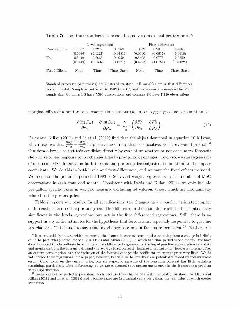
Table 7: Does the mean forecast respond equally to taxes and pre-tax prices?

Level regressions First differences

Pre-tax price 1.1037 1.2279 0.8769 1.0042 0.9075 0.9081(0.0086) (0.1227) (0.0451) (0.0330) (0.0617) (0.0618)

Tax 0.5449 0.7666 0.4950 0.5408 0.0775 0.0859(0.1449) (0.1397) (0.1771) (0.4793) (1.0781) (1.10828)

Fixed Effects None Time Time, State None Time Time, State

Standard errors (in parentheses) are clustered on state. All variables are in first differences

in columns 4-6. Sample is restricted to 1993 to 2007, and regressions are weighted by MSC

sample size. Columns 1-3 have 7,593 observations and columns 4-6 have 7,120 observations.

marginal effect of a pre-tax price change (in cents per gallon) on logged gasoline consumption as:

∂ ln(Cst)∂τst

− ∂ ln(Cst)∂Pst

=γ

F kst·(∂F kst∂τst

− ∂F kst∂Pst

). (10)

Davis and Kilian (2011) and Li et al. (2012) find that the object described in equation 10 is large,which requires that ∂Fk

st∂τst

− ∂Fkst

∂Pstbe positive, assuming that γ is positive, as theory would predict.28

Our data allow us to test this condition directly by evaluating whether or not consumers’ forecastsshow more or less response to tax changes than to pre-tax price changes. To do so, we run regressionsof our mean MSC forecast on both the tax and pre-tax price (adjusted for inflation) and comparecoefficients. We do this in both levels and first-differences, and we vary the fixed effects included.We focus on the pre-crisis period of 1993 to 2007 and weight regressions by the number of MSCobservations in each state and month. Consistent with Davis and Kilian (2011), we only includeper-gallon specific taxes in our tax measure, excluding ad-valorem taxes, which are mechanicallyrelated to the pre-tax price.

Table 7 reports our results. In all specifications, tax changes have a smaller estimated impacton forecasts than does the pre-tax price. The difference in the estimated coefficients is statisticallysignificant in the levels regressions but not in the first differenced regressions. Still, there is nosupport in any of the estimates for the hypothesis that forecasts are especially responsive to gasolinetax changes. This is not to say that tax changes are not in fact more persistent.29 Rather, our

28It seems unlikely that γ, which represents the change in current consumption resulting from a change in beliefs,could be particularly large, especially in Davis and Kilian (2011), in which the time period is one month. We havedirectly tested this hypothesis by running a first-differenced regression of the log of gasoline consumption in a stateand month on both the current price and the average MSC forecast. Estimates indicate that forecasts have no effecton current consumption, and the inclusion of the forecast changes the coefficient on current price very little. We donot include these regressions in the paper, however, because we believe they are potentially biased by measurementerror. Conditional on the current price, our state-specific measure of the consumer forecast has little variationremaining, particularly after differencing, so we are concerned that measurement error in the forecast is a problemin this specification.

29Taxes will not be perfectly persistent, both because they change relatively frequently (as shown by Davis andKilian (2011) and Li et al. (2012)) and because taxes are in nominal cents per gallon, the real value of which erodesover time.

23

regressions suggest that consumers do not readily distinguish between tax and non-tax changes inmaking forecasts. This result might not be surprising given that most tax changes are small (andtherefore may go unnoticed) and that taxes are never separately listed at the pump. It is alsoconsistent with our finding in section 6 that consumers do not distinguish between national andstate-specific price shocks. In sum, our forecast data do not provide support for the hypothesis,suggested by other researchers, that excess sensitivity of forecasts to tax changes is likely to explainthe finding that current gasoline consumption is more sensitive to tax policy than to pre-tax pricechanges.

8 Heterogeneity in consumer forecasts

Thus far, we have focused on mean consumer beliefs by studying the average of the MSC responseseach month. Here, we investigate the heterogeneity in consumers’ forecasts that is present in theindividual-level MSC data. These data demonstrate what we consider to be substantial forecastdispersion across respondents in each MSC survey month. In our sample, the average standarddeviation of the real five-year price forecast across respondents within a month is 62 cents (thecorresponding standard deviation of logged forecasts is 0.25).30 In what follows, we ask how thisheterogeneity relates to individual-level factors such as demographics, how it varies over time, andhow it compares to other sources of heterogeneity that affect consumers’ valuation of fuel economy.

Variation across individual survey responses could be interpreted in several ways. Dispersioncould reflect true disagreement across individuals. Alternatively, it could constitute a measure ofuncertainty, or it could simply reflect random noise in the survey instrument. In Anderson et al.(2011), we consider the possibility that dispersion reflects uncertainty, but we fail to find a strongcorrelation between the MSC dispersion and two measures of oil price volatility in the years priorto the financial crisis. And, while we cannot rule out that noise exists in our data, we show belowthat a large fraction of the dispersion persists across individuals who are surveyed twice. Thus,our preferred interpretation is the former, that dispersion reflects disagreement across individualsin their forecasts of the future price. This interpretation accords with prior literature (Mankiw,Reis and Wolfers 2004; Curtin 2010) and is consistent with the fact that the survey elicits a pointestimate from each individual.

Throughout this section, we discuss how we believe our findings inform research on consumerdemand for energy-consuming durable goods. This literature has for the most part assumed awayfactors that would lead to heterogeneity in valuation of energy efficiency. In the context of vehicledemand, these factors include not just heterogeneity in future price forecasts but also in vehiclemiles traveled, local gasoline prices, and consumers’ discount rates. Some recent papers, however,have begun to explore the econometric and policy implications of heterogeneity. Bento et al. (2012)studies the estimation of vehicle demand models like those in our equation (1), and finds that

30We obtain these figures by regressing the forecasts (for the entire sample period, not just the pre-crisis period)on month-of-sample dummies and then taking the standard deviation of the residuals. We continue to omit extremeoutliers as discussed in footnote 15 above.

24

assuming homogeneity can lead to biased estimates of the average consumer’s willingness to payfor fuel economy.31 Allcott et al. (2012) presents a model of optimal taxation in the presence ofconsumers that are myopic about future energy expenses and exhibit heterogeneity in the intensityof their use of energy-consuming durables (i.e., heterogeneity in miles traveled in the case of vehi-cles). The paper does not discuss, however, heterogeneity in consumers’ forecasts of future energyprices. It is our hope that the results below will provide useful guidance to this nascent literatureas it continues to explore the implications of consumer heterogeneity.

8.1 What explains forecast heterogeneity?

We begin by examining how much of the variation in consumers’ price forecasts is predictable, basedon observable characteristics of the respondents. Within the MSC dataset we observe demographicinformation such as age, income, and education that might plausibly be correlated with gasolineprice forecasts. To quantify these correlations in the data, we first strip out aggregate factorsby regressing the individual real forecasts on month-of-sample fixed effects. We then regress theresiduals from this regression on an income polynomial and on dummy variable categories foreducation, race, marital status, gender, and state of residence. This regression yields an R2 of only0.053 when run in levels and 0.078 when run in logs. Some demographic factors have a statisticallysignificant impact on forecasts, but these effects tend to be small in magnitude. For instance,males’ forecasts are on average 12 cents higher than females’ forecasts, and college graduates haveforecasts that are on average 5 cents higher than those of high school graduates with no collegeeducation. Overall, however, it appears that observable demographic factors explain very little ofthe forecast heterogeneity across respondents.

A related issue concerns the extent to which forecasts are stable for each individual. That is,is it the case that someone who has a relatively high forecast today will also have a relatively highforecast tomorrow? Because many of the MSC respondents appear in the sample twice, six monthsapart, we are able to address this question through regressions with individual fixed effects. Wefirst limit the sample to the 26,384 respondents for whom we have 2 observations. We then regressthese respondents’ real price forecasts on month-of-sample dummies and the local gasoline priceand then regress the residuals from this regression on a set of individual fixed effects. The R2 of thissecond regression is 0.65 in levels and 0.66 in logs, implying that the majority of the heterogeneityin the data is stable within individuals.

This result implies that, while there may be considerable heterogeneity in consumers’ futuregasoline price forecasts, changes in consumers’ forecasts over time (largely in response to currentgas price changes) exhibit substantially smaller cross-sectional variation. This finding is relevantfor investigations of consumers’ valuation of fuel economy because research in this area typicallyrelies on time series variation in gasoline prices for identification.32 To the extent that different

31The bias cannot be definitively signed, although the example provided in the paper suggests that it is towardzero.

32Estimation strategies that instead use only cross-sectional variation in vehicle market shares, characteristics, andprices are generally now viewed as plagued by omitted variables bias arising from unobservable vehicle characteristics

25

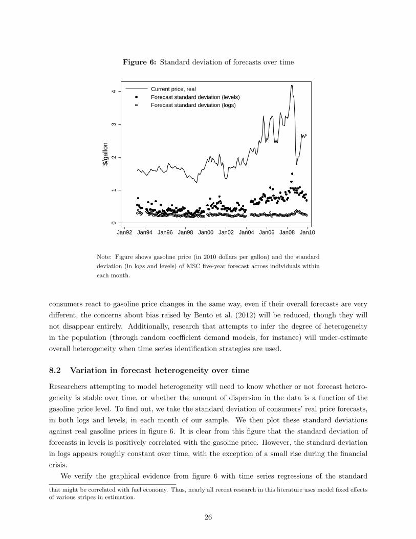
Figure 6: Standard deviation of forecasts over time

01

23

4

$/ga

llon


Current price, real

Forecast standard deviation (levels)Forecast standard deviation (logs)

Note: Figure shows gasoline price (in 2010 dollars per gallon) and the standard

deviation (in logs and levels) of MSC five-year forecast across individuals within

each month.

consumers react to gasoline price changes in the same way, even if their overall forecasts are verydifferent, the concerns about bias raised by Bento et al. (2012) will be reduced, though they willnot disappear entirely. Additionally, research that attempts to infer the degree of heterogeneityin the population (through random coefficient demand models, for instance) will under-estimateoverall heterogeneity when time series identification strategies are used.

8.2 Variation in forecast heterogeneity over time

Researchers attempting to model heterogeneity will need to know whether or not forecast hetero-geneity is stable over time, or whether the amount of dispersion in the data is a function of thegasoline price level. To find out, we take the standard deviation of consumers’ real price forecasts,in both logs and levels, in each month of our sample. We then plot these standard deviationsagainst real gasoline prices in figure 6. It is clear from this figure that the standard deviation offorecasts in levels is positively correlated with the gasoline price. However, the standard deviationin logs appears roughly constant over time, with the exception of a small rise during the financialcrisis.

We verify the graphical evidence from figure 6 with time series regressions of the standard

that might be correlated with fuel economy. Thus, nearly all recent research in this literature uses model fixed effectsof various stripes in estimation.

26

Table 8: Does the standard deviation of consumers’ forecasts vary with the gasoline price?

Full sample: 1993–2009 Excluding crisis: 1993–2007


Gasoline Price .216 -0.012 0.325 0.068(0.081) (0.053) (0.070) (0.038)

Dependent variable is the standard deviation of the MSC forecasts within each

month. Standard errors (in parentheses) were estimated using Newey-West with


excluding crisis for 1993–2007 includes 161 monthly observations.

deviation of the MSC forecast on the gasoline price. Results are reported in table 8, which confirmsa strong, positive statistical association between the gasoline price and variance of the forecasts inlevels but little relationship between these variables in logs.

We conclude from this analysis that researchers interested in modeling heterogeneity shouldbe wary of assuming a constant variance of gasoline price forecasts if modeled in levels, but thatdoing so in logs appears to be consistent with the data. Bento et al. (2012) show that ignoringheterogeneity can lead to biased estimates of the average consumer’s valuation of fuel economy; ourresults thus imply that temporal variation in heterogeneity can then lead to temporal variation inthe magnitude of this bias that is correlated with gasoline prices.

8.3 Comparison of forecast heterogeneity to other sources

Heterogeneity in consumer forecasts may be important for studies of fuel economy demand, butequation 1 above emphasizes that there are several such sources of heterogeneity. Differencesacross individuals in miles traveled, discounting, and local gasoline prices will also contribute toheterogeneity in consumer valuation of fuel economy. Is forecast heterogeneity important whencompared with these other factors?

We study this issue via a simulation in which we independently draw 100,000 values for annualmiles driven, discount rates, local gasoline prices, and gasoline price forecasts from their respectiveempirical (or calibrated parametric) distributions.33 For each draw, we calculate the present value

33To model heterogeneity in miles driven, we take independent draws from a lognormal distribution calibrated tomatch the mean and variance across households of annual vehicle miles per driver, as reported by Li et al. (2012),based on National Household Transportation Survey data from 1995 and 2001 for households that report two odometerreadings for each vehicle they own. The distribution of annual vehicle miles per household is highly right-skewed,with a reported mean of 18,549 and standard deviation of 13,034; we divide each by the reported mean of 1.69 driversper household. To model heterogeneity in discount rates, we take independent draws from the empirical distributionof new-car loan rates observed in 601,344 individual car transactions based on a nationally representative sample ofdealers during 2000–2009 (see Anderson and Sallee (2011)); the mean loan rate is 5.8%, while the standard deviationis 4.3%. To model heterogeneity in local gasoline prices, we take independent draws from a normal distribution withmean $3 and standard deviation of $0.15, which is consistent with variation in average gasoline prices across zip codesas reported in the November 2008 preliminary draft of Busse et al. (Forthcoming). Finally, to model heterogeneityin gasoline price forecasts, we take independent draws from the empirical distribution of inflation-adjusted consumer

27

of expected lifetime fuel costs for a car that gets 24 miles per gallon (roughly the national average)and a car that gets 25 miles per gallon. To model expected lifetimes, we adopt a time horizon of35 years and weight fuel costs in each year by the probability that a vehicle survives to that year;survival rates by year are determined endogenously by how intensively the household drives thevehicle, according to the random draw for annual miles and a survival function based on cumulativemiles.34 Finally, for each draw, we calculate the difference in expected lifetime fuel costs for the carsthat get 24 and 25 miles per gallon and take logs. We repeat this same series of calculations fourtimes for the same set of 100,000 draws, in each case replacing one of the heterogeneous componentsin the calculation (miles driven, discount rates, local gas prices, and gas price forecasts) with itssample-mean value.

Table 9 reports the results of these calculations. We report the percent reduction in the overallvariance of the logged valuation of fuel economy that occurs when we replace each component ofthe calculation with its sample mean, and we interpret these reductions as the fraction of overallvariance generated by the component.35

While these calculations require a 35-year time horizon, consumers in our data only report five-year gasoline price forecasts. Thus, as one benchmark, the first and second columns assume thatexpected gasoline prices grow (or decay) exponentially for 35 years according to each consumer’sforecast for the annual rate of change in gasoline prices. As an alternative, more conservative bench-mark, the third and fourth columns truncate this exponential growth at 5 years, so that expectedgasoline prices plateau at the consumer’s five-year price forecast and stay there permanently.

One might be concerned that the survey responses we observe are noisy measures of true gasolineprice forecasts, which would tend to inflate the importance of gas price forecasts relative to othersources of heterogeneity. Thus, while columns one and three take the raw forecasts from the fullMSC sample to be our empirical distribution, columns two and four are based on an empiricaldistribution that isolates the persistent, cross-sectional variation in forecasts across householdsusing the sub-sample of MSC respondents that are surveyed twice.36 These various assumptions

forecasts observed in the MSC data, which we express as annual percent rates of change and apply exponentially overtime to the current local gas price. We do not weight by MSC sampling weights, but the sample mean and varianceof the forecasts are virtually identical with or without MSC weights.

34Lu (2006) reports average survival probabilities by age for cars and light trucks (based on detailed R.L. Polk datafor vehicle registrations) and average miles driven by age for cars and light trucks (based on the National HouseholdTransportation Survey). We estimate survival rates as a function of cumulative miles separately for cars and trucksusing logistic models, which fit quite well. Since roughly half of all vehicles sold are trucks, we take the simple,unweighted average survival rate of cars and trucks as a function of cumulative miles to be our survival function. Forreference, survival rates at 100, 200, and 300 thousand miles are 86%, 31%, and 5%. For each random draw in oursimulation, we predict the survival probability in each year based on this function, assuming the vehicle is driven thesame number of miles each year.

35We base our calculations on the logged value of fuel economy because it is invariant to the starting level of fueleconomy at which consumers value the marginal improvement. In addition, the formula for lifetime fuel costs islinearly separable in some components after taking logs, and approximately so for other components, which allowsus to parse the underlying sources of heterogeneity more precisely. Finally, the variance in logs is more robust to theinclusion of outliers that would potentially have a large impact on the variance when measured in levels.

36We focus on the two-thirds of MSC respondents that are surveyed twice and regress their monthly forecasts on avector of time dummies and individual fixed effects, taking the estimated fixed effects to be our empirical distributionof forecasts. The raw forecasts have a sample standard deviation of 5.0% per year, while the persistent forecasts have

28

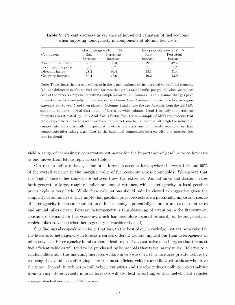
Table 9: Percent decrease in variance of household valuation of fuel economywhen imposing homogeneity in components of lifetime fuel costs

Gas price grows to t = 35 Gas price plateaus at t = 5Component Raw Persistent Raw Persistent

forecasts forecasts forecasts forecasts

Annual miles driven 33.7 37.3 39.7 42.4Local gasoline price 0.5 0.7 1.1 1.2Discount factor 28.3 36.4 48.1 51.4Gas price forecast 60.4 47.6 19.2 13.9

Note: Table shows the percent reduction in the logged variance of the marginal value of fuel economy

(i.e., the difference in lifetime fuel costs for cars that get 24 and 25 miles per gallon) when we replace

each of the various components with its sample-mean value. Columns 1 and 2 assume that gas price

forecasts grow exponentially for 35 years, while columns 3 and 4 assume that gas price forecasts grow

exponentially to year 5 and then plateau. Columns 1 and 3 take the raw forecasts from the full MSC

sample to be our empirical distribution of forecasts, while columns 2 and 4 use only the persistent

forecasts (as estimated by individual fixed effects) from the sub-sample of MSC respondents that

are surveyed twice. Percentages in each column do not sum to 100 because, although the individual

components are statistically independent, lifetime fuel costs are not linearly separable in these

components after taking logs. That is, the individual components interact with one another. See

text for details.

yield a range of increasingly conservative estimates for the importance of gasoline price forecastsas one moves from left to right across table 9.

Our results indicate that gasoline price forecasts account for anywhere between 14% and 60%of the overall variance in the marginal value of fuel economy across households. We suspect thatthe “right” answer lies somewhere between these two extremes. Annual miles and discount ratesboth generate a large, roughly similar amount of variance, while heterogeneity in local gasolineprices explains very little. While these calculations should only be viewed as suggestive given thesimplicity of our analysis, they imply that gasoline price forecasts are a potentially important sourceof heterogeneity in consumer valuation of fuel economy—potentially as important as discount ratesand annual miles driven. Forecast heterogeneity is thus deserving of attention in the literature onconsumers’ demand for fuel economy, which has heretofore focused primarily on heterogeneity invehicle miles traveled (when heterogeneity is considered at all).

Our findings also speak to an issue that has, to the best of our knowledge, not yet been raised inthe literature: heterogeneity in forecasts carries different welfare implications than heterogeneity inmiles traveled. Heterogeneity in miles should lead to positive assortative matching, so that the mostfuel efficient vehicles will tend to be purchased by households that travel many miles. Relative to arandom allocation, this matching increases welfare in two ways. First, it increases private welfare byreducing the overall cost of driving, since the most efficient vehicles are allocated to those who drivethe most. Second, it reduces overall vehicle emissions and thereby reduces pollution externalitiesfrom driving. Heterogeneity in price forecasts will also lead to sorting, so that fuel efficient vehicles

a sample standard deviation of 4.2% per year.

29

will be purchased by households with relatively high future price forecasts. This sorting, however,does not lead to welfare benefits because it reduces neither the total cost of driving nor totalemissions. In fact, sorting based on forecast heterogeneity can act as noise that leads to less thanperfect sorting on miles traveled, thereby reducing welfare rather than improving it. The extentto which this occurs depends on the relative variances of miles traveled and price forecasts in thepopulation. We believe our findings here provide useful initial evidence on this issue.

9 Conclusion

Do consumers exhibit a reasonable forecast of future energy prices? Our analysis suggests that theydo, at least in the important case of gasoline. Using two decades of high-quality survey data fromthe Michigan Survey of Consumers, we find that consumers, on average, report forecasts that areconsistent with a real no-change model of future gasoline prices, which recent research suggests isa sensible benchmark. Thus, if average consumers do undervalue fuel economy, the undervaluationlikely does not stem from consumers having systematic bias in their beliefs about energy prices.

How should future research model consumer forecasts of energy prices? Our analysis providessubstantial guidance. Researchers are likely to be justified in assuming that average consumersemploy a no-change forecast in most circumstances. The deviation from the no-change forecastduring the financial crisis of 2008, however, implies that researchers should use caution when es-timating demand for automobiles as a function of current gasoline prices during this time period.Estimates will likely be improved by assuming consumers forecast mean reversion in this window.More generally, if the deviation from the no-change forecast during the crisis was driven by con-sumers perceiving the deep recession and consequent drop in gasoline prices to be temporary, itmay be more accurate to model consumer forecasts as mean-reverting during other steep economicdownturns that trigger precipitous gasoline price declines.

Researchers should also be attentive to heterogeneity in forecasts, which we show is substantialand potentially as important as other sources of heterogeneity in generating variation in consumers’valuation of fuel economy. Little of this heterogeneity can be explained with common demographicfactors, which implies that residual variation will be large even when a rich set of controls areavailable. Importantly, the amount of forecast heterogeneity is increasing with the current gasolineprice when measured in levels, but it is roughly constant in logs.

Our results also provide guidance on how different sources of identifying variation will affectforecasts. Our state panel analysis suggests that consumers cannot easily distinguish betweenstate-specific gasoline price shocks and the national time series. That is, while consumers respondsomewhat less to state-specific shocks, consumers predict far more persistence than is consistentwith historical price data. Our analysis of the relative impact of tax changes versus pre-tax pricechanges on consumer forecasts fails to support the notion that consumers respond more strongly togasoline tax changes, perhaps because taxes are not salient in this market, where all posted pricesare tax-inclusive.

30

Throughout the paper we used the case of demand for fuel economy in autombiles to illustratethe implications of our findings, but our results should prove useful well beyond the specific litera-ture on consumer valuation of energy efficiency. Virtually all research involving consumer responsesto energy prices requires assumptions about how consumers forecast future prices, including modelsof search, models of demand for energy-using durables, and studies of the macroeconomic effectsof energy price shocks. We believe that the stylized facts established here regarding the natureof consumer beliefs about gasoline prices will improve these various literatures, as well as serve asan important data point for the more general question of how consumers forecast future economicoutcomes like inflation and growth.

References

Allcott, Hunt, “The Welfare Effects of Misperceived Product Costs: Data and Calibrations fromthe Automobile Market,” January 2012. Manuscript: NYU.

and Nathan Wozny, “Gasoline Prices, Fuel Economy, and the Energy Paradox,” July 2011.Manuscript: MIT.

, Sendhil Mullainathan, and Dmitry Taubinsky, “Externalities, Internalities, and theTargeting of Energy Policy,” April 2012. NBER Working Paper 17977.

Alquist, Ron and Lutz Kilian, “What Do We Learn From the Price of Crude Oil Futures?,”Journal of Applied Econometrics, June/July 2010, 25 (4), 539–573.

, , and Robert J. Vigfusson, “Forecasting the Price of Oil,” in Graham Elliot and AllanTimmerman, eds., Handbook of Economic Forecasting, Vol. Forthcoming, Elsevier, 2010.

Anderson, Soren T. and James M. Sallee, “Using Loopholes to Reveal the Marginal Costof Regulation: The Case of Fuel-Economy Standards,” American Economic Review, June 2011,101 (4), 1375–1409.

, Ryan Kellogg, James M. Sallee, and Richard T. Curtin, “Forecasting Gasoline PricesUsing Consumer Surveys,” American Economic Review Papers & Proceedings, May 2011, 101(3), 110–114.

Bento, Antonio M., Shanjun Li, and Kevin Roth, “Is There an Energy Paradox in FuelEconomy? A Note on the Role of Consumer Heterogeneity and Sorting Bias,” Economics Letters,April 2012, 115 (1), 44–48.

Berry, Steven, James Levinsohn, and Ariel Pakes, “Automobile Prices in Market Equilib-rium,” Econometrica, July 1995, 64 (4), 841–890.

Busse, Meghan R., Christopher R. Knittel, and Florian Zettelmeyer, “Are ConsumersMyopic? Evidence from New and Used Car Purchases,” American Economic Review, Forthcom-ing.

31

Curtin, Richard, “”Inflation Expectations and Empirical Tests: Theoretical Models and Em-pirical Tests”,” in Peter Sinclair, ed., Inflation Expectations, Vol. 56, New York: RoutledgeInternational Studies in Money and Banking, 2010, pp. 34–61.

Curtin, Richard T., “Pyschology and Macroeconomics,” in Robert L. Kahn, F. Thomas Juster,James S. House, Howard Schuman, and Eleanor Singer, eds., A Telescope on Society: SurveyResearch and Social Science at the University of Michigan & Beyond, Ann Arbor: University ofMichigan Press, 2004.

Davis, Lucas W. and Lutz Kilian, “Estimating the Effect of a Gasoline Tax on Carbon Emis-sions,” Journal of Applied Econometrics, 2011, 26, 1187–1214.

Dubin, Jeffrey A. and Daniel L. McFadden, “An Econometric Analysis of Residential ElectricAppliance Holdings and Consumption,” Econometrica, March 1984, 52 (2), 345–362.

Elliott, Graham, Thomas J. Rothenberg, and James H. Stock, “Efficient Tests for anAutoregressive Unit Root,” Econometrica, July 1996, 64 (4), 813–836.

Gillingham, Kenneth, “How Do Consumers Respond to Gasoline Price Shocks? Heterogeneityin Vehicle Choice and Driving Behavior,” March 2011. Manuscript: Yale University.

Goldberg, Pinelopi Koujianou, “The Effects of the Corporate Average Fuel Efficiency Stan-dards in the U.S.,” The Journal of Industrial Economics, March 1998, 46 (1), 1–33.

Hamilton, James D., “Oil and the Macroeconomy,” in Steven N. Durlauf and Lawrence E.Blume, eds., The New Palgrave Dictionary of Economics, 2nd ed., Palgrave Macmillan, 2008.

, “Understanding Crude Oil Prices,” The Energy Journal, 2009, 30 (2), 179–206.

Hastings, Justine S. and Jesse Shapiro, “Mental Accounting and Consumer Choice: Evidencefrom Commodity Price Shocks,” April 2011. Manuscript: University of Chicago.

Kahn, James A., “Gasoline Prices and the Used Automobile Market: A Rational ExpectationsAsset Price Approach,” The Quarterly Journal of Economics, 1986, 101 (2), 323–339.

Kilian, Lutz and Eric R. Sims, “The Effects of Real Gasoline Prices on Automobile Demand:A Structural Analysis Using Micro Data,” April 2006. Manuscript: University of Michigan.

Klier, Thomas and Joshua Linn, “New Vehicle Characteristics and the Cost of the CorporateAverage Fuel Economy Standard,” December 2010. Resources for the Future Discussion Paper10-50.

Knittel, Christopher R. and Ryan Sandler, “Carbon Prices and Automobile Greenhouse GasEmissions: The Extensive and Intensive Margins,” in Don Fullerton and Catherine Wolfram,eds., The Design and Implementation of U.S. Climate Policy, NBER, Forthcoming.

32

Langer, Ashley and Nathan H. Miller, “Automakers’ Short-Run Responses to ChangingGasoline Prices and the Implications for Energy Policy,” August 2011. Manuscript: Universityof Michigan.

Lewis, Matthew and Howard P. Marvel, “When Do Consumers Search?,” Journal of IndustrialEconomics, September 2011, 59 (3), 457–483.

Li, Shanjun, Christopher Timmins, and Roger H. von Haefen, “How Do Gasoline PricesAffect Fleet Fuel Economy?,” American Economic Journal: Economic Policy, August 2009, 1(2), 113–137.

, Joshua Linn, and Erich Muehlegger, “Gasoline Taxes and Consumer Behavior,” February2012. Manuscript: Harvard University.

Linn, Joshua and Thomas Klier, “The Price of Gasoline and New Vehicle Fuel Economy:Evidence from Monthly Sales Data,” American Economic Journal: Economic Policy, August2010, 2 (3), 134–153.

Lu, S., “Vehicle Survivability and Travel Mileage Schedules,” Technical Report DOT HS 809 952,National Highway Traffic Safety Administration January 2006.

Mankiw, N. Gregory, Ricardo Reis, and Justin Wolfers, “Disagreement about InflationExpectations,” in Mark Gertler and Kenneth Rogoff, eds., NBER Macroeconomics Annual 2003,Vol. 18, Cambridge, MA: MIT Press, 2004, pp. 209–47.

Manski, Charles F., “Measuring Expectations,” Econometrica, September 2004, 72 (5), 1329–1376.

Ng, Serena and Pierre Perron, “Lag Length Selection and the Construction of Unit Root Testswith Good Size and Power,” Econometrica, November 2001, 69 (6), 1519–1554.

Sallee, James M., Sarah E. West, and Wei Fan, “Consumer Valuation of Fuel Economy:A Microdata Approach,” Proceedings of the National Tax Association Annual Conference onTaxation, 2009.

Small, Kenneth A. and Kurt Van Dender, “Fuel Efficiency and Motor Vehicle Travel: TheDeclining Rebound Effect,” Energy Journal, 2007, 28 (1), 25–51.

van der Klaauw, Wilbert, Wandi Bruine de Bruin, Giorgio Topa, Simon Potter, and

Michael Bryan, “Rethinking the Measurement of Household Inflation Expectations: Prelimi-nary Findings,” December 2008. Federal Reserve Bank of New York Staff Report No. 359.

West, Sarah E. and Roberton C. Williams III, “Optimal Taxation and Cross-Price Effectson Labor Supply: Estimates of the Optimal Gas Tax,” Journal of Public Economics, April 2007,91, 593–617.

33

Whitefoot, Katie, Meredith Fowlie, and Steven Skerlos, “Evaluating U.S. Reformed Cor-porate Average Fuel Economy Standards using an Engineering Attribute Selection Model,” De-cember 2011. Manuscript: University of California, Berkeley.

Appendix

Table A1 presents summary statistics for the sample of 77,144 individual MSC respondents withnon-missing values for both gasoline price and inflation forecasts during 1993–2009.

Table A1: Summary statistics for individual response data

Variable Mean Std. Dev. Minimum Maximum

Real, levelsForecast gas price 2.123 0.958 0.182 13.923Current gas price 2.073 0.660 1.164 4.519Forecast gas price change 0.050 0.629 -3.040 11.596Real, logsForecast gas price 0.668 0.403 -1.704 2.634Current gas price 0.684 0.290 0.151 1.508Forecast gas price change -0.016 0.255 -2.062 2.081Nominal, levelsForecast gas price 2.175 1.146 0.188 12.046Current gas price 1.799 0.752 0.919 4.423Forecast gas price change 0.376 0.651 -3.000 9.950Nominal, logsForecast gas price 0.664 0.457 -1.671 2.489Current gas price 0.510 0.383 -0.084 1.487Forecast gas price change 0.154 0.211 -1.962 1.913Nominal, percent per yearForecast rate of gas price change 0.032 0.045 -0.325 0.466Forecast inflation rate 0.035 0.037 -0.330 0.500

Note: Table reports summary statistics for sample of 77,144 individual MSC respondents with non-missing

values for both gasoline price and inflation forecasts during 1993–2009, weighted by their individual MSC

sampling weights. See text for details on construction of these variables. At bottom, the forecasted rate

of gasoline price increase is given by (1 + C60it /Pit)

1/5−1, where C60it is the respondent’s forecasted change

over five years and Pit is the current price, both in nominal terms. The forecasted inflation rate is reported

directly by survey respondents.

Figures A1 and A2 provide corollaries to figures 3 and 4 using logged values. Specifically, welog the individual values of the nominal and real gasoline price forecasts and then average acrossobservations. These averages are used to generate the “Logs” results in tables 2, 3, and 4.

34

Figure A1: Nominal gasoline prices and forecasts in logs.

−.5

0.5

11

.52

$/g

allo

n,

no

min

al (lo

gs)


Date

Mean forecast

Current price


Figure A2: Real gasoline prices and forecasts in logs.

−.5

0.5

11

.52

$/g

allo

n,

rea

l (lo

gs)


Date

Mean forecast

Current price


35

revised version published in journal of environmental...

Documents