Response of structure subjected to different

Earthquake Ground Motions

A Thesis Submitted in Partial Fulfillment of the Requirements for the

Degree of

Bachelor of Technology

In

Civil Engineering

By: Under the Supervision of:

Ahmad Milad Prof. Pradip Sarkar

Roll No: 111CE0554

DEPARTMENT OF CIVIL ENGINEERING

NATIONAL INSTITUTE OF TECHNOLOGY,

ROURKELA-769008(INDIA)

JULY 2015

I

NATIONAL INSTITUTE OF TECHNOLOGY

ROURKELA, ORISSA-769008, INDIA

CERTIFICATE

This is to certify that this thesis entitled “RESPONSE OF STRUCTURE SUBJECTED TO

DIFFERENT EARTHQUAKE GROUND MOTIONS” submitted by Ahmad Milad

(111CE0554) in partial fulfillment for the award of the degree of Bachelor of Technology in

Civil Engineering at National Institute of Technology, Rourkela is an authentic work carried out

by him under my supervision.

To the best of my knowledge, the matter embodied in this report has not been submitted to any

other university/institute for the award of any degree or diploma.

Date: - July-2015

Prof. Pradip Sarkar

(Project Supervisor)

Department of Civil Engineering,

National Institute of Technology Rourkela,

Rourkela-769008, Odisha, India

II

ACKNOWLEDGEMENT

First and foremost, praise and thanks goes to my Allah for the blessing that has bestowed upon

me in all my endeavors. The satisfaction and ecstasy on the successful completion of any task

would be imperfect without the mention of the people who made it possible whose endless

guidance and encouragement crowned my effort with success.

I would like to express my heartfelt appreciation to my esteemed supervisor Prof. Pradip

Sarkar for his technical guidance, valuable suggestions, and encouragement throughout the

analytical study and in preparing this thesis. It has been an honour to work under Prof. Pradip

Sarkar whose expertise and discernment were key in the accomplishment of this project.

I am grateful to the Dept. of Civil Engineering, NIT ROURKELA, for giving me the chance

to execute this project, which is an integral part of the curriculum in B.Tech program at the

National Institute of Technology, Rourkela. Many thanks to my friends who directly or

indirectly helped me in my project work for their substantial contribution towards enriching the

quality of the work.

I would also thank members of Department of Civil Engineering, NIT, Rourkela and academic

staffs of this department for their extended assistance. This acknowledgement would not be

complete without expressing my sincere gratitude to my parents, brothers and sisters for their

love, patience, encouragement, and understanding. My Parents are the source of my enthusiasm

and inspiration throughout my work. Finally I would like to dedicate my work and this thesis to

my parents.

Ahamd Milad

B.Tech, Department of Civil Engineering

National Institute of Technology Rourkela,

Rourkela-769008, Odisha, India

III

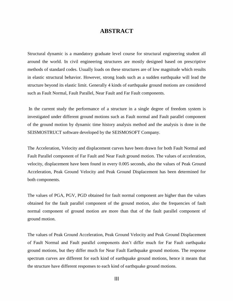
ABSTRACT

Structural dynamic is a mandatory graduate level course for structural engineering student all

around the world. In civil engineering structures are mostly designed based on prescriptive

methods of standard codes. Usually loads on these structures are of low magnitude which results

in elastic structural behavior. However, strong loads such as a sudden earthquake will lead the

structure beyond its elastic limit. Generally 4 kinds of earthquake ground motions are considered

such as Fault Normal, Fault Parallel, Near Fault and Far Fault components.

In the current study the performance of a structure in a single degree of freedom system is

investigated under different ground motions such as Fault normal and Fault parallel component

of the ground motion by dynamic time history analysis method and the analysis is done in the

SEISMOSTRUCT software developed by the SEISMOSOFT Company.

The Acceleration, Velocity and displacement curves have been drawn for both Fault Normal and

Fault Parallel component of Far Fault and Near Fault ground motion. The values of acceleration,

velocity, displacement have been found in every 0.005 seconds, also the values of Peak Ground

Acceleration, Peak Ground Velocity and Peak Ground Displacement has been determined for

both components.

The values of PGA, PGV, PGD obtained for fault normal component are higher than the values

obtained for the fault parallel component of the ground motion, also the frequencies of fault

normal component of ground motion are more than that of the fault parallel component of

ground motion.

The values of Peak Ground Acceleration, Peak Ground Velocity and Peak Ground Displacement

of Fault Normal and Fault parallel components don’t differ much for Far Fault earthquake

ground motions, but they differ much for Near Fault Earthquake ground motions. The response

spectrum curves are different for each kind of earthquake ground motions, hence it means that

the structure have different responses to each kind of earthquake ground motions.

IV

TABLE OF CONTENTS

TITLE PAGE NO.

Certificate………………………………………………………………………………….. I

Acknowledgement………………………………………………………………………… II

Abstract……………………………………………………………………...................... III

List of Figures …………………………………………………………………………... VII

List of Tables………………………………………………………………......................VII

List of Graphs……………………………………………………………………….….. VIII

Notation and Abbreviations…………………………………………………...................... X

CHAPTER 1

1. ITRODUCTION …………………………………………….……….1

1.1 General …………………………………………………………………………2

1.2 Seismic waves ………………………………………………………………….3

1.3 Fault ………………………………………………………………………….…3

1.3.1 Fault Parallel Earthquake …………………………………………….…5

1.3.2 Fault Normal Earthquake …………………………………………….…5

1.3.3 Near Fault Earthquake ……………………………………………….…6

1.3.4 Far Fault Earthquake …………………………………………………...6

1.4 Objective and Scope ……………………………………………………….…..7

1.5 Methodology ………………………………………………………………..….8

CHAPTER 2

2. LITERATURE REVIEW …………………………..…....…………9

2.1 General ………………………………………………………………….….....10

2.2 Summary of literature Review ………………….…………………………….13

V

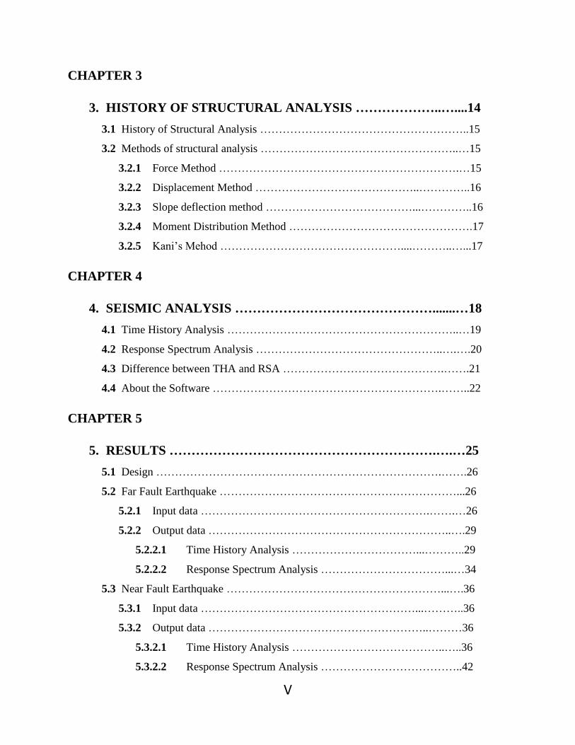
CHAPTER 3

3. HISTORY OF STRUCTURAL ANALYSIS ………………..…....14

3.1 History of Structural Analysis ………………………………………………..15

3.2 Methods of structural analysis ……………………………………………..…15

3.2.1 Force Method ……………………………………………………….…15

3.2.2 Displacement Method ……………………………………..…………..16

3.2.3 Slope deflection method …………………………………...…………..16

3.2.4 Moment Distribution Method ………………………………………….17

3.2.5 Kani’s Mehod …………………………………………....………..…...17

CHAPTER 4

4. SEISMIC ANALYSIS ……………………………………….......…18

4.1 Time History Analysis ……………………………………………………..…19

4.2 Response Spectrum Analysis …………………………………………..….….20

4.3 Difference between THA and RSA …………………………………….…….21

4.4 About the Software …………………………………………………….……..22

CHAPTER 5

5. RESULTS …………………………………………………….….…25

5.1 Design ………………………………………………………………….…….26

5.2 Far Fault Earthquake ………………………………………………………...26

5.2.1 Input data …………………………………………………….…….…26

5.2.2 Output data ………………………………………………………..….29

5.2.2.1 Time History Analysis ……………………………...………..29

5.2.2.2 Response Spectrum Analysis ……………………………...…34

5.3 Near Fault Earthquake …………………………………………………...….36

5.3.1 Input data …………………………………………………...………..36

5.3.2 Output data …………………………………………………..………36

5.3.2.1 Time History Analysis …………………………………..…..36

5.3.2.2 Response Spectrum Analysis ………………………………..42

VI

CHAPTER 6

6. SUMMARY AND CONCLUSION …………………………….…...44

6.1 Summary …………………………………………………………….…….……45

6.2 Conclusion …………………………………………………………….….….....45

CHAPTER 7

7. REFERENCES …………………………………………………..…...46

7.1 References……………………………………………………………………….47

VII

LIST OF FIGURES

FIG NO. NAME OF FIGURE PAGE NO.

1.1 Fault plane 5

1.2 Epicenter and Focus of the earthquake 6

1.3 Near Field and Far Field Earthquake Ground Motion 7

5.1 Single Degree of Freedom Model designed in SEISMOSTRUCT 26

5.2 PEER Strong Motion Database 27

LIST OF TABLES

TABLE NO. NAME OF TABLE PAGE NO.

5.1 Earthquake and Station Details 27

5.2 Downloaded Input data 28

5.3 Far Fault earthquake results 34

5.4 Near Fault earthquake results 42

VIII

LIST OF GRAPHS

GRAPH NO. NAME OF GRAPH PAGE NO.

5.1 Acceleration curve (Fault Normal & fault parallel Input data)

for Far Fault Earthquake

28

5.2 Acceleration curve (Fault Normal & fault parallel) for Far Fault

Earthquake

29

5.3 Acceleration curve (Fault Normal) for Far Fault Earthquake 30

5.4 Acceleration curve (Fault Parallel) for Far Fault Earthquake 30

5.5 Velocity Curve (Fault Normal & Fault Parallel) for Far Fault

Earthquake

31

5.6 Velocity Curve (Fault Normal) for Far Fault Earthquake 31

5.7 Velocity curve (Fault parallel) for Far Fault Earthquake 32

5.8 Displacement Curve (Fault Normal & Fault Parallel) for Far

Fault Earthquake

32

5.9 Displacement Curve (Fault Normal) for Far Fault Earthquake 33

5.10 Displacement Curve (Fault Parallel) for Far Fault Earthquake 33

5.11 Response spectrum curve (Fault normal) for Far Fault

Earthquake

34

5.12 Response spectrum curve (Fault parallel) for Far Fault

Earthquake

35

5.13 Acceleration curve (Fault Normal & fault parallel Input data)

for Near Fault Earthquake

36

5.14 Acceleration curve (Fault Normal & fault parallel) for Near

Fault Earthquake

37

5.15 Acceleration curve (Fault Normal) for Near Fault Earthquake 38

5.16 Acceleration curve (Fault Parallel) for Near Fault Earthquake 38

IX

GRAPH NO. NAME OF GRAPH PAGE NO.

5.17 Velocity Curve (Fault Normal & Fault Parallel) for Near Fault

Earthquake

39

5.18 Velocity Curve (Fault Normal) for Near Fault Earthquake 39

5.19 Velocity curve (Fault parallel) for Near Fault Earthquake 40

5.20 Displacement Curve (Fault Normal & Fault Parallel) for Near

Fault Earthquake

40

5.21 Displacement Curve (Fault Normal) for Near Fault Earthquake 41

5.22 Displacement Curve (Fault Parallel) for Near Fault Earthquake 41

5.23 Response spectrum curve (Fault normal) for Near Fault

Earthquake

42

5.24 Response spectrum curve (Fault parallel) for Near Fault

Earthquake

43

X

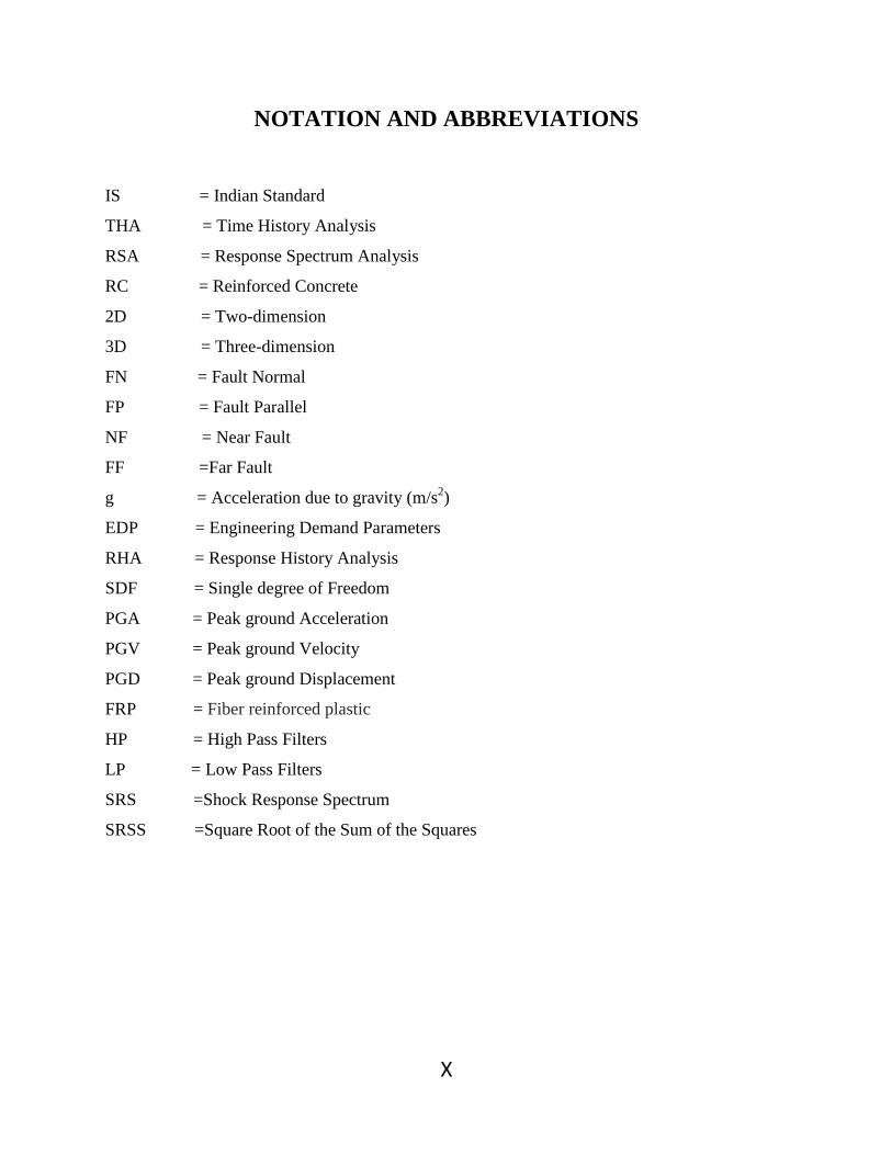
NOTATION AND ABBREVIATIONS

IS = Indian Standard

THA = Time History Analysis

RSA = Response Spectrum Analysis

RC = Reinforced Concrete

2D = Two-dimension

3D = Three-dimension

FN = Fault Normal

FP = Fault Parallel

NF = Near Fault

FF =Far Fault

g = Acceleration due to gravity (m/s2)

EDP = Engineering Demand Parameters

RHA = Response History Analysis

SDF = Single degree of Freedom

PGA = Peak ground Acceleration

PGV = Peak ground Velocity

PGD = Peak ground Displacement

FRP = Fiber reinforced plastic

HP = High Pass Filters

LP = Low Pass Filters

SRS =Shock Response Spectrum

SRSS =Square Root of the Sum of the Squares

1

CHAPTER 1

INTRODUCTION

2

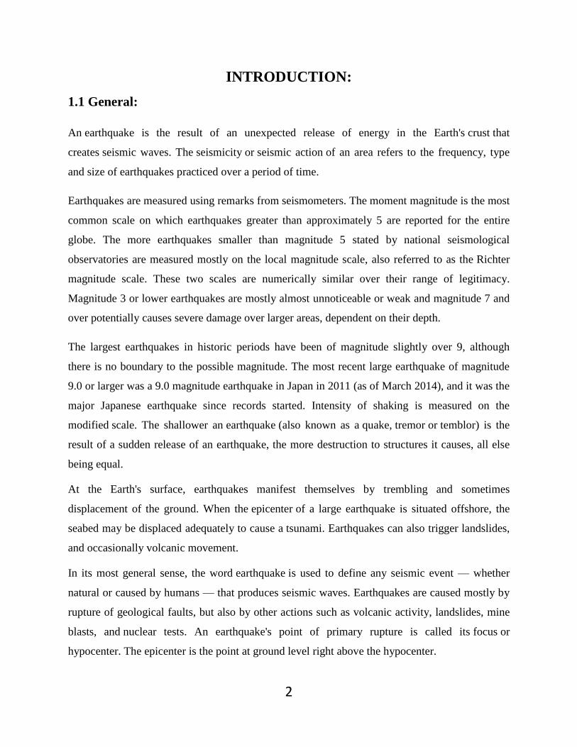
INTRODUCTION:

1.1 General:

An earthquake is the result of an unexpected release of energy in the Earth's crust that

creates seismic waves. The seismicity or seismic action of an area refers to the frequency, type

and size of earthquakes practiced over a period of time.

Earthquakes are measured using remarks from seismometers. The moment magnitude is the most

common scale on which earthquakes greater than approximately 5 are reported for the entire

globe. The more earthquakes smaller than magnitude 5 stated by national seismological

observatories are measured mostly on the local magnitude scale, also referred to as the Richter

magnitude scale. These two scales are numerically similar over their range of legitimacy.

Magnitude 3 or lower earthquakes are mostly almost unnoticeable or weak and magnitude 7 and

over potentially causes severe damage over larger areas, dependent on their depth.

The largest earthquakes in historic periods have been of magnitude slightly over 9, although

there is no boundary to the possible magnitude. The most recent large earthquake of magnitude

9.0 or larger was a 9.0 magnitude earthquake in Japan in 2011 (as of March 2014), and it was the

major Japanese earthquake since records started. Intensity of shaking is measured on the

modified scale. The shallower an earthquake (also known as a quake, tremor or temblor) is the

result of a sudden release of an earthquake, the more destruction to structures it causes, all else

being equal.

At the Earth's surface, earthquakes manifest themselves by trembling and sometimes

displacement of the ground. When the epicenter of a large earthquake is situated offshore, the

seabed may be displaced adequately to cause a tsunami. Earthquakes can also trigger landslides,

and occasionally volcanic movement.

In its most general sense, the word earthquake is used to define any seismic event — whether

natural or caused by humans — that produces seismic waves. Earthquakes are caused mostly by

rupture of geological faults, but also by other actions such as volcanic activity, landslides, mine

blasts, and nuclear tests. An earthquake's point of primary rupture is called its focus or

hypocenter. The epicenter is the point at ground level right above the hypocenter.

3

1.2 Seismic waves:

Seismic waves are waves of energy that travel through the Earth's layers, and are an outcome of

an earthquake, explosion, or a volcano that imparts low-frequency acoustic energy. Many other

natural and anthropogenic sources create low amplitude waves commonly stated to as ambient

vibrations. Seismic waves are studied by geophysicists called seismologists. Seismic wave fields

are noted by a seismometer, hydrophone (in water), or accelerometer.

The propagation speed of the waves depends on density and elasticity of the medium. Velocity

tends to rise with depth, and ranges from approximately 2 to 8 km/s in the Earth's crust up to

13 km/s in the deep mantle.

Earthquakes generate various types of waves with different velocities; when getting seismic

observatories, their different travel time help scientists to trace the source of the

earthquake hypocenter. In geophysics the refraction or reflection of seismic waves is used for

investigation into the structure of the Earth's interior, and man-made vibrations are regularly

generated to investigate shallow, subsurface structures.

1.3 Fault:

A fault is a planar fracture in a volume of rock, across which there has been substantial

displacement along the fractures as a consequence of earth movement. Large faults inside the

Earth's crust result from the action of plate tectonic forces, with the prime forming the

boundaries between the plates, such as subduction zones or renovate faults. Energy release

associated with rapid movement on active faults is the origin of most earthquakes.

A fault line is the surface trace of a fault, the line of connection between the fault plane and the

Earth's surface.

Since faults do not generally consist of a single, clean fracture, geologists use the term fault

zone when referring to the zone of complex deformation allied to the fault plane.

4

The two sides of a non-vertical fault are known as the hanging wall and footwall. By definition,

the hanging wall occurs overhead the fault plane and the footwall occurs beneath the fault. This

terminology arises from mining.

Because of friction and the rigidity of the rock, the rocks cannot slide or flow past each other.

Rather, stress builds up in rocks and when it reaches a level that go beyond the strain threshold,

the accumulated potential energy is dissipated by the relief of strain, which is focused into a

plane along which relative motion is accommodated—the fault. Strain is both accumulative and

instantaneous depending on the rheology of the rock; the ductile lower crust and mantle stores

deformation gradually via shearing, while the brittle upper crust reacts by fracture -

instantaneous stress release - to cause motion along the fault. A fault in ductile rocks can

moreover release instantaneously when the strain rate is too great. The energy released by

instantaneous strain release causes earthquakes, a common phenomenon along transform

boundaries.

In the earlier ages structures were only designed for gravity loads and lateral load were not taken

in consideration, then when the structure was subjected to lateral loads such as wind load and

earthquake loads then it was getting damaged, so the engineers decided to make wind resistant

and earthquake resistant structures.

In here we will be talking about earthquake resistant structures, and for doing such we need the

ground acceleration data for the site where the structure is located and then we will prepare the

design according to the ground acceleration history data.

In this research we will be taking 4 kinds of earthquakes mentioned below:

1. Far Fault Earthquake

1a. Fault Parallel component

1b. Fault Normal component

2. Near Fault Earthquake

2a. Fault Parallel component

2b. Fault Normal component

5

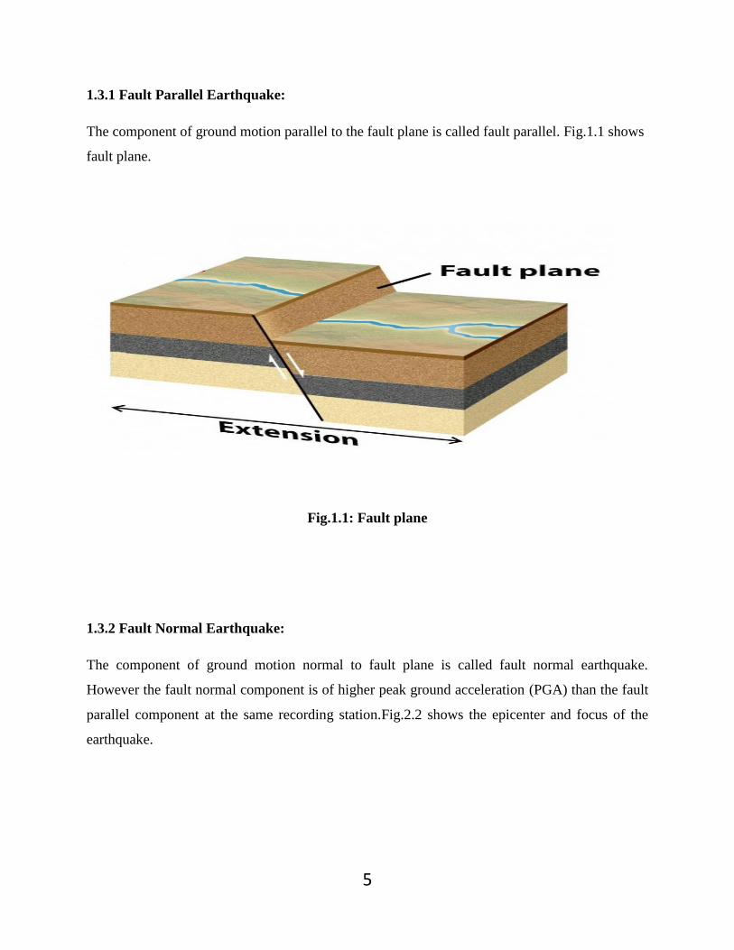
1.3.1 Fault Parallel Earthquake:

The component of ground motion parallel to the fault plane is called fault parallel. Fig.1.1 shows

fault plane.

Fig.1.1: Fault plane

1.3.2 Fault Normal Earthquake:

The component of ground motion normal to fault plane is called fault normal earthquake.

However the fault normal component is of higher peak ground acceleration (PGA) than the fault

parallel component at the same recording station.Fig.2.2 shows the epicenter and focus of the

earthquake.

6

Fig.1.2: Epicenter and Focus of the earthquake

1.3.3 Near Fault Earthquake:

When the site of the structure is near to the epicenter of the earthquake then it is called Near

Field Earthquake.

1.3.4 Far Fault Earthquake:

When the site where the structure is located is far from the epicenter of the earthquake then it is

called Far Field Earthquake; however there is no definite distance over which a site may be

classified as in near or far-field

.It is recognized that the characteristics of near-field earthquake ground motions are different

from those records in the far-field. Fig.1.3 shows the near field and far field earthquake.

The values of Peak Ground Acceleration, Peak Ground Velocity and Peak Ground Displacement

of Fault Normal and Fault parallel components don’t differ much for Far Fault earthquake

ground motions, but they differ much for Near Fault Earthquake ground motions.

7

Fig1.3: Near Field and Far Field Earthquake Ground Motion

1.4 Objective and Scope:

To study the differences in structural responses against different earthquake ground motions and

we compare the results as follows:

1. Far-field/Near-field

2. Fault-parallel/Fault-normal

To perform dynamic time history analysis on a structure in single degree of freedom system with

the use SEISMOSTRUCT software.

To compare the associated Response Spectrums for Fault Normal and Fault Parallel components

of both kinds of earthquake ground motions.

8

1.5 Methodology:

1. Studied Literature review for understanding the characteristics of different earthquake

ground motions.

2. Collected different earthquake ground motions from strong motion database.

3. Learned dynamic analysis of structures.

4. Learned response spectrum analysis.

5. Learned SEISMOSTRUCT software.

6. Modeled the structure (single degree of freedom system) in SEISMOSTRUCT software

and analyzed it for fault normal and fault parallel component of ground motion.

7. Compared the results (acceleration, displacement or velocity) for fault normal and fault

parallel component of far fault and near fault ground motion.

8. Compared the associated Response Spectrums.

9

CHAPTER 2

LITERATURE REVIEW

10

LITERATURE REVIEW:

2.1 General

Durgesh C. Rai (2005) has developed guidelines for seismic evaluation and firming up of

buildings. The document was established as part of project “Review of Building Codes and

Preparation of Commentary and Handbooks” presented to Indian Institute of Technology Kanpur

by the Gujarat State Disaster Management Authority (GSDMA), Gandhinagar through World

Bank finances. This document is predominantly concerned with the seismic evaluation and

strengthening of current buildings and it is proposed to be used as a guide.

Douglas Dreger, Gabriel Hurtado, Anil K. Chopra, Shawn Larsen, 2007 studied Near fault

seismic ground motion and got that For a vertical strike-slip fault the FN ground motions are the

same on each side of the fault, whereas the FP component doesn’t have equal amplitude but

contrary static offset. The corresponding velocity pulses are the equal on each side of the fault

for the FN component, but opposite in sign on the FP component. This degree of symmetry

vanishes when the fault is dipping due to the uncontrolled free-surface. Motions on the hanging

block side are greater due to the free-surface effect, and because a larger fraction of the fault

surface is nearer to the stations on the side of the fault that dips under the recording stations.

Kim and Elnashai (2009) observed that buildings for which seismic design was performed

using contemporary codes persisted the earthquake loads. However the vertical motion

significantly reduced the shear capacity in vertical members.

Abu Lego (2010) Site Response Spectra was used to study the response of buildings because of

earthquake loading. . According to the Indian standard for Earthquake resistant design (IS:

1893), the seismic force or base shear rest on on the zone factor (Z) and the average response

acceleration coefficient (Sa/g) of the soil kinds at thirty meter depth with suitable adjustment

depending upon the depth of foundation. In the present study an effort has been made to generate

response spectra using site definite soil parameters for some sites in Arunachal Pradesh and

Meghalay in seismic zone V and the generated response spectra is used to analyze some

structures using the design software STAAD Pro.

11

Mr. S. Yaghmaei-Sabegh and MR. N. Jalali-Milani, 2012 studied Pounding force response

spectrum for near-field and far-field earthquakes and got the result that insufficient separation

distance between neighboring buildings with out-of-phase response would rise the probability of

pounding during an earthquake and may cause serious damages to the structures. A rational

estimation of the maximum impact force would support us to control the extent of damages in

different structures. The pounding force response spectrum, which shows the value of maximum

impact force as a function of the structural vibration stages, is considered in this paper. It is well-

known that solid ground motion in the near-field area has different characteristics from far-field

ones. In this paper, pounding force response spectra for elastic structures subjected to near-field

and far-field ground motions are shown. Both of the neighboring buildings were modeled simply

as Single Degree Of Freedom (SDF) systems and pounding effect has been replicated by

applying the nonlinear viscoelastic model. In the analysis, the effect of altered parameters, such

as mass, damping ratio has been studied. The effects of gap distance on maximum pounding

force due to near- and far-field earthquake ground motions were studied comprehensively. As a

result, the characteristics of earthquake ground motions alongside with the properties of

structures should be considered in gap distance controlling amongst adjacent buildings.

Mr. J.C. Reyes and Mr. E. Kalkan, 2012 studied Relevance of Fault-Normal/Parallel and

Maximum Direction Rotated Ground Motions on Nonlinear Behavior of Multi-Story Buildings

and got that The existing state-of-practice in U.S. is to rotate the as-recorded couple of ground

motions to the fault normal and fault-parallel (FN/FP) directions before they are used as input for

three-dimensional nonlinear response history analyses (RHAs) of structures. It is presumed that

this approach will lead to two sets of responses that cover the range of possible responses over

all non-redundant rotation angles. Thus, it is considered to be a conservative method appropriate

for design verification of new structures. Based on the 9-story symmetric and asymmetric

buildings, the effect that the angle of rotation of the ground motion has on several engineering

demand parameters (EDPs) has been observed in nonlinear-inelastic domain.

12

Mr. Kalkan, and Mr. Kwong, 2012 studied Evaluation of fault-normal/fault-parallel directions

rotated ground motions for response history analysis of an instrumented six-story building and

got that depending on regulatory building codes in United States (for example, 2010 California

Building Code), at least two horizontal ground-motion components are required for three-

dimensional (3D) response history analysis (RHA) of structures. For sites within 5 km of an

active fault, these records should be divided to fault-normal/fault-parallel (FN/FP) directions,

and two RHA analyses should be performed individually (when FN and then FP are aligned with

the sloping direction of the structural axes). It is assumed that this tactic will lead to two sets of

responses that envelope the range of probable responses overall no redundant rotation angles.

This assumption is studied here using a 3D computer model of a six-story reinforced-concrete

instrumented building subjected to an ensemble of bidirectional near-fault ground motions. Peak

responses of engineering demand parameters (EDPs) were obtained for rotation angles ranging

from 0° through 180° for calculating the FN/FP directions. It is verified that rotating ground

motions to FN/FP directions (1) does not always lead to the maximum responses over all angles,

(2) does not always envelope the range of possible responses, and (3) does not provide maximum

responses for all EDPs instantaneously even if it provides a maximum response for a specific

EDP.

Yen-Po Wang (2014) introduced the basics of seismic base isolation as an effective technique

for seismic design of structures. Spring-like isolation bearings concentrated earthquake forces by

changing the fundamental time period of the structure so as to avoid resonance. Sliding-type

isolation bearings filter out the earthquake forces via discontinuous sliding interfaces and forces

were prohibited from getting transmitted to the superstructure due to the friction. The design of

the base isolation system involved finding out the base shear, bearing displacement etc. in

accordance with site-specific conditions.

13

3.2 Summary of literature Review:

1. The fault-normal component of numerous, but not all, near-fault ground motions carry

out much bigger deformation and strength demands compared to the fault-parallel

component over a wide range of vibration periods. In contrast, the two components of

most far-fault records are quite similar in their demands.

2. The strength and deformation demands of the fault-normal component of many near

fault ground motions are larger than that of the fault-parallel component primarily

because the peak acceleration, velocity and displacement of the previous are much

larger, although its response amplification factors are lesser.

3. The velocity-sensitive spectral region for the fault-normal component of near-fault

records is much thinner, and their acceleration-sensitive and displacement-sensitive

regions are much broader, compared to far-fault motions. The narrower velocity-

sensitive region of near-fault records is shifted to lengthier periods.

4. For the same ductility factor, near-fault ground motions impose a higher strength

demand in their acceleration-sensitive region compared to far-fault motions, with both

demands stated as a fraction of their respective elastic demands. This systematic

difference is primarily because of the difference between the Tc values for the two sorts

of excitations. If the period scale is normalized relative to the Tc value, the strength

reduction factors for the two types of motions are similar over all spectral regions.

14

CHAPTER 3

HISTORY OF

STRUCTURAL

ANALYSIS

15

3.1 History of Structural Analysis

A structure refers to a system of two or more connected parts used to resist a load. It may be

considered as a gathering of two or more basic components linked to each other so that they

carry the design loads securely without causing any serviceability failure. Once initial design of a

structure is fixed, the structure then must be analyzed to make sure that it has its essential

strength and rigidity. The loadings are supposed to be taken from particular design codes and

local specifications, if any. The forces in the members and the displacements of the joints are

found using the theory of structural analysis. The entire structural system and its loading

conditions might be of complex nature, so to make the analysis easier, certain simplifying

assumptions associated to the material quality, member geometry, nature of applied loads, their

distribution, the type of connections at the joints and the support conditions are used. This shall

assist making the process of structural analysis simpler to quite an extent.

3.2 Methods of structural analysis

When the number of unknown reactions or the number of internal forces surpasses the

number of equilibrium equations existing for the purpose of analysis, the structure is called a

statically indeterminate structure. Many structures are statically indeterminate. This

indeterminacy may be as a result of additional supports or extra members, or by the general form

of the structure. While analyzing any indeterminate structure, it is important to satisfy

equilibrium, compatibility, and force-displacement conditions for the structure. The fundamental

methods to analyze the statically indeterminate structures are discussed below.

3.2.1 Force method

The force method developed first by James Clerk Maxwell and further developed later by

Otto Mohr and Heinrich Muller-Breslau was one of the first methods available for analysis of

statically indeterminate structures. This method is also known as compatibility method or the

method of consistent displacements. In this method, the compatibility and force displacement

requirements for the particular structure are first defined in order to determine the redundant

forces. Once these forces are determined, the remaining reactive forces on the given structure are

found out by satisfying the equilibrium requirements.

16

3.2.2 Displacement method

In the displacement method, first of all load-displacement relations for the members of the

structure are determined and then the equilibrium requirements for the same are satisfied. The

unknowns in the equations are displacements. Unknown displacements are written in terms of

the loads or forces by using the load-displacement relations and then these equations are solved

to find out the displacements. As the displacements are found out, the loads are determined from

the compatibility and load- displacement equations. Some classical techniques used to apply the

displacement method are discussed.

3.2.3 Slope deflection method

This method was first invented by Heinrich Manderla and Otto Mohr to study the secondary

stresses in trusses and was after developed by G. A. Maney in order to extend its application to

analyze indeterminate beams and framed structures. The basic assumption of this technique is to

consider the deformations caused only by bending moments. It is supposed that the effects of

shear force or axial force deformations are negligible in indeterminate beams or frames. The

fundamental slope-deflection equation states the moment at the end of a member as the

superposition of the end moments caused due to the external loads on the member, with the ends

being assumed as restrained, and the end moments caused by the displacements and actual end

rotations. Slope-deflection equations are applied to every member of the structure. Using proper

equations of equilibrium for the joints along with the slope-deflection equations of each member,

a set of simultaneous equations with unknowns as the displacements are obtained. Once the

values of these displacements are determined, the end moments are found using the slope-

deflection equations.

17

3.2.4 Moment distribution method

This method of analyzing beams and multi-storey frames using moment distribution was

presented by Prof. Hardy Cross in 1930, and is also sometimes known as Hardy Cross method. It

is an iterative method. Initially all the joints are temporarily restrained against rotation and fixed

end moments for each of the member are written down. Every joint is then released one by one

in succession and the unbalanced moment is distributed to the ends of the members in the ratio of

their distribution factors. These distributed moments are then carried over to the far ends of the

joints. Again the joint is temporarily restrained before going to the next joint. Same set of

operations are done at each joint till all the joints are completed and the results achieved are up to

desired accuracy. The method does not involve solving a number of simultaneous equations,

which may get pretty complicated while dealing with large structures, and is thus preferred over

the slope-deflection method.

3.2.5 Kani’s method

This method was first established by Prof. Gasper Kani of Germany in the year 1947.

This is an indirect extension of slope deflection method. This is an effective method due to

simplicity of moment distribution. The method offers an iterative scheme for applying slope

deflection method of structural analysis. Whereas the moment distribution method reduces the

number of linear simultaneous equations and such equations needed are equal to the number of

translator displacements, the number of equations needed is zero in case of the Kani’s method.

18

CHAPTER 4

SEISMIC ANALYSIS

19

4.1 Time History Analysis:

Dynamic analysis defines time-dependent displacements and forces due to dynamic loads or

nodal accelerations. It can be executed on linear or nonlinear models, and Linear or nonlinear

equilibrium equations are solved by the Newmark-beta method. Acceleration functions can also

be used for seismic analysis. In this case it is suggested to obtain proper seismic accelerograms

and assign these functions to support nodes to examine the effects of the earthquake. Its

disadvantage is that it cannot be joined with other load types automatically.

In time history analysis there are a number of ways to numerically integrate the fundamental

equation of motion. Many of these are discussed in text books including the referenced texts

included in this document. Visual Analysis uses the Newmark method of numerical integration

which is known as a generalization of the linear acceleration method.

To perform a time history analysis, you must first generate a new time history case. This is done

on the Load menu in Visual Analysis. The dialog will need a name for the time history case and

the parameters discussed above must be entered. The second page of the dialog is where you

state the type of loading you would like applied to the structure.

When in a Result View, the time history case is selected in the status bar like any other load case

in Visual Analysis. The exceptional characteristic of time history cases is you can see results for

every time step. A very beneficial way to look at results is to use the graph feature.

There are three main report items existing for time history load cases: Time History Cases,

Forcing Function Details, and Forcing Function Summary. The Time History Cases item consists

of a number of items with the most common ones being the number of time steps, time step

increment, and the forcing type. The Forcing Function Details and Forcing Function Summary

report items are very similar. They both include the time history case name, the forcing type, the

location of the source text file that was used (if applicable) and the number of data points.

20

The only additional information the Forcing Function Details report gives is the data that was

read in from the text file. Note that many of the static reports are presented at a specific time

increment in a time history analysis. For example, you can see member internal forces at any of

the time increments during the analysis. Also, the use of enveloped results becomes very

convenient for processing time history results. Logically, using an envelope would rapidly allow

you to view the overall maximum and minimum extremes for the time history case or for

multiple load cases.

4.2 Response Spectrum Analysis:

Response-spectrum analysis is a linear-dynamic statistical analysis method which determines the

contribution from each natural mode of vibration to specify the likely maximum seismic

response of an essentially elastic structure. Response-spectrum analysis provides vision into

dynamic behavior by measuring pseudo-spectral acceleration, velocity, or displacement as a

function of structural period for an available time history and level of damping. It is practical to

envelope response spectra such that a smooth curve signifies the peak response for each

realization of structural period.

Response-spectrum analysis is suitable for design decision-making as it relates structural type-

selection to dynamic performance. Structures of smaller period experience larger acceleration,

whereas those of lengthier period experience larger displacement. Structural performance

objectives should be taken into account during initial design and response-spectrum analysis.

A response spectrum is a plot of the peak or steady-state response (displacement, velocity or

acceleration) of a series of oscillators of different natural frequency that are forced into motion

by the equivalent base vibration or shock. The resulting plot can then be used to pick off the

response of any linear system, given its natural frequency of oscillation. One such use is in

evaluating the peak response of buildings to earthquakes. The science of strong ground motion

may use some values from the ground response spectrum (calculated from recordings of surface

ground motion from seismographs) for correlation with seismic damage.

21

If the input used in calculating a response spectrum is steady-state periodic, then the steady-state

result is noted. Damping must be existing, or else the response will be infinite. For transient

input (such as seismic ground motion), the peak response is testified. Some level of damping is

generally assumed, but a value will be found even with no damping.

Response spectra can also be used in calculating the response of linear systems with several

modes of oscillation (multi-degree of freedom systems), although they are only precise for low

levels of damping. Modal analysis is executed to identify the modes, and the response in that

mode can be chosen from the response spectrum. These peak responses are then joined to

estimate a total response. A classic combination method is the square root of the sum of the

squares (SRSS) if the modal frequencies are not close. The result is different from that which

would be calculated directly from an input, since phase information is lost in the process of

creating the response spectrum.

The main restriction of response spectra is that they are only generally applicable for linear

systems. Response spectra can be produced for non-linear systems, but are only applicable to

systems with the same non-linearity, although efforts have been made to develop non-linear

seismic design spectra with extensive structural application. The results of this cannot be directly

united for multi-mode response.

4.3 Difference between THA and RSA:

Time history analysis provides more precise results than the response spectrum analysis and can

be used even if nonlinear elements are defined in the model.

In time history analysis the structural response is calculated at a number of subsequent time

instants. In other words, time histories of the structural response to an assumed input are

obtained and a result. In response spectrum analysis the time progress of response cannot be

computed. Only the maximum response is predicted. No data is available also about the time

when the maximum response occurs.

22

It is worthwhile to know that a time history, convolved with the transfer function of s single

degree of freedom (SDF) system is what creates the response spectrum. More in detail, the

frequency axis of the response spectrum is not normal frequency but rather the natural frequency

of the SDF system.

The procedure simplifies downstream valuation of maximum response and allows combination

of numerous time histories. In essence, what is required is simple modal analysis, the

multiplication of the modal response by the response spectrum amplitude at the natural

frequency of the calculated modes.

Also, there is a change between shock response spectrum (SRS) and response spectrum analysis

where the former refers to (absolute) fixed frame motion of the SDF mass and the latter refers to

SDF base-mass relative motion.

The procedure is used for shocks, seismic analysis, packaging design and several other analysis

where simple answers are hard found.

Response spectrum considers the spectrum of a response quantity like acceleration with respect

to frequency. This spectrum is used to produce acceleration coefficients for different masses

which in turn provide the force.

On the other hand, time history analysis uses the time history of input force or acceleration

directly which is then united to get the response.

4.4 About the Software:

SeismoStruct is Finite Element package capable of calculating the large displacement behavior

of space frames under static or dynamic loading, taking care of both geometric nonlinearities and

material inelasticity. Concrete, steel and FRP material models are existing, together with a huge

library of 3D elements that can be used with a wide variety of pre-defined steel, concrete and

composite section configurations. The program has been widely quality-checked and validated,

as described in its Verification Report. Some of the more vital features of SeismoStruct are

shown in what follows:

23

Completely visual interface. No input or configuration files, programming scripts or any

other time-taking and complex text editing necessities.

Full combination with the Windows environment. Input data created in worksheet

programs, such as Microsoft Excel, may be pasted to the SeismoStruct input tables, for

stress-free pre-processing. Conversely, all information available within the graphical

interface of SeismoStruct can be copied to software applications (e.g. to word processing

programs, such as Microsoft Word), including input and output data, high quality graphs,

the models' deformed and undeformed shapes and much more are available.

With the Wizard facility the user can generate regular/irregular 2D or 3D models and run

all types of analysis on the fly. The whole procedure takes no more than a few seconds.

Seven different kinds of analysis: dynamic and static time-history, conventional and

adaptive pushover, incremental dynamic analysis, eigenvalue, and non-variable static

loading.

The applied loading consist of constant or variable forces, displacements and

accelerations at the nodes. The variable loads can vary proportionally or independently in

the time domain.

The program can help in both material inelasticity and geometric nonlinearity.

A large number of different reinforced concrete, steel and composite sections are

available.

The spread of inelasticity along the member length and across the section depth is clearly

modelled in SeismoStruct allowing for precise estimation of damage accumulation.

Numerical stability and exactness at very high strain levels enabling accurate

determination of the collapse load of structures.

The innovative adaptive pushover procedure. In this pushover method the lateral load

distribution is not kept constant but is continuously updated, according to the modal

shapes and participation factors determined by eigenvalue analysis carried out at the

current step. In this way, the stiffness state and the period elongation of the structure at

every step, as well as higher mode effects, are accounted for. In particular the

displacement-based variant of the approach, due to its ability to update the lateral

displacement patterns according to the constantly changing modal properties of the

system.

24

SeismoStruct has the ability to rapidly subdivide the loading increment, each and every

time convergence problems arise. The level of subdivision depends on the convergence

difficulties came across. When convergence difficulties are overwhelmed, the program

automatically rises the loading increment back to its original value.

SeismoStruct's processor features real-time plotting of displacement curves and deformed

shape of the structure, with the ability of pausing and re-starting the analysis.

Performance criteria can also be set, permitting the user to find the instants at which

different performance limit states (e.g. non-structural damage, structural damage, and

collapse) are reached. The sequence of cracking, yielding, failure of members throughout

the structure can also be readily obtained.

Advanced post-processing facilities, including the ability to custom-format all derived

plots and deformed shapes, thus growing productivity of users.

25

CHAPTER 5

RESULTS

26

5.1 Design:

First of all a simple structure was designed in single degree of freedom system with length equal

to 10m and mass equal to 2000 N from an elastic material. It’s having a square cross section of

0.5m*0.5m.

Fig 5.1: Single Degree of Freedom Model designed in SEISMOSTRUCT

5.2 Far Fault Earthquake:

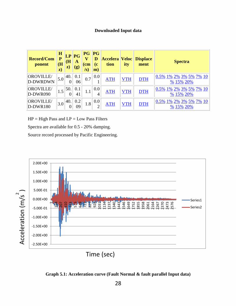
5.2.1 Input Data

After that the ground motion data was downloaded from PEER strong motion database.

The analysis are performed for 2 sets of ground motion records (FN and FP) for the “Oroville

1975/08/08 07:00” earthquake at 1543 DWR Garage station. The acceleration time history was

recorded for every 0.005 seconds.

27

Fig 5.2: PEER Strong Motion Database

P0117: Earthquake and Station Details

Oroville 1975/08/08 07:00

Magnitude: M ( 4.7 ) Ml ( 4.9 ) Ms ( )

Station: 1543 DWR Garage

Data Source: CIT

Distance (km):

Closest to fault rupture ( )

Hypocentral ( 6.5 )

Closest to surface projection of rupture ( )

Site conditions:

Geomatrix or CWB ( A )

USGS ( )

28

Downloaded Input data

Record/Com

ponent

H

P

(H

z)

LP

(H

z)

PG

A

(g)

PG

V

(cm

/s)

PG

D

(c

m)

Accelera

tion

Veloc

ity

Displace

ment Spectra

OROVILLE/

D-DWRDWN 5.0

40.

0

0.1

06 0.7

0.0

1 ATH VTH DTH

0.5% 1% 2% 3% 5% 7% 10

% 15% 20%

OROVILLE/

D-DWR090 1.5

50.

0

0.1

41 1.1

0.0

4 ATH VTH DTH

0.5% 1% 2% 3% 5% 7% 10

% 15% 20%

OROVILLE/

D-DWR180 3.0

40.

0

0.2

09 1.8

0.0

2 ATH VTH DTH

0.5% 1% 2% 3% 5% 7% 10

% 15% 20%

HP = High Pass and LP = Low Pass Filters

Spectra are available for 0.5 - 20% damping.

Source record processed by Pacific Engineering.

Graph 5.1: Acceleration curve (Fault Normal & fault parallel Input data)

-2.50E+00

-2.00E+00

-1.50E+00

-1.00E+00

-5.00E-01

0.00E+00

5.00E-01

1.00E+00

1.50E+00

2.00E+00

1

10

4

20

7

31

0

41

3

51

6

61

9

72

2

82

5

92

8

10

31

11

34

12

37

13

40

14

43

15

46

16

49

17

52

18

55

19

58

20

61

21

64

22

67

23

70

24

73

25

76

Series1

Series2

Acc

eler

atio

n (

m/s

2 )

Time (sec)

29

5.2.2 Output data:

5.2.2.1 Time History Analysis:

The effect of the downloaded input ground motion data has been investigated on the structure

(SDF system) using the dynamic time history analysis.

After performing the dynamic time history analysis we have got the output data for both fault

normal and fault parallel components of Far Fault ground motions , and also the curves for

(acceleration, velocity and displacement) versus time were obtained which are shown in the

following figures:

Graph 5.2: Acceleration curve (Fault Normal & fault parallel)

-2.5

-2

-1.5

-1

-0.5

0

0.5

1

1.5

2

1

10

8

21

5

32

2

42

9

53

6

64

3

75

0

85

7

96

4

10

71

11

78

12

85

13

92

14

99

16

06

17

13

18

20

19

27

20

34

21

41

22

48

23

55

24

62

25

69

Series1

Series3

Acc

eler

atio

n (

m/s

2 )

Time (sec)

30

Graph 5.3: Acceleration curve (Fault Normal)

Graph 5.4: Acceleration curve (Fault Parallel)

Time (sec)

Acc

eler

atio

n (

m/s

2 )

Time (sec)

31

Graph 5.5: Velocity Curve (Fault Normal & Fault Parallel)

Graph 5.6: Velocity Curve (Fault Normal)

-0.02

-0.015

-0.01

-0.005

0

0.005

0.01

0.015

0.02

1

10

4

20

7

31

0

41

3

51

6

61

9

72

2

82

5

92

8

10

31

11

34

12

37

13

40

14

43

15

46

16

49

17

52

18

55

19

58

20

61

21

64

22

67

23

70

24

73

25

76

Series1

Series2

Time (sec)

Vel

oci

ty (

m/s

) V

elo

city

(m

/s)

Time (sec)

32

Graph 5.7: Velocity curve (Fault parallel)

Graph 5.8: Displacement Curve (Fault Normal & Fault Parallel)

-0.0004

-0.0003

-0.0002

-0.0001

0

0.0001

0.0002

0.0003

0.0004

19

71

93

28

93

85

48

15

77

67

37

69

86

59

61

10

57

11

53

12

49

13

45

14

41

15

37

16

33

17

29

18

25

19

21

20

17

21

13

22

09

23

05

24

01

24

97

25

93

Series1

Series2

Time (sec)

Vel

oci

ty (

m/s

) D

isp

lace

men

t (m

)

Time (sec)

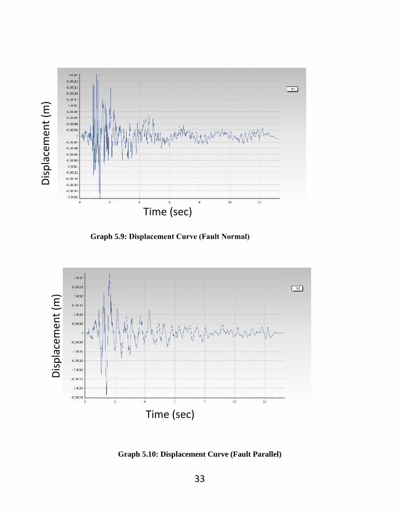
33

Graph 5.10: Displacement Curve (Fault Parallel)

Graph 5.9: Displacement Curve (Fault Normal)

Dis

pla

cem

ent

(m)

Time (sec)

Time (sec)

Dis

pla

cem

ent

(m)

34

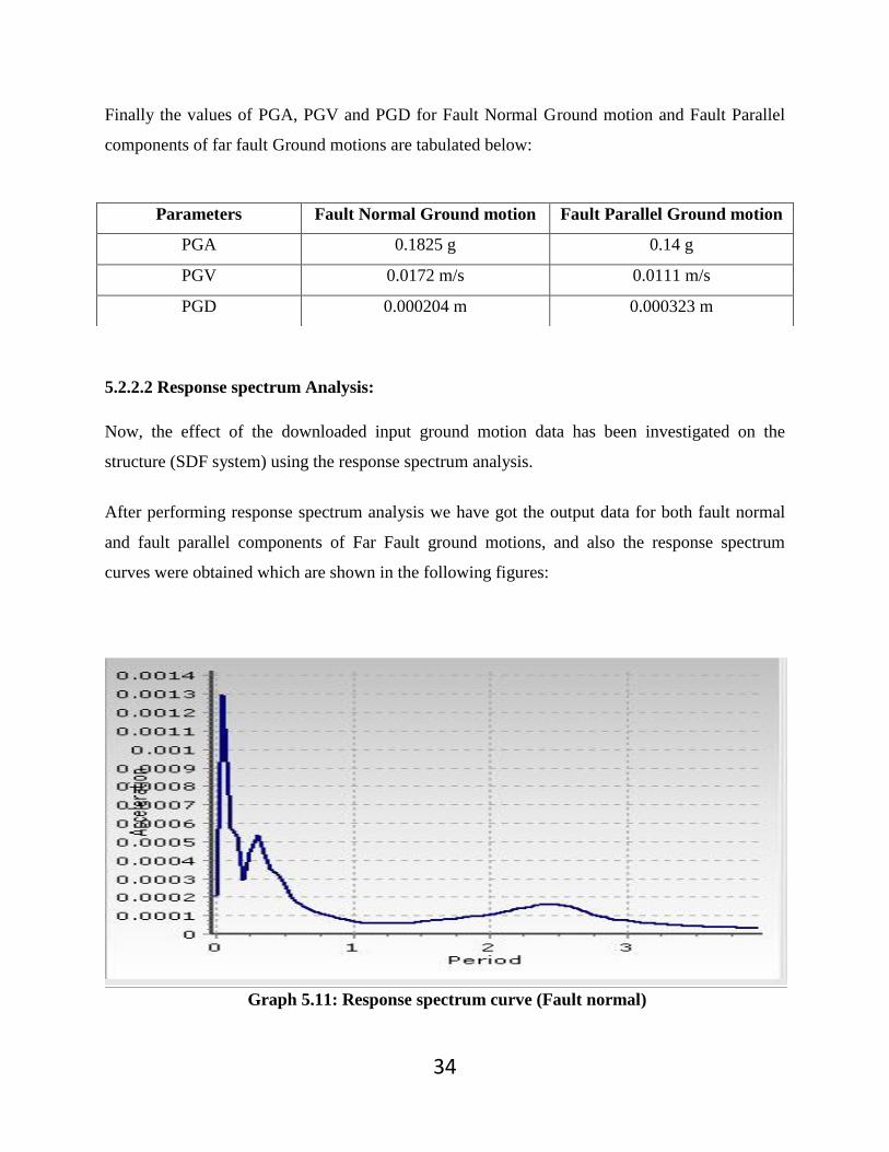
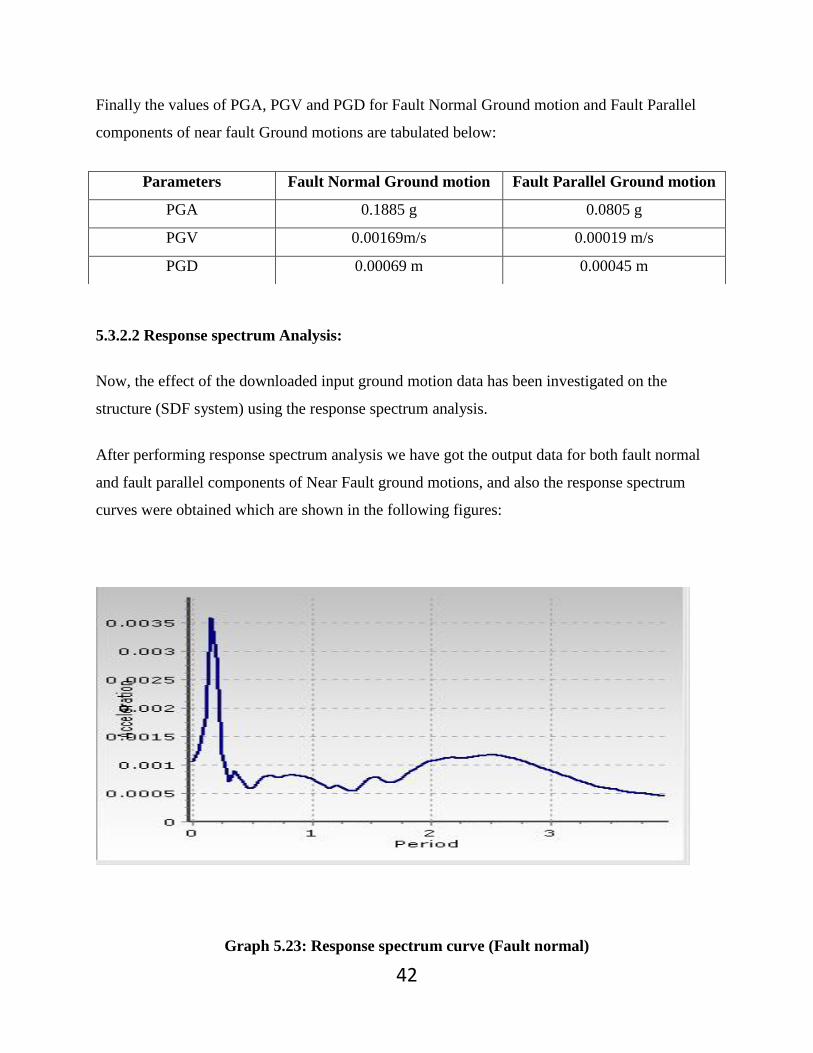
Finally the values of PGA, PGV and PGD for Fault Normal Ground motion and Fault Parallel

components of far fault Ground motions are tabulated below:

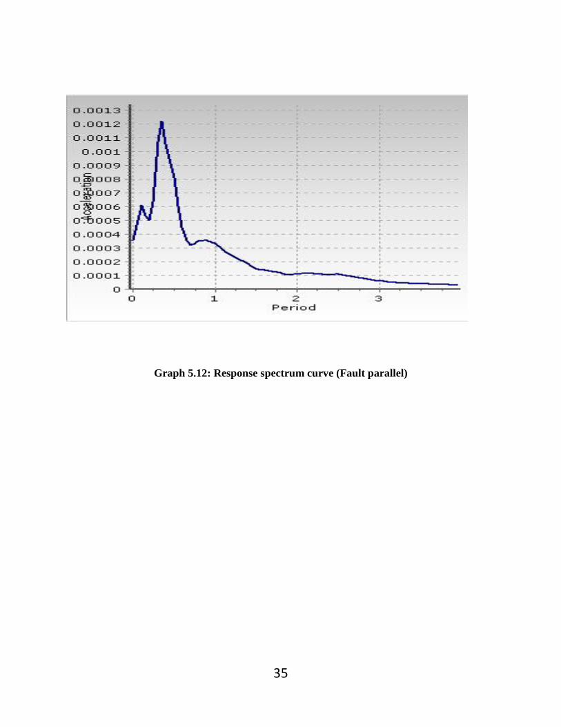
5.2.2.2 Response spectrum Analysis:

Now, the effect of the downloaded input ground motion data has been investigated on the

structure (SDF system) using the response spectrum analysis.

After performing response spectrum analysis we have got the output data for both fault normal

and fault parallel components of Far Fault ground motions, and also the response spectrum

curves were obtained which are shown in the following figures:

Graph 5.11: Response spectrum curve (Fault normal)

Parameters Fault Normal Ground motion Fault Parallel Ground motion

PGA 0.1825 g 0.14 g

PGV 0.0172 m/s 0.0111 m/s

PGD 0.000204 m 0.000323 m

35

Graph 5.12: Response spectrum curve (Fault parallel)

36

5.3 Near Fault Earthquake:

5.3.1 Input data:

The analysis are performed for 2 sets of ground motion records (FN and FP) for the OROVILLE

08/08/75 07:00, JOHNSON RANCH, (CDMG STATION 1493). The acceleration time history

was recorded for every 0.005 seconds.

Graph 5.13: Acceleration curve (Fault Normal & fault parallel Input data)

5.3.2 Output data:

5.3.2.1Time History Analysis:

The effect of the downloaded input ground motion data has been investigated on the structure

(SDF system) using the dynamic time history analysis.

-2.50E+00

-2.00E+00

-1.50E+00

-1.00E+00

-5.00E-01

0.00E+00

5.00E-01

1.00E+00

1.50E+00

2.00E+00

2.50E+00

1

10

5

20

9

31

3

41

7

52

1

62

5

72

9

83

3

93

7

10

41

11

45

12

49

13

53

14

57

15

61

16

65

17

69

18

73

19

77

20

81

21

85

22

89

23

93

24

97

Series1

Series2

Acc

eler

atio

n (

m/s

2 )

Time (sec)

37

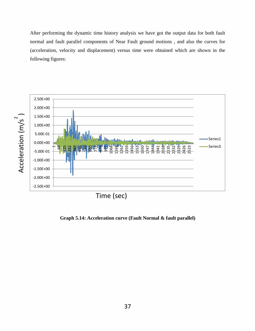
After performing the dynamic time history analysis we have got the output data for both fault

normal and fault parallel components of Near Fault ground motions , and also the curves for

(acceleration, velocity and displacement) versus time were obtained which are shown in the

following figures:

Graph 5.14: Acceleration curve (Fault Normal & fault parallel)

-2.50E+00

-2.00E+00

-1.50E+00

-1.00E+00

-5.00E-01

0.00E+00

5.00E-01

1.00E+00

1.50E+00

2.00E+00

2.50E+00

1

98

19

5

29

2

38

9

48

6

58

3

68

0

77

7

87

4

97

1

10

68

11

65

12

62

13

59

14

56

15

53

16

50

17

47

18

44

19

41

20

38

21

35

22

32

23

29

24

26

25

23

Series1

Series3

Acc

eler

atio

n (

m/s

2 )

Time (sec)

38

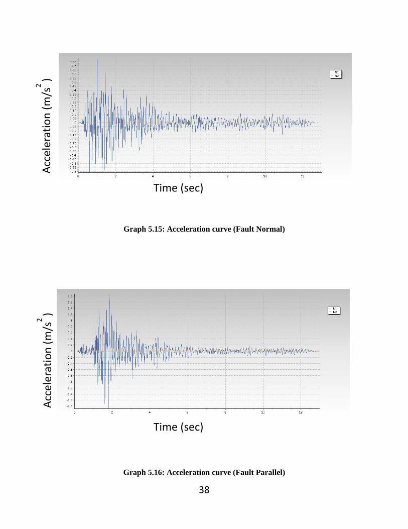
Graph 5.15: Acceleration curve (Fault Normal)

Graph 5.16: Acceleration curve (Fault Parallel)

Acc

eler

atio

n (

m/s

2 )

Acc

eler

atio

n (

m/s

2 )

Time (sec)

Time (sec)

39

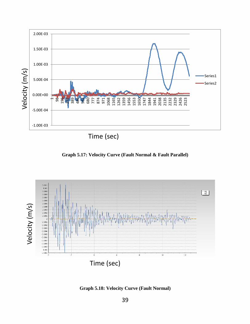
Graph 5.17: Velocity Curve (Fault Normal & Fault Parallel)

Graph 5.18: Velocity Curve (Fault Normal)

-1.00E-03

-5.00E-04

0.00E+00

5.00E-04

1.00E-03

1.50E-03

2.00E-03

1

98

19

5

29

2

38

9

48

6

58

3

68

0

77

7

87

4

97

1

10

68

11

65

12

62

13

59

14

56

15

53

16

50

17

47

18

44

19

41

20

38

21

35

22

32

23

29

24

26

25

23

Series1

Series2

Vel

oci

ty (

m/s

)

Time (sec)

Vel

oci

ty (

m/s

)

Time (sec)

40

Graph 5.19: Velocity curve (Fault parallel)

Graph 5.20: Displacement Curve (Fault Normal & Fault Parallel)

-1.20E-03

-1.00E-03

-8.00E-04

-6.00E-04

-4.00E-04

-2.00E-04

0.00E+00

2.00E-04

4.00E-04

6.00E-04

8.00E-04

1

98

19

5

29

2

38

9

48

6

58

3

68

0

77

7

87

4

97

1

10

68

11

65

12

62

13

59

14

56

15

53

16

50

17

47

18

44

19

41

20

38

21

35

22

32

23

29

24

26

25

23 Series2

Series3

Vel

oci

ty (

m/s

)

Time (sec)

Dis

pla

cem

ent

(m)

Time (sec)

41

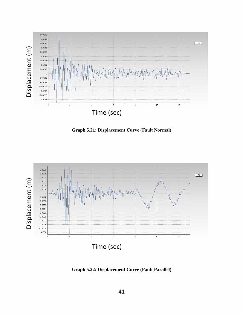
Graph 5.21: Displacement Curve (Fault Normal)

Graph 5.22: Displacement Curve (Fault Parallel)

Dis

pla

cem

ent

(m)

Dis

pla

cem

ent

(m)

Time (sec)

Time (sec)

42

Finally the values of PGA, PGV and PGD for Fault Normal Ground motion and Fault Parallel

components of near fault Ground motions are tabulated below:

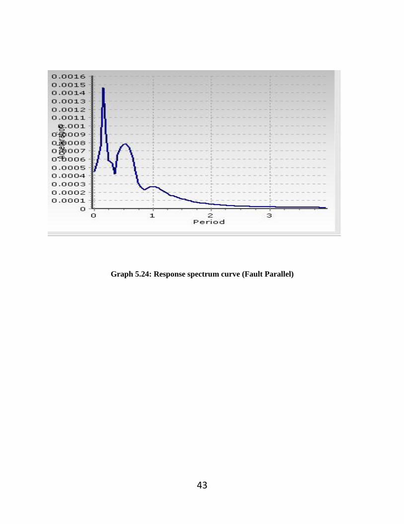
5.3.2.2 Response spectrum Analysis:

Now, the effect of the downloaded input ground motion data has been investigated on the

structure (SDF system) using the response spectrum analysis.

After performing response spectrum analysis we have got the output data for both fault normal

and fault parallel components of Near Fault ground motions, and also the response spectrum

curves were obtained which are shown in the following figures:

Graph 5.23: Response spectrum curve (Fault normal)

Parameters Fault Normal Ground motion Fault Parallel Ground motion

PGA 0.1885 g 0.0805 g

PGV 0.00169m/s 0.00019 m/s

PGD 0.00069 m 0.00045 m

43

Graph 5.24: Response spectrum curve (Fault Parallel)

44

CHAPTER 6

SUMMARY AND

CONCLUSION

45

6.1 SUMMARY:

In the current study the performance of a structure in a single degree of freedom system is

investigated under different ground motions such as Fault normal and Fault parallel component

of the ground motion by dynamic time history analysis method and the analysis is done in the

SEISMOSTRUCT software developed by the SEISMOSOFT Company.

The Acceleration, Velocity and displacement curves have been drawn for both Fault Normal and

Fault Parallel component of Far Fault and Near Fault ground motion. The values of acceleration,

velocity, displacement have been found in every 0.005 seconds, also the values of Peak Ground

Acceleration, Peak Ground Velocity and Peak Ground Displacement has been determined for

both components.

Finally the response spectrum curves have been drawn for each kind of earthquake ground

motions.

6.2 CONCLUSION:

The values of Peak Ground Acceleration, Peak Ground Velocity and Peak Ground

Displacement obtained for fault normal component are higher than that of fault parallel

component.

The frequencies for fault normal component are higher than that of the fault parallel.

The values of Peak Ground Acceleration, Peak Ground Velocity and Peak Ground

Displacement of Fault Normal and Fault parallel components don’t differ much for Far

Fault earthquake ground motions, but they differ much for Near Fault Earthquake ground

motions.

The response spectrum curves are different for each kind of earthquake ground motions,

hence it means that the structure have different responses to each kind of earthquake

ground motions.

46

CHAPTER 7

REFERENCES

47

7.1 REFERENCES:

1. Mario Paz,1979, “Structural Dynamics” 2nd

Edition, CBS Publishers and Distributors

2. www.sciencedirect.com (8th

September 2014)

3. IS1893-2002, Indian Standard CRITERIA FOR EARTHQUAKE RESISTANTDESIGN

OF STRUCTURE, Bureau of Indian Standards, Fifth revision

4. En.wikipedia.org/wiki/Fault_(geology) (5th

September 2014)

5. www.seismosoft.com (1st September 2014)

6. IS 456 (2000) “Indian Standard for Plain and Reinforced Concrete” Code of Practice,

Bureau of Indian Standards, New Delhi, 2000

7. S. Yaghmaei-Sabegh and N. Jalali-Milani, 2012 “Pounding force response spectrum for

near-field and far-field earthquakes”

8. Kalkan, E., and Kwong, N.S., 2012, “Evaluation of fault-normal/fault-parallel directions

rotated ground motions for response history analysis of an instrumented six-story

building”

9. Douglas Dreger, Gabriel Hurtado, Anil K. Chopra, Shawn Larsen, 2007 “Near fault

seismic ground motion”

10. IS 875 (part1), Dead loads, unit weights of building material and stored and stored

material (second revision), New Delhi 110002: Bureau of Indian Standards, 1987.

11. IS 875 (part2) Imposed loads (second revision), New Delhi 110002: Bureau of Indian

Standards, 1987.

12. J.C. Reyes and E. Kalkan, 2012, “Relevance of Fault-Normal/Parallel and Maximum

Direction Rotated Ground Motions on Nonlinear Behavior of Multi-Story Buildings”

13. Chan, C.M. and Zou, X.K. (2004) Elastic and inelastic drift performance optimization for

reinforced concrete buildings under earthquake loads. Earthquake Engineering and

Structural Dynamics 33,929–950

14. EC8, Design of structures for earthquake resistance, Part 1: General rules, seismic actions

and rules for buildings. European committee for standardization, Brussels, 2002

15. Agarwal A. (2012): Seismic Evaluation of Institute Building, Bachelor of Technology

Thesis, National Institute of Technology Rourkela

48

16. Applied Technology Council (ATC), Seismic Evaluation and Retrofit of Concrete

Buildings. ATC-40, Redwood City, CA, 1996.

17. M. L. Gambhir, Fundamentals of Reinforced Concrete Design, New Delhi- 110001: PHI

Learning Private Limited, 2010.

18. Manish Shrikhande and Pankaj Agarwal “Earthquake Resistant Design of Structures” 1st

Edition.

19. R. Clough, and J. Penzien, Dynamics of Structures, McGraw-Hill, New York. 1993