response of electrical transmission line conductors
TRANSCRIPT
RESPONSE OF ELECTRICAL TRANSMISSION LINE CONDUCTORS
TO EXTREi^E WIND USING FIELD DATA
by
RADHAKRISHNA R. KADABA, B.E., M.E.
A DISSERTATION
IN
CIVIL ENGINEERING
Submitted to the Graduate Faculty of Texas Tech University in
Partial Fulfillment of the Requirements for
the Degree of
DOCTOR OF PHILOSOPHY
Approved
May, 1988
ACKNOWLEDGEMENTS
I would like to express my special thanks and sincere
gratitude to the chairman of my committee. Dr. Kishor C.
Mehta, for his guidance, everlasting inspiration, constant
encouragement and patience in teaching me throughout my
graduate study program. I am also grateful to Drs. Eric L.
Blair, H. Scott Norville, William Pennington Vann, and Y.C.
Das, the members of my advisory committee, for their helpful
review and constructive criticism of this dissertation.
The research was accomplished under the financial
support of the Bonneville Power Administration (BPA) and the
Institute for Disaster Research (IDR) at Texas Tech
University. Support of these organizations is appreciated.
Special thanks are extended to Mr. Leon Kempner, Jr. for his
assistance in providing the field data details of the BPA
project and encouragement. Also, I would like to express my
deep appreciation to the Chairman of the Civil Engineering
Department, Dr. Ernst W. Kiesling, for his encouragement and
support during the course of my graduate study.
I shall ever remain indebted to my sister Vijaya
Bhanuprakash, brother Udaya Kumar, sister-in-law Latha
Ananth, and my other family members for their kind blessings
11

and the moral support during my stay away from home.
Special thanks are given for the assistance and friendship
provided by my colleagues Suresh Jonnagadla, Marc Levitan,
Saranga Kidambi and Pankaja Kidambi.
I must acknowledge with deep appreciation and
encouragement of my brother, Sri. Anantharamu, who instilled
in me the value of education and stood by my side giving all
the moral support he could and most of all his kind prayers
and love.
Finally, I would like to express 'Thanks' to my
parents, to whom I dedicate this dissertation.
Ill
11
vi
CONTENTS
ACKNOWLEDGEMENTS
ABSTRACT
LIST OF TABLES viii
LIST OF FIGURES x
CHAPTER
I. INTRODUCTION 1
Objectives ' 5
Contents of the Dissertation 6
II. STATE OF KNOWLEDGE 7
Response 8 Mean Response 10 Fluctuating Response 12
Aerodynamic Admittance Function 16 Mechanical Admittance Function 19
Peak Factor 20 Wind Characteristics 24
Mean Wind Speed 24 Mean Wind Profile 25 Turbulence Characteristics 28
Turbulence Intensity 30 Gust Spectrum 31
Davenport Analytical Model 34 Conductor Damping Ratio 37 Conductor Fundamental Frequency 38
III. FIELD DATA 39
Description of Test Site 41 Instrumentation 43 Data Accjuisition 47 Recording Procedure 48 Description of Recordings 50
IV
IV. FIELD DATA ANALYSIS 52
Validity of Wind Data 53 Power-Law Exponent for Wind Profile 60 Turbulence Intensity 65 Kaimal's Gust Spectrum Constants 68 Validity of Conductor Response Data 74 Effective Conductor Force Coefficient 80 Response Spectrum 85
V. COMPARISON AND REFINEMENT OF THE ANALYTICAL MODEL 90
Comparison of Analytically Predicted Mean Scjuare Response With Field Measured Values 91
Field Measured Mean Square Response 92 Analytical Model Predicted Mean Scjuare
Response 94 Refinement of the Analytical Model 104
Background Response 104 Determining the JAF Coefficients 108
Resonant Response 115 Determining the Aerodynamic Damping Ratio 115
Resonant Response with Suggested Damping Ratio 123
Peak Factors 127 Probabilistic Peak Factors from Field
Data 130
VI. CONCLUSIONS 134
REFERENCES 138
ABSTRACT
Conductors are long, slender, flexible, and wind
sensitive structures. In most cases of transmission lines,
60-80% of wind loads coming to the support structures are
transferred from conductors. Thus, assessment of conductor
response due to extreme wind is an important part of the
overall prediction of wind loads on transmission structures,
Extreme winds not only contain high wind speeds but also
randomly fluctuating gusts. These gusts cause fluctuating
dynamic responses of conductors. Since the responses
fluctuate randomly, they need to be assessed in
probabilistic terms.
An analytical model for estimating dynamic response of
transmission line structures to wind loads is developed by
Davenport. The model can be verified using field data to
determine its effectiveness. Bonneville Power
Administration (BPA) has conducted experimental studies in
the field at the Moro site to collect wind and electric
transmission structure response data. During 1981-1982 BPA
collected 23 separate 12-minute duration records that
included wind speed, wind direction and conductor response
data. The conductor response records include load cell.
VI
transverse swing angle, and longitudinal swing angle
recordings.
The BPA data of wind and conductor response are
analyzed in detail to gain as much information as possible.
The analysis of wind data include determination of wind
characteristics of mean wind profile, turbulence
intensities, and gust spectra. The conductor response in
terms of peak responses, effective force coefficients, peak
factors, and response spectra are obtained. The response
spectra are further analyzed to obtain contributions of
background response and resonant response. Comparison of
the analytical model with field data reveals that the model
underestimated background response and overestimated
resonant response.
Results of these data analyses are used to improve the
analytical model to predict conductor response in extreme
wind. The significant improvement includes determination of
peak factors from upcrossing rates, refinement in the
expression for background response and determination of
conductor aerodynamic damping ratios from field data.
VI1
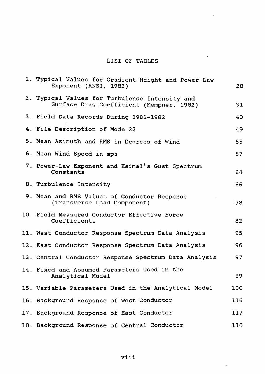
LIST OF TABLES
1. Typical Values for Gradient Height and Power-Law Exponent (ANSI, 1982) 28
2. Typical Values for Turbulence Intensity and
Surface Drag Coefficient (Kempner, 1982) 31
3. Field Data Records During 1981-1982 40
4. File Description of Mode 22 49
5. Mean Azimuth and RMS in Degrees of Wind 55
6. Mean Wind Speed in mps 57
7. Power-Law Exponent and Kaimal's Gust Spectrum
Constants 64
8. Turbulence Intensity 66
9. Mean and RMS Values of Conductor Response (Transverse Load Component) 78
10. Field Measured Conductor Effective Force
Coefficients 82
11. West Conductor Response Spectrum Data Analysis 95
12. East Conductor Response Spectrum Data Analysis 96
13. Central Conductor Response Spectrum Data Analysis 97
14. Fixed and Assumed Parameters Used in the
Analytical Model 99
15. Variable Parameters Used in the Analytical Model 100
16. Background Response of West Conductor 116
17. Background Response of East Conductor 117
18. Background Response of Central Conductor 118
Vlll
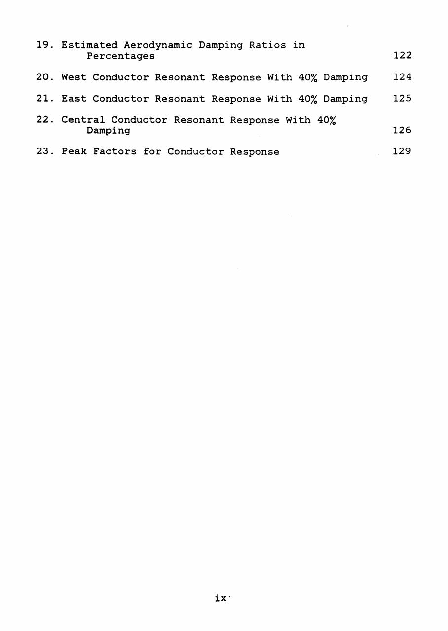
19. Estimated Aerodynamic Damping Ratios in
Percentages 122
20. West Conductor Resonant Response With 40% Damping 124
21. East Conductor Resonant Response With 40% Damping 125
22. Central Conductor Resonant Response With 40% Damping 126
23. Peak Factors for Conductor Response 129
IX'
LIST OF FIGURES
1. Fluctuations of Wind Speed 3
2. Fluctuations of Conductor Response 3
3. Conductor Force Coefficients Based on Wind Tunnel
and Full-Scale Tests (Davenport, 1980) 13
4. Elements of Response Spectrum Analysis 15
5. Example of a Random Variable Showing Upcrossings of a Given Threshold 22
6. Idealization of Gust Spectrum Plot Over an
Extended Range (Davenport, 1972) 26
7. Topography of Site and Orientation of Power Lines 42
8. Schematic of Tower 16/4 44
9. Elevation Along the Test Line (Vertical Scale Exaggerated) 45
10. Time History Plot of Wind Speed for Record NOl at 34.7 m on Tower 16/4 59
11. Mean Wind Speed and Direction Recorded at 34.7 m
on Tower 16/4 of 23 Records 61
12. Power-Law Plot for Record N15 63
13. Gust Spectrum Plot for Record NOl Recorded at 34.7 m on Tower 16/4 70
14. Time History Plot of West Conductor Response for Record NOl 76
15. Response Spectrum Plot for West Conductor Response for Record NOl 86
16. West Conductor Response Spectrum Plot for Record NOl 93
X
17. Analytical Model Background Response Versus Field Measured Background Response 102
18. Analytical Model Resonant Response Versus Field Measured Resonant Response 103
19. Frequency Transfer Function of West Conductor Response for Record NOl 110
20. West Conductor JAF Coefficients Contour Plot for
Record N15 112
21. Joint Acceptance Function Plot 114
22. Refined Model Background Response Versus Field Measured Values 119
23. Analytical Model Resonant Response With 40% Damping Versus Field Measured Values 128
24. Cumulative Probability Distribution of Upcrossings for Conductor Response 133
XI
CHAPTER I
INTRODUCTION
Electrical transmission line systems are engineered
structures that traverse over all types of terrain. Wind
loading is an important factor in the design of these
transmission line systems, consisting of towers, conductors,
and ground wires. Transmission line conductors are long,
flexible, and wind sensitive structures. Probably no other
structure has as much of its mass in highly flexible form,
and so continuously exposed to the forces of wind, as do
transmission line conductors. The loads due to the effect
of wind acting on the conductors, which in turn, transmit
loads to the supporting tower, are more than the loads due
to the wind acting directly on the tower itself. Wind loads
on conductors with spans of around 300 m account for 60 to
80% of the total wind load effect on the support tower
structure. Accurate and reliable prediction of wind loads
that are transferred from conductors to the towers are
desirable to produce an economical and safe design of
support tower structures.
Transmission line tower structures are usually designed
for five different types of loads (Kempner, 1985): (1)
extreme wind, (2) wind on ice, (3) National Electric Safety
Code (NESC, 1984), (4) broken conductor, and (5)
construction loading. Records show that more than 50% of
tower structure failures are due to extreme winds. Under
these conditions, any improvement in the understanding of
conductor behavior under extreme winds which leads to better
definition of loads and better accompanying design of the
tower structure is desirable.
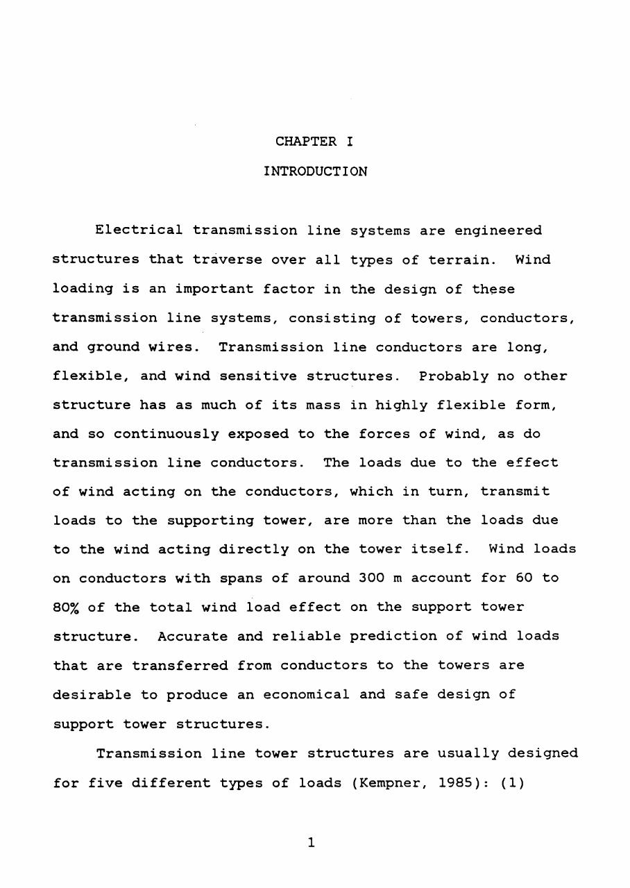
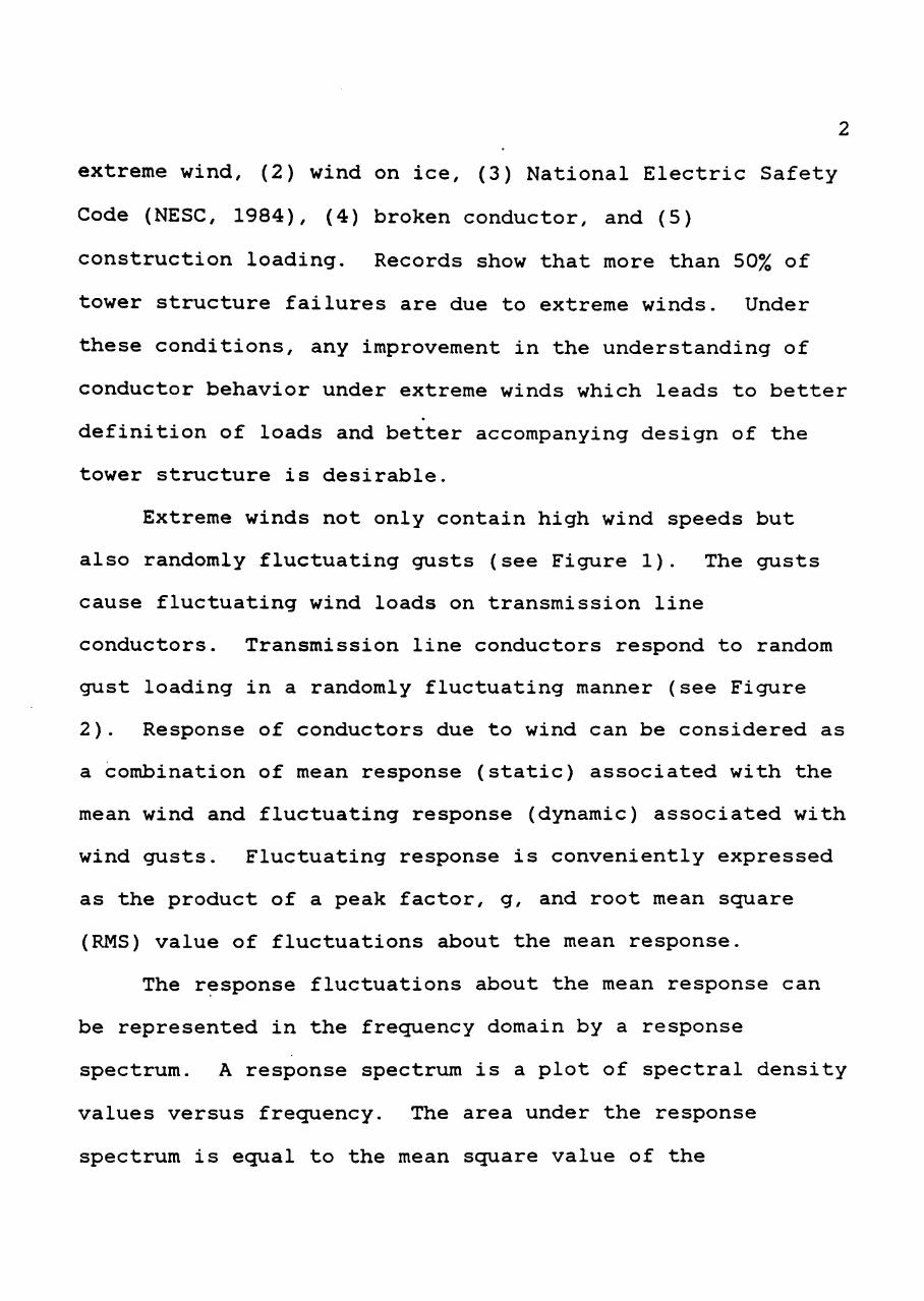
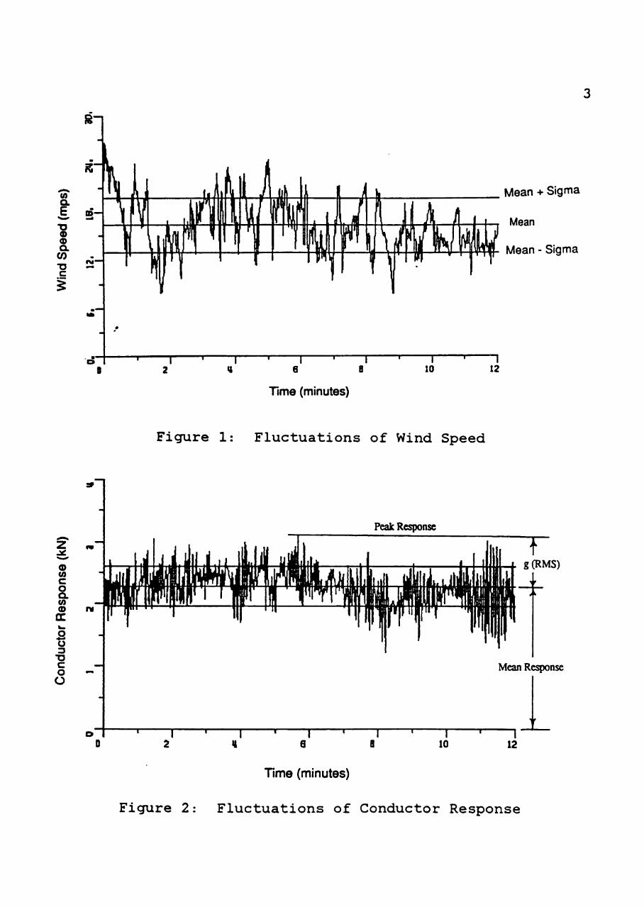
Extreme winds not only contain high wind speeds but
also randomly fluctuating gusts (see Figure 1). The gusts
cause fluctuating wind loads on transmission line
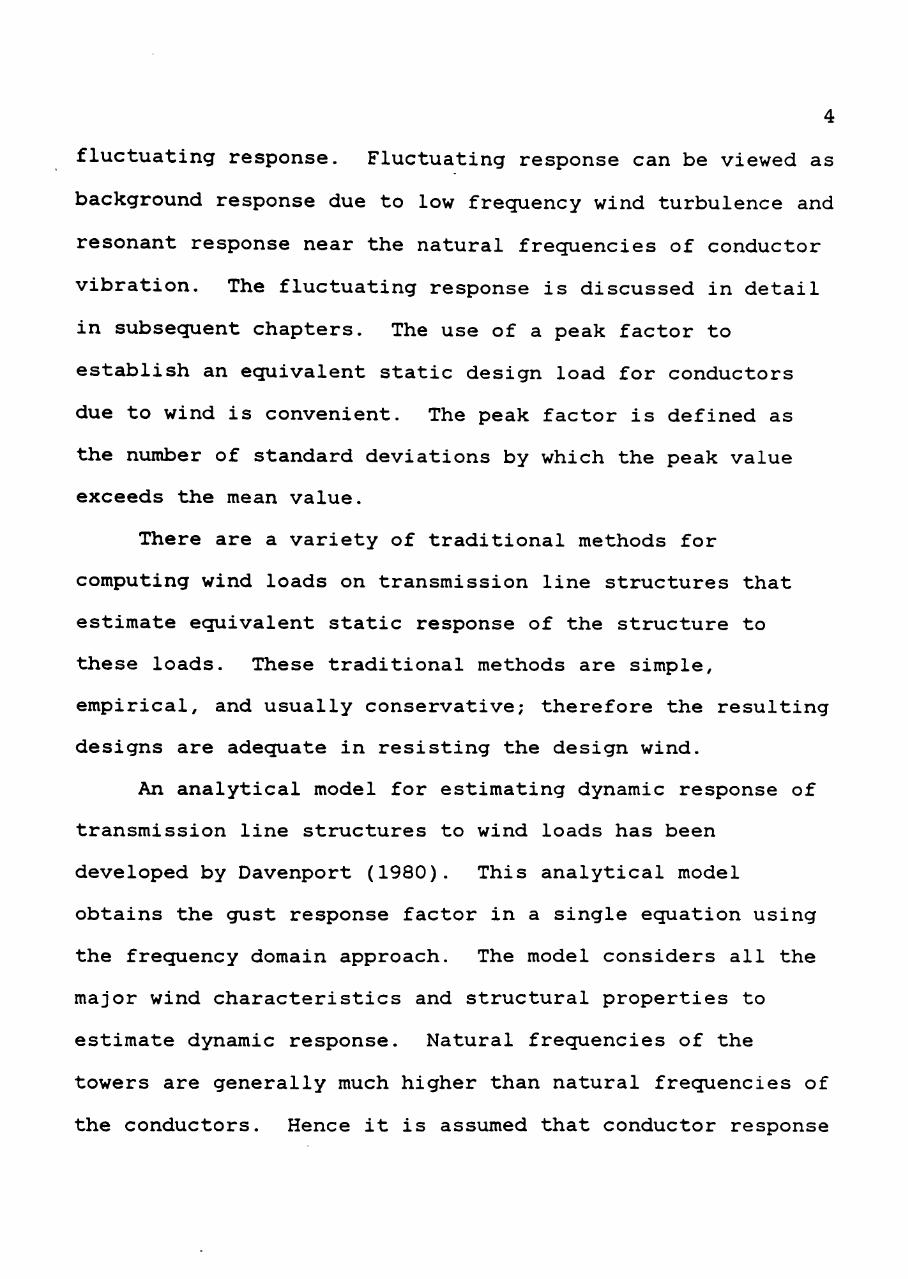
conductors. Transmission line conductors respond to random
gust loading in a randomly fluctuating manner (see Figure
2). Response of conductors due to wind can be considered as
a combination of mean response (static) associated with the
mean wind and fluctuating response (dynamic) associated with
wind gusts. Fluctuating response is conveniently expressed
as the product of a peak factor, g, and root mean scjuare
(RMS) value of fluctuations about the mean response.
The response fluctuations about the mean response can
be represented in the frecjuency domain by a response
spectrum. A response spectrum is a plot of spectral density
values versus frecjuency. The area under the response
spectrum is ecjual to the mean square value of the
a
•a a> o Q.
en c
Mean + Sigma
Mean
Mean - Sigma
Time (minutes)
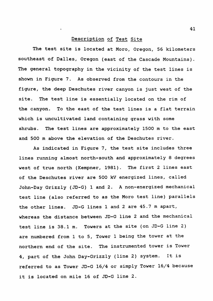
Figure 1: Fluctuations of Wind Speed
o c o a. a>
o t5 •a c o O
Time (minutes)
Figure 2: Fluctuations of Conductor Response
fluctuating response. Fluctuating response can be viewed as
background response due to low frequency wind turbulence and
resonant response near the natural frecjuencies of conductor
vibration. The fluctuating response is discussed in detail
in subsecjuent chapters. The use of a peak factor to
establish an equivalent static design load for conductors
due to wind is convenient. The peak factor is defined as
the number of standard deviations by which the peak value
exceeds the mean value.
There are a variety of traditional methods for
computing wind loads on transmission line structures that
estimate ecjuivalent static response of the structure to
these loads. These traditional methods are simple,
empirical, and usually conservative; therefore the resulting
designs are adecjuate in resisting the design wind.
An analytical model for estimating dynamic response of
transmission line structures to wind loads has been
developed by Davenport (1980). This analytical model
obtains the gust response factor in a single equation using
the frecjuency domain approach. The model considers all the
major wind characteristics and structural properties to
estimate dynamic response. Natural frecjuencies of the
towers are generally much higher than natural frecjuencies of
the conductors. Hence it is assumed that conductor response

is not influenced by the motion of the supporting tower
structure. With the above assumption, the response due to
wind on the conductor and on the tower structure can be
analyzed separately.
Wind tunnel experiments and full-scale field tests have
been conducted on transmission line structures. Because of
their slenderness and flexibility full-scale tests are
especially significant to assess dynamic response of these
structures. Full-scale tests are of great value to compare
and refine the analytical model. The most comprehensive
source of full-scale data is the experiments conducted on
John Day-Grizzly transmission line 2 located in northern
Oregon. These field data, collected by the Bonneville Power
Administration, are used in this study. The data include
simultaneous recordings of wind and transmission line
response during extreme winds. Analysis of field data of
wind and transmission line conductor response can assist in
substantiating and improving the analytical model.
Objectives
The general objective of this research is to determine
the dynamic response of conductors due to extreme wind using
field data. The Specific objectives are: (1) to assess
wind parameters from the field data, (2) to develop
probabilistic peak factors for conductor response using
upcrossing rates, (3) to determine the aerodynamic damping
and the joint acceptance function for conductors from the
field response data, and (4) to compare dynamic response of
conductors measured in the field with a refined analytical
model.
Content of the Dissertation
A brief description of the contents of this
dissertation is given here. The next chapter contains an
overview of the state of knowledge concerning wind
characteristics, and details of the analytical model to be
used to predict dynamic response of conductors. A
description of the measurements, site characteristics, and
instrumentation for the field data is given in Chapter III.
Analyses of wind and conductor response field data are
described in Chapter IV. Comparisons of field measured
conductor response data with responses calculated using the
analytical model are part of Chapter V. Determination of
probabilistic peak factors for conductor response using the
upcrossing rate principle, refinement of the background
response expression, and determination of conductor
aerodynamic damping from the field response data are also
presented in this chapter. Conclusions reached in this
study are presented in Chapter VI.
CHAPTER II
STATE OF KNOWLEDGE
Wind loads on transmission line conductors depend on
wind characteristics and on interaction phenomena of the
wind with conductors. Wind speed fluctuates randomly; it
can be considered to consist of mean and fluctuating (or
gust) components. A knowledge of both the mean wind speed
and the random fluctuations are recjuired to evaluate wind
loading. In addition, structural properties (natural
frecjuencies, damping, size, shape,..etc) play an important
role in prediction of response of the conductors in extreme
winds.
The difficulty of proper simulation of the natural wind
characteristics and scaling of transmission line structures
in wind tunnels leads researchers to depend on full-scale
experiments. There have been only a few full-scale
experiments for wind loads on transmission line structures.
Field measurement programs have been conducted in the United
States, Canada, Europe, and Japan to monitor the wind
response of transmission line systems. A review of each of
the field test programs is given in a report by GAI
consultants (1981). These field tests measured wind and
8
response data for a specific design objective such as
determination of the span factor or the gust response
factor. Detailed analyses of field data are not reported in
the open literature. Bonneville Power Administration (BPA)
has conducted field experiments on transmission line
structures since 1976. Results of analysis of BPA data are
available in several reports and papers (Kempner and
Laursen, 1977, 1979, 1981; Kempner and Thorkildson, 1982;
Ferraro, 1983; Norville, 1985). These reports and the
present study indicate that conductor response to extreme
winds is governed by wind turbulence characteristics,
aerodynamic characteristics of wind structure interaction
and structural dynamics of the conductors. The wind and
conductor response data collected by BPA during 1981-1982
are used in the present study. The literature on wind,
aerodynamics, and structural dynamics is very extensive.
Only the items that are obtainable through analysis of field
data and are pertinent to this study are discussed in this
section.
Response
The design of a transmission line tower structure is
generally based on the peak transverse load component of the
conductors when subjected to extreme winds. The transverse
load component transferred to the tower is the direct result
of the transverse response of the conductor. The the
transverse load component is considered as conductor
response in the present study. The prediction of this peak
response value, rather than a mean response value, is needed
for design purposes. Peak response is predicted by the
summation of mean and fluctuating responses. For a time
period, T, the peak response can be estimated by
ft = R + g aj (2.1)
where ft = peak response,
R = mean response,
a„ = root mean scjuare (RMS) of the fluctuating
response about the mean response, and
g = statistical peak factor.
In ecjuation 2.1, the mean response is based on the mean
wind speed. The fluctuating response is a product of peak
factor and RMS value of response. The dimensionless peak
factor, g, is probabilistic because of the random nature of
the fluctuating response. The peak factor is determined
from the probability of the upcrossing rate or,
ecjuivalently, a specified number of occurrences in a given
interval of time. The RMS of the fluctuating response

10
depends on wind characteristics such as the turbulence
intensity and structural characteristics such as the
damping, frecjuency, shape,., etc.
Mean Response
The mean response of conductors is obtained from the
mean wind pressure acting at the effective height of the
conductors. The effective height of the conductor is
considered as the average height of the conductor above the
ground level. The ecjuation for mean wind pressure is
1 -2 P = y P V C^ (2.2)
where P = mean wind pressure,
p = mass density of air, 1.226 kg m' , at 60 F,
at sea level,
V = mean wind speed at the effective conductor
height, and
C^ = conductor force coefficient.
The mean response of conductors, R, can now be expressed as:
R = P L d (2.3)
where L = effective conductor span, and
d = conductor diameter.
11
The mean response of a conductor depends on the mean
wind speed and the aerodynamic relationship in terms of
conductor force coefficient. The force coefficient converts
the stagnation pressure term (- pV ) in ecjuation 2.2 to a
transverse force on the conductor. In most cases, the force
coefficient is determined from wind tunnel tests and, in
general, it is a function of Reynolds Number, the angle of
incidence of the wind, and the shape and roughness of the
conductor. Published results of wind tunnel measurements
show wide variability in force coefficient values, because
of difficulty in simulation of Reynolds Number and varying
tests conditions (Potter, 1981).
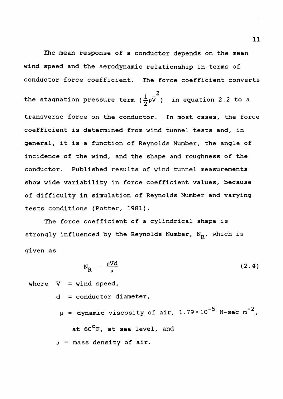
The force coefficient of a cylindrical shape is
strongly influenced by the Reynolds Number, Nj^, which is
given as
Np = -B^ (2.4)
R \x
where V = wind speed,
d = conductor diameter, -5 -2
1 = dynamic viscosity of air, 1.79x10 N-sec m
at 60°F, at sea level, and
p = mass density of air.
12
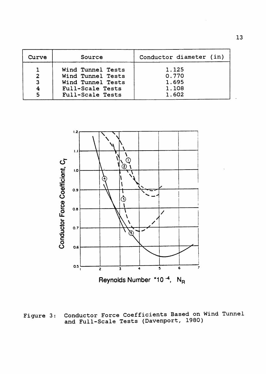
A plot of force coefficient versus Reynolds Number is
shown in Figure 3. The region of the curve where the force
coefficient decreases sharply with Reynolds Number is called
the critical flow range. This decrease in force coefficient
is related to the transition from laminar flow to turbulent
flow. For a typical conductor diameter and design wind
speed, the Reynolds Number is usually above the critical
4 range (N„ > 5 x 10 ) . A constant value for the conductor
force coefficient is usually given in transmission line
design recommendations (ASCE, 1984). As indicated in Figure
3, full-scale measurements tend to give lower force
coefficient values than the wind tunnel experiments. These
discrepancies are not yet resolved in the published
literature. Additional data on force coefficients from
field measurements are desirable.
Fluctuating Response
Conductor response to fluctuating wind depends upon the
dynamic characteristics of the conductor as well as
turbulence in the wind. To determine the response of a
conductor subjected to fluctuating wind, frecjuency domain
methods are usually used. Frecjuency domain methods are
popular for computation because they are cost effective and
efficient. In frecjuency domain analysis, fluctuations in
13
Curve
1 2 3 4 5
Source
Wind Tunnel Tests Wind Tunnel Tests Wind Tunnel Tests Full-Scale Tests Full-Scale Tests
Conductor diameter (in)
1.125 0.770 1.695 1.108 1.602
1.2
o
o o
o o P
B o •o c o O
to
0.9
0.8
0.7
0.6
0.5
>
\
w
\ \
\
(D\
1 (1) \ \
\ \ V
^^-\ ^ —
/ /
^
^
/
1 1
i
Reynolds Number *10•^ NR
Figure 3: Conductor Force Coefficients Based on Wind Tunnel and Full-Scale Tests (Davenport, 1980)
14
the wind and conductor response are represented by a
spectrum. A spectrum is a plot of energy at each frequency
versus the frecjuency. Therefore, it represents a
distribution of energy over the entire frecjuency range. The
area under the spectrum is ecjual to the mean scjuare value of
the fluctuations. The frecjuency domain approach to compute
the peak response is briefly described below.
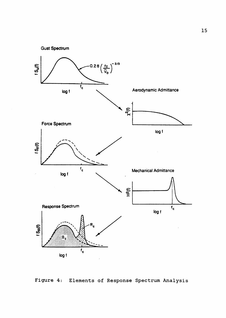
Several steps to obtain the mean scjuare value of
conductor response from the wind gust spectrum are shown in
Figure 4. The first step in the analysis involves the
transformation of the gust spectral density function, S (f),
into the force spectral density function, Sp(f), by
2 multiplying by the aerodynamic admittance function, x (f)-
The second step involves the determination of the response
spectral density function, S„(f), by multiplying the force
spectral density function by the mechanical admittance
2 function, H (f). The aerodynamic admittance function and
the mechanical admittance function are frecjuency response
functions. The third step is to calculate the mean square
value of the response, CT^, from the area under the response
spectrum. Once the RMS value of response, cjj, is obtained,
a peak value of the fluctuating response is determined by
Gust Spectrum
15
- 2 / 3
Force Spectrum
CO
Response Spectrum
Aerodynamic Admittance
logl
Mechanical Admittance
Figure 4: Elements of Response Spectrum Analysis
16
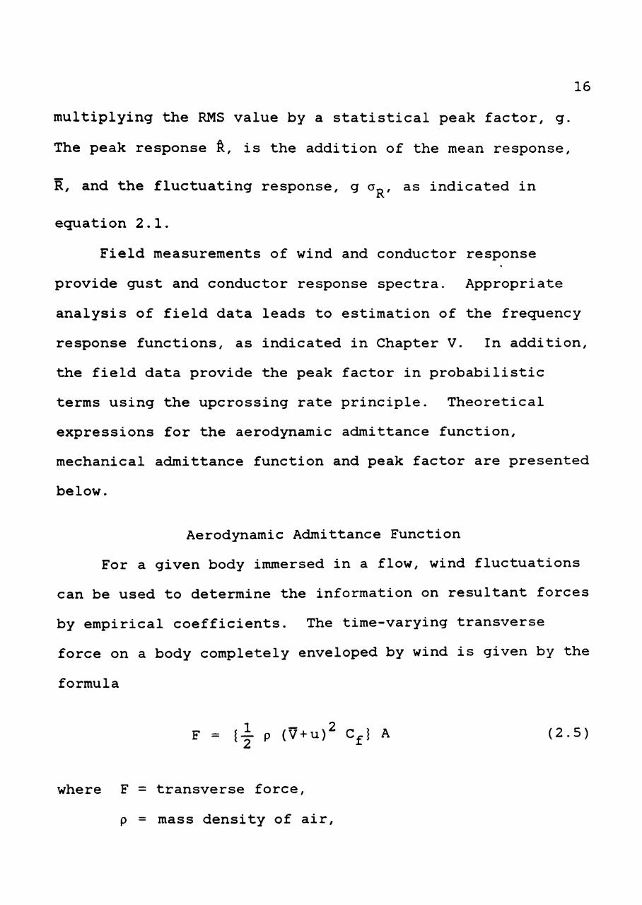
multiplying the RMS value by a statistical peak factor, g.
The peak response ft, is the addition of the mean response,
R, and the fluctuating response, <3 ^r^, as indicated in
ecjuation 2.1.
Field measurements of wind and conductor response
provide gust and conductor response spectra. Appropriate
analysis of field data leads to estimation of the frecjuency
response functions, as indicated in Chapter V. In addition,
tJie field data provide the peak factor in probabilistic
terms using the upcrossing rate principle. Theoretical
expressions for the aerodynamic admittance function,
mechanical admittance function and peak factor are presented
below.
Aerodynamic Admittance Function
For a given body immersed in a flow, wind fluctuations
can be used to determine the information on resultant forces
by empirical coefficients. The time-varying transverse
force on a body completely enveloped by wind is given by the
formula
F = [i. p (V + u)^ C^i A (2.5)
where F = transverse force,
p = mass density of air.
17
V = mean wind speed,
u = fluctuating component of wind speed,
C^ = force coefficient, and
A = area of exposure.
The time-varying fluctuating force is divided into two
components, mean force, F, and fluctuating force, F'. Then
ecjuation 2.5 can be expanded as
F -f F' = ^ p (V +2VU + U'') C^ A. (2.6)
2 If the term of the order u is neglected, the mean and
fluctuating forces can be separated as
1 -2 F = -i. p V C^ A (2.7)
and
F' = p V u C^ A. (2.8)
The power spectrum for fluctuating transverse force,
F', is then related to the gust spectrum as follows:
2 Sp(f) = (p V A C^) S^(f) (2.9)
or
_2
Sp(f) = ± ^ S^(f). (2.10)
V
18
Ecjuation 2.10, is valid over the range of frecjuencies
contained in the gust spectrum provided all effects remain
perfectly correlated. In practical conditions where gust
effects over the entire length of the conductor may not be
correlated, an adjustment factor or aerodynamic factor is
included in the ecjuation. This factor is called the
aerodynamic admittance function, x (f)/ and equation 2.10
becomes:
Sp(f) = ^ X^(f) S^(f)- (2.11)
The aerodynamic admittance function is a frecjuency
transfer function which transfers the gust spectral density
function to a force spectral density function. It accounts
for the correlation of gusts over the structure. The
distribution of gusts over the structure depends on the
relative size of the structure and the gusts. A large gust
totally enveloping the structure will be well correlated
over the structure, while small gusts acting over only a
portion of the structure are uncorrelated. In general,
low-frecjuency gusts are assumed to be correlated over the
2 structure; that is x (f) is assumed close to unity. The
2 value of X (f) fall below unity at frequencies in the range
19
of interest for the effects of winds on conductors. This
variation in aerodynamic admittance function as a function
of frecjuency is illustrated in Figure 4. The aerodynamic
admittance function for a structure is generally obtained
from wind tunnel tests (Blevins, 1977). In this study
coefficients of this function are obtained from the field
data (see Chapter V)-.
Mechanical Admittance Function
After the force spectral density function, Sp(f), is
obtained by means of ecjuation 2.11, the response spectral
density function, S„(f), is obtained by multiplying Sp(f) by
2 the mechanical admittance function, |H(f)| :
Sj (f) = |H(f)|2 Sp(f). (2.12)
2
The mechanical admittance function, |H(f)| , is
determined from an analysis using the stiffness, mass, and
damping characteristics of the structure. For a single
degree of freedom system, the mechanical admittance function
is the scjuare of the structural dynamic amplification
function; it is expressed as (Bendat, 1980):
H(f)|2 = J- ^ —^ (2.13)
k' f 2 2 f 2
o
20
where f = fundamental frecjuency,
C = damping ratio, and
k = spring constant.
The form of the mechanical admittance function is
illustrated in Figure 4. The resulting spectrum of the
response, shown in Figure 4, is peaked at the fundamental
frecjuency of the structure. This peak is the resonant
response of the structure at that frecjuency. One of the
major unknowns in the mechanical admittance function is the
dcunping ratio, C,. Damping can be due to structural and
material properties, and for wind response, aerodynamic
interaction. Structural damping can be assessed only from
experiments. A theoretical expression for aerodynamic
damping is presented in a subsecjuent section of this
chapter. In this study damping of conductors is determined
from field data; this is presented in Chapter V.
Peak Factor
Another important component in ecjuation 2.1 is the
statistical peak factor, g. Davenport (1977) has shown that
for a stationary random process, the statistics of the peak
response values may be represented by a Type I extreme-value
probability distribution. For this case the peak factor
21
corresponding to the peak response occurring in time period,
T, can be approximated as:
0.577 g = V2 In yT + ^•-^'' . (2.14)
V2 In yT
Where y is the cycling rate of the process; that is, the
number of times the mean response value is crossed per unit
time.
The peak factor has also been determined from the rate
of upcrossing. Melbourne (1975) used this principle of rate
of upcrossing as developed by Rice (1945) to analyze wind
tunnel aero-elastic model data.
Consider a continuous random process that can be
differentiated at least once. A sample function of the
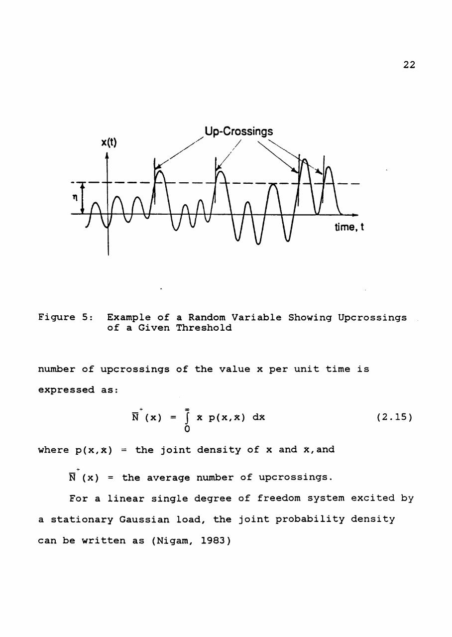
random process is shown in Figure 5. The crossings of the
level x(t)=Ti, with a positive slope (upcrossings) are shown
in the figure. The number of crossings of the level in the
time interval T is a random variable. For a long period of
time the expected or mean number of crossings will approach
some fixed value. Based on this average value, the average
crossing rate can be determined.
Rice (1945) showed that the average crossing rate can
be computed for any stationary random process x(t), if the
joint density distribution is known for x(t) and x(t) (the
sample functions of x(t) being dx(t)/dt). The average
22
Up-Crossings
time, t
Figure 5: Example of a Random Variable Showing Upcrossings of a Given Threshold
number of upcrossings of the value x per unit time is
expressed as:
N (x) = j X p(x,x) dx (2.15)
where p(x,x) = the joint density of x and x,and
N (x) = the average number of upcrossings.
For a linear single degree of freedom system excited by
a stationary Gaussian load, the joint probability density
can be written as (Nigam, 1983)
23
1 2 .2 P^""'^) = ?nn\ e x p [ - J L - - ^ l ( 2 . 1 6 )
X X
2 where a = mean scjuare of x, and
2 a = mean scjuare of x.
There is no covariance term a in the density equation
2.16 because x and x are assumed to be uncorrelated.
Substituting ecjuation 2.16 into ecjuation 2.15 and performing
the indicated integration yields
1 "x x^ N ( ) = ^ —^ e x p { - ^ l . (2.17)
2" ^x 2al
For a narrow band random process, the spectral energy
is centered close to the fundamental frecjuency, f , of the
structure. Thus ecjuation 2.17 can be written as (Reelect,
1969):
x^ N = f e x p l - ^ l - (2.18)
2^x
The cumulative probability distribution in terms of
upcrossings can be stated as
-* 2 P(>x) = EJ2LL = exp{--^l. (2.19)
^o 2ol
24
The upcrossing rate formulation is for a narrow band
vibration process. The upcrossing rate technicjue is applied
to the data of conductor response in Chapter V to obtain
probabilistic peak factor, assuming that the conductor
vibrates at its fundamental frecjuency (as indicated by data
in Chapter IV).
Wind Characteristics
Wind fluctuates randomly both in time and space. Wind
speed over a given time interval can be considered as
consisting of a mean wind speed and a fluctuating component.
Knowledge of both the mean wind speed and the fluctuating
component assists in evaluating wind loads on transmission
line conductors. The mean wind speed, wind profile,
turbulence intensity, and gust spectra are presented as part
of this chapter.
Mean Wind Speed
Mean wind speed is defined as an average wind speed for
a specified time interval. The numerical value of the mean
wind speed can have large variations depending on the
interval used for averaging the wind speed. A shorter
averaging time leads to a higher mean wind speed value,
while a longer averaging time leads to a smaller mean wind
speed value. This is primarily due to short gusts of high
wind speed that last for short periods of time.
25
The length of the record for which the mean value and
the RMS value of wind speed are determined is somewhat
arbitrary. The record should be long enough to reflect the
effects of low frecjuency components of mechanical turbulence
generated by the terrain roughness, but short enough so that
a reasonably stationary time history, free of significant
trends is obtained. Analysis of the power spectral
densities of wind speed provides the background for an
appropriate selection of the averaging time interval for
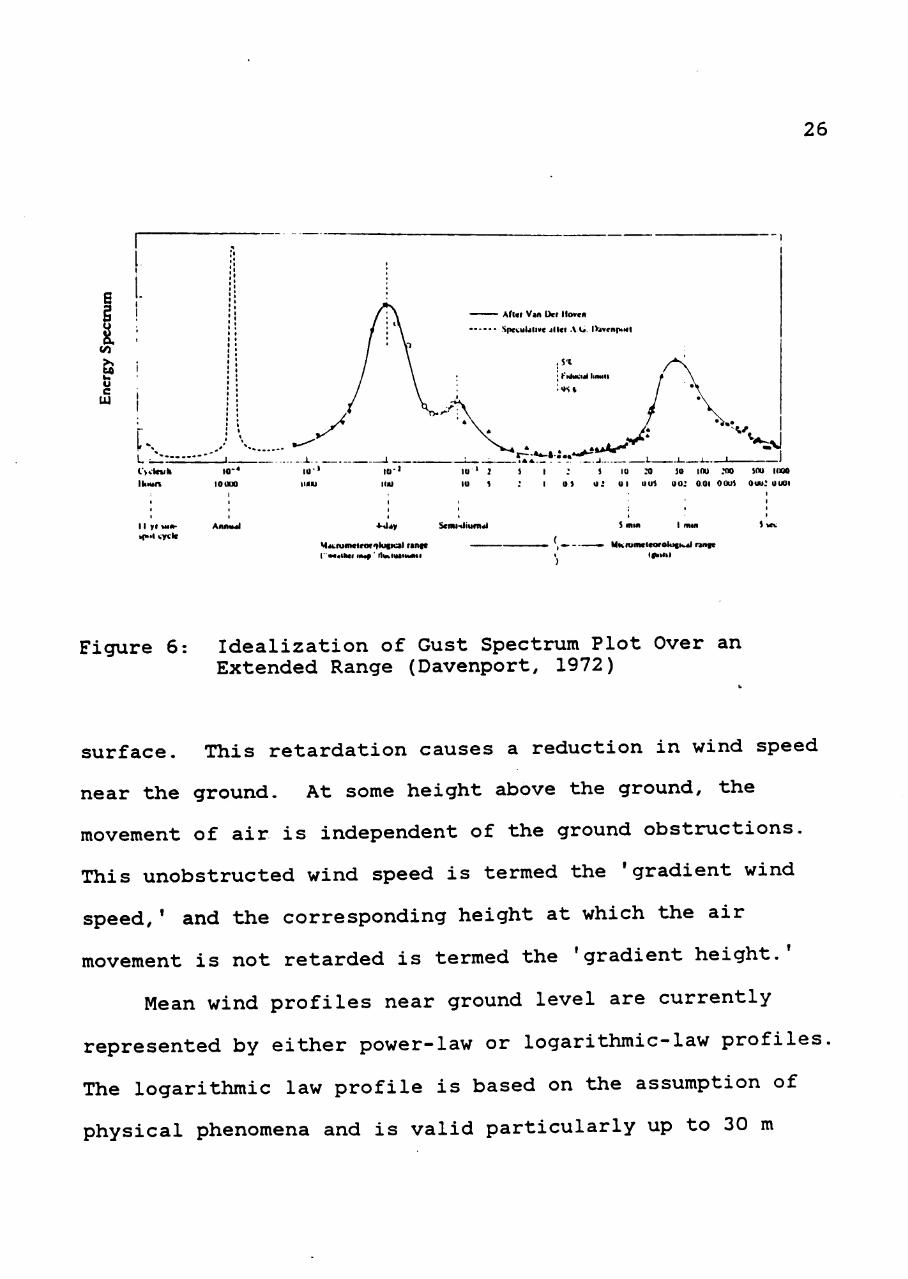
mean wind speed. The gust spectrum reveals that wind is
made up of two distinct types of air flow: (a)
macrometeorological or climate fluctuations, and (b)
micrometeorological fluctuations or gusts. These
fluctuations are separated by a stationary stable interval
(spectral gap) between 10 minutes and 1 hour, as indicated
in Figure 6. Based on this spectral gap, mean values
averaged over 10 minutes to 1 hour are optimum for stability
(Davenport, 1972). In this study, the wind speeds are
averaged over record length of 12 minutes.
Mean Wind Profile
An important characteristic of wind is the variation of
wind speed with height. The surface friction effects of the
ground retard the movement of air close to the ground
26 xt
rum
2S.
Ene
rgy
1 I 1
1. 1 t
i
1
1
u. Ivctevh
Ik iun
11 yt \u»-HK.I i;yck
I* ;!
•1 ii 1 t 1 * ( •
ii ! ;
n 1 1
to-«
lOUUO
1 t 1
ArniM.!
Afui V M Dcr llovcn
- - • Spck:uUli»« JIICI .\ ti. Oa«cnp<Ml
*-fi*r
M«;ruiii*irar<tlu|Hal ruifc r ' . . . t l l . ( m.^ ' llMlVtlMIHI
Scnutliufn.!
MkiunwicafolofivJ ruifc IfKMtl
Figure 6: Idealization of Gust Spectrum Plot Over an Extended Range (Davenport, 1972)
surface. This retardation causes a reduction in wind speed
near the ground. At some height above the ground, the
movement of air is independent of the ground obstructions.
This unobstructed wind speed is termed the 'gradient wind
speed,' and the corresponding height at which the air
movement is not retarded is termed the 'gradient height.'
Mean wind profiles near ground level are currently
represented by either power-law or logarithmic-law profiles
The logarithmic law profile is based on the assumption of
physical phenomena and is valid particularly up to 30 m
27
above ground (Simiu, 1984). The power-law profile is
empirical and is assumed to be valid up to gradient height
(approximately 500 m). The power-law profile is primarily
used in structural analysis and design, because of its
simplicity. It is essential to determine the wind profile
at a particular site, so that the mean wind speed at
effective height of structure can be determined. Power-law
is used in this study, and is briefly described below.
The power-law profile was developed by Davenport
(1960). He modifiecj the exponential profile developed by
Brunt (1952) to obtain a mean wind speed profile. In
horizontally homogeneous terrain, it is assumed that the
power-law is valid with a constant exponent (a) up to the
gradient height, Z . Both gradient height and power-law y
exponent are functions of the terrain roughness. The mean
wind profile is expressed as
Ii£l = (-?-)" (2.20)
where V(z) = mean wind speed at height, z,
V = mean wind speed at gradient height, Z , and
a = power-law exponent.
The power-law is used in both the American National
Standard ANSI A 58.1 (1982) and in the National Building
28
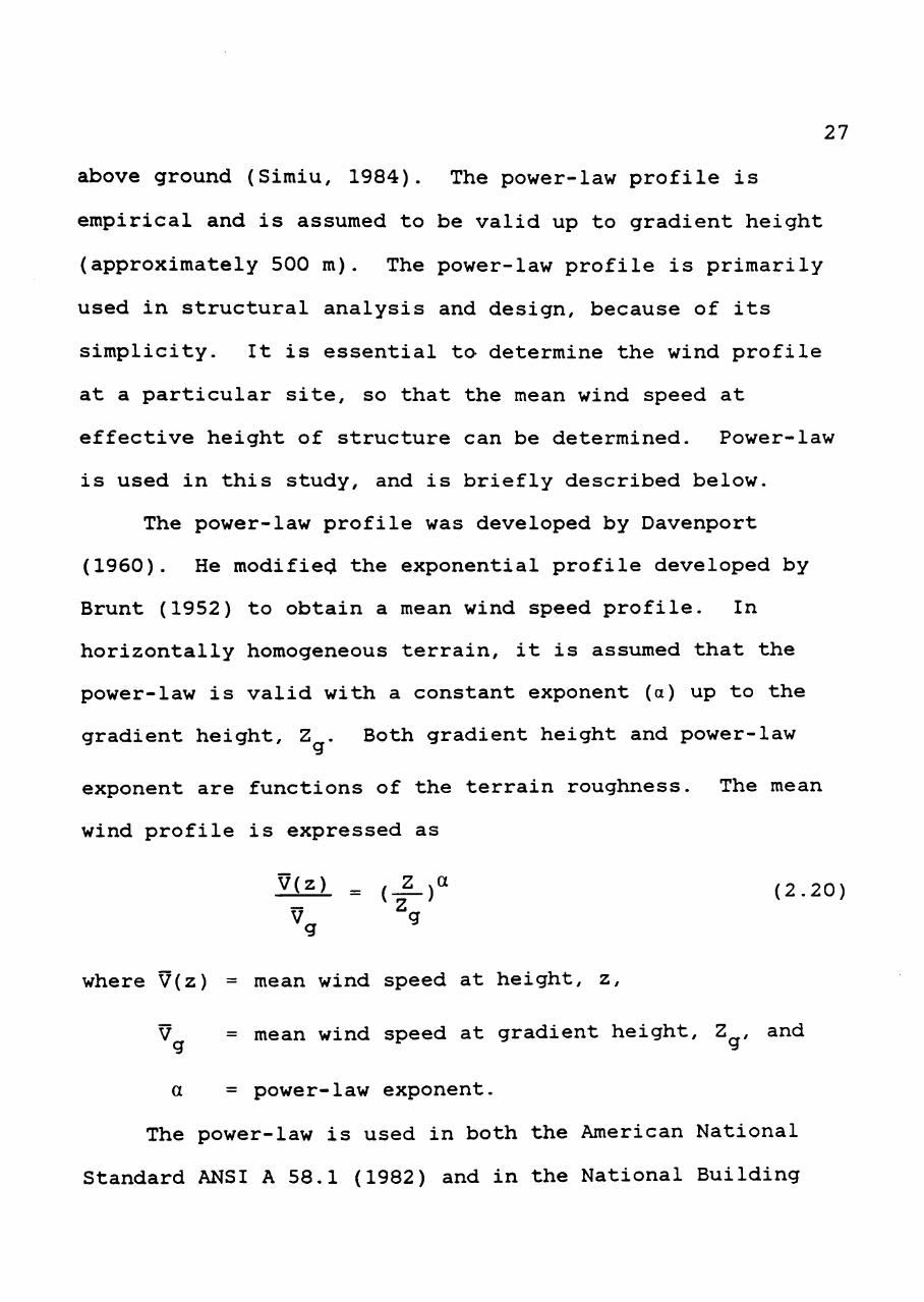
Code of Canada (NRCC, 1980). Typical values of the gradient
height, Z , and the power-law exponent, a, for different
terrains, as specified by ANSI (1982), are summarized in
Table 1.
TABLE 1
Typical Values for Gradient Height and Power-Law Exponent (ANSI, 1982)
Terrain Category
Coastal Areas
Open Farmland
Forest/Suburban
City Centers
Gradient He ight(ft)
Z g 700
900
1200
1500
Power Law Exponent
a
0.10
0.14
0.22
0.33
Turbulence Characteristics
The fluctuating part of wind is termed as the
turbulence. The turbulence present in the wind flow is due
to the ground roughness characteristics of the terrain over
which it is passing or due to thermally-induced convection
or both. The turbulence due to ground roughness is known as
mechanical turbulence and that due to heat convection is
29
known as convective turbulence. Depending on the relative
importance of convective to mechanical turbulence, the
stability conditions of the atmosphere are classified as
stable, neutral, and unstable (Simiu, 1985). The extreme
winds in which structural engineers are interested are
categorized as neutral stability conditions. In a neutrally
stable condition, the temperature related buoyancy forces
and resulting vertical air motions are minimum. For
engineering purposes, it is generally assumed that neutral
atmospheric stability conditions can be assumed for wind
speeds higher than 20 mph. Details of atmospheric neutral
conditions are discussed in detail by Kancharla (1987).
Analysis of turbulence includes determination of the
turbulence intensity and the gust spectrum. Of these two,
the turbulence intensity expression is simpler. It
indicates relative amplitudes of the fluctuations compared
to the mean wind speed. A complete representation of
fluctuating components of wind is the gust spectrum, which
gives the distribution of the mean scjuare over the frecjuency
domain. The gust spectrum is useful in assessing dynamic
response of structures. Both representations of turbulence
characteristics are discussed below.
30
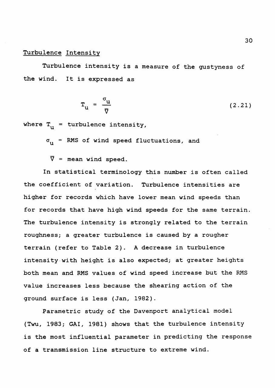
Turbulence Intensity
Turbulence intensity is a measure of the gustyness of
the wind. It is expressed as
T^ = -^ (2.21) V
where T = turbulence intensity,
a^ = RMS of wind speed fluctuations, and
V = mean wind speed.
In statistical terminology this number is often called
the coefficient of variation. Turbulence intensities are
higher for records which have lower mean wind speeds than
for records that have high wind speeds for the same terrain.
The turbulence intensity is strongly related to the terrain
roughness; a greater turbulence is caused by a rougher
terrain (refer to Table 2). A decrease in turbulence
intensity with height is also expected; at greater heights
both mean and RMS values of wind speed increase but the RMS
value increases less because the shearing action of the
ground surface is less (Jan, 1982).
Parametric study of the Davenport analytical model
(Twu, 1983; GAI, 1981) shows that the turbulence intensity
is the most influential parameter in predicting the response
of a transmission line structure to extreme wind.
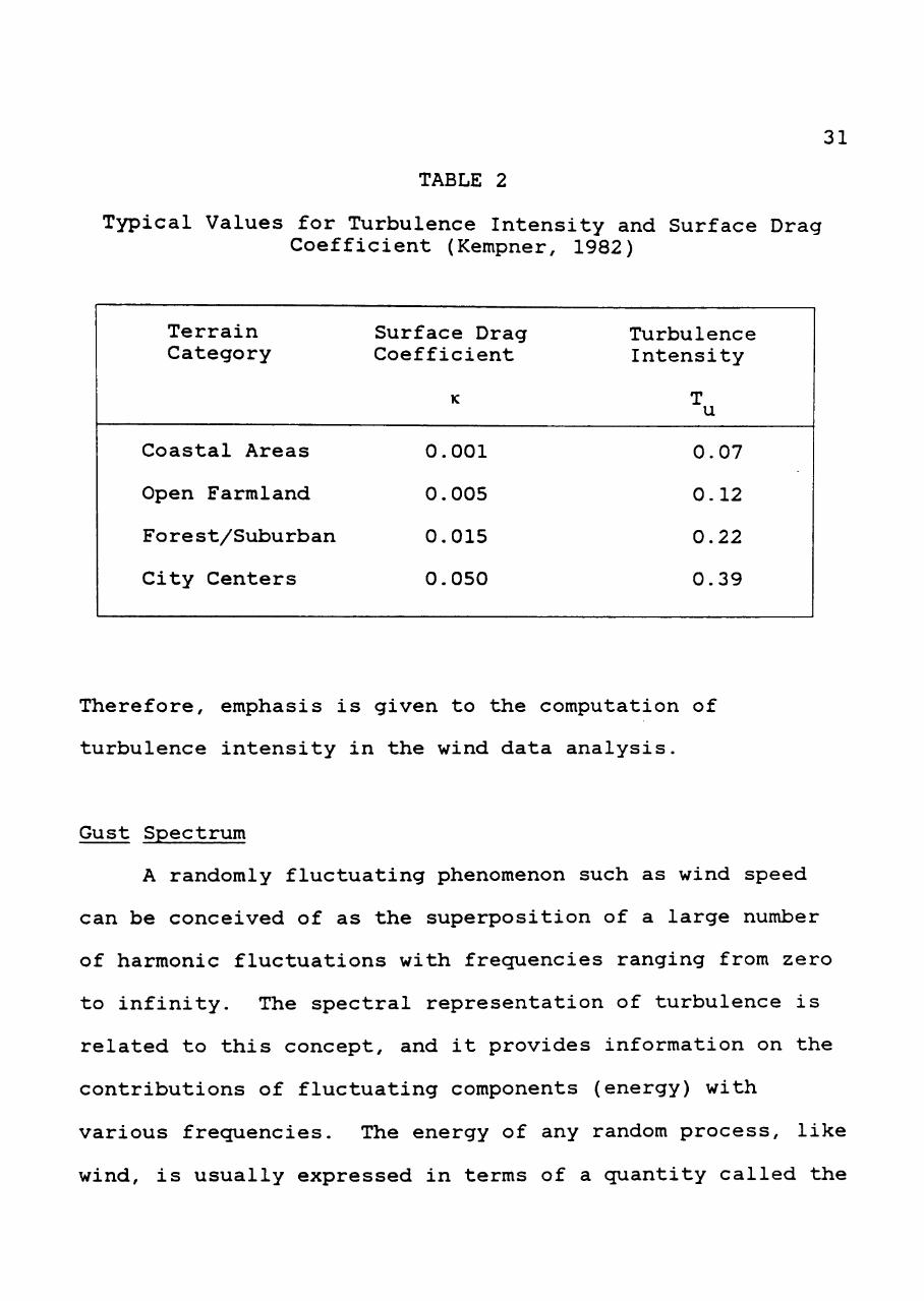
31
TABLE 2
Typical Values for Turbulence Intensity and Surface Drag Coefficient (Kempner, 1982)
Terrain Category
Coastal Areas
Open Farmland
Forest/Suburban
City Centers
Surface Drag Coefficient
0.
0.
0.
0.
K
001
005
015
050
Turbulence Intensity
T u
0.
0.
0.
0.
L
07
12
22
39
Therefore, emphasis is given to the computation of
turbulence intensity in the wind data analysis.
Gust Spectrum
A randomly fluctuating phenomenon such as wind speed
can be conceived of as the superposition of a large number
of harmonic fluctuations with frecjuencies ranging from zero
to infinity. The spectral representation of turbulence is
related to this concept, and it provides information on the
contributions of fluctuating components (energy) with
various frecjuencies. The energy of any random process, like
wind, is usually expressed in terms of a cjuantity called the
32
'Power Spectral Density (PSD).' The PSD at any particular
frecjuency, f, may be considered as the average fluctuating
wind power passing a fixed point when the wind as a random
process is filtered by a narrow band filter centered at f.
In the dynamic analysis of structures subjected to gust
loading, significant dynamic amplification of the response
may occur at a resonant frequency, i.e., when the natural
frecjuencies of vibration of the structure and of the wind
match (Simiu, 1985). Flexible structures like conductors
can have dynamic amplification of the response because the
fluctuating component of wind has a fair amount of power at
frecjuencies of structural vibration. On the other hand, if
the natural frecjuencies of vibration of the tower structures
are higher than 1 Hz, the dynamic amplification of the
response of the tower will be small because power in the
gust spectrum at those frecjuencies (see Figure 13, page 72)
is very small.
There are more than a dozen specific wind speed
spectrum ecjuations developed for meteorological and
engineering purposes. Some of these spectral ecjuations are
discussed by Kim (1977). For neutral atmospheric
conditions, wind turbulence is generated by the surface
shear stress. It follows that the magnitude of the PSD
should be proportional to the scjuare of the frictional
33
velocity. The analytical model for the gust spectrum used
in this study was developed by Kaimal (1978).
In general, the spectral energy of gusts is a function
of the wave-length, —, of the wind fluctuations and the
height, h, above the ground. The analytical form suggested
by Kaimal for the horizontal gust spectrum for height to
•f v> wave length ratios greater than one-half ( >0.5) is given
V
as:
f S„(f) ^ = A ^ *
f h
V '^ (2.22)
where S (f) = spectral density of gusts at frecjuency f.
u^= friction velocity, (^KV^Q)
K = surface drag coefficient,
(typical values are shown in Table 2)
V..Q= mean wind speed at 10 m height,
V = mean wind speed at height h,
h = height above ground, and
A, n = constants.
Constants A and n represent the amplitude and exponent
values of Kaimal's gust spectrum. For neutral atmospheric
34
conditions, A=0.3 and n=2/3 are suggested by Kaimal.
Ecjuation 2.22 is useful for describing the gust
spectrum in the high frecjuency range (low wave lengths) and
for heights limited to the first few tens of meters. Kaimal
also presents other forms of the gust spectrum which are
valid for lower frecjuencies and for unstable atmospheric
conditions.
Davenport Analytical Model
On the basis of Davenport's analytical model (1980),
the peak response, ft, of a conductor due to fluctuating
winds is represented by ecjuation 2.1. Davenport's model
provides an analytical expression for the RMS, cjp, and
suggests a peak factor value, g, in the range 3.5-4.0.
Validation and refinement of the expression for the RMS are
part of this study.
The mean scjuare fluctuating response of a conductor is
the area under the response spectrum. The area under the
response spectrum can be considered as the summation of the
background response, B , and the resonant response, R . The
c c
background response is caused by gust with various
durations, whereas resonant response is caused by gust
frecjuencies at the natural frecjuencies of the conductor.
The total mean scjuare fluctuating response of the conductor
is given as:
^R = ^c ^ ^c
35
(2.23)
where B = the mean scjuare background response, and
R = the mean scjuare resonant response.
The expressions for background and resonant responses
consider wind properties such as mean wind speed, turbulence
intensity and gust spectrum and structural properties such
as frecjuency of vibration and damping. Ecjuations for
background and resonant responses of the conductor response
have been developed by Davenport (1980) and are given below.
The ecjuations are:
B_ = e P E^ c 1 + 0.81(-ii-l
^s
(2.24)
2 — 2 R = 6 P E^ c c 0.323A h. 1 , o ^,-(n-H) (2.25)
1 f7 = mean wind pressure; —pV C^ where P
e = the influence coefficient which translates
E =
the force to response; for conductor transverse
response is the product of L and d,
exposure factor at the effective height of
36
the conductor; which is twice the turbulence
intensity,
Lg = transverse scale of turbulence,
C^ = conductor force coefficient,
p = mass density of air,
C = conductor aerodynamic damping as a ratio
to the critical damping,
V = mean wind speed at the effective height
of the conductor,
f^ = fundamental frequency of the conductor
(horizontal sway),
A, n = Kaimal's gust spectrum constants,
c = narrow band correlation coefficient of
turbulence, with a typical value of 8,
L = effective conductor span,
d = conductor diameter, and
h = effective conductor height.
The background and resonant terms for conductor
response are calculated using ecjuations 2.24 and 2.25. The
mean scjuare value of fluctuating response is obtained using
ecjuation 2.23. Some of the assumptions made by Davenport in
deriving the simplified expressions for conductor response
are discussed by Mehta (Criswell, 1987).
37
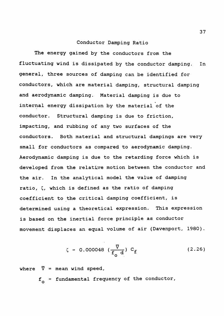
Conductor Damping Ratio
The energy gained by the conductors from the
fluctuating wind is dissipated by the conductor damping. In
general, three sources of damping can be identified for
conductors, which are material damping, structural damping
and aerodynamic damping. Material damping is due to
internal energy dissipation by the material of the
conductor. Structural damping is due to friction,
impacting, and rubbing of any two surfaces of the
conductors. Both material and structural dampings are very
small for conductors as compared to aerodynamic damping.
Aerodynamic damping is due to the retarding force which is
developed from the relative motion between the conductor and
the air. In the analytical model the value of damping
ratio, C/ which is defined as the ratio of damping
coefficient to the critical damping coefficient, is
determined using a theoretical expression. This expression
is based on the inertial force principle as conductor
movement displaces an ecjual volume of air (Davenport, 1980).
C = 0.000048 (^ ) C^ (2.26) o
where V = mean wind speed,
f = fundamental frequency of the conductor.
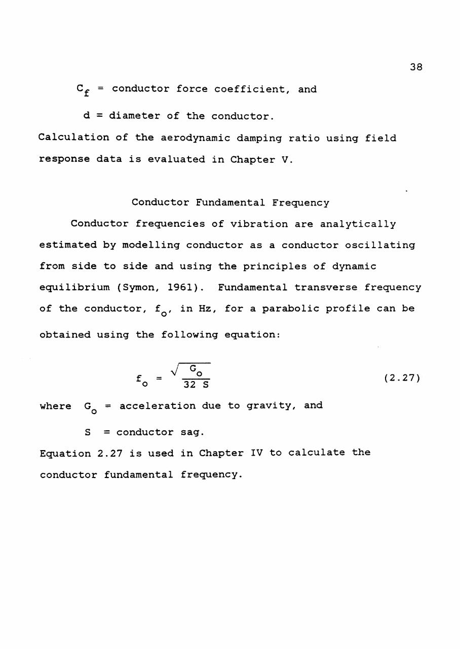
38
C^ = conductor force coefficient, and
d = diameter of the conductor.
Calculation of the aerodynamic damping ratio using field
response data is evaluated in Chapter V.
Conductor Fundamental Frecjuency
Conductor frecjuencies of vibration are analytically
estimated by modelling conductor as a conductor oscillating
from side to side and using the principles of dynamic
ecjuilibrium (Symon, 1961). Fundamental transverse frequency
of the conductor, f , in Hz, for a parabolic profile can be
obtained using the following ecjuation:
JG f = ^ (2.27) o 32 S ^ '
where G = acceleration due to gravity, and
S = conductor sag.
Ecjuation 2.27 is used in Chapter IV to calculate the
conductor fundamental frecjuency.
CHAPTER III
FIELD DATA
Full-scale data used in this study were collected by
the Bonneville Power Administration (BPA). Since 1976, BPA
has conducted several projects to study wind load response
of transmission line systems by collecting and analyzing
wind and response related data on test lines in the field.
Transmission tower and conductor wind response data were
collected on an energized 500 kV single circuit transmission
line. An instrumentation system was used to measure wind
speed, wind direction, insulator swing, insulator load, and
tower member stresses.
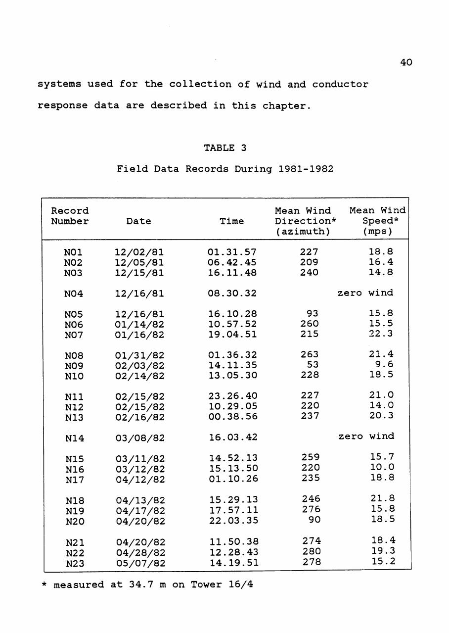
During the period of December 1981 through May 1982,
BPA collected twenty-three separate recordings of wind and
the transmission line response with twelve-minute duration.
Dates, times, and mean wind speeds and direction of these
twenty-three records are shown in Table 3. These recordings
are used in the study presented here. Each record is
numbered by Nxx, where xx is the secjuence number of
occurrence of high winds. Data utilized in this study are
limited to wind and conductor response data. The site
characteristics, the instruments and the data accjuisition
39
40
systems used for the collection of wind and conductor
response data are described in this chapter.
TABLE 3
Field Data Records During 1981-1982
Record Number
NOl N02 N03
N04
N05 N06 N07
N08 N09 NIC
Nil N12 N13
N14
N15 N16 N17
N18 N19 N20
N21 N22 N23
Date
12/02/81 12/05/81 12/15/81
12/16/81
12/16/81 01/14/82 01/16/82
01/31/82 02/03/82 02/14/82
02/15/82 02/15/82 02/16/82
03/08/82
03/11/82 03/12/82 04/12/82
04/13/82 04/17/82 04/20/82
04/20/82 04/28/82 05/07/82
Time
01.31.57 06.42.45 16.11.48
08.30.32
16.10.28 10.57.52 19.04.51
01.36.32 14.11.35 13.05.30
23.26.40 10.29.05 00.38.56
16.03.42
14.52.13 15.13.50 01.10.26
15.29.13 17.57.11 22.03.35
11.50.38 12.28.43 14.19.51
Mean Wind Direction* (azimuth)
227 209 240
93 260 215
263 53
228
227 220 237
259 220 235
246 276 90
274 280 278
Mean Wind Speed* (mps)
18.8 16.4 14.8
zero wind
15.8 15.5 22.3
21.4 9.6 18.5
21.0 14.0 20.3
zero wind
15.7 10.0 18.8
21.8 15.8 18.5
18.4 19.3 15.2
* measured at 34.7 m on Tower 16/4
41
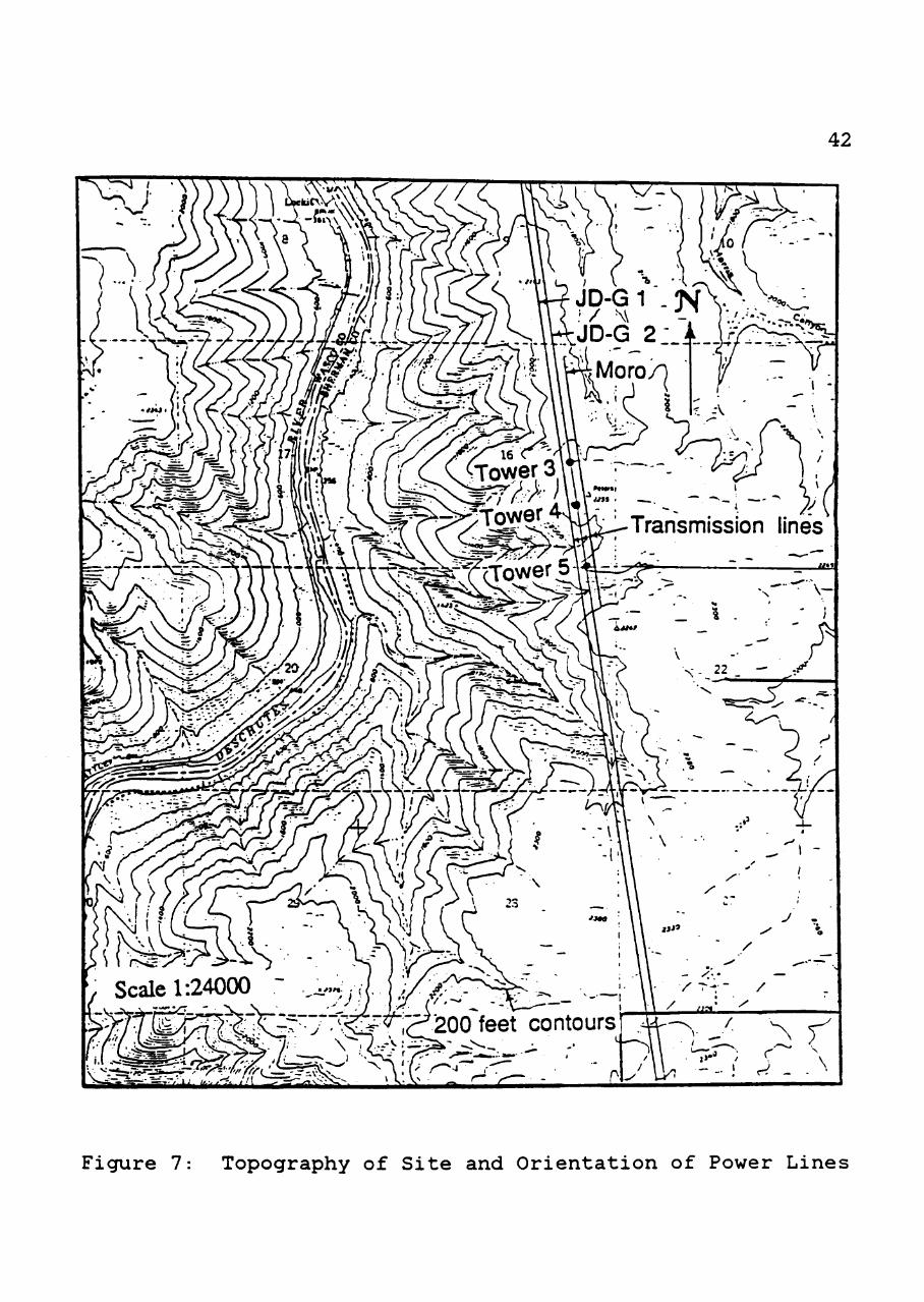
Description of Test Site
The test site is located at Moro, Oregon, 56 kilometers
southeast of Dalles, Oregon (east of the Cascade Mountains).
The general topography in the vicinity of the test lines is
shown in Figure 7. As observed from the contours in the
figure, the deep Deschutes river canyon is just west of the
site. The test line is essentially located on the rim of
the canyon. To the east of the test lines is a flat terrain
which is uncultivated land containing grass with some
shrubs. The test lines are approximately 1500 m to the east
and 500 m above the elevation of the Deschutes river.
As indicated in Figure 7, the test site includes three
lines running almost north-south and approximately 8 degrees
west of true north (Kempner, 1981). The first 2 lines east
of the Deschutes river are 500 kV energized lines, called
John-Day Grizzly (JD-G) 1 and 2. A non-energized mechanical
test line (also referred to as the Moro test line) parallels
the other lines. JD-G lines 1 and 2 are 45.7 m apart,
whereas the distance between JD-G line 2 and the mechanical
test line is 38.1 m. Towers at the site (on JD-G line 2)
are numbered from 1 to 5, Tower 1 being the tower at the
northern end of the site. The instrumented tower is Tower
4, part of the John Day-Grizzly (line 2) system. It is
referred to as Tower JD-G 16/4 or simply Tower 16/4 because
it is located on mile 16 of JD-G line 2.
42
Figure 7: Topography of Site and Orientation of Power Lines
43
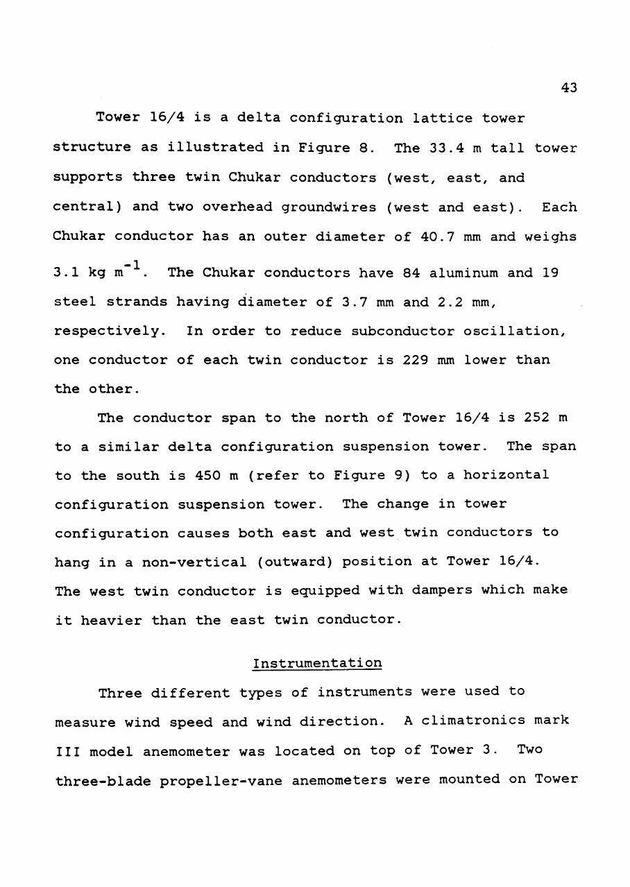
Tower 16/4 is a delta configuration lattice tower
structure as illustrated in Figure 8. The 33.4 m tall tower
supports three twin Chukar conductors (west, east, and
central) and two overhead groundwires (west and east). Each
Chukar conductor has an outer diameter of 40.7 mm and weighs
3.1 kg m~ . The Chukar conductors have 84 aluminum and 19
steel strands having ciiameter of 3.7 mm and 2.2 mm,
respectively. In order to reduce subconductor oscillation,
one conductor of each twin conductor is 229 mm lower than
the other.
The conductor span to the north of Tower 16/4 is 252 m
to a similar delta configuration suspension tower. The span
to the south is 450 m (refer to Figure 9) to a horizontal
configuration suspension tower. The change in tower
configuration causes both east and west twin conductors to
hang in a non-vertical (outward) position at Tower 16/4.
The west twin conductor is ecjuipped with dampers which make
it heavier than the east twin conductor.
Instrumentation
Three different types of instruments were used to
measure wind speed and wind direction. A climatronics mark
III model anemometer was located on top of Tower 3. Two
three-blade propeller-vane anemometers were mounted on Tower
44
West conductor
Anemomeler (34.7 m)
Load cell and Swing angle indicators
41 mm diameter
Figure 8: Schematic of Tower 16/4
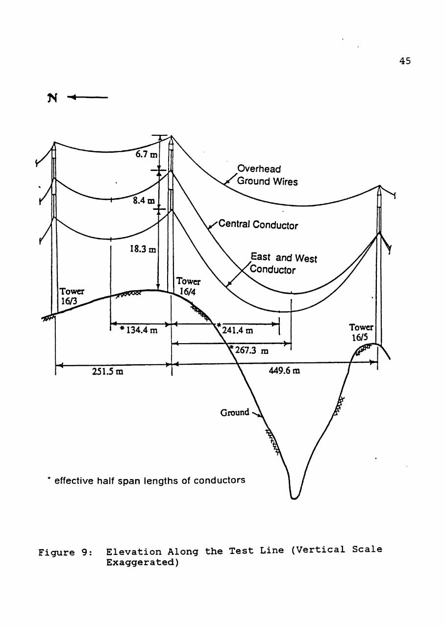
N -^
45
effective half span lengths of conductors
Figure 9: Elevation Along the Test Line (Vertical Scale Exaggerated)
46
16/4, as shown in Figure 8. One was located on top of the
tower at a height of 34.7 m. The second unit was located on
the northwest tower leg at a height of 10 m and it projected
out 2.3 m north of the tower. Two four-blade propeller-vane
anemometers were installed on top of Towers 4 and 5. The
three-blade propeller-vane anemometer has a threshold speed
of 1.7 mps and a distance constant of approximately 4.6 m.
The threshold value is the stall speed of the unit. The
distance constant is the wind passage recjuired for 63%
recovery from a step change in wind speed. The wind
instruments ecjuipped with internal heaters to allow for
winter operation. Wind direction is indicated by azimuth
readings in degrees referenced to true north. The wind
direction is such that a zero degree reading corresponds to
true north and a clockwise rotation represents an increase
in the wind direction reading.
The load cells and swing angle indicators measured the
magnitude and direction of the conductor and overhead ground
wire loads that transfer to the tower structure. The
instruments were installed in the linkage between the
insulator string and the tower. All conductors and ground
wires were instrumented with one axial load cell and two
swing angle indicators. The swing angle indicators measured
longitudinal and transverse swings of the insulators.
47
Baldwin-Lima-Hamilton (BLH) strain gage load cells were
used to measure axial loads. BLH Type T3P1 load cells,
rated at 5000 pounds, were used for the overhead ground
wires and BLH Type T2P1 load cells, rated at 20,000 pounds,
were used for the conductors. Humphrey pendulum swing angle
indicators, model CP17-0601-1, were used to measure the
longitudinal (along the line) and transverse (perpendicular
to tihe line) swings of the insulator string. These units
measure up to ±45 degrees of swing from the zero (vertical)
position with a resolution of 0.2 degrees (Kempner, 1977).
Valid data from these units are restricted to 2 Hz or less
because of the unit natural frecjuency of 3.2 Hz, as
suggested by Kempner (1980). The load cells and swing angle
indicators were calibrated in the laboratory and checked in
the field after installation.
Data Acquisition
Data was collected by the Moro UHV mechanical test
program data accjuisition system (Kempner, 1979). The data
accjuisition system consisted of a PDP-11/10 mini-computer
with 12 K memory, an ADAC Model 600-11 Data Accjuisition
System, a Digi Data Controller/Formater, a 7-track magnetic
tape unit, and a teletype. The data accjuisition system was
housed in an instrument trailer located 30 m southwest of
48
the Tower 16/4. The system was set up to record from 256
channels of instrumentation.
RecordincT Procedure
Several selected channels constituted a recording mode,
which were selected to capture a static or dynamic
phenomenon of interest. The data used in the present study
were recorded in Mode 22. Mode 22 was designed for
recording wind and the response of Tower 16/4. It consisted
of 38 channels of instrumentation. The instrumentation on
Tower 16/4 included 12 strain gages, 5 load cells, 10 swing
angle indicators, and 2 wind instruments. The remaining
channels provide readings from the anemometers mounted on or
adjacent to Towers 2, 3, 4, and 5 on the Moro mechanical
test line. A complete list of the channels with a
description of each is given in Table 4 (Norville, 1985).
The PDP-11/10 computer was used to monitor wind
conditions and to initiate recordings when prescribed
conditions were met. Prescribed information was entered
into and stored in the computer prior to placing the data
accjuisition system on-line. This information included
channel identification, date and time of recording, number
of samples, mode number, calibration and offset factors for
each channel (Kempner, 1979). This information was written
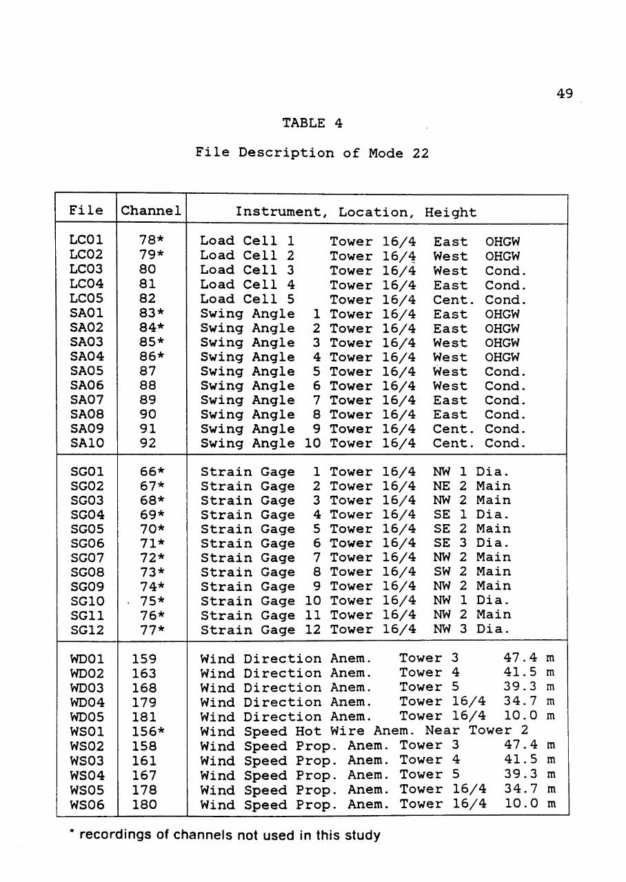
TABLE 4
File Description of Mode 22
49
File
LCOl LC02 LC03 LC04 LC05 SAOl SA02 SA03 SA04 SA05 SAO 6 SA07 SA08 SA09 SAIO
SGOl SG02 SG03 SG04 SG05 SG06 SG07 SG08 SG09 SGIO SGll SG12
WDOl WD02 WD03 WD04 WD05 WSOl WS02 WS03 WS04 WS05 WS06
Channel
78* 79* 80 81 82 83* 84* 85* 86* 87 88 89 90 91 92
66* 67* 68* 69* 70* 71* 72* 73* 74*
. 75* 76* 77*
159 163 168 179 181 156* 158 161 167 178 180
Instrument,
Load Cell 1 Load Cell 2 Load Cell 3 Load Cell 4 Load Cell 5 Swing Angle Swing Angle Swing Angle Swing Angle Swing Angle Swing Angle Swing Angle Swing Angle Swing Angle Swing Angle
Strain Gage Strain Gage Strain Gage Strain Gage Strain Gage Strain Gage Strain Gage Strain Gage Strain Gage Strain Gage Strain Gage Strain Gage
1 2 3 4 5 6 7 8 9 10
1 2 3 4 5 6 7 8 9 10 11 12
Wind Direction Wind Direction Wind Directi on Wind Direction Wind Direction Wind Speed Hot Wind Speed E Wind Speed E Wind Speed E
Location,
Tower Tower Tower Tower Tower Tower Tower Tower Tower Tower Tower Tower Tower Tower Tower
Tower Tower Tower Tower Tower Tower Tower Tower Tower Tower Tower Tower
Anem. Anem. Anem. Anem. Anem.
16/4 16/4 16/4 16/4 16/4 16/4 16/4 16/4 16/4 16/4 16/4 16/4 16/4 16/4 16/4
16/4 16/4 16/4 16/4 16/4 16/4 16/4 16/4 16/4 16/4 16/4 16/4
Height
East West West East Cent. East East West West West West East East Cent. Cent.
NW 1 NE 2 NW 2 SE 1 SE 2 SE 3 NW 2 SW 2 NW 2 NW 1 NW 2 NW 3
Tower 3 Tower 4 Tower 5
OHGW OHGW Cond. Cond. Cond. OHGW OHGW OHGW OHGW Cond. Cond. Cond. Cond. Cond. Cond.
Dia. Main Main Dia. Main Dia. Main Main Main Dia. Main Dia.
47.4 m 41.5 m 39.3 m
Tower 16/4 34.7 m Tower 16/4 10.0 m
Wire Anem. Near Tower 2 'rop. Anem. Tower 3 »rop. Anem. Tower 4 »rop. Anem. Tower 5
47.4 m 41.5 m 39.3 m
Wind Speed Prop. Anem. Tower 16/4 34.7 m Wind Speed E »rop. Anem. Tower 16/4 10.0 m
recordings of channels not used in this study
50
as a heading on the magnetic tape preceding a strong wind
recording.
Triggering of this recording mode was automatic when
the wind speed was equal to or greater than 18 mps for one
minute and the temperature was ecjual to or greater than 4
degrees Celsius. Once triggered, the recording mode sampled
the data for 10 or 12 continuous minutes, depending upon the
sampling rate. After a recording period, the mode had one
hour waiting period before another trigger was allowed.
Two data sampling rates were used in recording the data
for mode 22. The sampling and recording rates were limited
by the size of the computer memory and the speed of the
magnetic tape unit. Sampling rates of 10 samples per second
(sps) and 20 sps were used in collecting data. Channels 66
through 79 (LCOl, LC02 and SG01-SG12) were monitored at 20
sps; all other channels were sampled at 10 sps. All the
data utilized in the study presented here had sampling rates
of 10 sps and were collected for 12-minute durations.
Description of Recordings
The recordings that were collected in the field are
summarized in Table 3. The winds at the test site during
the period of data collection were predominantly from the
west, with only three records of east winds. Two zero wind
51
records were collected for initializing conductor and tower
response data. Mean wind speed values ranged from 9.6 to
22.3 mps. Mean wind directions varied from almost normal
(transverse) to transmission line to 55 degrees from the
normal. The terrain over which the wind traversed in each
recording segment depended on the wind direction. These
variations in wind speed, wind direction and terrain caused
inherent variability in the collected data. Field
experiments depend on the vagaries of nature; they cannot be
duplicated or repeated. The inherent variability in field
data and the inability to repeat the experiment suggest that
results from the analysis should be based on an ensemble of
data and that some scattering of results is to be expected.
CHAPTER IV
FIELD DATA ANALYSIS
Analysis of field data recjuires that the validity and
accuracy of the wind and conductor response data be checked.
It is expected that results of field data will have a
certain amount of scattering. This scattering can be due to
an inherent variation in field data as well as a variation
in the data measuring system. To the extent possible, wind
data and conductor response data are checked for consistency
and accuracy.
The analytical procedure to predict the response of
conductors recjuires knowledge of wind characteristics such
as the mean wind speed, power-law exponent of wind profile,
turbulence intensity, and Kaimal's gust spectrum constants.
These characteristics are determined from the field data and
are subsecjuently used in the analytical procedure.
Field recorded conductor response can be compared with
predicted values in terms of mean response and fluctuating
response. Effective force coefficients that relate to mean
response are determined for each record of the field data.
Fluctuating response, as indicated in Chapter II, is a
combination of background response and resonant response.
52
53
These responses can be assessed from response spectra of the
field measured values. The conductor response spectrum of
transverse loads recorded by load cells is discussed in this
chapter. The discussion relates to background response and
resonant response. Comparisons of recorded fluctuating
responses with predicted values from the analytical
procedure are presented in the next chapter. In addition,
an assessments of the peak factor, admittance function and
damping from the recorded data are presented in next
chapter.
Validity of Wind Data
Wind speeds and directions were recorded at five
locations, namely on top of Towers 3, 4, 5, and 16/4, and at
10.0 m on Tower 16/4. Tower 4 is within 38 m of Tower 16/4,
while Towers 3 and 5 are several hundred meters from the
other two towers (see Figure 9).
The mean azimuth and root mean scjuare (RMS) of wind
direction for each record for these five locations are shown
in Table 5. Data were recorded at 10 sps for 12 minutes in
each record. One observation in Table 5 is the consistency
in mean azimuth value for the three instruments located at
the tops of Towers 4, 5, and 16/4. The differences in mean
values for these three instruments are less than 12 degrees.
54
and in most cases less than 6 degrees. The two instruments,
one at 34.7 m height on Tower 16/4 and one at 41.5 m on top
of Tower 4, give mean wind directions within 4 degrees for
winds from several different azimuths. This consistency in
mean azimuth values provides credibility to the wind
direction instruments and the data accjuisition system.
The mean azimuth values for the instrument at 10.0 m
height on Tower 16/4 are erratic when compared with the
values from the other instruments for records NOl through
N13 (see Table 5). The difference in mean azimuth value is
as high as 44 degrees. Such a large difference in wind
direction between records for instruments on the same tower
located at 10.0 m and at 34.7 m cannot be explained from
physical phenomena. Ekman's spiral suggests that a
deviation in wind direction occurs close to ground, but the
deviation in a 25 m difference in height should be less than
6 degrees (Simiu, 1985). This large difference in wind
direction for the instrument at 10.0 m on Tower 16/4 casts
doubt in its wind data for records NOl through N13; these
records are not used in further analysis. The remaining
records (N15 through N23) for this instrument appear to give
reasonable results. The wind instrument on top of Tower 3
also gives mean azimuth values higher by 10 to 20 degrees
than the other instruments on a consistent basis. Wind data
from Tower 3 are not needed in the analysis.
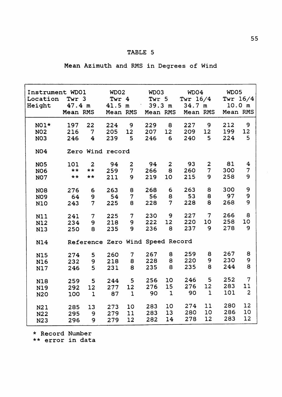
TABLE 5
Mean Azimuth and RMS in Degrees of Wind
55
Instrument WDOl Location Height
NOl* N02 N03
N04
N05 N06 N07
NOB N09 NIC
Nil N12 N13
N14
N15 N16 N17
Twr 3 47.4 m
Mean RMS
197 216 246
Zero
101 * *
•k-k
276 64
243
241 234 250
Refe
274 232 246
22 7 4
Wind
2 * *
*-k
6 9 7
7 9 8
rence
5 9 5
WD02 Twr 41.5 Mean
224 205 239
4 m RMS
9 12 5
record
94 259 211
263 54
225
225 218 235
Zero
260 218 231
2 7 9
8 7 8
7 9 9
Wind
7 8 8
WD03 Twr 39.3
Mean
229 207 246
94 266 219
268 56
228
230 222 236
5 m RMS
8 12 6
2 8 10
6 8 7
9 12 8
WD04 Twr 16/4 34.7 Mean
227 209 240
93 260 215
263 53
228
227 220 237
Speed Record
267 228 235
8 8 8
259 220 235
m RMS
9 12 5
2 7 9
8 8 8
7 10 9
8 9 8
WD05 Twr 10.
Mear
212 199 224
81 300 258
300 97
268
266 258 278
267 230 244
16/4 0 m L RMS
9 12 5
4 7 9
9 9 9
8 10 9
8 9 8
N18 N19 N20
N21 N22 N23
259 292 100
285 295 296
5 12 1
13 9 9
244 277 87
273 279 279
5 12 1
10 11 12
256 276 90
283 283 282
10 15 1
10 13 14
246 276 90
274 280 278
5 12 1
11 10 12
252 283 101
280 286 283
7 11 2
12 10 12
* Record Number ** error in data
56
The mean wind speed value for each record for the five
wind speed instruments is tabulated in Table 6. One
observation in Table 6 is the consistency in mean wind speed
value for the four instruments located on the tops of Towers
3, 4, 5, and 16/4. The values among these instruments are
within 15%. The variation in mean speed values may be due
to a combination of two reasons. First, the instruments are
at slightly different heights above the ground; wind speed
is expected to be higher as height increases. The second
reason may be that the distances between the towers are
several hundred meters; so the terrain over which the wind
travels can be different. This combination of variation in
terrain and height of instrument can account for variations
in mean wind speed values. The instrument at 41.5 m height
on Tower 4 recorded 4% higher mean wind speed than that at
34.7 m height on Tower 16/4 on an average (see Table 6).
Since Towers 4 and 16/4 are only 38 m apart with no terrain
modulations, it is reasonable to assume that a height
difference accounts for the small difference in mean wind
speed values. This consistency in mean speed values
provides credibility to the wind speed instruments and the
measurements.
The difference between the mean wind speeds at 10.0 m
and at 34.7 m on Tower 16/4 is very small for records NOl
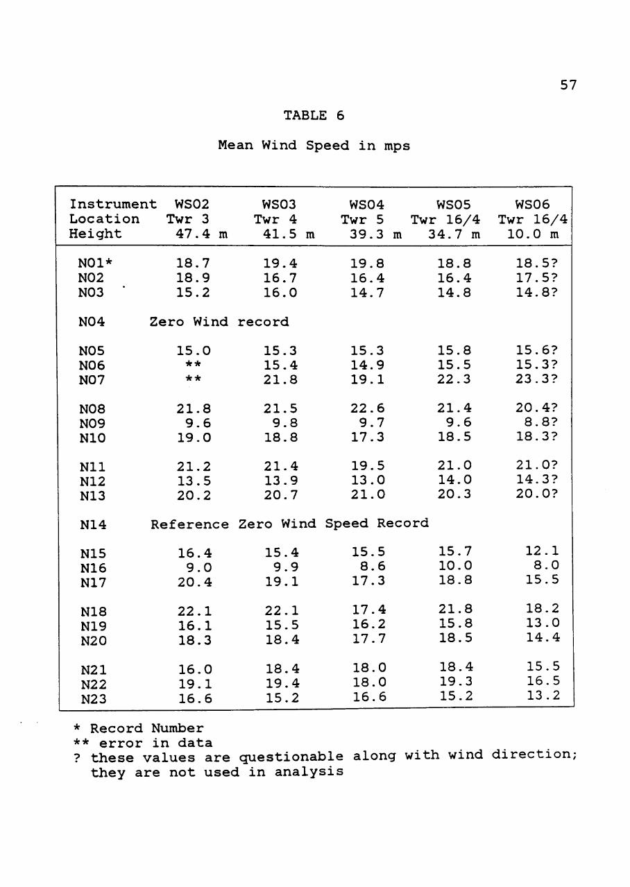
TABLE 6
Mean Wind Speed in mps
57
Instrument WS02 Location Twr 3 Height 47.4 m
WS03 Twr 4 41.5 m
WS04 WS05 Twr 5 Twr 16/4 39.3 m 34.7 m
WS06 Twr 16/4 10.0 m
NOl* N02 N03
N04
N05 NO 6 N07
NOB N09 NIC
Nil N12 N13
N14
N15 N16 N17
N18 N19 N20
18.7 18.9 15.2
19.4 16.7 16.0
19.8 16.4 14.7
18.8 16.4 14.8
Zero Wind record
15.0 * *
* *
21.8 9.6 19.0
21.2 13.5 20.2
15.3 15.4 21.8
21.5 9.8 18.8
21.4 13.9 20.7
15.3 14.9 19.1
22.6 9.7 17.3
19.5 13.0 21.0
Reference Zero Wind Speed Record
16.4 9.0
20.4
22.1 16.1 18.3
15.4 9.9 19.1
22 15 18
1 5 4
15.5 8.6 17.3
17.4 16.2 17.7
15.7 10.0 18.8
N21 N22 N23
16, 19, 16.
0 1 6
18.4 19.4 15.2
18 18 16
0 0 6
18.5? 17.5? 14.8?
15.8 15.5 22.3
21.4 9.6 18.5
21.0 14.0 20.3
15.6? 15.3? 23.3?
20.4? 8.8? 18.3?
21.0? 14.3? 20.0?
12.1 8.0 15.5
21.8 15.8 18.5
18.4 19.3 15.2
18.2 13.0 14.4
15.5 16.5 13.2
* Record Number ** error in data ? these values are cjuestionable along with wind direction; they are not used in analysis
58
through N13. In a few records, the instrument at 10.0 m
height shows higher mean wind speed values than that at 34.7
m height. Wind speed at 34.7 m on Tower 16/4 is more
consistent with the other instruments on top of Towers 3, 4,
and 5. This casts some doubt on the wind speeds of records
NOl through N13 measured at 10.0 m height on Tower 16/4;
these records are not used for further analysis.
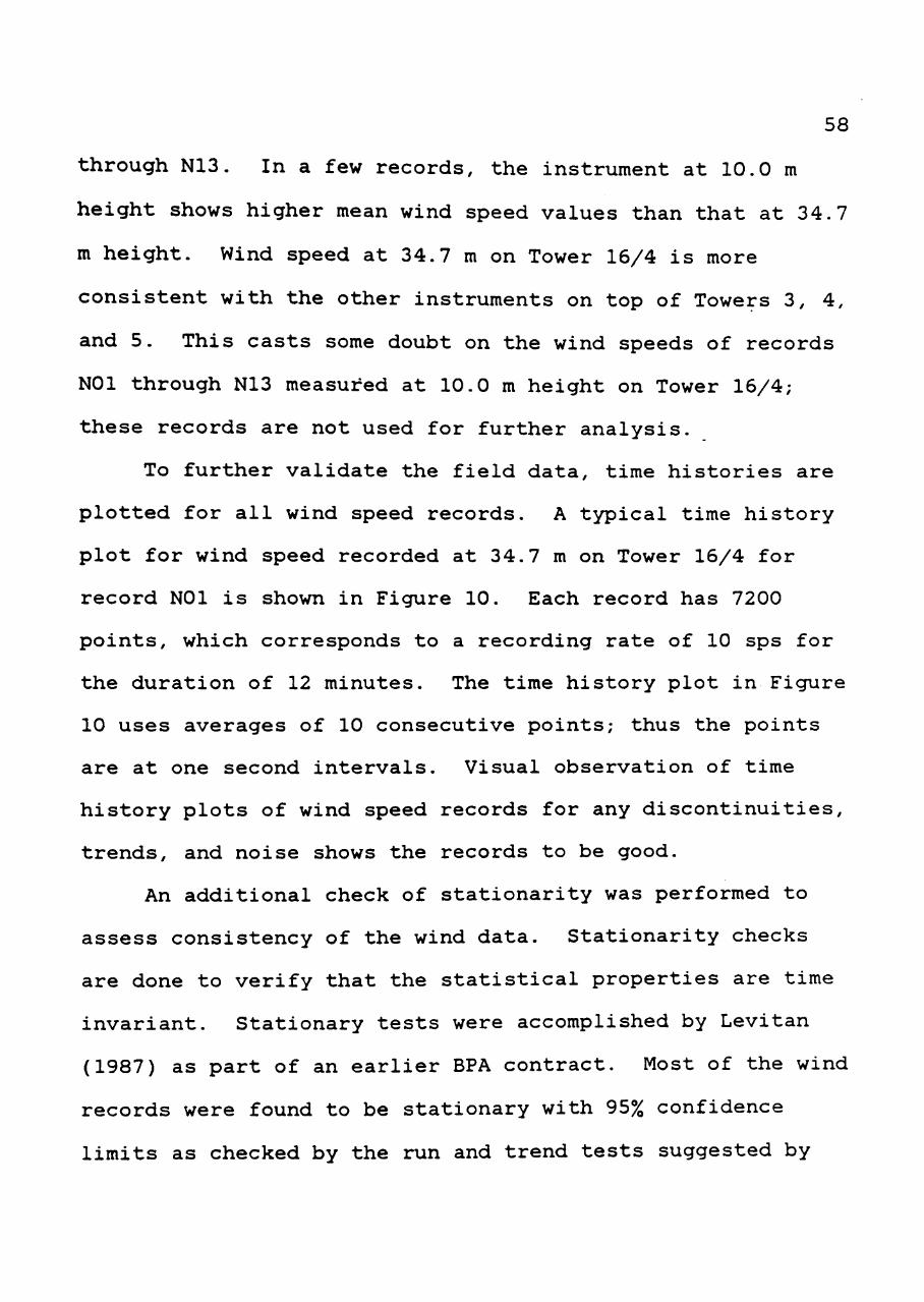
To further validate the field data, time histories are
plotted for all wind speed records. A typical time history
plot for wind speed recorded at 34.7 m on Tower 16/4 for
record NOl is shown in Figure 10. Each record has 7200
points, which corresponds to a recording rate of 10 sps for
the duration of 12 minutes. The time history plot in Figure
10 uses averages of 10 consecutive points; thus the points
are at one second intervals. Visual observation of time
history plots of wind speed records for any discontinuities,
trends, and noise shows the records to be good.
An additional check of stationarity was performed to
assess consistency of the wind data. Stationarity checks
are done to verify that the statistical properties are time
invariant. Stationary tests were accomplished by Levitan
(1987) as part of an earlier BPA contract. Most of the wind
records were found to be stationary with 95% confidence
limits as checked by the run and trend tests suggested by
59
Time (minutes)
Figure 10: Time History Plot of Wind Speed for Record NOl at 34.7 m on Tower 16/4
Bendat and Piersol (1966). These stationary test are not
discussed in this study. Finally, as a part of the
validation of the data, a power spectrum plot for each
record was generated. These plots would reveal, in the
frecjuency domain, any electrical or other sources of noise
in the data. Details of these power spectrum plots are
discussed in subsecjuent sections. In general, most of the
wind speed and wind direction records appear to be valid.
60
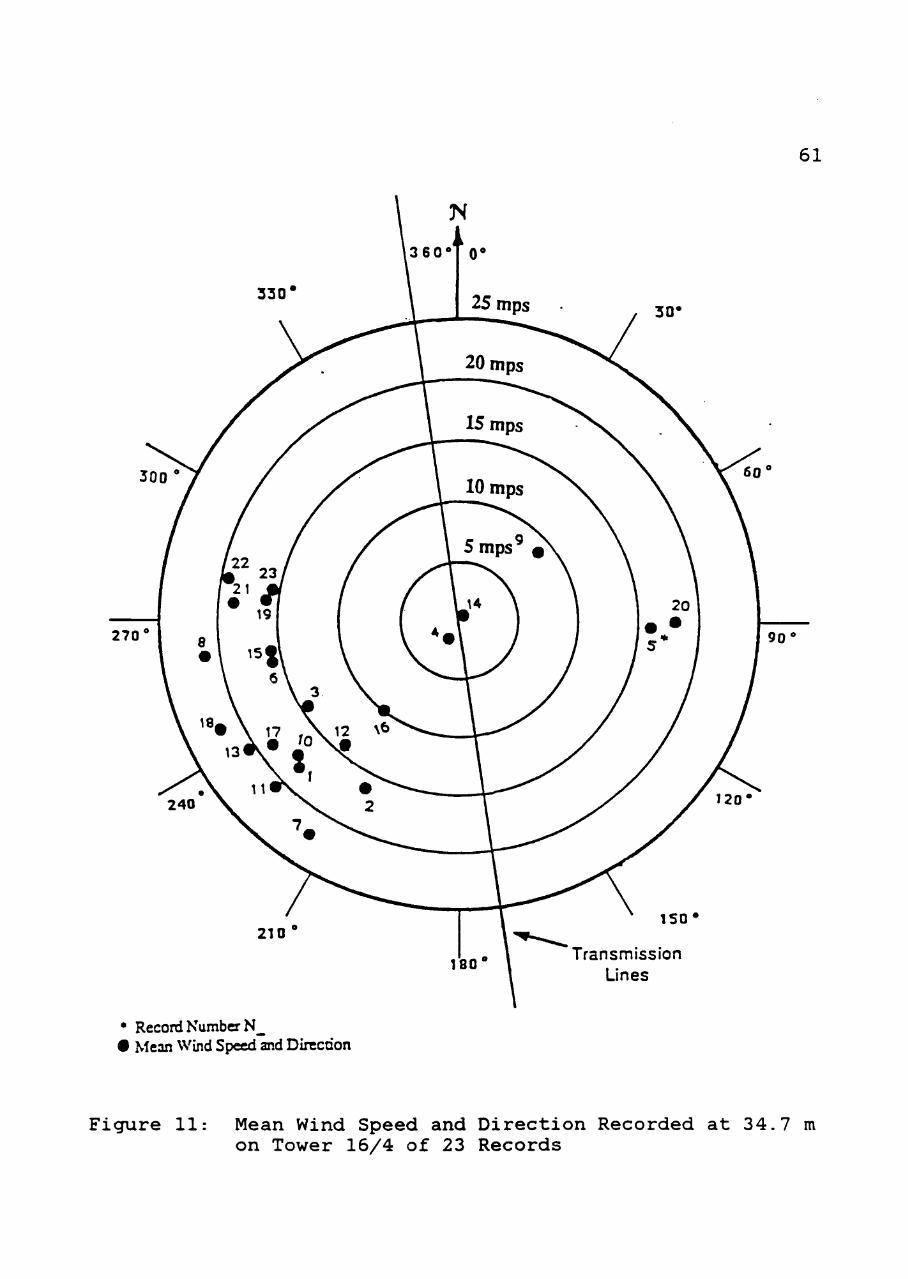
The mean wind speed and mean wind direction for each
record at 34.7 m height on Tower 16/4 are shown in Figure
11. There are eighteen west wind records, three east wind
records and two zero wind records. Wind directions vary
from almost normal to the transmission line to as high as 55
degrees of yaw angle (see Figure 11). The mean wind speed
values are 10 mps or higher for all records, except for the
zero wind records.
Two zero wind records (N04 and N14) were collected in
near calm or zero wind conditions. Based on a review of the
data of these two records, N14 is selected as a reference
record to assess conductor response.
Wind speed on top of Tower 16/4 (at 34.7 m height) is
used as the reference wind speed record. The reference wind
speed record is important to determine the wind speed at the
effective height of the conductor. The wind speeds at the
effective heights are determined using the reference wind
speed and vertical wind profile.
Power-Law Exponent for Wind Profile
The wind speed profile is assessed using mean wind
speed records of instruments located at 10.0 m and 34.7 m
heights on Tower 16/4 and at 41.5 m height on Tower 4.
Since Towers 16/4 and 4 are only 38 m apart with no terrain
6 1
• Record Number N_ • Mean Wind Speed and Direction
Figure 11: Mean Wind Speed and Direction Recorded at 34.7 m on Tower 16/4 of 23 Records
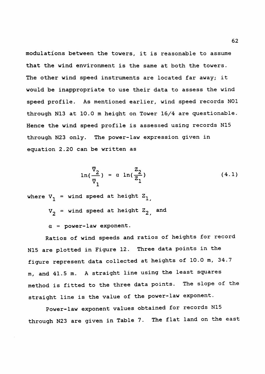
62
modulations between the towers, it is reasonable to assume
that the wind environment is the same at both the towers.
The other wind speed instruments are located far away; it
would be inappropriate to use their data to assess the wind
speed profile. As mentioned earlier, wind speed records NOl
through N13 at 10.0 m height on Tower 16/4 are cjuestionable.
Hence the wind speed profile is assessed using records N15
through N23 only. The power-law expression given in
ecjuation 2.20 can be written as
V^ Z, ln(-f.) = a ln(-^) (4.1)
Vl
where V, = wind speed at height Z^
V2 = wind speed at height Z2 and
a = power-law exponent.
Ratios of wind speeds and ratios of heights for record
N15 are plotted in Figure 12. Three data points in the
figure represent data collected at heights of 10.0 m, 34.7
m, and 41.5 m. A straight line using the least squares
method is fitted to the three data points. The slope of the
straight line is the value of the power-law exponent.
Power-law exponent values obtained for records N15
through N23 are given in Table 7. The flat land on the east
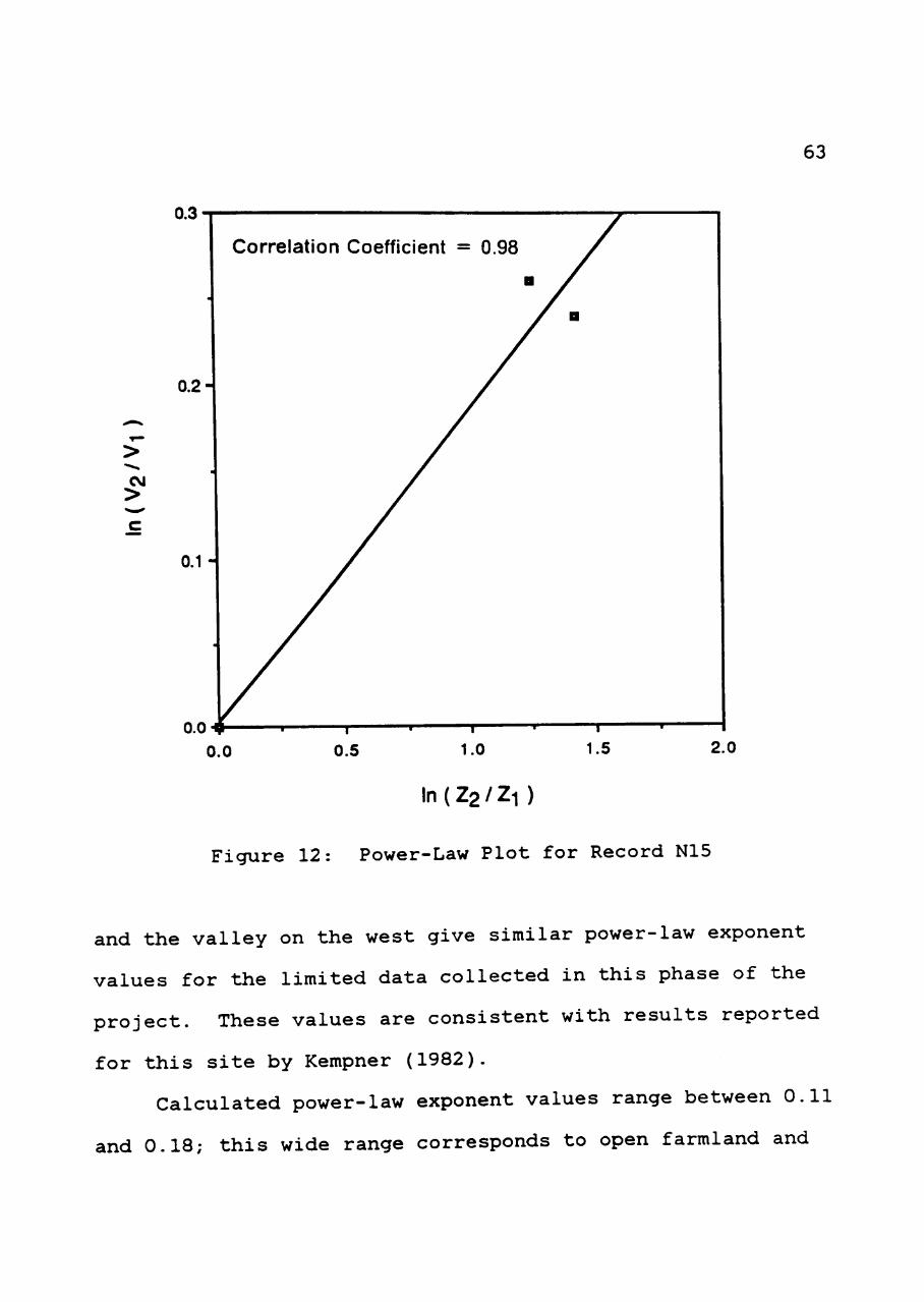
63
CVi >
ln(Z2/Zi)
Figure 12: Power-Law Plot for Record N15
and the valley on the west give similar power-law exponent
values for the limited data collected in this phase of the
project. These values are consistent with results reported
for this site by Kempner (1982).
Calculated power-law exponent values range between 0.11
and 0.18; this wide range corresponds to open farmland and
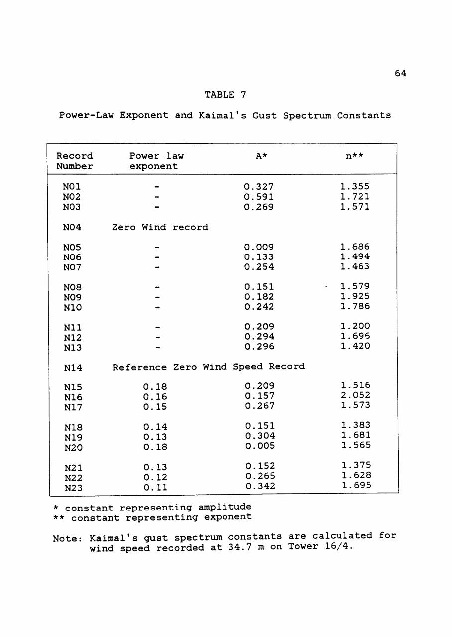
64
TABLE 7
Power-Law Exponent and Kaimal's Gust Spectrum Constants
Record Number
NOl N02 N03
N04
N05 NO 6 NO 7
N08 N09 NIO
Nil N12 N13
N14
N15 N16 N17
N18 N19 N20
N21 N22 N23
Power 1 aw exponent
_
-
-
Zero Wind
_
-
-
.
-.
-
^
-
-
Reference
0.18 0.16 0.15
0.14 0.13 0.18
0.13 0.12 0.11
record
Zero Wind
A*
0.327 0.591 0.269
0.009 0.133 0.254
0.151 0.182 0.242
0.209 0.294 0.296
Speed Record
0.209 0.157 0.267
0.151 0.304 0.005
0.152 0.265 0.342
n**
1.355 1.721 1.571
1.686 1.494 1.463
• 1.579 1.925 1.786
1.200 1.696 1.420
1.516 2.052 1.573
1.383 1.681 1.565
1.375 1.628 1.695
* constant representing amplitude ** constant representing exponent
Note: Kaimal's gust spectrum constants are calculated for wind speed recorded at 34.7 m on Tower 16/4.
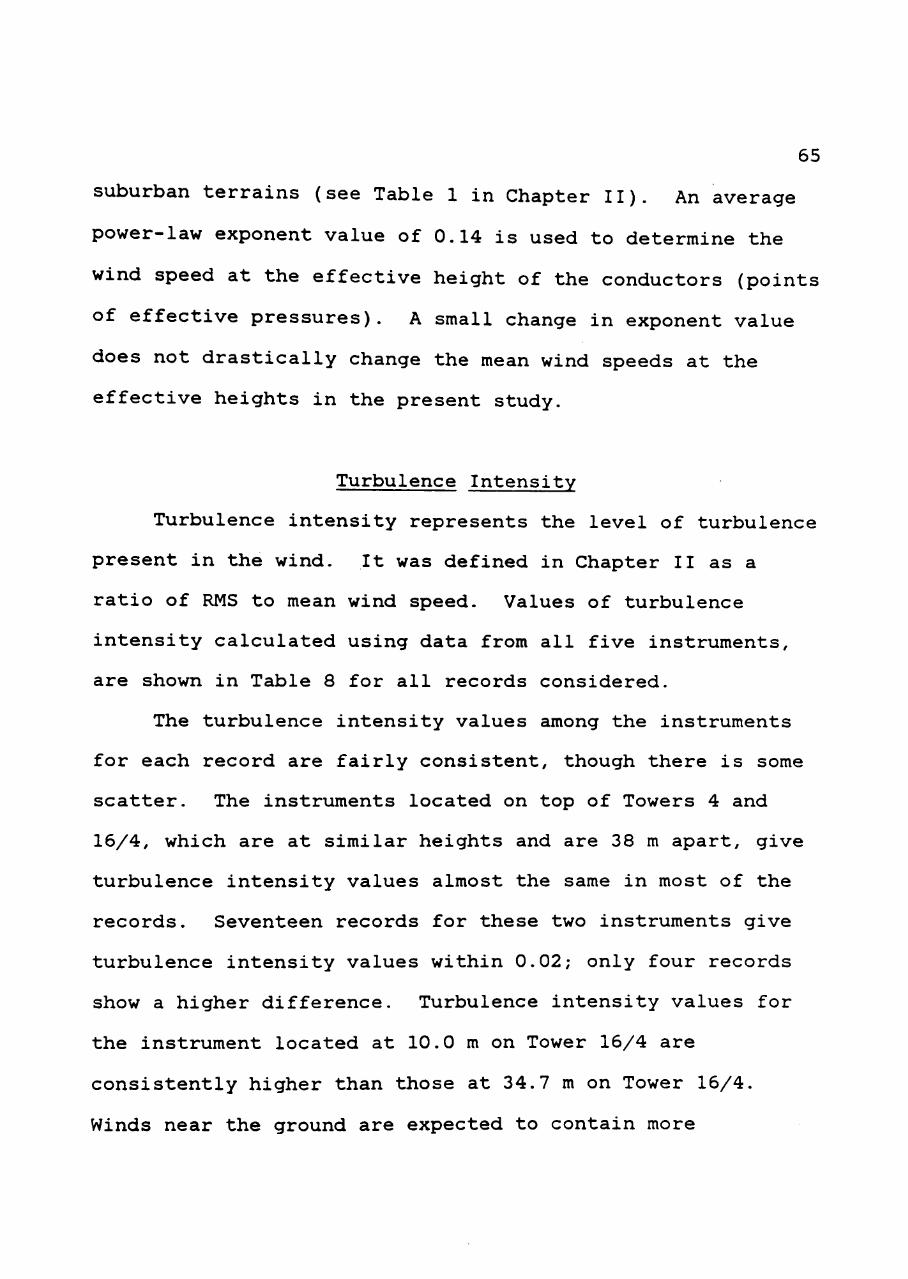
65
suburban terrains (see Table 1 in Chapter II). An average
power-law exponent value of 0.14 is used to determine the
wind speed at the effective height of the conductors (points
of effective pressures). A small change in exponent value
does not drastically change the mean wind speeds at the
effective heights in the present study.
Turbulence Intensity
Turbulence intensity represents the level of turbulence
present in the wind. It was defined in Chapter II as a
ratio of RMS to mean wind speed. Values of turbulence
intensity calculated using data from all five instruments,
are shown in Table 8 for all records considered.
The turbulence intensity values among the instruments
for each record are fairly consistent, though there is some
scatter. The instruments located on top of Towers 4 and
16/4, which are at similar heights and are 38 m apart, give
turbulence intensity values almost the same in most of the
records. Seventeen records for these two instruments give
turbulence intensity values within 0.02; only four records
show a higher difference. Turbulence intensity values for
the instrument located at 10.0 m on Tower 16/4 are
consistently higher than those at 34.7 m on Tower 16/4.
Winds near the ground are expected to contain more
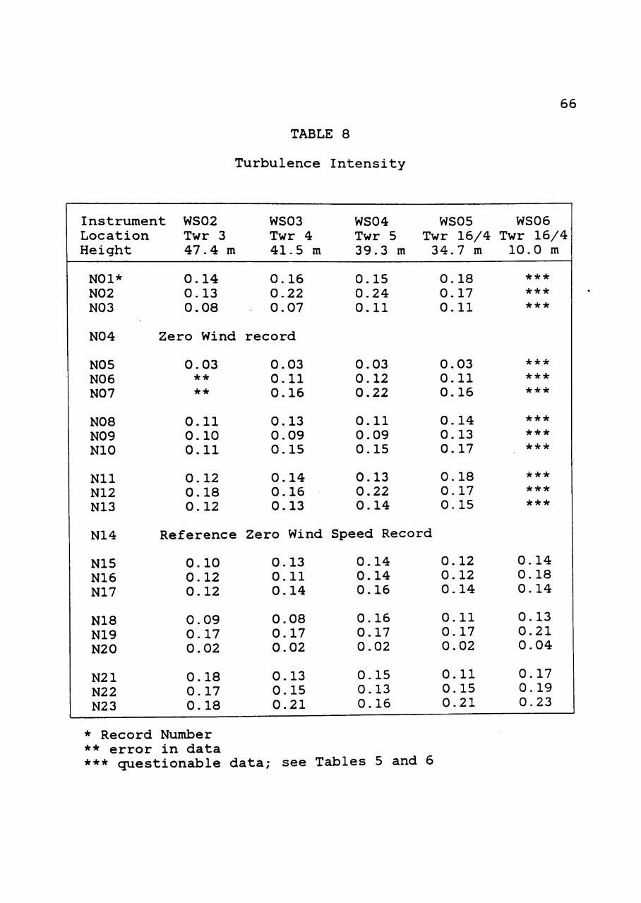
TABLE 8
Turbulence Intensity
66
Instrument Location Height
WS02 Twr 3 47.4 m
WS03 Twr 4 41.5 m
WS04 Twr 5 39.3 m
WS05 Twr 16/4 34.7 m
WS06 Twr 16/4 10.0 m
NOl* N02 N03
0.14 0.13 0.08
0.16 0.22 0.07
0.15 0.24 0.11
0.18 0.17 0.11
N04 Zero Wind record
N05 NO 6 N07
NOB N09 NIO
Nil N12 N13
0.03 * *
* *
0.11 0.10 0.11
0.12 0.18 0.12
0.03 0.11 0.16
0.13 0.09 0.15
0.14 0.16 0.13
0.03 0.12 0.22
0.11 0.09 0.15
0.13 0.22 0.14
0.03 0.11 0.16
0.14 0.13 0.17
0.18 0.17 0.15
* * *
* * *
* * *
* * *
* * *
* * *
* * *
* * *
* * *
N14 Reference Zero Wind Speed Record
N15 N16 N17
N18 N19 N20
N21 N22 N23
0.10 0.12 0.12
0.09 0.17 0.02
0.18 0.17 0.18
0.13 0.11 0.14
0.08 0.17 0.02
0.13 0.15 0.21
0.14 0.14 0.16
0.16 0.17 0.02
0.15 0.13 0.16
0.12 0.12 0.14
0.11 0.17 0.02
0.11 0.15 0.21
0.14 0.18 0.14
0.13 0.21 0.04
0.17 0.19 0.23
* Record Number ** error in data *** cjuestionable da ta ; see Tables 5 and 6
67
turbulence than the winds at higher elevation. Therefore,
the fluctuating wind data can be considered valid.
The turbulence intensities of records for the
instrument at 34.7 m on Tower 16/4 (reference wind
instrument) vary between 0.02 and 0.21. The turbulence
intensities for winds from west and southwest show cjuite a
bit of scatter; they range between 0.11 and 0.21 for the
reference wind instrument. The west winds traverse over
hills and valleys (see Figure 7) before approaching the
transmission line. The variations in turbulence intensity
are random. Little correlation between turbulence intensity
and mean wind speed and direction (for west winds) was
found. Turbulence intensities of winds from the east, where
the winds traverse flat terrain (see Figure 7), are low.
Two east wind records N05 and N20 show very low turbulence
intensities, 0.03 and 0.02, respectively, compared to the
third east wind record N09 (turbulence intensity of 0.13).
The turbulence intensity can be related to a terrain
classification. In general, low values of turbulence
intensity are related to flat terrain and high values to
rough terrain. The west wind records, show a wide variation
in turbulence intensity. The turbulence intensity values
range from terrain classification of open farmland to
forest/suburban terrain (refer to Table 2). This suggests
68
that a terrain of canyons and hills is unpredictable for
characterization of wind. The power-law exponent values for
the profile, as well as turbulence intensity values, vary
from flat to suburban terrain, but there is no trend between
the two.
Turbulence intensity is one of the major parameters in
the analytical procedure to predict response. The exposure
factor in ecjuations 2.24 and 2.25 is twice the turbulence
intensity. A parametric study of the analytical procedure
conducted by GAI consultants (1981) and by Twu (1983) showed
that the turbulence intensity is the most significant wind
characteristic in predicting the response. Turbulence
intensity values recorded at 34.7 m on Tower 16/4 (reference
wind instrument) are used in predicting response of the
conductors in the next chapter.
Kaimal's Gust Spectrum Constants
Gust spectra were plotted for all wind speed records
collected at 34.7 m on Tower 16/4 (reference wind
instrument). The gust spectrum for record NOl is shown in
Figure 13. Gust spectra were obtained utilizing the
International Mathematics and Statistical Libraries (IMSL,
1982) program FTFREQ. The program uses an autocorrelation
function to calculate the spectral density function
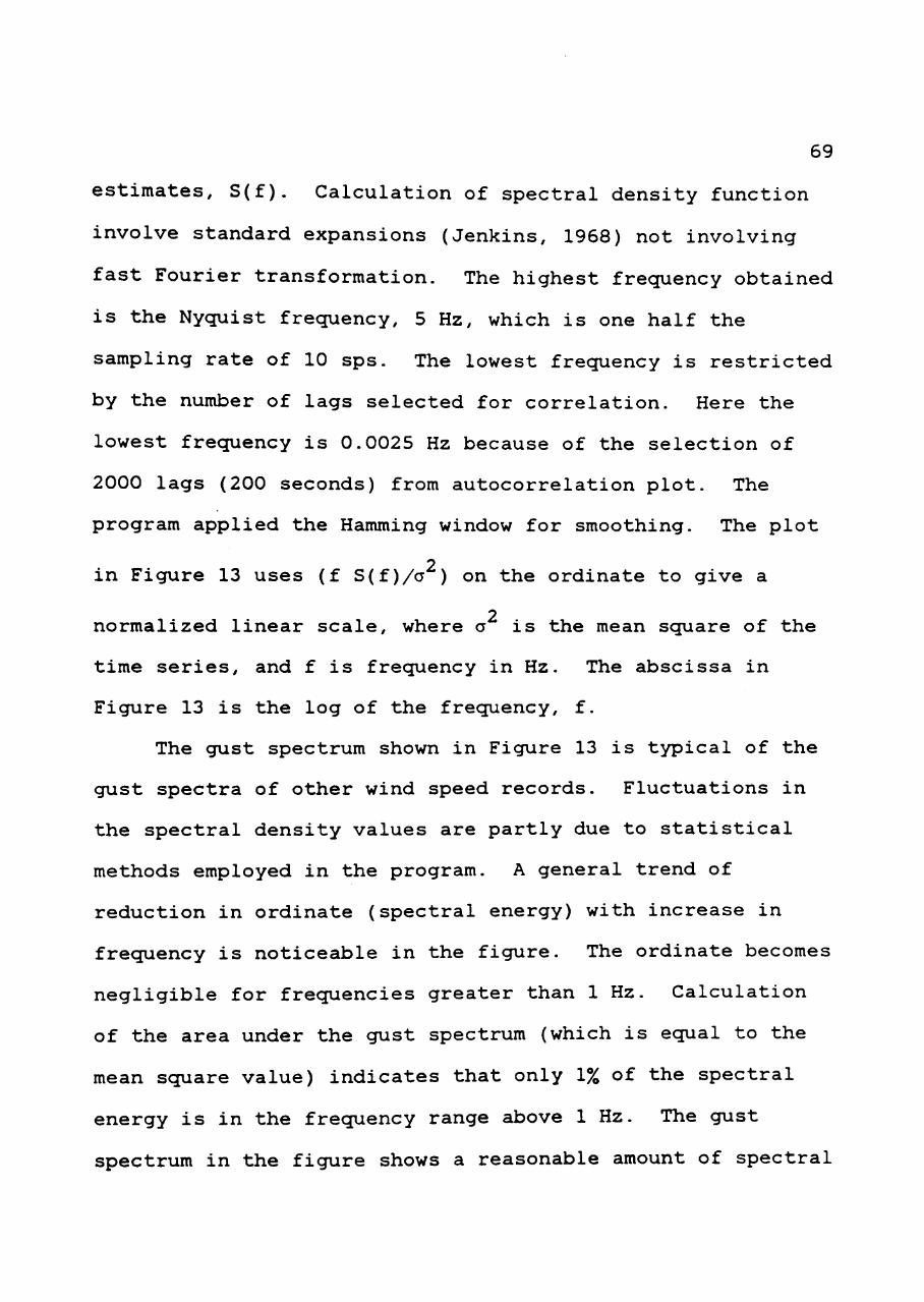
69
estimates, S(f). Calculation of spectral density function
involve standard expansions (Jenkins, 1968) not involving
fast Fourier transformation. The highest frecjuency obtained
is the Nycjuist frecjuency, 5 Hz, which is one half the
sampling rate of 10 sps. The lowest frecjuency is restricted
by the number of lags selected for correlation. Here the
lowest frecjuency is 0.0025 Hz because of the selection of
2000 lags (200 seconds) from autocorrelation plot. The
program applied the Hamming window for smoothing. The plot
2 in Figure 13 uses (f S(f)/a ) on the ordinate to give a
2 normalized linear scale, where a is the mean scjuare of the
time series, and f is frecjuency in Hz. The abscissa in
Figure 13 is the log of the frecjuency, f.
The gust spectrum shown in Figure 13 is typical of the
gust spectra of other wind speed records. Fluctuations in
the spectral density values are partly due to statistical
methods employed in the program. A general trend of
reduction in ordinate (spectral energy) with increase in
frecjuency is noticeable in the figure. The ordinate becomes
negligible for frecjuencies greater than 1 Hz. Calculation
of the area under the gust spectrum (which is ecjual to the
mean scjuare value) indicates that only 1% of the spectral
energy is in the frecjuency range above 1 Hz. The gust
spectrum in the figure shows a reasonable amount of spectral
70
o 00
O C/1
CO • U.
u 3 rt
> ^^ C3 ^ o 1) Q .
CO
O P^
o
o CO
o
o in
a
LJ 3 *
. o
o en o
o CM
, o
a
o
o o
C . O O l
S (f) - spectral density value at f f - frequency SIGSQ - mean square value
Frequency (Hertz)
Figure 13: Gust Spectrum Plot for Record NOl Recorded at 34.7 m on Tower 16/4
energy in the frequency range of 0.1 to 0.4 Hz; natural
frecjuencies of the conductors are in this range.
The analytical procedure to predict response of the
conductor developed by Davenport (1980) utilizes an
analytical form of the gust spectrum. The specific
71
analytical form used in the procedure is the one proposed by
Kaimal, as described in Chapter II (ecjuation 2.22). Gust
spectra obtained from the field data are used to determine
Kaimal's gust spectrum constants A and n. Constants A and n
represents the amplitude and slope of the analytical gust
spectrum.
The curvilinear regression procedure (Miller, 1977) is
used to obtain suitable values for constants A and n from
the field wind data. Ecjuation 2.22 is rewritten to separate
dependent and independent variables:
A u^ f h '^. (4.2)
Ecjuation 4.2 is nonlinear. It is made linear by taking
natural logarithms on both sides.
In S^(f) = ln(A nl)+n ln(^)-(n+l) ln(f). (4.3)
Ecjuation 4.3 can be written in the form
Y = C - (n+1) X (4.4)
where
C = ln(Au2) ^ ^ ln(-^), and
X = ln(f).
72
In equat ion 4 .4 , Y i s dependent on X. To solve for A
and n, normal ecjuations of t h i s ecjuation are u t i l i z e d
(Mi l l e r ,1977) . The normal equat ions a re ,
^Y = N C - (n+1) j ; x (4.5)
^X Y = C (£X) - (n+1) p 2 ^4 gj
where N = total number of data points.
Values of n and C are found by solving ecjuations 4.5
and 4.6. Substitution of n and C in ecjuation 4.3 gives the
value for A for each record. Table 7 shows the calculated A
and n values considering gust spectrum values between the
frecjuencies of (—'—- ) and 1 Hz. As indicated in Chapter h
I I , ecjuation 2.22 i s v a l i d for f g rea t e r than ( f^ ^ ) . The
h
gust spectrum values for frecjuencies greater than 1 Hz are
neglected because spectral energy (the ordinate of the gust
spectrum) is very small. The value of cionstant A is least
affected by the selection of maximum frecjuency range,
specially beyond 1 Hz. Values of constant A range between
0.005 and 0.591 (refer to Table 7). The gust spectrum (see
Figure 13) shows that the slope of the spectrum curve decreases between 0.1 and 1 Hz, and remains almost constant
beyond 1 Hz. Hence, n values are sensitive to the maximum
73
frequency range selected. Values of n range between 1.200
and 2.052.
The suggested range of values for A and n are 0.15-0.60
and 0.33-0.67, respectively (GAI, 1981). Field measured
values of A are generally within the suggested range.
However, field measured n values are much higher than the
suggested range. The parametric study of the Davenport
model for gust response factor of transmission line
structures conducted by (Twu, 1983) showed that the response
is not sensitive to the value of n.
Kaimal's analytical form of the gust spectrum (ecjuation
2.22) is valid for values of f greater than (-^LLL_Y.). For
h
the field measured data obtained at 34.7 m, this low end of
frecjuency f would be 0.3 Hz, if the mean wind speed were 20
mps. Since the conductor natural frecjuencies are in the
range of 0.1 to 0.4 Hz, near or below the low end of this
frecjuency range, Kaimal's gust spectrum constants obtained
from the field data are not appropriate for use in obtaining
response. For this reason, values of A and n of 0.3 and
0.67, respectively, as suggested by Davenport, are used to
predict the response utilizing the analytical procedure in
the next chapter.
74
Validity of Conductor Response Data
The conductor response data comprise measurements from
the transverse and longitudinal swing angle indicators and
load cell transducers. These instruments were placed at the
attachment of the insulator to the Tower 16/4 (see Figure
8). The conductors are suspended at the bottoms of the
insulators. The load cells measure axial load in the
insulator and the swing angle indicators measure swing of
the insulator from the vertical. Appropriate combinations
of values of load cells and swing angle indicators provide
vertical, longitudinal and transverse components of loads
applied on the insulators by the conductors. Interest in
this study is restricted to transverse load components since
the primary influence of wind is in the transverse
direction. The transverse load component at any instant is
calculated by the following ecjuation:
F = P cos (p sin G (4.7)
where P = axial load measured by the load cell,
(p = longitudinal swing angle, and
9 = transverse swing angle.
Twenty-one records of response for each west, east, and
central twin conductor are available. Record N14 is used as
a reference zero wind speed record to initialize all
75
records. Static loads are transferred from the conductors
to the tower structure even before being subjected to wind
loads. These initial static loads are due to the self
weight of the conductors and the inclined orientation of the
insulators. The inclined orientation of the insulators is
caused by the differences in elevation of the supporting
tower structures and by the different configuration of the
tower (refer to Chapter III). Load cell and swing angle
readings of record N14 give the weight of the conductors and
initial transverse loads. These initial transverse loads
are subtracted from the transverse loads obtained in each
record. Initialization with the zero wind speed record is
necessary to obtain conductor response due to wind only.
A time history plot of the response of the west
conductor for record NOl is shown in Figure 14. Similar to
wind records, each response record has 7200 points, which
corresponds to data collection at the rate of 10 sps for a
time duration of 12 minutes. The time history plot in
Figure 14 uses averages of 10 consecutive points; thus the
points are at one second intervals. Mean, standard
deviation and one second interval peak values are shown on
the time history plot. The purpose of these plots is to
provide a graphical display of conductor response versus
time, thereby illustrating the overall quality and trends in
the data.
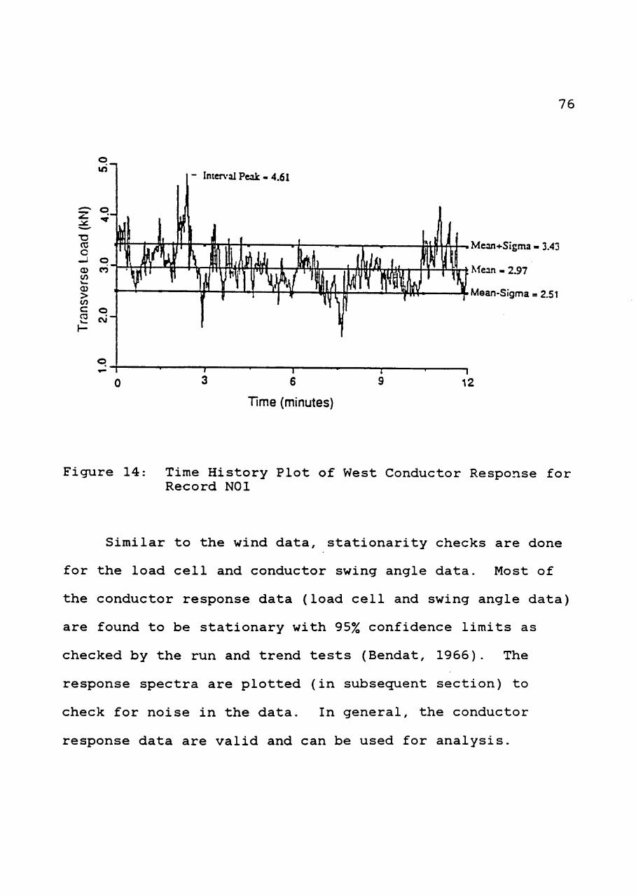
76
- Imer\-al Peak - 4.61
Time (minutes)
-, Mean+Sigma » 3.43
Mean - 2.97
Mean-Sigma = 2.51
Figure 14: Time History Plot of West Conductor Response for Record NOl
Similar to the wind data, stationarity checks are done
for the load cell and conductor swing angle data. Most of
the conductor response data (load cell and swing angle data)
are found to be stationary with 95% confidence limits as
checked by the run and trend tests (Bendat, 1966). The
response spectra are plotted (in subsecjuent section) to
check for noise in the data. In general, the conductor
response data are valid and can be used for analysis.
77
The mean and RMS values of response for the three
conductors (west, east, and central) are shown in Table 9.
The negative values in Table 9 indicate wind from the east.
The choice of sign for conductor response is arbitrary. The
values in the table show that response recorded at the
central conductor is higher than that for the west and east
conductors. This is expected since the central conductor is
suspended at 26.7 m above ground level, which is 8.4 m above
the west and east conductors at Tower 16/4 (see Figure 8).
The response of the west conductor is slightly higher
than that of the east conductor in many records, even though
they are suspended at the same height above ground. The
range of the difference in values is from -0.08 to 0.33 kN;
less than 10% of the recorded values. There could be one of
several reasons or a combination of reasons for this
difference. These reasons and observations based on the
data are given below.
One set of twin conductors (west or east) could shield
or intensify wind load effect on the other set of twin
conductors. This is not likely because the west and east
conductors are 13.4 m apart at Tower 16/4. In addition,
data do not show a specific trend in response for winds
coming from east or west.
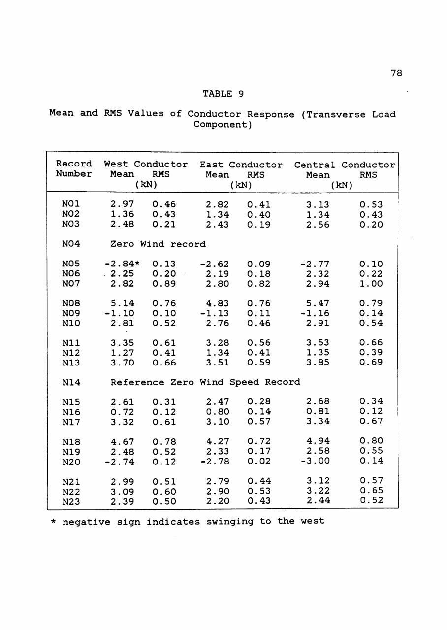
78
TABLE 9
Mean and RMS Values of Conductor Response (Transverse Load Component)
Record Number
NOl N02 N03
N04
N05 NO 6 N07
NOB N09 NIO
Nil N12 N13
N14
N15 N16 N17
N18 N19 N20
N21 N22 N23
West Conductor Mean RMS
(kN)
2.97 1.36 2.48
Zero
-2.84* 2.25 2.82
5.14 -1.10 2.81
3.35 1.27 3.70
0.46 0.43 0.21
Wind reco
0.13 0.20 0.89
0.76 0.10 0.52
0.61 0.41 0.66
Reference Zero
2.61 0.72 3.32
4.67 2.48 -2.74
2.99 3.09 2.39
0.31 0.12 0.61
0.78 0.52 0.12
0.51 0.60 0.50
East Conductor Mean RMS
(kN)
2.82 1.34 2.43
rd
-2.62 2.19 2.80
4.83 -1.13 2.76
3.28 1.34 3.51
0.41 0.40 0.19
0.09 0.18 0.82
0.76 0.11 0.46
0.56 0.41 0.59
Wind Speed Recc
2.47 0.80 3.10
4.27 2.33 -2.78
2.79 2.90 2.20
0.28 0.14 0.57
0.72 0.17 0.02
0.44 0.53 0.43
Central Conductor Mean
(kN)
3.13 1.34 2.56
-2.77 2.32 2.94
5.47 -1.16 2.91
3.53 1.35 3.85
>rd
2.68 0.81 3.34
4.94 2.58 -3.00
3.12 3.22 2.44
RMS
0.53 0.43 0.20
0.10 0.22 1.00
0.79 0.14 0.54
0.66 0.39 0.69
0.34 0.12 0.67
0.80 0.55 0.14
0.57 0.65 0.52
* negative sign indicates swinging to the west
79
Measurement of weight of the conductor during reference
zero wind condition can cause discrepancy in calculation of
transverse loads. The west conductor weight is recorded
higher than the east conductor by 2.4 kN (a difference of
9%). The information obtained from the field indicates that
detuner dampers are added to the west conductors. These
dampers account for approximately 0.9 kN of extra weight.
Discrepancy in dead weight of 1.5 kN in west conductor is
not reconciled. This extra dead weight could be a reason
for higher response of west conductor compared to east
conductor in most of the records (see Table 9).
Accuracy in swing angle measurements is important for
estimation of the transverse load component. The swing
angle indicators have a resolution of 0.2 degrees.
Discrepancy in swing angle reading of 0.2 degree could cause
error in response by 2-4% for the range of readings obtained
in these data. Accuracy of the swing angle indicator can be
one of the factors causing a difference in recorded
response. Notwithstanding the differences in recorded
responses of conductors mentioned above, the data for the
three conductors are fairly consistent. Some variations and
scattering in the field data are inherent; they cannot be
avoided. In general, conductor response data are considered
valid for use in analysis.
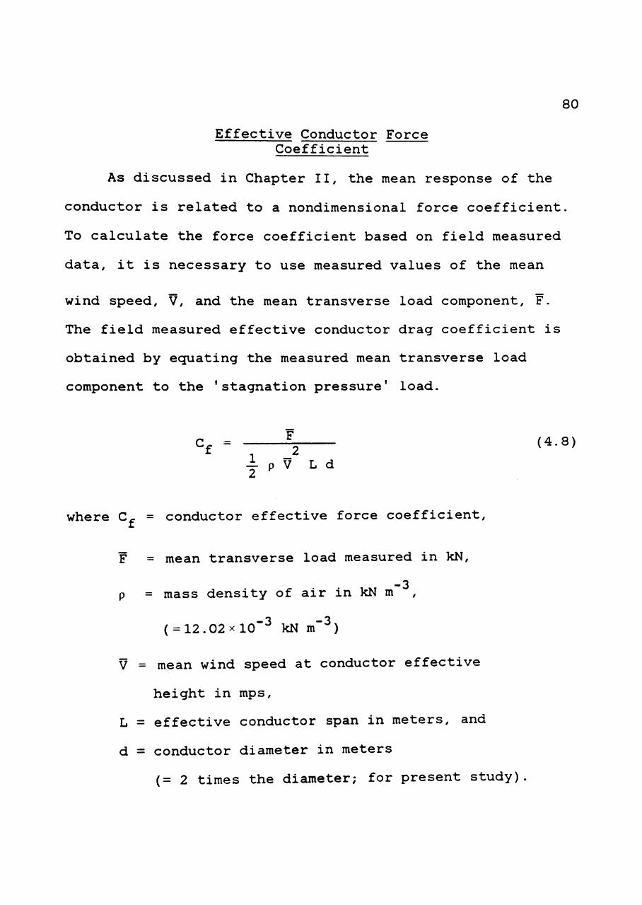
80
Effective Conductor Force Coefficient
As discussed in Chapter II, the mean response of the
conductor is related to a nondimensional force coefficient.
To calculate the force coefficient based on field measured
data, it is necessary to use measured values of the mean
wind speed, V, and the mean transverse load component, F.
The field measured effective conductor drag coefficient is
obtained by ecjuating the measured mean transverse load
component to the 'stagnation pressure' load.
4 p V L d 2
where C^ = conductor effective force coefficient,
F = mean transverse load measured in kN,
-3 p = mass density of air in kN m
( = 12.02x10"^ kN m"^)
V = mean wind speed at conductor effective
height in mps,
L = effective conductor span in meters, and
d = conductor diameter in meters
(= 2 times the diameter; for present study)
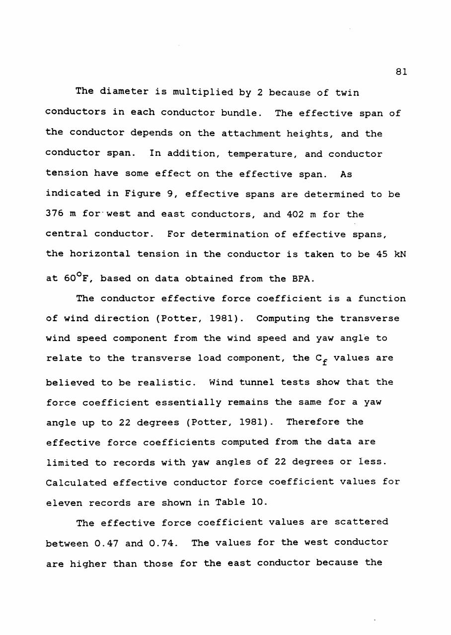
81
The diameter is multiplied by 2 because of twin
conductors in each conductor bundle. The effective span of
the conductor depends on the attachment heights, and the
conductor span. In addition, temperature, and conductor
tension have some effect on the effective span. As
indicated in Figure 9, effective spans are determined to be
376 m for west and east conductors, and 402 m for the
central conductor. For determination of effective spans,
the horizontal tension in the conductor is taken to be 45 kN
at 60 F, based on data obtained from the BPA.
The conductor effective force coefficient is a function
of wind direction (Potter, 1981). Computing the transverse
wind speed component from the wind speed and yaw angle to
relate to the transverse load component, the C^ values are
believed to be realistic. Wind tunnel tests show that the
force coefficient essentially remains the same for a yaw
angle up to 22 degrees (Potter, 1981). Therefore the
effective force coefficients computed from the data are
limited to records with yaw angles of 22 degrees or less.
Calculated effective conductor force coefficient values for
eleven records are shown in Table 10.
The effective force coefficient values are scattered
between 0.47 and 0.74. The values for the west conductor
are higher than those for the east conductor because the
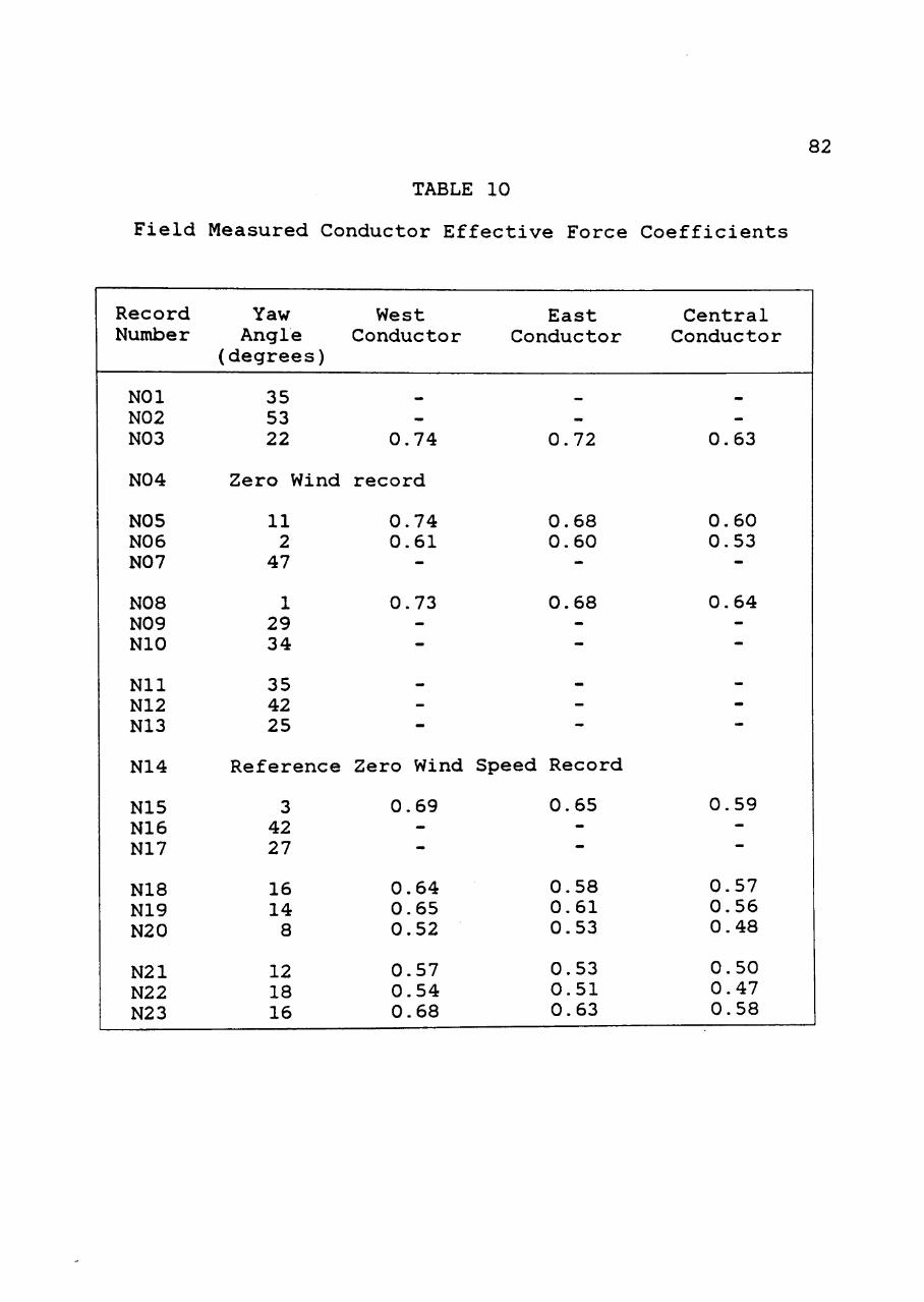
82
TABLE 10
Field Measured Conductor Effective Force Coefficients
Record Yaw West East Central Number Angle Conductor Conductor Conductor
(degrees)
NOl 35 -N02 53 -N03 22 0.74 0.72 0.63
N04 Zero Wind record
N05 NO 6 N07
NOB N09 NIO
Nil N12 N13
11 2 47
1 29 34
35 42 25
0 0
0
.74
.61 -
.73 -
-
•
-
-
0.68 0.60
-
0.68 -
-
—
-
-
0.60 0.53
-
0.64 -
—
-
-
-
N14 Reference Zero Wind Speed Record
N15 3 0.69 0.65 0.59 N16 42 -N17 27 -
N18 16 0.64 0.58 0.57 N19 14 0.65 0.61 0.56 N20 8 0.52 0.53 0.48
N21 12 0.57 N22 18 0.54 N23 16 0.68
0.53 0.51 0.63
0.50 0.47 0.58
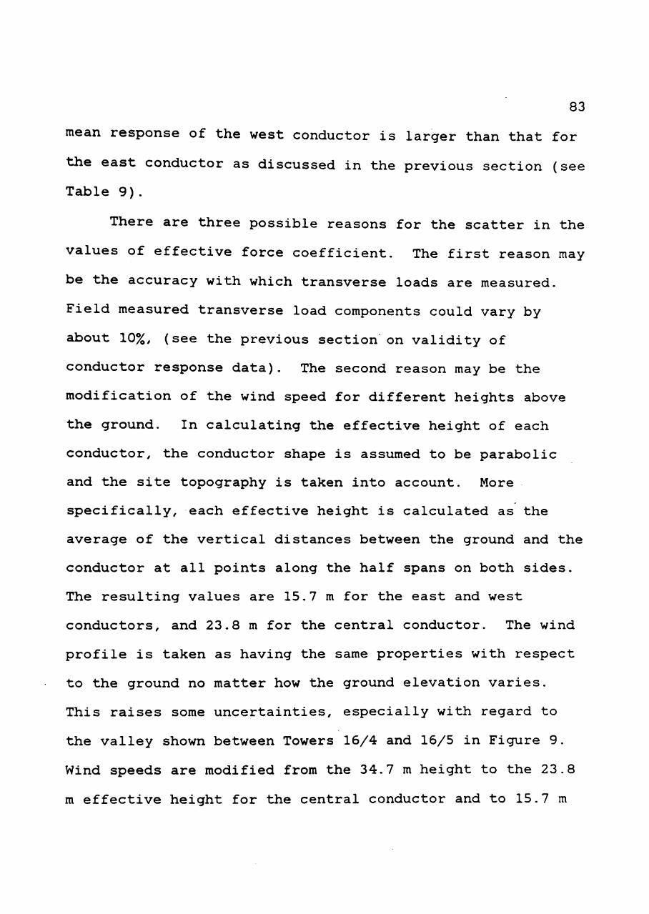
83
mean response of the west conductor is larger than that for
the east conductor as discussed in the previous section (see
Table 9).
There are three possible reasons for the scatter in the
values of effective force coefficient. The first reason may
be the accuracy with which transverse loads are measured.
Field measured transverse load components could vary by
about 10%, (see the previous section on validity of
conductor response data). The second reason may be the
modification of the wind speed for different heights above
the ground. In calculating the effective height of each
conductor, the conductor shape is assumed to be parabolic
and the site topography is taken into account. More
specifically, each effective height is calculated as the
average of the vertical distances between the ground and the
conductor at all points along the half spans on both sides.
The resulting values are 15.7 m for the east and west
conductors, and 23.8 m for the central conductor. The wind
profile is taken as having the same properties with respect
to the ground no matter how the ground elevation varies.
This raises some uncertainties, especially with regard to
the valley shown between Towers 16/4 and 16/5 in Figure 9.
Wind speeds are modified from the 34.7 m height to the 23.8
m effective height for the central conductor and to 15.7 m
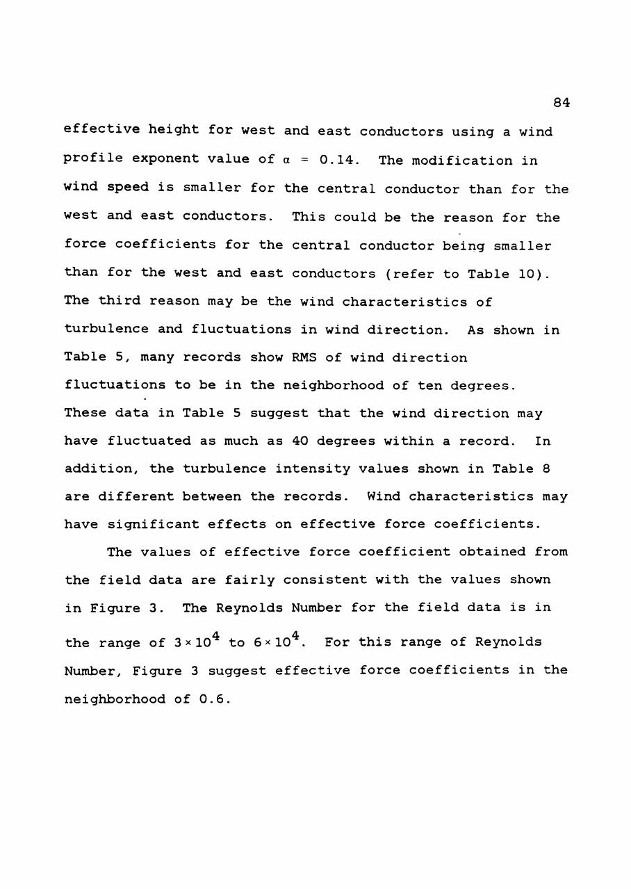
84
effective height for west and east conductors using a wind
profile exponent value of a = 0.14. The modification in
wind speed is smaller for the central conductor than for the
west and east conductors. This could be the reason for the
force coefficients for the central conductor being smaller
than for the west and east conductors (refer to Table 10).
The third reason may be the wind characteristics of
turbulence and fluctuations in wind direction. As shown in
Table 5, many records show RMS of wind direction
fluctuations to be in the neighborhood of ten degrees.
These data in Table 5 suggest that the wind direction may
have fluctuated as much as 40 degrees within a record. In
addition, the turbulence intensity values shown in Table 8
are different between the records. Wind characteristics may
have significant effects on effective force coefficients.
The values of effective force coefficient obtained from
the field data are fairly consistent with the values shown
in Figure 3. The Reynolds Number for the field data is in
4 4 the range of 3x10 to 6x10 . For this range of Reynolds Number, Figure 3 suggest effective force coefficients in the
neighborhood of 0.6.
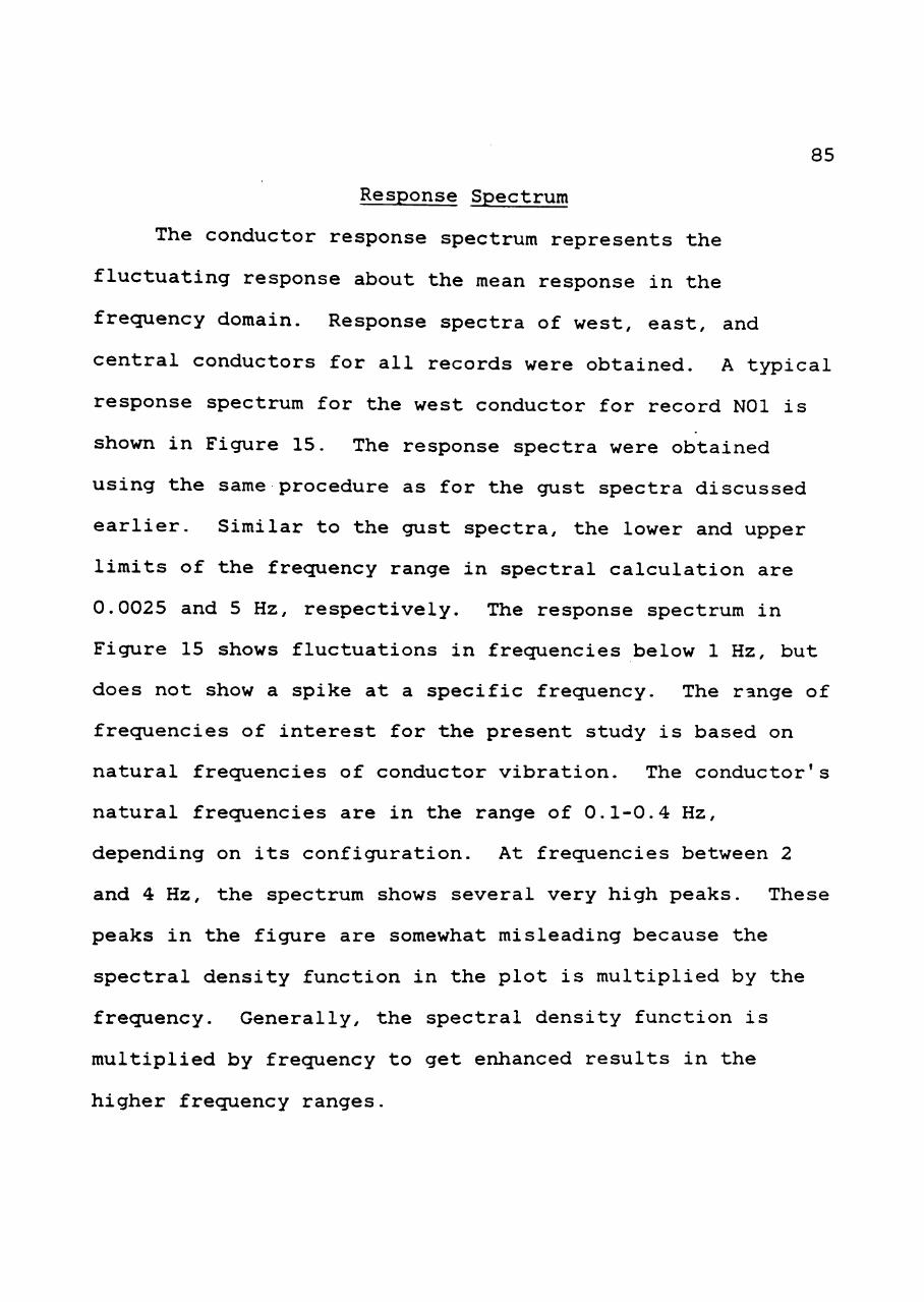
85
Response Spectrum
The conductor response spectrum represents the
fluctuating response about the mean response in the
frecjuency domain. Response spectra of west, east, and
central conductors for all records were obtained. A typical
response spectrum for the west conductor for record NOl is
shown in Figure 15. The response spectra were obtained
using the same procedure as for the gust spectra discussed
earlier. Similar to the gust spectra, the lower and upper
limits of the frecjuency range in spectral calculation are
0.0025 and 5 Hz, respectively. The response spectrum in
Figure 15 shows fluctuations in frecjuencies below 1 Hz, but
does not show a spike at a specific frecjuency. The range of
frecjuencies of interest for the present study is based on
natural frecjuencies of conductor vibration. The conductor's
natural frecjuencies are in the range of 0.1-0.4 Hz,
depending on its configuration. At frecjuencies between 2
and 4 Hz, the spectrum shows several very high peaks. These
peaks in the figure are somewhat misleading because the
spectral density function in the plot is multiplied by the
frecjuency. Generally, the spectral density function is
multiplied by frecjuency to get enhanced results in the
higher frecjuency ranges.
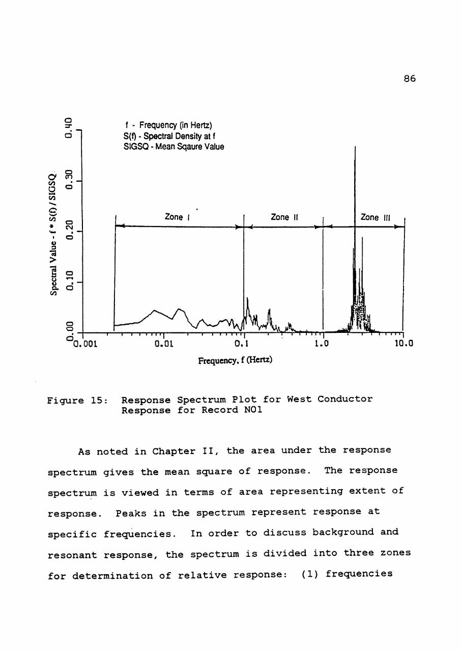
86
a CO O teiH
CO " » O >»,' CO
« V M
1
O 3 •3 >
1 ii CU
CO
Q 3 *
a
n CD
• a
o CM
• O
o .—1
f
o
a o
G.OOL
f - Frequency (in Hertz) S(f) - Spectral Density at f SIGSQ - Mean Sqaure Value
Zone Zone
^^Vr-n.. O . l
Frequenc:y, f (Hertz)
l . O
Zone III
Figure 15: Response Spectrum Plot for West Conductor Response for Record NOl
As noted in Chapter II, the area under the response
spectrum gives the mean scjuare of response. The response
spectrum is viewed in terms of area representing extent of
response. Peaks in the spectrum represent response at
specific frecjuencies. In order to discuss background and
resonant response, the spectrum is divided into three zones
for determination of relative response: (1) frequencies
87
less than 0.1 Hz, (2) frequencies between 0.1 Hz and 1.0 Hz,
and (3) frequencies greater than 1 Hz. Each zone of the
spectrum is reviewed in light of the conductor response to
wind.
The spectral area in the zone of frecjuencies less than
0.1 Hz is in the neighborhood of 75% for all records. This
response is primarily due to the background turbulence where
wind has significant turbulent energy (see Figure 13). The
peaks in the spectra in this zone do not represent dynamic
amplification of the response.
The spectral area in the zone between frecjuencies of
0.1 and 1.0 Hz is close to 15% for all records. Fundamental
transverse frecjuency of the conductor, f , in Hz for a
parabolic profile can be obtained using ecjuation 2.27. The
conductor sag depends on conductor span, horizontal tension
and temperature. The conductor span on the south side of
the Tower 16/4 is 450 m and toward the north it is 252 m
(see Figure 9). The sags, calculated using conductor
horizontal tension of 45 kN at 60°F, are 6.3 m and 21.0 m
corresponding to the 252 m and 450 m spans, respectively (a
parabolic profile is assumed). Using ecjuation 2.27 with
estimated sags, the calculated natural frecjuencies in the
transverse direction are 0.12 Hz and 0.22 Hz. The spectrum
in Figure 15 shows small but distinguishable peaks in the
88
neighborhood of these frequencies. The two unequal spans
are expected to respond in the transverse direction
independent of each other due to the low stiffness of the
conductor. The two peaks are judged to be due to resonant
response at natural transverse frecjuencies of the conductor.
At frecjuencies close to the conductor natural
frecjuencies the gust spectrum in Figure 13 shows that wind
has a fair amount of energy. Presence of gust energy at
natural frecjuencies of the conductor can cause significant
resonant amplification of the conductor response.
The spectral areas in the zone of frecjuencies greater
than 1 Hz are less than 15% in most of the records. High
spectral peaks (Figure 15) in the 2-4 Hz frecjuency range are
believed to be due to vibration of the tower and the
frecjuency of the swing angle indicators. These frecjuencies
of the tower and instruments enter into the conductor
response records since the conductor is connected to the
tower through load cells and swing angle indicators.
Natural frequencies of Tower 16/4 are determined using
MSC/NASTRAN version 63 software. The tower structure is
modelled as a space frame, without conductors and overhead
ground wires. Natural frecjuencies of the tower are 2.88,
3.01 and 4.92 Hz, corresponding to longitudinal, transverse,
and torsional modes of vibration, respectively. In
89
addition, the frequency of vibration of the swing angle
indicator is 3.2 Hz (Kempner, 1980). These frecjuencies of
the tower and the swing angle indicator are believed to
cause high peaks in the response spectrum in the frecjuency
range of 2 to 4 Hz. Even though spectral peaks are high in
the frecjuency range above 1 Hz, the amount of energy is
relatively low.
Since the amount of gust spectral energy above 1 Hz in
Figure 13 is very small and since peaks in the response
spectra can be justified as above, it is believed that the
response spectral energy in the frecjuency range above 1 Hz
is not due to response of the conductor to wind. This
spectral energy is neglected in further consideration of the
response of the conductors. The background and resonant
responses assessed from the response spectra are compared
with the analytical procedure in the next chapter.
CHAPTER V
COMPARISON AND REFINEMENT OF THE
ANALYTICAL MODEL
The goal of the present study is to compare and to
refine the analytical model using the results of field data.
The analytical model proposed by Davenport (1980) to
determine peak response of transmission line structures was
presented in Chapter II. The key elements in determining
the fluctuating response of conductors in the model are the
background response and the resonant response (see ecjuation
2.23). In addition, the model recjuires establishment a
value for the peak factor to determine peak response (see
ecjuation 2.1).
The field data analysis yields the peak response as
well as the fluctuating response. Background and resonant
responses are determined from response spectra of field data
utilizing the procedure indicated in Chapter IV. Peak
factors are obtained from the field peak responses utilizing
the upcrossing rate procedure.
Background and resonant responses assessed from the
field data are compared with values calculated using the
analytical model. Joint acceptance function coefficients
90
91
are obtained from the field data to refine the background
response of the analytical model. Also, aerodynamic damping
ratios are recovered from the field data to improve the
resonant response of the analytical model. Since the
fluctuating response depends on many parameters, total
fluctuating responses from field data are not compared with
total fluctuating response predicted using the Davenport
model (1980).
Comparison of Analytically Predicted Mean Square Response With Field
Measured Values
One of the two parts of the fluctuating response
component in ecjuation 2.1 is the mean scjuare value. In the
frecjuency domain analysis, the mean scjuare value of response
is computed as the area under the response spectrum. The
mean scjuare value can be considered as a summation of
background response, B , and resonant response, R (ecjuation
2.23). Background response is due to the wind turbulence at
low frecjuencies, and can be considered as quasi-static
response. Resonant response is due to coincidence of
conductor natural frecjuencies with gust frecjuencies. This
resonant response is the area under the response spectrum at
frecjuencies close to conductor natural frecjuencies.
92
Field Measured Mean Scjuare Response
The gust spectrum of Figure 13 shows that the wind
turbulence has energy up to 1 Hz, and energy beyond 1 Hz is
negligible. Conductor natural frecjuencies are in the range
of 0.1 to 0.4 Hz, hence the resonant peaks should dominate
above the background response in this frecjuency range. It
is difficult to separate background and resonant responses
in the field data. In Figure 16, which is the same response
spectrum as Figure 15, there are peaks at the natural
frecjuencies of the conductors: 0.12 and 0.22 Hz. However,
these peaks are diffused. As discussed in Chapter IV, the
spectral areas between the frecjuencies of 0.1 and 1.0 Hz for
most records were less than 15% of the total area under the
response spectrum (total mean scjuare value). At the risk of
being on the high side, the total spectral areas between
frecjuencies of 0.1 and 1.0 Hz are assumed to be resonant
response. The error introduced by this assumption is small
because the response in this frecjuency range is a small
portion of the total fluctuating response. This resonant
response is indicated by R in Figure 16.
It is reasonable to assume that the area under the
response spectrum below 0.1 Hz is the background response.
This area is close to 75% of the total area (total mean
scjuare value) in most of the records as discussed in Chapter
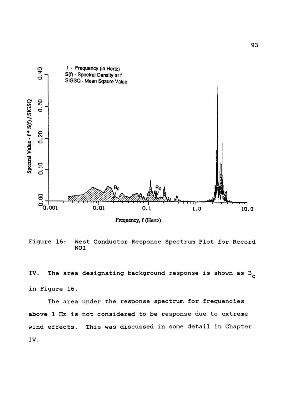
93
a 3* CJ
o en a
CO
O d CO
CO
«M CM
u o a •a > 1 a ° CO o
Q.OOL
f - Frequency (in Hertz) S(f) - Spectral Density at f SIGSQ - Mean Sqaure Value
0.1
Frequency, f (Hertz)
10.0
Figure 16: West Conductor Response Spectrum Plot for Record NOl
IV. The area designating background response is shown as B
in Figure 16.
The area under the response spectrum for frecjuencies
above 1 Hz is not considered to be response due to extreme
wind effects. This was discussed in some detail in Chapter
IV
94
Delineation of background and resonant responses in the
field response spectra permits assessment of responses in
each of the three conductors, west, east, and central
conductors, for all twenty-one field records. Field
measured values for background and resonant responses for
west, east, and central conductors are tabulated in Tables
11 through 13, along with mean scjuare values, for each
conductor. These values are compared with values predicted
by the analytical model as described in the next section.
The mean scjuare values of the three conductors are
fairly consistent, but have scatter for a given record.
This is not surprising, since there was variation (by about
10%) in the mean response of the three conductors (refer to
Table 9). It is reasonable to expect larger variation in
fluctuating response between the conductors. The variation
in the field data suggests that results will have scatter,
and that it is important to use an ensemble of data for
appropriate interpretation of the results.
Analytical Model Predicted Mean Scjuare Value
The analytical model used to predict the background and
resonant response contains a number of wind and conductor
related parameters (see ecjuations 2.24 and 2.25). These
parameters can be separated into fixed and variable
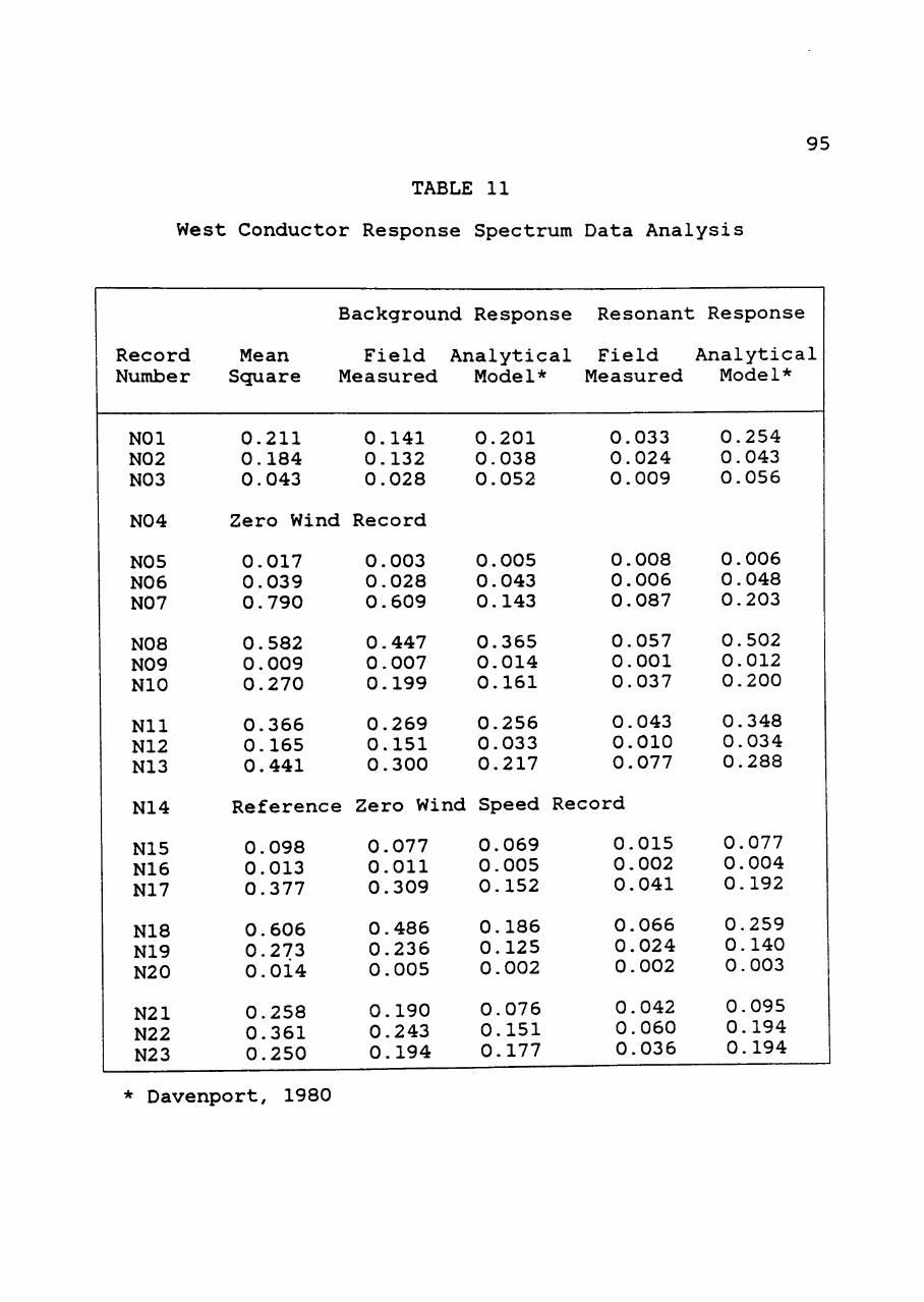
95
TABLE 11
West Conductor Response Spectrum Data Analysis
Record Number
NOl N02 N03
N04
N05 NO 6 N07
2 2
2 M
OO
O
vD
00
Nil N12 N13
N14
N15 N16 N17
N18 N19 N20
2 2
2 to
to
to
CA
) to
M
Mean Scjuare
0.211 0.184 0.043
Background Response
Field Analytical Measured Model*
0.141 0.132 0.028
Zero Wind Record
0.017 0.039 0.790
0.582 0.009 0.270
0.366 0.165 0.441
0.003 0.028 0.609
0.447 0.007 0.199
0.269 0.151 0.300
Reference Zero Wind
0.098 0.013 0.377
0.606 0.273 0.014
0.258 0.361 0.250
0.077 0.011 0.309
0.486 0.236 0.005
0.190 0.243 0.194
0.201 0.038 0.052
0.005 0.043 0.143
0.365 0.014 0.161
0.256 0.033 0.217
Resonant
Field Measured
0.033 0.024 0.009
0.008 0.006 0.087
0.057 0.001 0.037
0.043 0.010 0.077
Speed Record
0.069 0.005 0.152
0.186 0.125 0.002
0.076 0.151 0.177
0.015 0.002 0.041
0.066 0.024 0.002
0.042 0.060 0.036
. Response
Analytical Model*
0.254 0.043 0.056
0.006 0.048 0.203
0.502 0.012 0.200
0.348 0.034 0.288
0.077 0.004 0.192
0.259 0.140 0.003
0.095 0.194 0.194
* Davenport, 1980
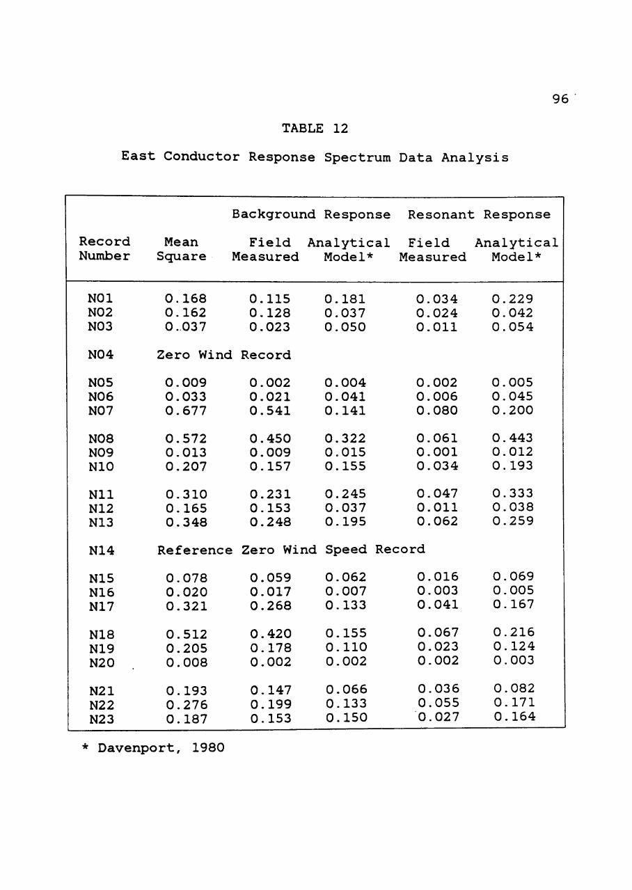
96
TABLE 12
East Conductor Response Spectrum Data Analysis
Record Number
rH
CM
C
O
o o
o
2 2 2
N04
N05 NO 6 N07
2 2
2 M
OO
O
vD
00
Nil N12 N13
N14
N15 N16 N17
2 2
2 to
M M
O
VD
00
2 2
2 to
to
to
CA)
to M
Mean Scjuare
0.168 0.162 0.037
Background Response
Field Analytical Measured Model*
0.115 0.128 0.023
Zero Wind Record
0.009 0.033 0.677
0.572 0.013 0.207
0.310 0.165 0.348
0.002 0.021 0.541
0.450 0.009 0.157
0.231 0.153 0.248
Reference Zero Wind
0.078 0.020 0.321
0.512 0.205 0.008
0.193 0.276 0.187
0.059 0.017 0.268
0.420 0.178 0.002
0.147 0.199 0.153
0.181 0.037 0.050
0.004 0.041 0.141
0.322 0.015 0.155
0.245 0.037 0.195
Resonant Response
Field Measured
0.034 0.024 0.011
0.002 0.006 0.080
0.061 0.001 0.034
0.047 0.011 0.062
Speed Record
0.062 0.007 0.133
0.155 0.110 0.002
0.066 0.133 0.150
0.016 0.003 0.041
0.067 0.023 0.002
0.036 0.055 0.027
Analytical Model*
0.229 0.042 0.054
0.005 0.045 0.200
0.443 0.012 0.193
0.333 0.038 0.259
0.069 0.005 0.167
0.216 0.124 0.003
0.082 0.171 0.164
* Davenport, 1980
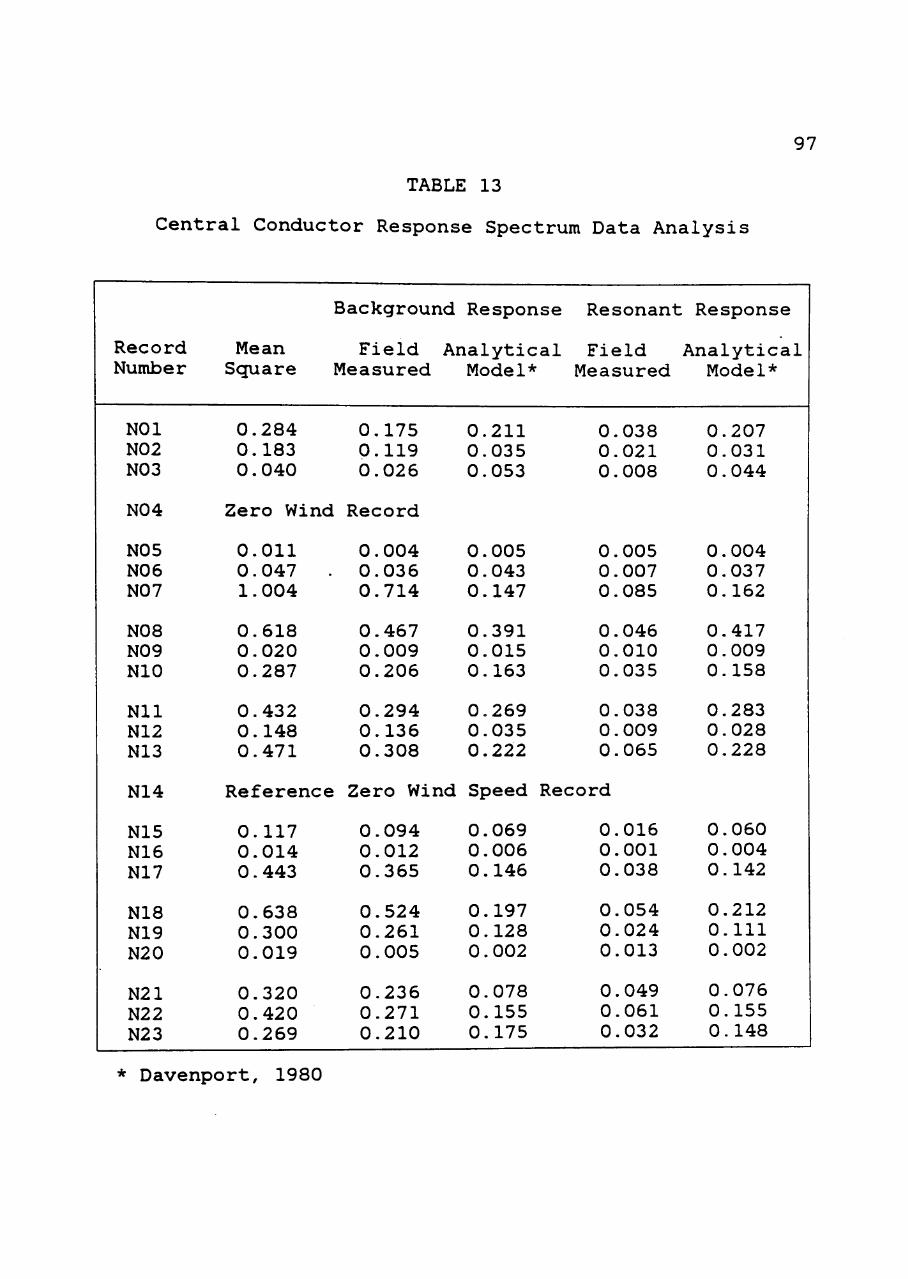
97
TABLE 13
Central Conductor Response Spectrum Data Analysis
Record Number
NOl N02 N03
NO 4
NO 5 NO 6 N07
NOB NO 9 NIO
Nil N12 N13
N14
N15 N16 N17
N18 N19 N20
N21 N22 N23
Mean Scjuare
0.284 0.183 0.040
Background Response
Field Analytical Measured
0.175 0.119 0.026
Zero Wind Record
0.011 0.047 1.004
0.618 0.020 0.287
0.432 0.148 0.471
0.004 0.036 0.714
0.467 0.009 0.206
0.294 0.136 0.308
Reference Zero Wind
0.117 0.014 0.443
0.638 0.300 0.019
0.320 0.420 0.269
0.094 0.012 0.365
0.524 0.261 0.005
0.236 0.271 0.210
Model*
0.211 0.035 0.053
0.005 0.043 0.147
0.391 0.015 0.163
0.269 0.035 0.222
Resonant
Field Measured
0.038 0.021 0.008
0.005 0.007 0.085
0.046 0.010 0.035
0.038 0.009 0.065
Speed Record
0.069 0.006 0.146
0.197 0.128 0.002
0.078 0.155 0.175
0.016 0.001 0.038
0.054 0.024 0.013
0.049 0.061 0.032
Response
Analytical Model*
0.207 0.031 0.044
0.004 0.037 0.162
0.417 0.009 0.158
0.283 0.028 0.228
0.060 0.004 0.142
0.212 0.111 0.002
0.076 0.155 0.148
* Davenport, 1980
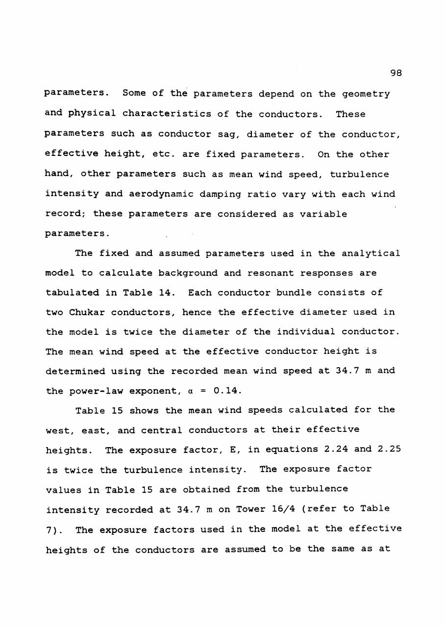
98
parameters. Some of the parameters depend on the geometry
and physical characteristics of the conductors. These
parameters such as conductor sag, diameter of the conductor,
effective height, etc. are fixed parameters. On the other
hand, other parameters such as mean wind speed, turbulence
intensity and aerodynamic damping ratio vary with each wind
record; these parameters are considered as variable
parameters.
The fixed and assumed parameters used in the analytical
model to calculate background and resonant responses are
tabulated in Table 14. Each conductor bundle consists of
two Chukar conductors, hence the effective diameter used in
the model is twice the diameter of the individual conductor.
The mean wind speed at the effective conductor height is
determined using the recorded mean wind speed at 34.7 m and
the power-law exponent, a = 0.14.
Table 15 shows the mean wind speeds calculated for the
west, east, and central conductors at their effective
heights. The exposure factor, E, in ecjuations 2.24 and 2.25
is twice the turbulence intensity. The exposure factor
values in Table 15 are obtained from the turbulence
intensity recorded at 34.7 m on Tower 16/4 (refer to Table
7). The exposure factors used in the model at the effective
heights of the conductors are assumed to be the same as at
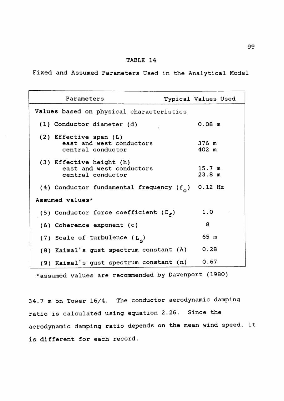
99
TABLE 14
Fixed and Assumed Parameters Used in the Analytical Model
Parameters Typical Values Used
0 . 0 8 m
376 m 402 m
15 .7 2 3 . 8
m m
Values based on physical characteristics
(1) Conductor diameter (d)
(2) Effective span (L) east and west conductors central conductor
(3) Effective height (h) east and west conductors central conductor
(4) Conductor fundamental frecjuency (f ) 0.12 Hz
Assumed values*
(5) Conductor force coefficient (C^) 1.0
(6) Coherence exponent (c) 8
(7) Scale of turbulence (L ) 65 m ^ ' s
(8) Kaimal's gust spectrum constant (A) 0.28
(9) Kaimal's gust spectrum constant (n) 0.67
*assumed values are recommended by Davenport (1980)
34.7 m on Tower 16/4. The conductor aerodynamic damping
ratio is calculated using ecjuation 2.26. Since the
aerodynamic damping ratio depends on the mean wind speed, it
is different for each record.
100
TABLE 15
Variable Parameters Used in the Analytical Model
Record Number
NOl N02 N03
N04 Ze
Exposure Factor
0.36 0.34 0.22
ro Wind Rec<
Mean
@ 15.7
16.9 14.7 13.3
ord
Wind
m*
Speed (mps)
@ 23.8 m**
17.9 15.5 14.1
N05 NO 6 NO 7
222
MOO
O v
D 00
Nil N12 N13
N14
N15 N16 N17
2 2 2
to M M
O V
D 00
2 2 2
to to to
CO to M
0.06 0.22 0.32
0.28 0.26 0.34
0.36 0.34 0.30
Reference
0.24 0.24 0.28
0.22 0.34 0.04
0.22 0.30 0.42
14.2 13.9 20.1
19.3 8.6 16.6
18.9 12.6 18.2
Zero Wind Speed Record
14.1 9.0 16.9
19.6 14.2 16.6
16.6 17.3 13.6
15.0 14.7 21.2
20.4 9.1 17.5
19.9 13.2 19.2
14.9 9.5 17.8
20.7 15.0 17.5
17.5 18.3 14.4
* effective height for west and east conductors ** effective height for central conductor
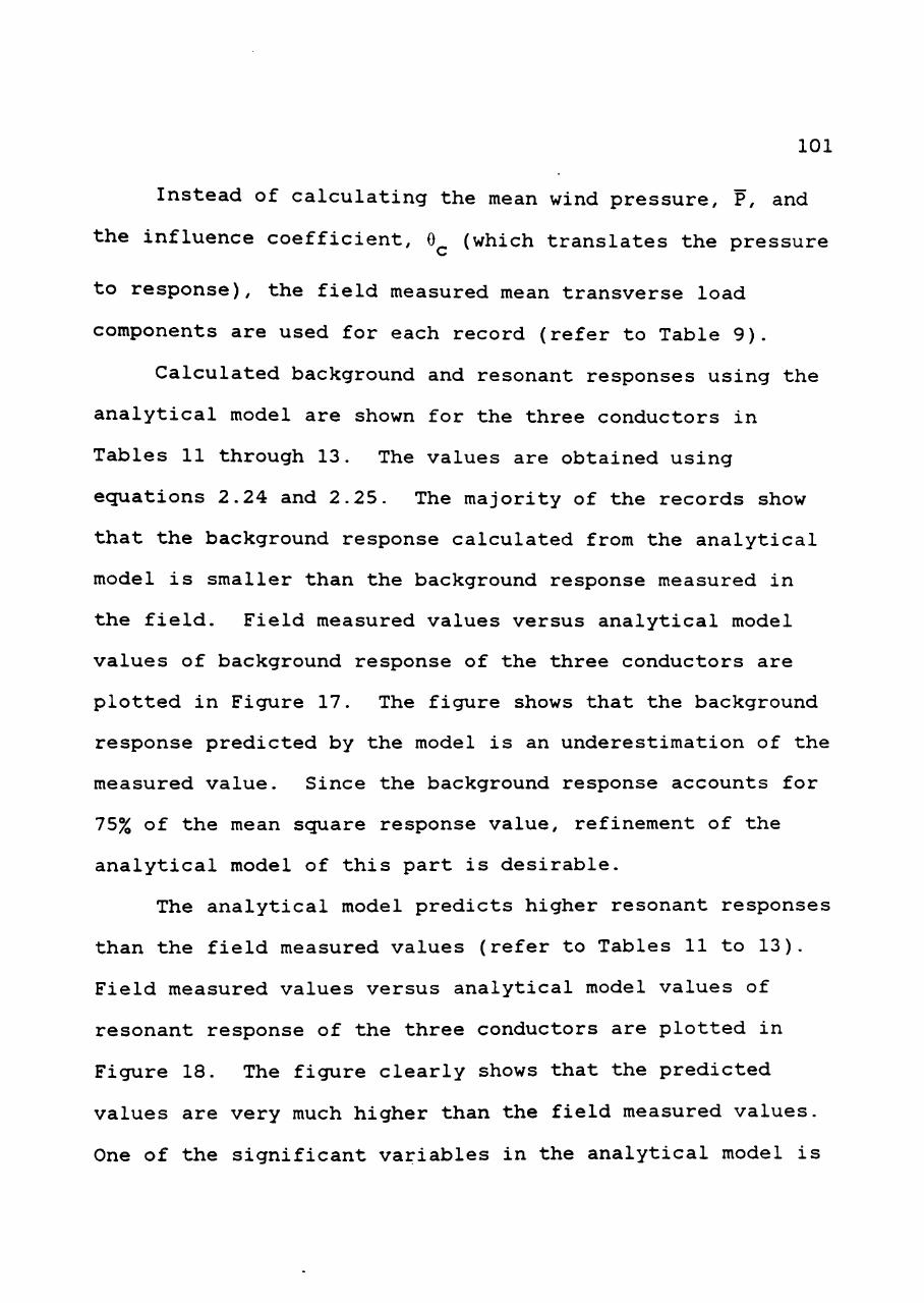
101
Instead of calculating the mean wind pressure, P, and
the influence coefficient, 0 (which translates the pressure
to response), the field measured mean transverse load
components are used for each record (refer to Table 9).
Calculated background and resonant responses using the
analytical model are shown for the three conductors in
Tables 11 through 13. The values are obtained using
ecjuations 2.24 and 2.25. The majority of the records show
that the background response calculated from the analytical
model is smaller than the background response measured in
the field. Field measured values versus analytical model
values of background response of the three conductors are
plotted in Figure 17. The figure shows that the background
response predicted by the model is an underestimation of the
measured value. Since the background response accounts for
75% of the mean scjuare response value, refinement of the
analytical model of this part is desirable.
The analytical model predicts higher resonant responses
than the field measured values (refer to Tables 11 to 13).
Field measured values versus analytical model values of
resonant response of the three conductors are plotted in
Figure 18. The figure clearly shows that the predicted
values are very much higher than the field measured values.
One of the significant variables in the analytical model is
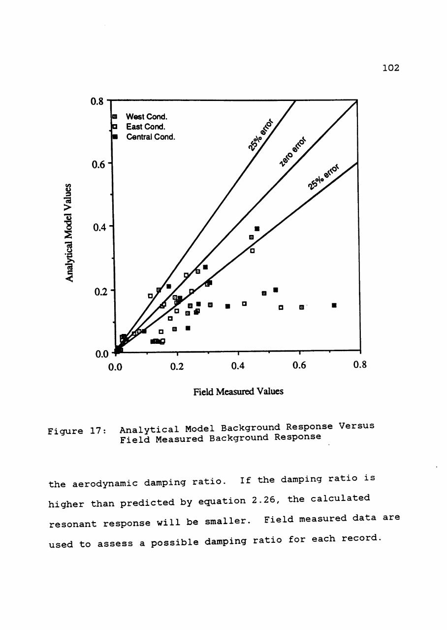
102
0.8
U
s •a >
•a
•a
o West Cond. East Cond. Central Cond
0.6-
0.4-
1 1 * r—
0.4 0.6
Field Measured Values
0.8
Figure 17: Analytical Model Background Response Versus Field Measured Background Response
the aerodynamic damping ratio. If the damping ratio is
higher than predicted by equation 2.26, the calculated
resonant response will be smaller. Field measured data are
used to assess a possible damping ratio for each record.
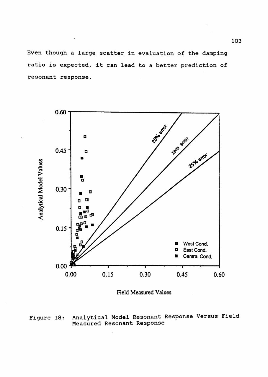
103
Even though a large scatter in evaluation of the damping
ratio is expected, it can lead to a better prediction of
resonant response.
0.60
(/)
3 •a >
•a o •a c <
0.45-
0.30-
0.15-
0.00
Q
• •
•
B a
• ° y Q n /
a • /
- s°" v y v n / y y^
Q / y y^ a ^9 /yy
\™ 1
" /
1
V
Q
a •
V
West Cond. East Cond. Central Cond.
_ ,
0.00 0.15 0.30 0.45 0.60
Field Measured Values
Figure 18: Analytical Model Resonant Response Versus Field Measured Resonant Response
104
Refinement of the Analytical Model
As noted in previous sections, the analytical model
underestimates the background response and overestimates the
resonant response. Refinement of the analytical background
expression using the field measured data is attempted. The
resonant response prediction is improved by recovering a
damping ratio for the conductor from the field data.
Background Response
The mean scjuare value of fluctuating response can be
calculated as the area under the response spectrum,
al = J Sj (f) df (5.1) 0
2 where a„ = mean scjuare value of response,
So(f) = spectral density value of response, and
f = frecjuency.
Utilizing ecjuations 2.10 and 2.11, equation 5.1 can be
expressed as
_2 2 = iL- J y^^(f) |H(f)|2 S^(f) df (5.2)
- 0 V
where S (f) = gust spectral density,
F = mean transverse force,
V = mean wind speed.
105
2 Z (f) = aerodynamic admittance function, and
2 |H(f)| = mechanical admittance function.
The area under the response spectrum is a summation of
background and resonant responses. Ecjuation 5.2 can be
written in a simple form as:
_2 2 4F R = — T B ^ Aj,| (5.3)
V
where Ag accounts for background response, and A„ accounts
for resonant response. Davenport (1977) developed ecjuations
for Ag and Ap as
Ag = j x^(4r) S (f) ^ (5.4) 0 V
and
f L AR = X^(-^) S (f ) J |H(f)|^ df (5.5)
V 0
where f is the fundamental frecjuency of the structure and
other terms are defined above. The background response due
to wind turbulence can be obtained using ecjuations 5.3 and
5.4, if the gust spectrum is defined by some appropriate
analytical function.
The aerodynamic admittance function is a relationship
between the gust spectral density function and the force
106
spectral density function in the frequency domain. It is a
measure of the effect that the wind turbulence has on the
transverse forces. The shape of the conductor and the sizes
of gusts relative to the size of the conductor influence
this function. A large gust, totally enveloping the
structure, is well correlated, while a small gust, acting on
a portion of the conductor, is uncorrelated.
The aerodynamic admittance function is usually
2 f L expressed in a nondimensional form as x (- - )/ where L is V
the conductor span, and the ratio -F ^ designated as the
scale of turbulence (L ). The aerodynamic admittance
function is termed as a 'joint acceptance function (JAF),'
if it is modified to account for the mode shape. In other
words, the important link between the gust fluctuations,
(described by the gust spectrum) and the modal force
fluctuations is provided by the the JAF. This function
depends on the mode shape and the velocity field, which
varies widely from structure to structure. Davenport (1977)
reduced the JAF to a simple form as below:
|JAF|2 = -^—^ (5.6) ' ' 1 + m (p
where m is a constant to account for the mode shape and
107
<p = cfL/V. The quantities c, f, L, and V represent the
coherence exponent, frequency, conductor span and mean wind
speed, respectively.
The theory described for computing conductor response
in Chapter II is based on the conventional assumption of a
constant force coefficient. For conductors with a
cylindrical shape the force coefficient, C^, depends on the
Reynolds Number (refer to Figure 3). This change in force
coefficient affects the fluctuating component of response.
The analytical model of fluctuating response should account
for changes in the force coefficient at Reynolds Numbers
corresponding to the mean wind speed (Davenport, 1980). To
account for this effect the numerator of ecjuation 5.6 is
replaced with an unknown constant Q. The resluting
ecjuation, which is a product of JAF and Q is simply termed
as JAF in this study, as shown below:
|JAF|2 = 2 _ ^ _ . (5.7) 1 + M(-^)
V
In addition to introduction of coefficient Q in ecjuation
5.7, the coefficient M is used to account for mode shape and
the coherence exponent, c (transverse correlation of
turbulence). The available data are not able to provide
separate coefficients for the mode shape and correlation of
108
turbulence. Equation 5.7 is in the same form as equation
2.24 given in the analytical model developed by Davenport
(1980). In 1:he model, Davenport uses approximate values of
1 and 0.81 for the coefficients Q and M, respectively. Here
the field response data are used to evaluate these two JAF
coefficients.
Determinincr the JAF Coefficients
The frecjuency transfer function (FTF) is a transfer
function between the spectral densities of fluctuating wind
turbulence and conductor response. The FTF can be
considered as the product of the aerodynamic admittance
function and mechanical admittance function. The FTF can be
written as
^SR(f) v^ 2 2 5: 1-^- = 4 |H(f)r IJAFr. (5.8) _ 2 fS (f) I V /I I I V /
F
The FTF can be obtained by plotting the ratios of the
nondimensionalized response spectral values to the
nondimensionalized gust spectral values (refer to equation
5.8). As explained in Chapter IV, the IMSL program FTFREQ
is used to compute the spectral density values of wind
turbulence and conductor response fluctuations. FTF plots
for all 21 records of west, east, and central conductors
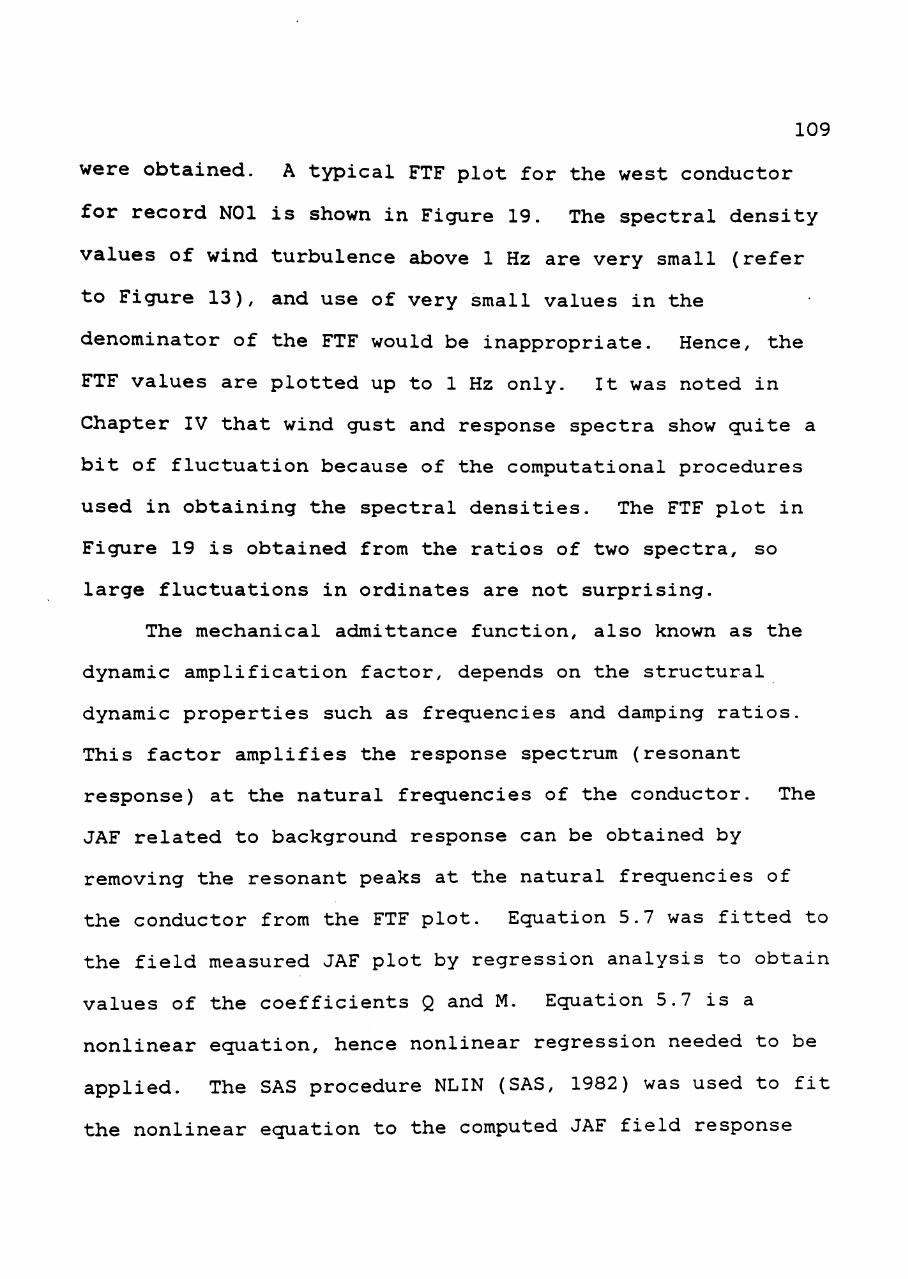
109
were obtained. A typical FTF plot for the west conductor
for record NOl is shown in Figure 19. The spectral density
values of wind turbulence above 1 Hz are very small (refer
to Figure 13), and use of very small values in the
denominator of the FTF would be inappropriate. Hence, the
FTF values are plotted up to 1 Hz only. It was noted in
Chapter IV that wind gust and response spectra show cjuite a
bit of fluctuation because of the computational procedures
used in obtaining the spectral densities. The FTF plot in
Figure 19 is obtained from the ratios of two spectra, so
large fluctuations in ordinates are not surprising.
The mechanical admittance function, also known as the
dynamic amplification factor, depends on the structural
dynamic properties such as frecjuencies and damping ratios.
This factor amplifies the response spectrum (resonant
response) at the natural frecjuencies of the conductor. The
JAF related to background response can be obtained by
removing the resonant peaks at the natural frecjuencies of
the conductor from the FTF plot. Equation 5.7 was fitted to
the field measured JAF plot by regression analysis to obtain
values of the coefficients Q and M. Equation 5.7 is a
nonlinear ecjuation, hence nonlinear regression needed to be
applied. The SAS procedure NLIN (SAS, 1982) was used to fit
the nonlinear equation to the computed JAF field response
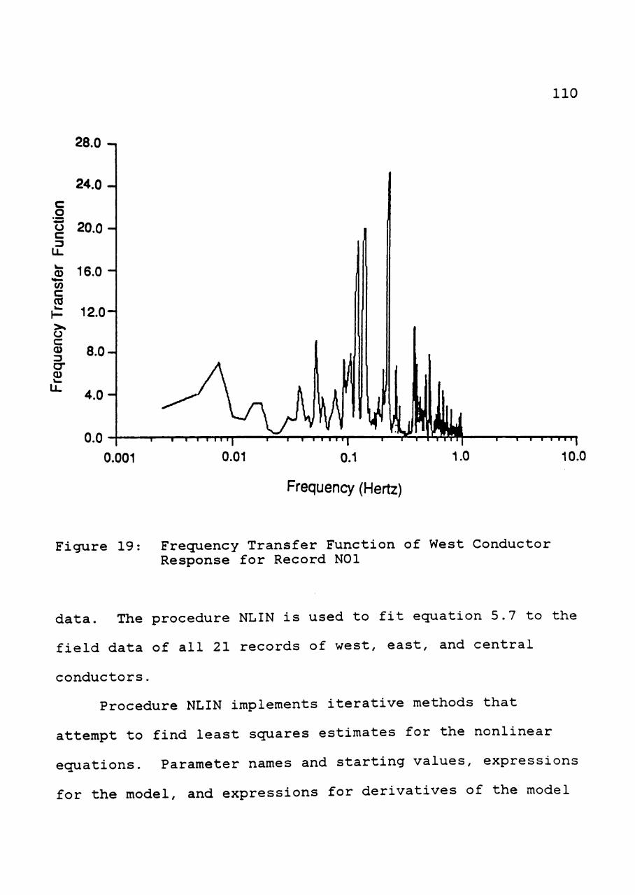
110
28.0 -,
I I I I 1 1 1 1 '
0.001 10.0
Frequency (Hertz)
Figure 19: Frecjuency Transfer Function of West Conductor Response for Record NOl
data. The procedure NLIN is used to fit ecjuation 5.7 to the
field data of all 21 records of west, east, and central
conductors.
Procedure NLIN implements iterative methods that
attempt to find least squares estimates for the nonlinear
equations. Parameter names and starting values, expressions
for the model, and expressions for derivatives of the model
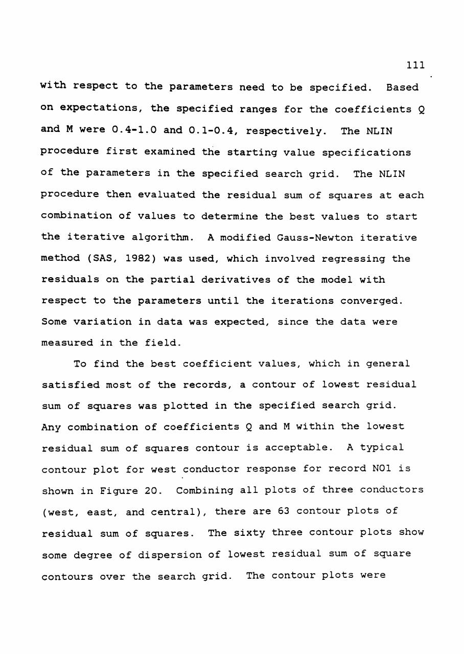
Ill
with respect to the parameters need to be specified. Based
on expectations, the specified ranges for the coefficients Q
and M were 0.4-1.0 and 0.1-0.4, respectively. The NLIN
procedure first examined the starting value specifications
of the parameters in the specified search grid. The NLIN
procedure then evaluated the residual sum of scjuares at each
combination of values to determine the best values to start
the iterative algorithm. A modified Gauss-Newton iterative
method (SAS, 1982) was used, which involved regressing the
residuals on the partial derivatives of the model with
respect to the parameters until the iterations converged.
Some variation in data was expected, since the data were
measured in the field.
To find the best coefficient values, which in general
satisfied most of the records, a contour of lowest residual
sum of scjuares was plotted in the specified search grid.
Any combination of coefficients Q and M within the lowest
residual sum of squares contour is acceptable. A typical
contour plot for west conductor response for record NOl is
shown in Figure 20. Combining all plots of three conductors
(west, east, and central), there are 63 contour plots of
residual sum of scjuares. The sixty three contour plots show
some degree of dispersion of lowest residual sum of scjuare
contours over the search grid. The contour plots were
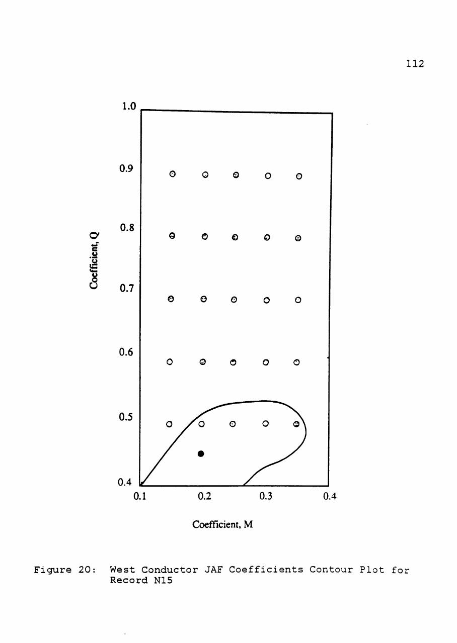
112
e (J
i
0.1 0.2 0.3 0.4
Coefficient, M
Figure 20: West Conductor JAF Coefficients Contour Plot for Record N15
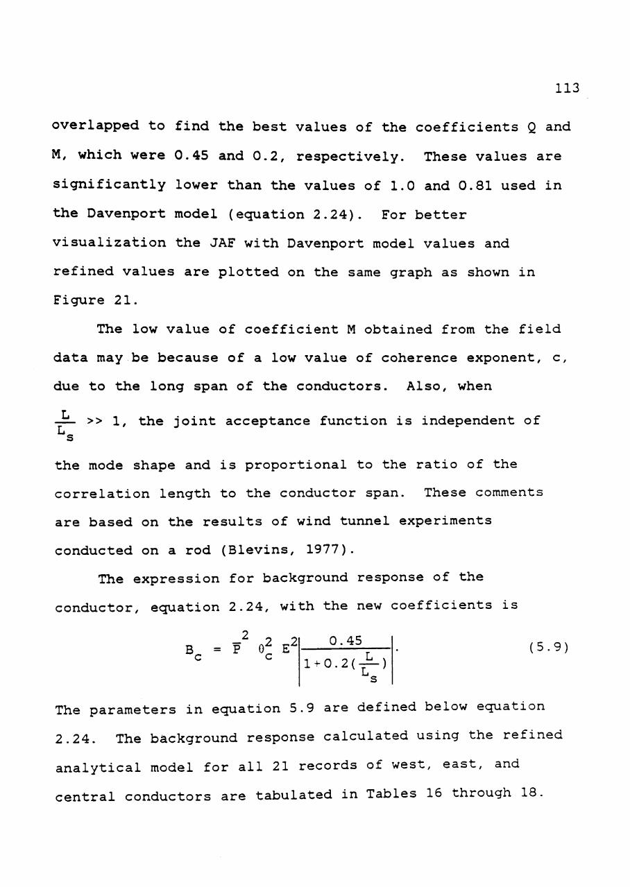
113
overlapped to find the best values of the coefficients Q and
M, which were 0.45 and 0.2, respectively. These values are
significantly lower than the values of 1.0 and 0.81 used in
tihe Davenport model (equation 2.24). For better
visualization the JAF with Davenport model values and
refined values are plotted on the same graph as shown in
Figure 21.
The low value of coefficient M obtained from the field
data may be because of a low value of coherence exponent, c,
due to the long span of the conductors. Also, when
-=- >> 1, the joint acceptance function is independent of ^s
the mode shape and is proportional to the ratio of the
correlation length to the conductor span. These comments
are based on the results of wind tunnel experiments
conducted on a rod (Blevins, 1977).
The expression for background response of the
conductor, ecjuation 2.24, with the new coefficients is
— ^ 2 2 B^ = P Ol E^
0.45
1 + 0.2(-^) ^s
(5.9)
The parameters in ecjuation 5.9 are defined below equation
2.24. The background response calculated using the refined
analytical model for all 21 records of west, east, and
central conductors are tabulated in Tables 16 through 18.
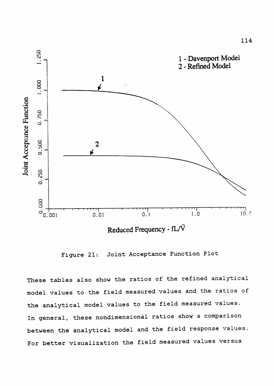
o CJ C
£ o c
o CJ
<
c 'o
o CM
O O o
o LT)
o o in
o
o o o -r 1 1 — I — I I M
0.001 0.0 ]
114
1 - Davenport Model 2 - Refined Model
- I 1 — I — r i l l -I 1 1—I—I I I "T 1 1—I—I I I I
0. 1.0 10.c
Reduced Frequency - fLA^
Figure 21: Joint Acceptance Function Plot
These tables also show the ratios of the refined analytical
model values to the field measured values and the ratios of
the analytical model values to the field measured values.
In general, these nondimensional ratios show a comparison
between the analytical model and the field response values.
For better visualization the field measured values versus
115
the refined analytical model values are plotted in Figure
22. The refined analytical model gave slightly better
predicted than the analytical model when Figures 22 and 17
are compared. In Tables 16 through 18, means and
coefficient of variations (COV) of the ensemble of the
ratios are shown. In each table, the mean of the ratio is
closer to 1 for the refined analytical model. However, the
COV for each conductor did not change. This improvement in
mean value of the ensemble and insignificant change in COV
value are due to inherent scatter in the field data.
Resonant Response
As noted earlier the analytical model overestimates the
resonant response. One of the reasons may be the use of low
damping ratio values as determined by ecjuation 2.26. Here
field measured resonant response data are used to estimate
damping ratios for the conductors.
Determining the Aerodynamic Damping
Ratio
As noted in Chapter II, three types of damping are
noted for conductor response, namely, material, structural,
and aerodynamic damping. For conductors aerodynamic damping
is very much higher than material or structural damping.
Therefore, both material and structural dampings are
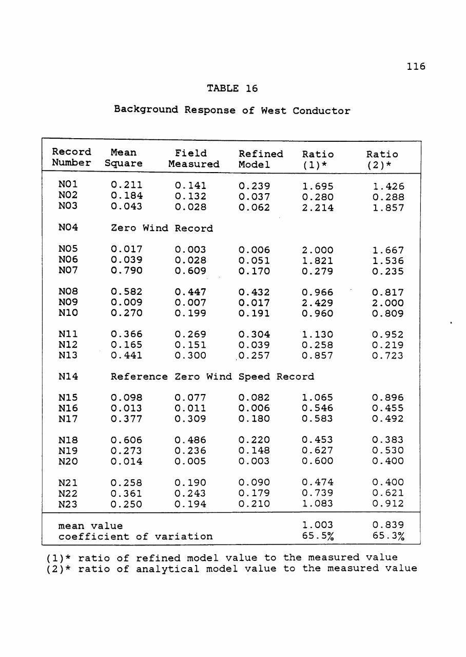
TABLE 16
Background Response of West Conductor
116
Record Number
rH
CM
CO
O
O
O
22
2
N04
N05 NO 6 NO 7
22
2 M
OO
O
vD
00
Nil N12 N13
N14
N15 N16 N17
22
2 to
M M
O
VD
00
rH
CM
C
O
CM
CM
C
M
2 2 2
Mean Scjuare
0.211 0.184 0.043
Field Measured
0.141 0.132 0.028
Zero Wind Record
0.017 0.039 0.790
0.582 0.009 0.270
0.366 0.165 0.441
0.003 0.028 0.609
0.447 0.007 0.199
0.269 0.151 0.300
Reference Zero Wind
0.098 0.013 0.377
0.606 0.273 0.014
0.258 0.361 0.250
mean value coefficient of
0.077 0.011 0.309
0.486 0.236 0.005
0.190 0.243 0.194
variation
Refined Model
0.239 0.037 0.062
0.006 0.051 0.170
0.432 0.017 0.191
0.304 0.039 ,0.257
Speed Rec
0.082 0.006 0.180
0.220 0.148 0.003
0.090 0.179 0.210
Ratio (1)*
1.695 0.280 2.214
2.000 1.821 0.279
0.966 2.429 0.960
1.130 0.258 0.857
ord
1.065 0.546 0.583
0.453 0.627 0.600
0.474 0.739 1.083
1.003 65.5%
Ratio (2)*
1.426 0.288 1.857
1.667 1.536 0.235
0.817 2.000 0.809
0.952 0.219 0.723
0.896 0.455 0.492
0.383 0.530 0.400
0.400 0.621 0.912
0.839 65.3%
(1)* ratio of refined model value to the measured value (2)* ratio of analytical model value to the measured value
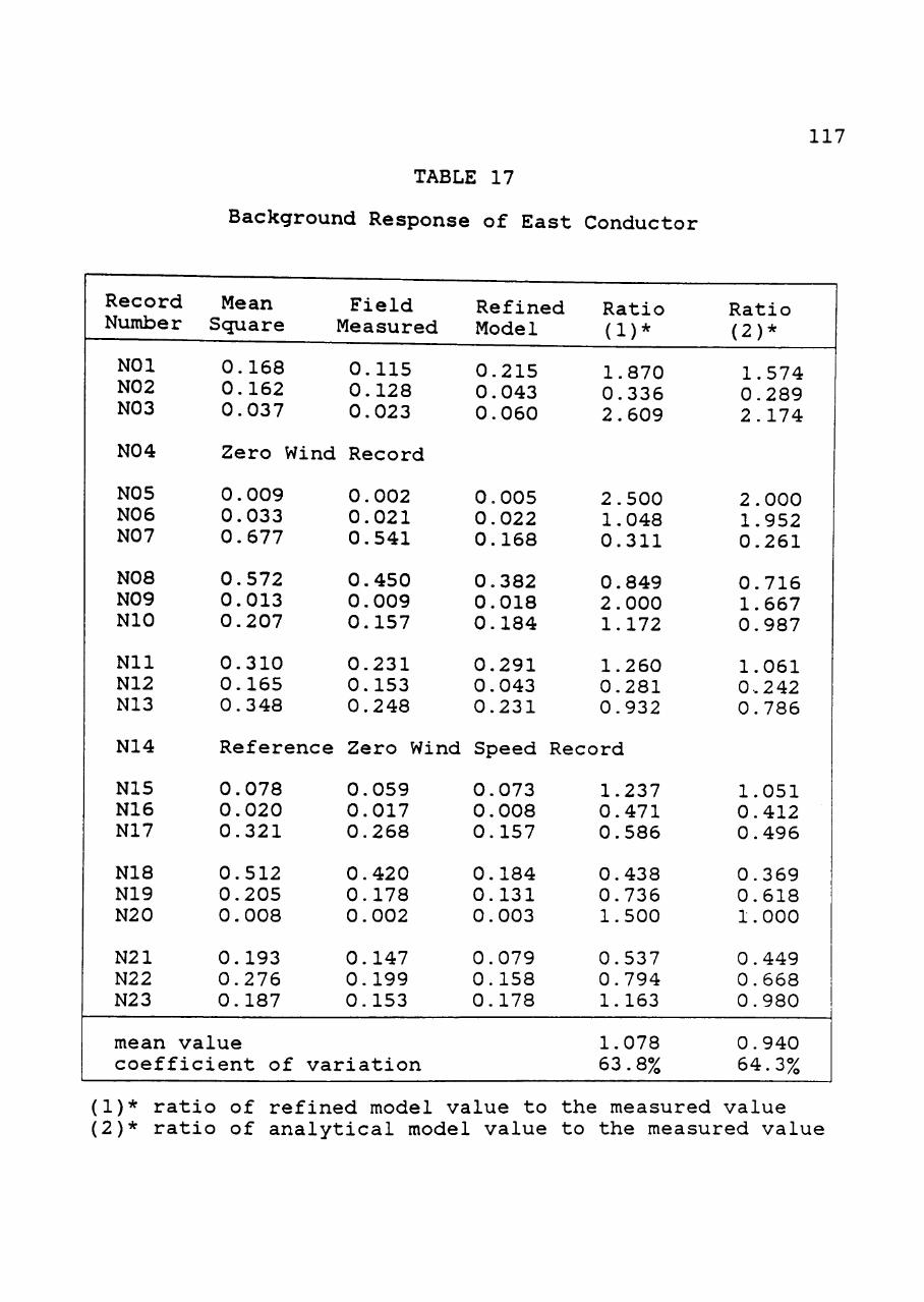
TABLE 17
Background Response of East Conductor
117
Record Number
NOl N02 N03
N04
Mean Scjuare
0.168 0.162 0.037
Field Measured
0.115 0.128 0.023
Zero Wind Record
Refined Model
0.215 0.043 0.060
Ratio (D*
1.870 0.336 2.609
Ratio (2)*
1.574 0.289 2.174
N05 NO 6 NO 7
N08 N09 NIC
Nil N12 N13
0.009 0.033 0.677
0.572 0.013 0.207
0.310 0.165 0.348
0.002 0.021 0.541
0.450 0.009 0.157
0.231 0.153 0.248
0.005 0.022 0.168
0.382 0.018 0.184
0.291 0.043 0.231
2.500 1.048 0.311
0.849 2.000 1.172
1.260 0.281 0.932
2.000 1.952 0.261
0.716 1.667 0.987
1.061 0.242 0.786
N14 Reference Zero Wind Speed Record
N15 N16 N17
N18 N19 N20
N21 N22 N23
mean
0.078 0.020 0.321
0.512 0.205 0.008
0.193 0.276 0.187
value coefficient of
0.059 0.017 0.268
0.420 0.178 0.002
0.147 0.199 0.153
variation
0.073 0.008 0.157
0.184 0.131 0.003
0.079 0.158 0.178
1.237 0.471 0.586
0.438 0.736 1.500
0.537 0.794 1.163
1.078 63.8%
1.051 0.412 0.496
0.369 0.618 1.000
0.449 0.668 0.980
0.940 64.3%
(1)* ratio of refined model value to the measured value (2)* ratio of analytical model value to the measured value
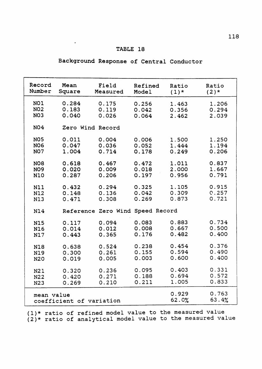
TABLE 18
Background Response of Central Conductor
118
Record Number
Mean Scjuare
Field Measured
Refined Model
Ratio (D*
NOl N02 N03
N04
NO 5 NO 6 NO 7
NOB N09 NIO
Nil N12 N13
N14
N15 N16 N17
N18 N19 N20
N21 N22 N23
0 .284 0 .183 0 .040
0 .175 0.119 0 .026
0 .256 0 .042 0 .064
1.463 0 .356 2 .462
Zero Wind Record
0.011 0.047 1.004
0.618 0.020 0.287
0.432 0.148 0.471
0.004 0.036 0.714
0.467 0.009 0.206
0.294 0.136 0.308
0.006 0.052 0.178
0.472 0.018 0.197
0.325 0.042 0.269
1.500 1.444 0.249
1.011 2.000 0.956
1.105 0.309 0.873
Reference Zero Wind Speed Record
0 .117 0 .014 0 .443
0 .638 0 .300 0 .019
0 .320 0 .420 0 .269
0 .094 0.012 0 .365
0 .524 0 .261 0.005
0 .236 0 .271 0.210
0 .083 0 .008 0 .176
0 .238 0 .155 0 .003
0 .095 0 .188 0 .211
0 .883 0 .667 0 .482
0 .454 0 .594 0 .600
0 .403 0 .694 1.005
mean value coefficient of variation
0.929 62.0%
Ratio (2)*
1.206 0 .294 2 .039
1.250 1.194 0 .206
0 .837 1.667 0 .791
0 .915 0 .257 0 .721
0 . 7 3 4 0 . 5 0 0 0 . 4 0 0
0.376 0 .490 0 .400
0 .331 0 .572 0 .833
0 .763 63.4%
(1)* ratio of refined model value to the measured value (2)* ratio of analytical model value to the measured value
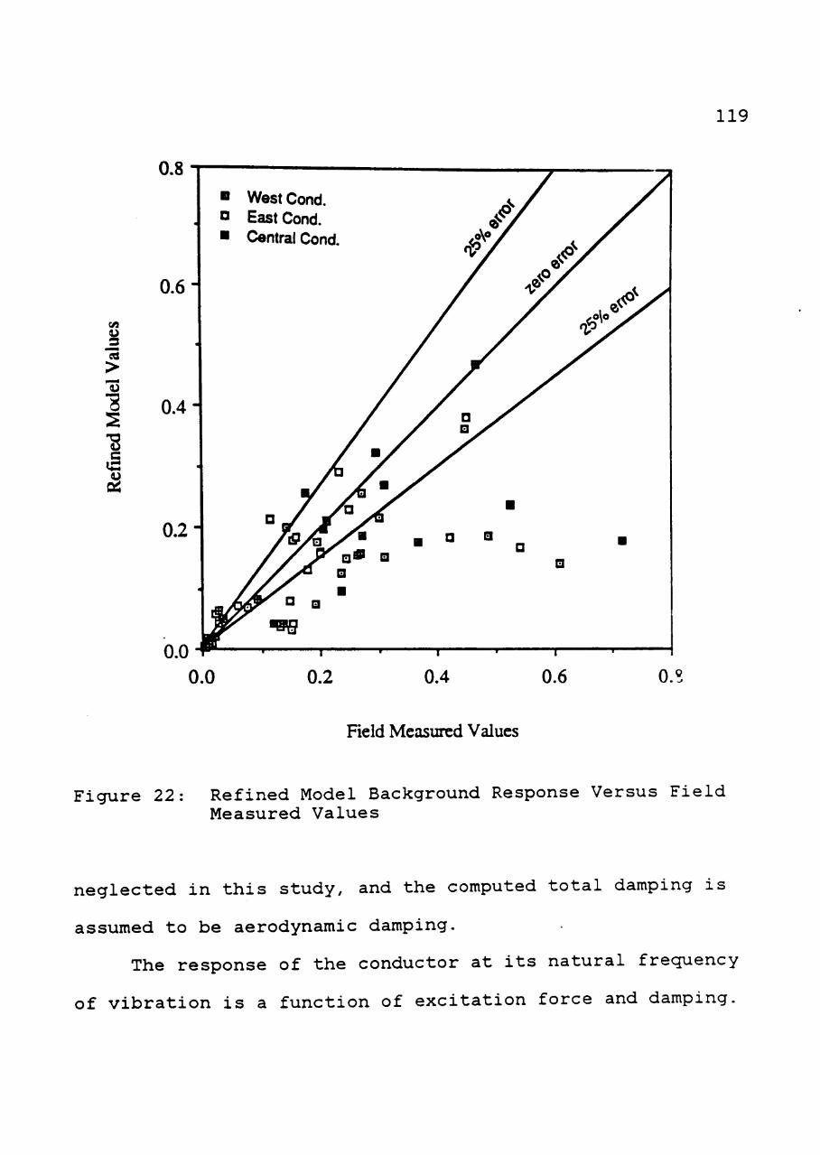
119
0.8
_3
>
•s c
0.6-
0.4-
" West Cond. D East Cond. • Central Cond
0.2-
0.0 0.2 0.4 0.6 0.
Field Measured Values
Figure 22: Refined Model Background Response Versus Field Measured Values
neglected in this study, and the computed total damping is
assumed to be aerodynamic damping.
The response of the conductor at its natural frequency
of vibration is a function of excitation force and damping.
120
The magnification factor method is used here to estimate the
aerodynamic damping ratio. For a single degree of freedom
system subjected to wind turbulence, the resonant peak is
amplified at a fundamental frecjuency of the conductor. The
height of this peak is controlled by the damping for the
conductor.
The frecjuency transfer function (Figure 19) described
in the previous section is used to establish damping. As
noted earlier, the FTF is a combination of aerodynamic
admittance function and the mechanical admittance function.
The mechanical admittance function amplifies the response at
the natural frecjuency of vibration of the conductor. The
expression for the mechanical admittance function is defined
in ecjuation 2.13. At the fundamental frecjuency of the
conductor, the ecjuation for the mechanical admittance
function simplifies as follows:
|H(f^)|^ = - V (-^ 4 C
where C = aerodynamic damping ratio, and
f = fundamental frecjuency of conductor.
The damping ratios of the conductors are determined
using the heights of the resonant peaks in the FTF plots.
As noted in Chapter III, the conductor spans on two sides of
Tower 16/4 are different. The natural frecjuencies of
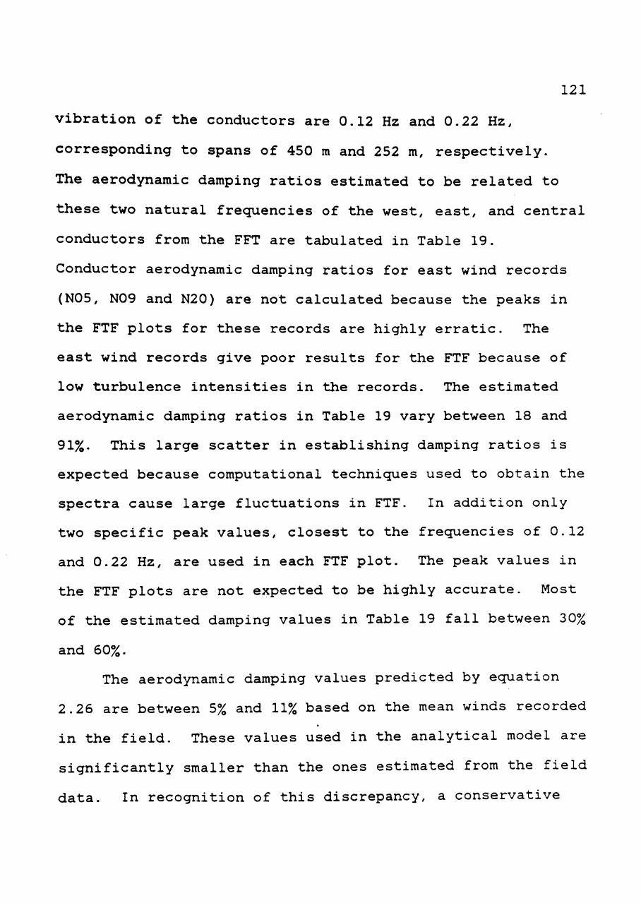
121
vibration of the conductors are 0.12 Hz and 0.22 Hz,
corresponding to spans of 450 m and 252 m, respectively.
The aerodynamic damping ratios estimated to be related to
these two natural frecjuencies of the west, east, and central
conductors from the FFT are tabulated in Table 19.
Conductor aerodynamic damping ratios for east wind records
(N05, N09 and N20) are not calculated because the peaks in
the FTF plots for these records are highly erratic. The
east wind records give poor results for the FTF because of
low turbulence intensities in tihe records. The estimated
aerodynamic damping ratios in Table 19 vary between 18 and
91%. This large scatter in establishing damping ratios is
expected because computational technicjues used to obtain the
spectra cause large fluctuations in FTF. In addition only
two specific peak values, closest to the frecjuencies of 0.12
and 0.22 Hz, are used in each FTF plot. The peak values in
the FTF plots are not expected to be highly accurate. Most
of the estimated damping values in Table 19 fall between 30%
and 60%.
The aerodynamic damping values predicted by ecjuation
2.26 are between 5% and 11% based on the mean winds recorded
in the field. These values used in the analytical model are
significantly smaller than the ones estimated from the field
data. In recognition of this discrepancy, a conservative
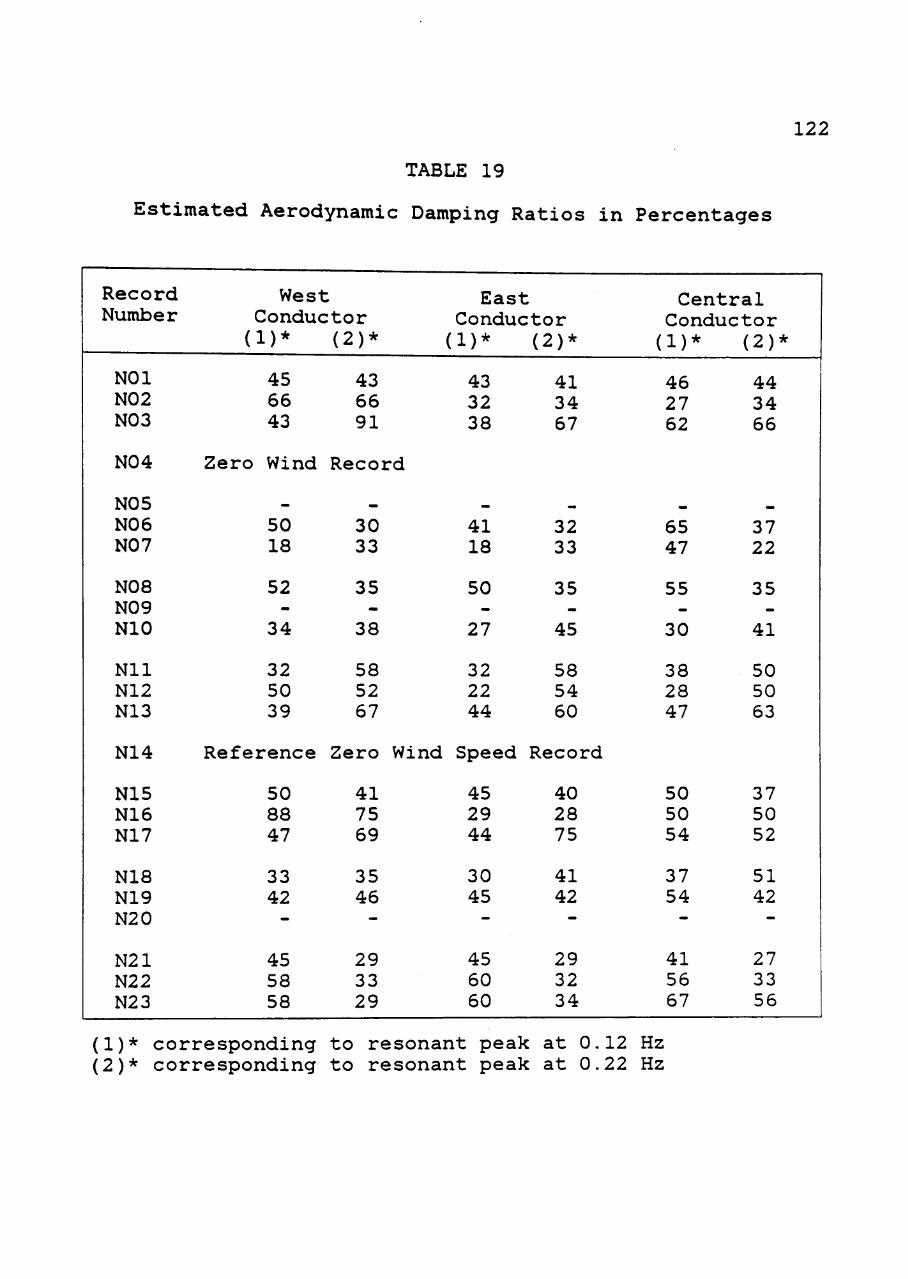
TABLE 19
122
Estimated Aerodynamic Damping Ratios in Percentages
Record Number
NOl N02 N03
N04
N05 NO 6 NO 7
NOB N09 NIO
Nil N12 N13
N14
N15 N16 N17
N18 N19 N20
N21 N22 N23
West Conductor (1)*
45 66 43
Zero Wind
_
50 18
52 -
34
32 50 39
Reference
50 88 47
33 42 -
45 58 58
(2)*
43 66 91
Record
_
30 33
35 -
38
58 52 67
Zero Wind
41 75 69
35 46 -
29 33 29
East Conductor (1)*
43 32 38
^
41 18
50 -
27
32 22 44
Speed
45 29 44
30 45 —
45 60 60
(2)*
41 34 67
^
32 33
35 -
45
58 54 60
Record
40 28 75
41 42 —
29 32 34
Central Conductor (1)*
46 27 62
^
65 47
55 —
30
38 28 47
50 50 54
37 54 —
41 56 67
(2)*
44 34 66
^
37 22
35 —
41
50 50 63
37 50 52
51 42 —
27 33 56
(1)* corresponding to (2)* corresponding to
resonant peak at 0.12 Hz resonant peak at 0.22 Hz
123
ensemble average value of 40% aerodynamic damping ratio is
suggested for conductors. Resonant responses are calculated
with this suggested aerodynamic damping for comparison
purposes.
Resonant Response with Suggested Damping Ratio
Resonant response values for all three (west, east, and
central) conductors are calculated using an aerodynamic
damping ratio of 40% in the analytical model. The values
are tabulated in Tables 20 through 22. The tables also show
the field measured resonant response and the total mean
scjuare value for each record.
In addition, ratios of resonant responses obtained from
the analytical model with 40% damping to field measured
values and from the analytical model with damping from
ecjuation 2.26 to field measured values are shown in the
tables. Use of 40% damping improves the prediction of
resonant response significantly. Mean values of the ratios
for 40% damping are close to unity. The COV of the ratios
in the tables are not effected significantly, though this is
misleading. The mean values of the ratios of responses from
the analytical model with damping from ecjuation 2.26 are a
little more than 4; hence associated COV values of 45%
reflect a large variation.
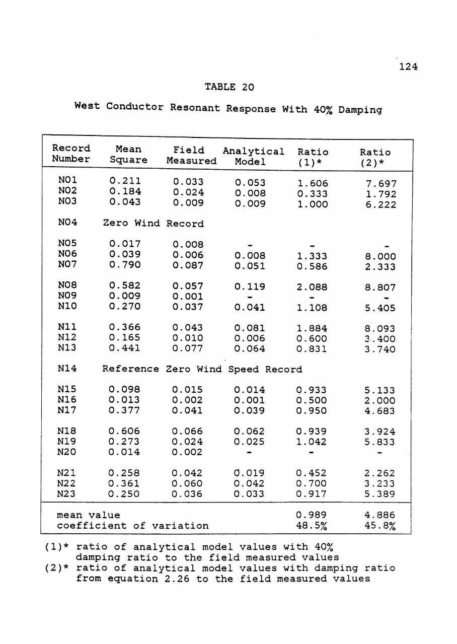
124
TABLE 20
West Conductor Resonant Response With 40% Damping
Record Number
NOl N02 N03
NO 4
NO 5 N06 NO 7
NOB N09 NIO
Nil N12 N13
N14
N15 N16 N17
N18 N19 N20
N21 N22 N23
Mean Scjuare
0.211 0.184 0.043
Zero Wind
0.017 0.039 0.790
0.582 0.009 0.270
0.366 0.165 0.441
Reference
0.098 0.013 0.377
0.606 0.273 0.014
0.258 0.361 0.250
mean value
Field Measured
0.033 0.024 0.009
Record
0.008 0.006 0.087
0.057 0.001 0.037
0.043 0.010 0.077
Zero Wind
0.015 0.002 0.041
0.066 0.024 0.002
0.042 0.060 0.036
coefficient of variation
Analytical Model
0.053 0.008 0.009
^
0.008 0.051
0.119 —
0.041
0.081 0.006 0.064
Speed Reco
0.014 0.001 0.039
0.062 0.025
-
0.019 0.042 0.033
Ratio (1)*
1.606 0.333 1.000
1.333 0.586
2.088 •
1.108
1.884 0.600 0.831
rd
0.933 0.500 0.950
0.939 1.042
-
0.452 0.700 0.917
0.989 48.5%
Ratio (2)*
7.697 1.792 6.222
8.000 2.333
8.807 .
5.405
8.093 3.400 3.740
5.133 2.000 4.683
3.924 5.833
-
2.262 3.233 5.389
4.886 45.8%
(1)* ratio of analytical model values with 40% damping ratio to the field measured values
(2)* ratio of analytical model values with damping ratio from ecjuation 2.26 to the field measured values
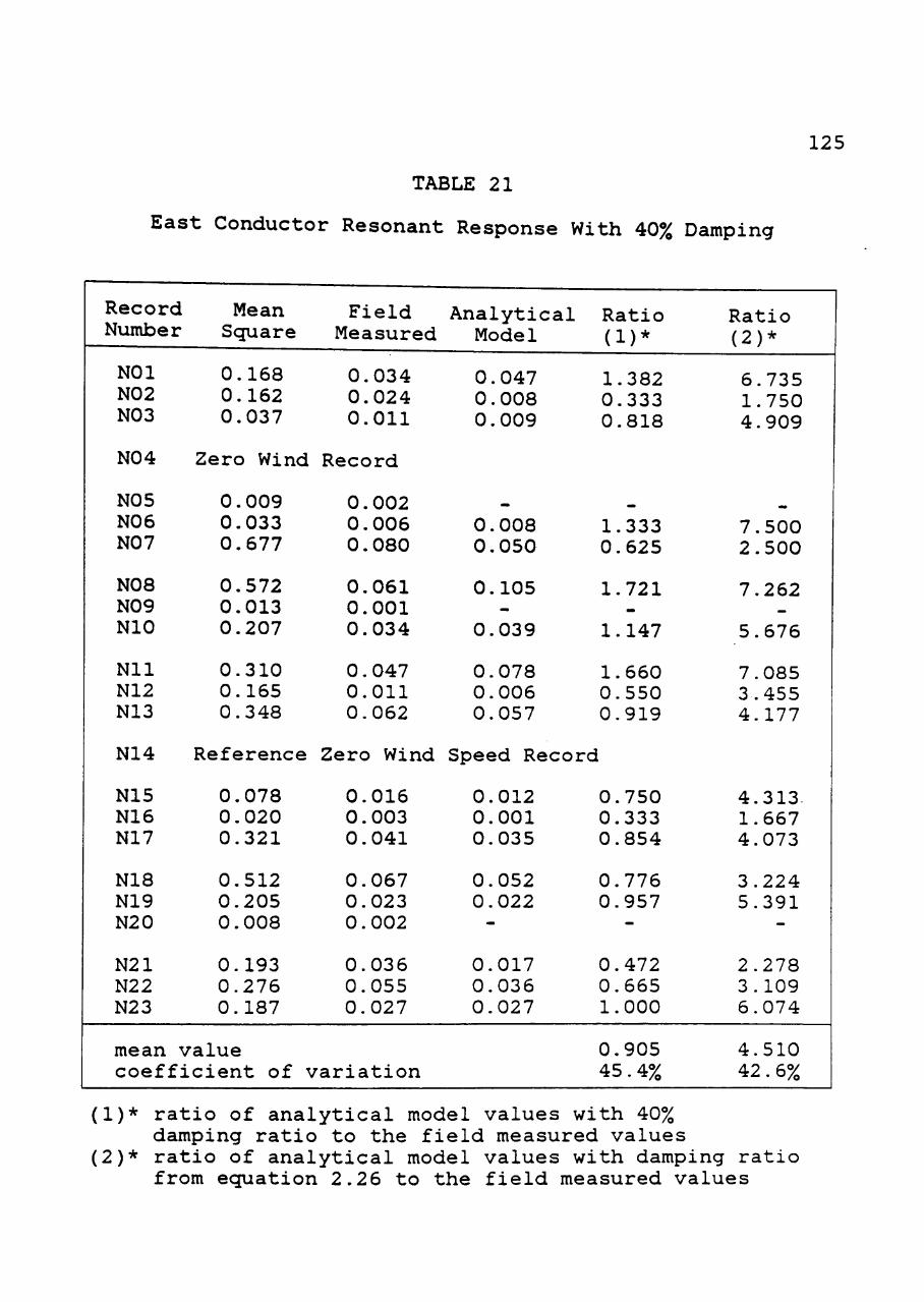
125
TABLE 21
East Conductor Resonant Response With 40% Damping
Record Number
NOl N02 N03
N04
N05 NO 6 N07
NOB N09 NIC
Nil N12 N13
N14
N15 N16 N17
N18 N19 N20
N21 N22 N23
Mean Scjuare
0.168 0.162 0.037
Zero Wind
0.009 0.033 0.677
0.572 0.013 0.207
0.310 0.165 0.348
Reference
0.078 0.020 0.321
0.512 0.205 0.008
0.193 0.276 0.187
mean value
Field Measured
0.034 0.024 0.011
Record
0.002 0.006 0.080
0.061 0.001 0.034
0.047 0.011 0.062
Zero Wind
0.016 0.003 0.041
0.067 0.023 0.002
0.036 0.055 0.027
coefficient of variation
Analytical Model
0.047 0.008 0.009
^
0.008 0.050
0.105 -
0.039
0.078 0.006 0.057
Ratio (1)*
1.382 0.333 0.818
.
1.333 0.625
1.721 •
1.147
1.660 0.550 0.919
Speed Record
0.012 0.001 0.035
0.052 0.022 -
0.017 0.036 0.027
0.750 0.333 0.854
0.776 0.957
-
0.472 0.665 1.000
0.905 45.4%
Ratio (2)*
6.735 1.750 4.909
7.500 2.500
7.262 _
5.676
7.085 3.455 4.177
4.313. 1.667 4.073
3.224 5.391
-
2.278 3.109 6.074
4.510 42.6%
(1)* ratio of analytical model values with 40% damping ratio to the field measured values
(2)* ratio of analytical model values with damping ratio from ecjuation 2.26 to the field measured values
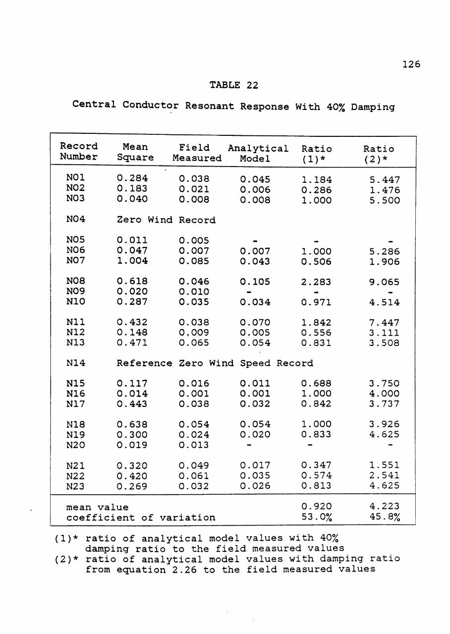
126
TABLE 22
Central Conductor Resonant Response With 40% Damping
Record Number
rH
CM
CO
O
O O
2
2 2
N04
N05 NO 6 NO 7
22
2 M
OO
O
vD
00
Nil N12 N13
N14
N15 N16 N17
2 2
2 to
M M
O
VD
00
rH
CM
CO
CM
C
M
CM
2 2 2
Mean Scjuare
0.284 0.183 0.040
Field Measured
0.038 0.021 0.008
Zero Wind Record
0.011 0.047 1.004
0.618 0.020 0.287
0.432 0.148 0.471
0.005 0.007 0.085
0.046 0.010 0.035
0.038 0,009 0.065
Analytical Model
0.045 0.006 0.008
0.007 0.043
0.105
0.034
0.070 0.005 0.054
Reference Zero Wind Speed Rec
0.117 0.014 0.443
0.638 0.300 0.019
0.320 0.420 0.269
0.016 0.001 0.038
0.054 0.024 0.013
0.049 0.061 0.032
mean value coefficient of variation
0.011 0.001 0.032
0.054 0.020
0.017 0.035 0.026
Ratio (D*
1.184 0.286 1.000
1.000 0.506
2.283
0.971
1.842 0.556 0.831
ord
0.688 1.000 0.842
1.000 0.833
0.347 0.574 0.813
0.920 53.0%
Ratio (2)*
5.447 1.476 5.500
5.286 1.906
9.065
4.514
7.447 3.111 3.508
3.750 4.000 3.737
3.926 4.625
1.551 2.541 4.625
4.223 45.8%
(1)* ratio of analytical model values with 40% damping ratio to the field measured values
(2)* ratio of analytical model values with damping ratio from equation 2.26 to the field measured values
127
For better visualization, a plot of the resonant
response predicted by the analytical model with 40% damping
versus the field measured resonant values is shown in Figure
23. This figure, when compared with Figure 18, shows that
the analytical model predicted better resonant values with
40% aerodynamic damping ratio. Figure 23 also illustrates
the inherent scatter in the field data.
Peak Factors
Another important component of the analytical model for
fluctuating response is the peak factor, g. It is used to
predict the peak response value that can occur in a time
segment. The peak factor is defined as the number of root
mean scjuare values by which the peak value exceeds the mean
value. The peak factor for field measured response data is
calculated using the ecjuation
g = JLJL_R (5.11) ^R
where ft = peak response value,
R = mean response value, and
<Tp = root mean scjuare of response.
The peak factor values vary depending on the averaging
time interval; the smaller the peak averaging time interval
the higher the peak factor value. The peak factors from the
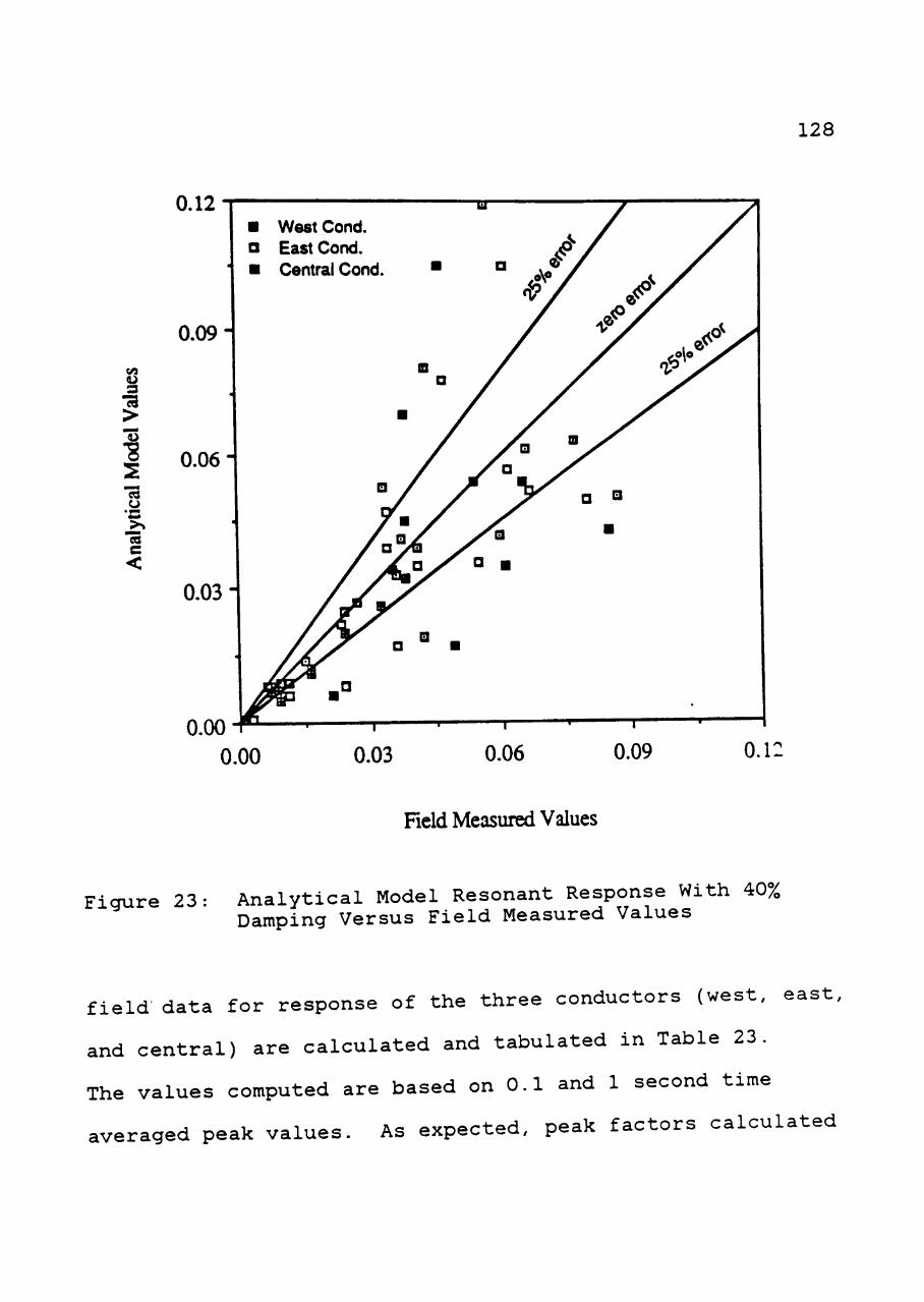
128
0.12
u 3 •a >
"8 :z "a u •c c
<
0.09-
• West Cond. a East Cond. • Central Cond
0.06-
0.03-
0.00 0.00 0.03 0.06 0.09 0.12
Field Measured Values
Figure 23: Analytical Model Resonant Response With 40% Damping Versus Field Measured Values
field data for response of the three conductors (west, east,
and central) are calculated and tabulated in Table 23.
The values computed are based on 0.1 and 1 second time
averaged peak values. As expected, peak factors calculated
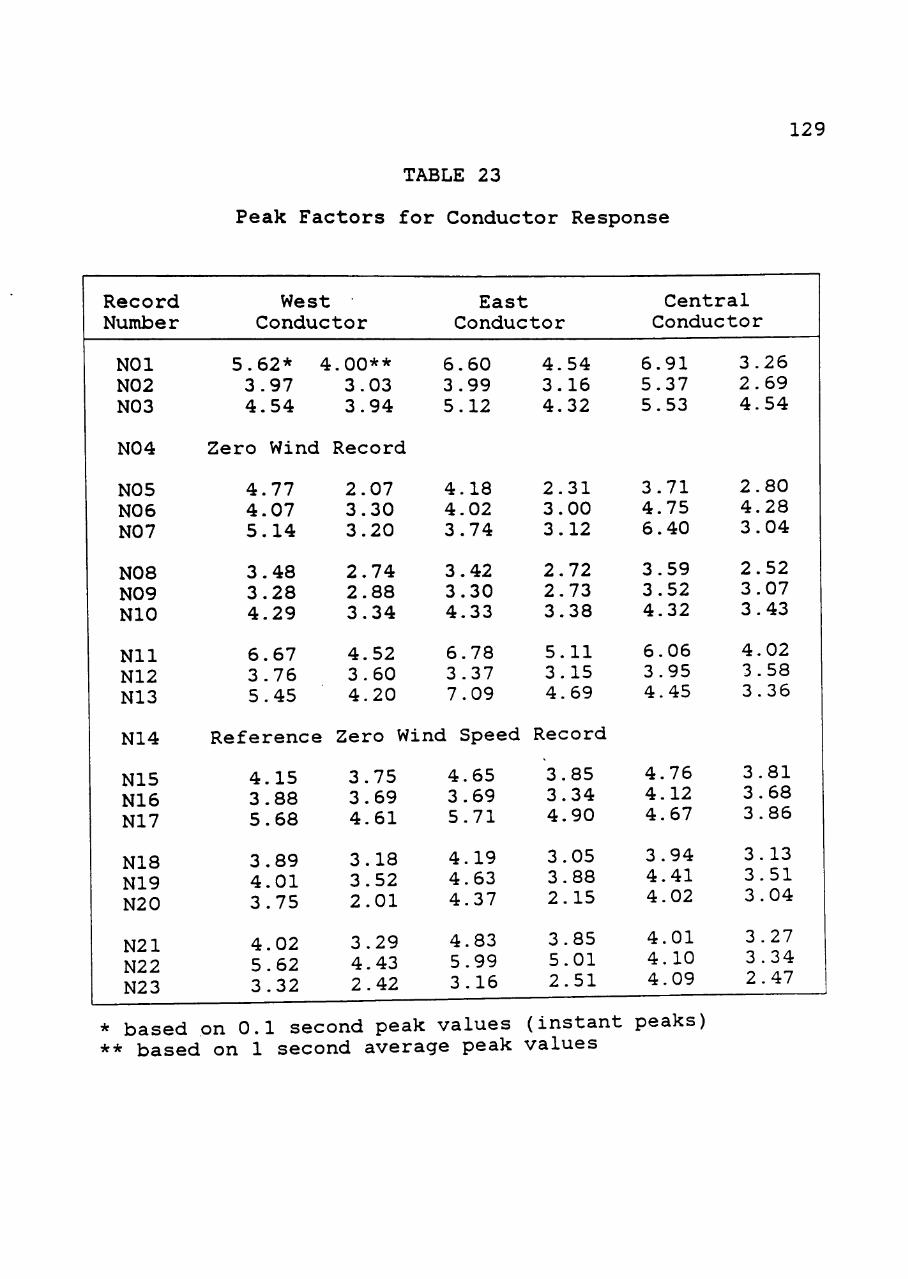
129
TABLE 23
Peak Factors for Conductor Response
Record Number
NOl N02 N03
NO 4
West Conductor
5.62* 4.00** 3.97 3.03 4.54 3.94
Zero Wind Record
East Conductor
6.60 4.54 3.99 3.16 5.12 4.32
Central Conductor
6.91 3.26 5.37 2.69 5.53 4.54
N05 NO 6 NO 7
NOB N09 NIC
Nil N12 N13
4.77 4.07 5.14
3.48 3.28 4.29
6.67 3.76 5.45
2.07 3.30 3.20
2.74 2.88 3.34
4.52 3.60 4.20
4.18 4.02 3.74
3.42 3.30 4.33
6.78 3.37 7.09
2.31 3.00 3.12
2.72 2.73 3.38
5.11 3.15 4.69
3.71 4.75 6.40
3.59 3.52 4.32
6.06 3.95 4.45
2.80 4.28 3.04
2.52 3.07 3.43
4.02 3.58 3.36
N14
N15 N16 N17
NIB N19 N20
N21 N22 N23
Reference Zero Wind Speed Record
* based on 0.1 second peak values (instant peaks) ** based on 1 second average peak values
4.15 3.88 5.68
3.89 4.01 3.75
4.02 5.62 3.32
3.75 3.69 4.61
3.18 3.52 2.01
3.29 4.43 2.42
4.65 3.69 5.71
4.19 4.63 4.37
4.83 5.99 3.16
3.85 3.34 4.90
3.05 3.88 2.15
3.85 5.01 2.51
4.76 4.12 4.67
3.94 4.41 4.02
4.01 4.10 4.09
3.81 3.68 3.86
3.13 3.51 3.04
3.27 3.34 2.47
130
for 0.1 second peaks are higher than those calculated for 1
second time average. The peak factors for 0.1 second time
averages range between 3.16 and 6.78, and for 1 second time
averages they range between 2.01 and 5.11. The suggested
range for peak factors in the analytical model is 3.5 to 4.0
(Davenport, 1980). Many records show that the peak factors
measured in the field are higher than 4.0. This is not
surprising in view of the fact that wind speed fluctuations
tend to be Gaussian, while the response fluctuations
associated with flow separation are often highly
intermittent, thus giving rise to large peak factors. The
peak factors vary from record to record and their
distribution functions are recjuired in order to establish
peak values with a specified probability of being exceeded.
Peak factors as function of the probability distribution of
upcrossings, or ecjuivalently, a specified number of
occurrences in a given interval of time, are obtained from
the field data.
Probabilistic Peak Factors from Field Data
For a stationary Gaussian process the cumulative
probability distribution in terms of upcrossings can be
stated as (refer to ecjuation 2.21).
131
2 P(>x) = exp - { - ^ 1 (5.12)
2 G^ X
where P(>x) = probability of upcrossing.
X - threshold level specified (=gCT ), and
CT - root mean scjuare.
The Rayleigh distribution function in ecjuation 5.12 can
be expressed in Weibull distribution form as
k P(>x) = exp -(-2.) (5.13)
where g = X /
and c , k = c o n s t a n t s .
Ecjuation 5 .13 can be expanded as
I n ( - I n P(>x) ) = k l n ( g ) - k l n ( c ) . ( 5 . 1 4 )
A graph of P(>x) versus x on an appropriate log scale
will yield k as the slope of the straight line and c as the
zero intercept.
Upcrossing rates were calculated for different
threshold values (multiples of RMS) of response of all three
conductors for each record. The field data used were the
0.1 second time interval responses. A linear regression
line was fitted for each record to assess trends with
132
respect to wind speed, wind direction, and turbulence
intensity. The conductor response data did not indicate any
specific trend for wind speed, wind direction or turbulence
intensity (terrain roughness). The upcrossing rates for
eighteen west wind records are plotted on the same graph, as
shown in Figure 24. Even though values have scatter, there
is a specific trend. A linear regression line is fitted to
the ensemble of data, as shown in Figure 24. The regression
line has a correlation coefficient of 0.93. This
correlation coefficient lends credence to the use of data as
an ensemble. Values for k and c in ecjuation 5.14 are 0.580
and 0.136, respectively.
For the Rayleigh distribution, values of k and c are 2
and 1.414, respectively. A line representing a Rayleigh
distribution is shown in Figure 24. The regression line
fitted to the field data is quite different from the
Rayleigh distribution line, indicating that the conductor
response data has a non-Gaussian distribution. It is
observed in Figure 24, that a Rayleigh distribution
underestimates upcrossing rate as compared to the field
data. The upcrossing rate plot can be used to determine the
peak factor for a desirable probability of upcrossings. The
peak factors obtained from the plot are based on 0.1 second
peak values.
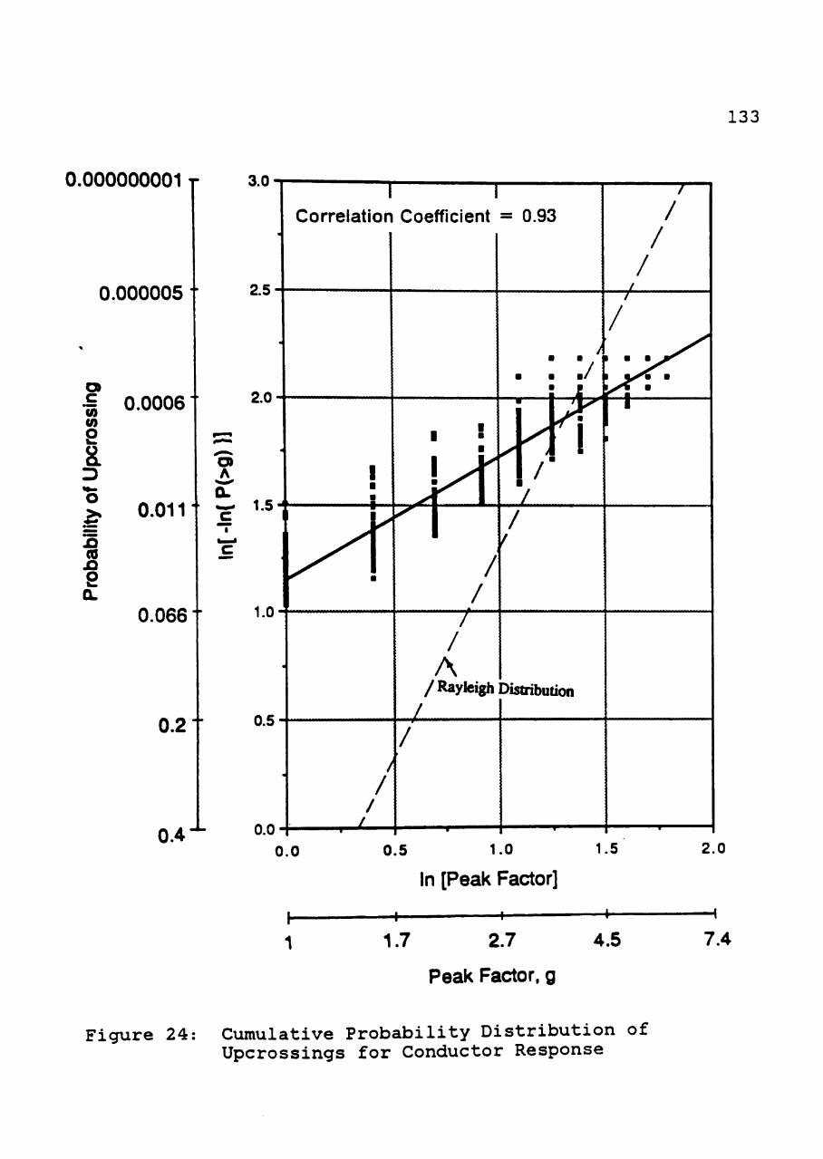
133
0.000000001 T
0.000005 •
o JO CO CO
9 D "o ! »
(0 n p
0.0006
0.0111 r
0.066"
A
0.2
0.4
1.7 2.7 4.5 7.4
Peak Factor, g
Figure 24: Cumulative P r o b a b i l i t y D i s t r i b u t i o n of Upcross ings for Conductor Response
CHAPTER VI
CONCLUSIONS
The purpose of this study was to compare and refine the
analytical model to predict dynamic responses of electrical
transmission line conductors to extreme winds using field
data. Wind and conductor response field data were obtained
from a full-scale field experiment. The field data were
collected by the Bonneville Power Administration (BPA) from
an instrumented single circuit 500 kV lattice tower on the
John Day-Grizzly line 2, which is located at the Moro site
in northern Oregon. The conductor spans 252 m and 450 m on
two sides of the instrumented tower. A total of
twenty-three twelve-minute duration records were utilized in
thi s study.
Based on the analysis of field data and the refinement
of the analytical model originally developed by Davenport
(1980), the following conclusions are made:
(1) The field measured wind and conductor response data
were found to be valid. The mean -responses of three
conductors were within 10% of each other for all
records. Fluctuating responses of the conductors
showed a significant amount of scatter.
134
135
(2) Winds traversing over the valley showed a wide
variation in profile and turbulence. Winds coming from
similar terrains of valleys and hills have a power-law
exponent range from 0.11 to 0.18 and a turbulence
intensity range from 0.11 to 0.21.
(3) The wind spectra showed 99% of spectral energy in the
frecjuency range below 1 Hz. The amplitude constant A
for Kaimal's gust spectrum was found to be within the
suggested range of 0.15 to 0.60; however, the exponent
constant n from the field data was much higher than the
suggested range of 0.33 to 0.67.
(4) The field measured effective conductor force
coefficient was found to vary between 0.48 and 0.75.
(5) Noticeable resonant peaks occurred in the frecjuency
range from 0.1 to 0.4 Hz. in the conductor response
spectra. Two of these peaks close to 0.12 and 0.22 Hz
were identified as corresponding to natural transverse
frecjuencies of the conductors associated with the two
unecjual spans. The resonant response energy level was
found to be low, less than 15% of the total energy in
most records.
(6) The majority of the records showed that the field
measured background turbulence response of the
conductors accounted for 75% of the fluctuating
response.
136
(7) The analytical model for background response was
refined by determining the joint acceptance function
(JAF) coefficients from the field measured data. The
best values for the coefficients (ecjuation 5.7) are
judged to be Q=0.45 and M=0.20.
(8) Damping of the conductors, found from the field
measured data, was much higher than the theoretical
aerodynamic damping ratio. A damping value of 40% is
suggested for the conductors.
(9) The refinement of JAF coefficients and use of
aerodynamic damping factor of 40% in the analytical
model gave a significant improvement in prediction of
background and resonant responses when results were
compared with the field measured data. However, ratios
of refined analytical model values to field measured
values showed a large scatter.
(10) Many records showed response peak factors (for 0.1
second response) to be higher than the range of 3.5-4.0
suggested in the analytical model. The upcrossing rate
principle was used to determine the peak factors on a
probabilistic basis. The Weibull distribution
satisfactorily describes the probability distribution
of the upcrossings rate.

137
It is recommended that additional field data be
obtained, particularly at reasonably predictable sites, to
further verify and refine the analytical model. The
computational procedures presented here are general and are
applicable to additional field data.
REFERENCES
ANSI, 1982: "Minimum Design Loads for Building and Other Structures, ANSI 58.1-1982," American National Standards Institute, Inc., ANSI, New York, NY.
ASCE, 1984: "Guidelines for Transmission Line Structural Loading," American Society of Civil Engineers, New York, NY.
Bendat, J.S., and Piersol, A.G., 1966: "Measurements and Analysis of Random Data," John Wiley and Sons, Inc., New York, NY.
Bendat, J.S., and Piersol, A.G., 1980: "Engineering Applications of Correlation and Spectral Analysis," John Wiley and Sons, Inc., New York, NY.
Blevins, R.D., 1977: "Flow-Induced Vibration," Von Nostrand Reinhold Company, New York, NY.
Brunt,. S.D., 1952: "Physical and Dynamical Meteorology," Second Edition, Cambridge University Press, England.
Chatfield, C , 1975: "The Analysis of Time Series: Theory and Practice," Chapman and Hall, London.
Criswell, M.E., and Vanderbilt, M.D., 1987: "Reliability-Based Design of Transmission Line Structures: Final Report," EPRI EL-4793, Project 1352-2, Vol. I, EPRI, Palo Alto, California, March.
Davenport, A.G., 1960: "Wind Loads on Structures," Technical paper No. 88 of the Division of Building Research, National Research Council of Canada, March.
Davenport, A.G., 1961: "The Application of Statistical Concepts to the Wind Loading of Structures," Proceedings of Institute of Civil Engineers, Vol. 19, pp. 449-471, August.
Davenport, A.G., 1967: "Gust Loading Factors," Journal of the Structural Division, Vol. 93, ST3, ASCE, New York, NY, pp. 11-34, June.
138
139
Davenport, A.G., 1972: "Approaches to the Design of Tall Buildings Against Wind," Theme Report, Proceedings of the ASCE-IABSE International Conference on Planning and Design of Tall Buildings, Lehigh University, pp. 1-22, August.
Davenport, A.G., 1977: "The Prediction of the Response of Structures to Gusty Wind," Proceedings of International Research Seminar, Safety of Structures Under Dynamic Loading, Vol. I, Norwegian Institute of Technology, Trondheim, Norway, pp. 257-284, June.
Davenport, A.G., 1980: "Gust Response Factors for Transmission Line Loading." Wind Engineering, Proc. of the Fifth International Conference on Wind Engineering, J.E. Cermak, Ed. (Fort Collins, CO; July 1979), Pergamon Press, New York, NY.
Ferraro, V., 1983: "Transverse Response of Transmission Lines to Turbulent Winds." Masters Thesis, The University of Western Ontario, London, Ontario, Canada, July.
GAI Consultants, Inc., 1981: "Transmission Line Wind Loading Research," EPRI Interim Report, RP 1277, EPRI, Palo Alto, California, April.
Ghiocel, D., and Lungu, D., 1975: "Wind Snow and Temperature Effects on Structures based on Probability," Abacus Press, Kent, England.
Gould, P.L., and Abu-Sitta, S.H., 1980: "Dynamic Response of Structures to Wind and Earthcjuake Loading, " John Wiley and Sons, Inc., New York, NY.
IMSL, 1982: International Mathematical and Statistical Libraries, Inc., Vol. 2.
Jan, Con-Lin, 1982: "Analysis of Data for the Response of Full-Scale Transmission Tower Systems Real Winds," Masters thesis, Texas Tech University, Lubbock, Texas, December.
Jenkins, G.M, and Watts, D.G., 1968: "Spectral Analysis and its Applications," Holden-Day, San Fransisco, California.
Kaimal, J.C, 1978: "Horizontal Velocity Spectra in an Unstable Surface Layer," Journal of the Atmospheric Sciences, Vol. 35, pp. 18-24.

140
Kancharla, V.S., 1987: "Analysis of Wind Characteristics from Field Wind Data," Masters thesis, Texas Tech University, Lubbock, Texas, May.
Kempner, L., Jr., 1979: "Wind Loading on a Latticed Transmission Tower," Report No. ETKA-79-1, Bonneville Power Administration, U.S. Dept. of Energy, November.
Kempner, L., Jr., and Laursen, H.I., 1977: "Response of a Latticed Transmission Tower," Report No. ETB-77-1, Bonneville Power Administration, U.S. Dept. of Energy, November.
Kempner, L., Jr., and Laursen, H.I., 1981: "Measured Dynamic Response of a Latticed Transmission Tower and Conductors to Wind Loading," Report No. ME-81-2, Bonneville Power Administration, U.S. Dept. of Energy, July.
Kempner, L., Jr., and Thorkildson, R.M., 1982: "Moro Test Site Wind Parameter Study." Report No. ME-82-3, Bonneville Power Administration, U.S. Dept. of Energy, December.
Kempner, L., Jr., Volpe, H.W., and Thorkildson, R.M., 1985: "Wind Loading Research on Transmission Line," Proceedings of the Fifth International Conference on Wind Engineering, Texas Tech University, Lubbock, Texas, November.
Kim, Soo-Il, 1977: "Wind Loads on Flat Roof Area Through Full-Scale Experiment," Doctoral Dissertation, Texas Tech University, Lubbock, Texas.
Lawson, T.V., 1980: "Wind Effects on Buildings: Vol. 1, Design Applications," Applied Science Publishers, Ltd., London, England.
Levitan, M., 1987: Unpublished Data, Civil Engineering Department, Texas Tech University, Lubbock, Texas.
Mehta, K.C., Norville, H.S., and Kempner, L., Jr., 1986: "Electric Transmission Structure Response to Wind," Proc. International Symposium on Probabilistic Methods Applied to Electric Power Systems, Samy Krishnasamy, Ed., (Ontario Hydro, Toronto, Canada; July 1986), Pergamon Press, New York, NY.

141
Melbourne, W.H., 1975: "Peak Factors for Structures Oscillating Under Wind Action." Proc, Fourth International Conference on Wind Effects on Buildings and Structures, Cambridge University Press, London, England.
Miller, I., and Freund, J.E., 1977: "Probability and Statistics for Engineers," Second ed., Prentice-Hall, Inc., Englewood Cliffs, New Jersey.
NESC, 1984: "National Electric Safety Code," ANSI C2, Institute of Electrical and Electronics Engineers, Inc., Wiley-Interscience, New York, NY.
Nigam, N.C., 1983: "Introduction to Random Vibrations," The MIT Press, Cambridge, Massachusetts, London, England.
Norville, H. S., K.C. Mehta, andA.F. Farwagi, 1985: "500 kV Transmission Tower/Conductor Wind Response: phase I," Institute for Disaster Research, Texas Tech University, Lubbock, Texas, May.
NRCC, 1980: "National Building Code of Canada," NRCC No. 17724, Associate Committee on the National Building Code, National Research Council of Canada, Ottawa, Canada.
Potter, J.L., and Boylan, D.E. 1981: "Aerodynamic Force Coefficients for the Prediction of Wind Loads on Electrical Transmission Lines," Sverdrup Corporation, Report submitted to EPRI, Palo Alto, California.
Pries, R.A., 1981: "Moro 1200 kV Structural/Mechanical Test Program," Report No. ME-81-1, Bonneville Power Administration, U.S. Dept. of Energy, March.
Racicot, R.L., 1969: "Random Vibration Analysis-Application to Wind Loaded Structures," Report No. 30, School of Engineering, Case Western Reserve University, Cleveland, Ohio, February.
Rice, S.O., 1945: "Mathematical Analysis of Random Noise," Bell System Technical Journal, Vol. 24, pp. 46-156.
Sachs, P., 1978: "Wind Forces in Engineering," Second Edition, Pergamon Press, New York.
Simiu, E., and Scanlan, R.H., 1985: "Wind Effects on Structures: An Introduction to Wind Engineering," John Wiley and Sons, Inc., New York, NY.
142
Statistical Analysis System (SAS), 1985: "SAS User Guide: Statistics," SAS Institute, Inc., Gary, North Carolina.
Symon, R.K., 1961: "Mechanics," Second Ed., Addison-Wesley Publishing Co., Inc., Reading, MA, May.
Twu, S.R., 1983: "Gust Response Factor for Transmission Line Structures," Masters Thesis, Texas Tech University, Lubbock, Texas, August.