resource abundance and economic growth in...

Resource Abundance and Economic Growth in China∗

Rui Fan † Ying Fang ‡ Sung Y. Park §

[ Forthcoming at China Economic Review ]

Abstract

This paper revisits the resource curse phenomenon in China and differs from the previous stud-ies in four respects: (i) City-level data is used; (ii) A spatial variable is constructed to estimatethe diffusion effect of natural resources among cities in the same province; (iii) The impact of re-source abundance on economic development is investigated not only at the city level but also at theprefectural level in China; (iv) We use a functional coefficient regression model to deal with city-specific heterogeneity and, at the same time, analyze the transmission mechanism of the resourcecurse phenomenon. Our empirical results show that there is no significant evidence to support theexistence of a resource curse phenomenon in China. On the other hand, we find that the degreeof natural resource abundance in a city has a positive diffusion effect on the economic growth ofneighboring cities within the same province at the city level, but not at prefectural levels. Weattribute this to the urban bias policy.

Key words: Resource curse; Diffusion effects; Transmission channels; Functional coefficientmodel. JEL code: O13; O18

∗The previous title of this paper was “Diffusion Effects or Curse of Resources? An Evidence from China”. Theauthors would like to thank Zhigang Li, Yiu Por Che, Chun-Chung Au and the participants in conferences and semi-nars in Young Economist Society (YES), Xiamen University, April 3-4, 2010, Brownbag Seminar at WISE, XiamenUniversity, May 15, 2010, and Chinese Economists Society (CES), Xiamen University, June 19-21, 2010 for manypertinent comments and discussions. We are grateful to the co-editor Xiaobo Zhang and two anonymous referees fortheir valuable comments. However, we retain the responsibility for any remaining errors. We thank Li Chen for hisexcellent research assistance. Fang’s research is partially supported by the National Natural Science Foundation ofChina 70971113 and by the Fundamental Research Funds for the Central Universities 2010221092.

†Department of Economics, University of Illinois at Urbana-Champaign, Champaign, IL 61820, U.S.A.‡The Wang Yanan Institute for Studies in Economics, MOE Key Laboratory of Econometrics, and Fujian Key

Laboratory of Statistical Sciences, Xiamen University, Xiamen, Fujian 361005, China.§Corresponding Author: Department of Economics, The Chinese University of Hong Kong, Shatin, NT, Hong

Kong, China. Tel: +852-2609-8001, Fax: +852-2603-5805. Email: [email protected].

1

1 Introduction

Many studies attempt to determine whether or not natural resources serve as an important en-

gine for economic growth. Their common finding is that the economic growth rates of natural

resource-abundant countries are slower than those of natural resource-scarce economies (Leite and

Weidmann, 1999; Papyrakis and Gerlagh, 2004; Rodriguez and Sachs, 1999; Sachs and Warner,

1995, 1997, 1999, among many others). This widely accepted phenomenon is referred to as the

“resource curse” in the literature. Moreover, some recent studies analyze which socio-economic

variables yield a negative association between economic growth and natural resource abundance.

For example, Gelb (1988) and Auty (1990) argue that resource rich countries are likely to pay

more attention to rent-seeking behavior rather than other productive activities. Angrist and Kugler

(2008) emphasize that abundant resources can be a source of civil conflict. Matsuyama (1992)

and Sachs and Warner (2001) find that resource-abundant economies value their natural resource

oriented goods higher than their manufactured goods, which could keep their economies at a low

level of economic growth. Gylfason (2000) finds that the level of education is an important factor

for determining the resource curse phenomenon. Kronenberg (2004) demonstrates that corruption

is a major determinant for the appearance of the curse of natural resources. Papyrakis and Gerlagh

(2007) extend this line of research from cross-country studies to one examining different regions

within the same country. They investigate forty-nine U.S. states and find positive evidences of the

existence of the resource curse. In particular, they find that resource abundance decreases invest-

ment, schooling, openness and R&D expenditure and while increasing corruption.

However, a consensus among economists is far from reached about understanding the role nat-

ural resources play in economic growth. Habakkuk (1962) believes that resource abundance is one

of the main reasons the U.S. economy surpassed the U.K. economy in the 19th century. Wright

(1990) finds that the most significant feature of U.S. manufacturing exports during the early 20th

2

century was an intensity in natural resources, and that abundant resources reflect advanced tech-

nology. Davis (1995) analyzes twenty-two mineral-based economies using different criteria and

finds that the existence of resource curse is the exception rather than the rule. On the other hand,

many economists find that the negative association between resource abundance and economic

growth is not robust or insignificant when different measures of resource abundance and different

frequencies of data are used. Sala-i-Martin (1997) finds a negative association when the ratio of

primary products to exports is used, a measurement of resource abundance advanced by Sachs and

Warner (1995), while a positive association is obtained when the ratio of GDP to mining products

is employed. Stijns (2005) shows that resource curse disappears when the resource abundance is

measured in terms of energy and mineral reserves. Alexeev and Conrad (2009) argue that the cur-

rent finding of the existence of resource curse, obtained by using an average growth rate starting

from 1965, is possibly due to a dynamic pattern of refinement.

In recent years, more and more economists have become interested in examining whether the

resource curse exists in China. To the best of our knowledge, Zhang, Xing, Fan and Luo (2008)

is the first paper in the English literature to explore this important issue. Using provincial-level

data from 1985 to 2005, they find that Chinese provinces with abundant resources perform worse

than provinces with poor natural resources in terms of per capita consumption growth. However,

when they use the subperiod sample of 1995 to 2005, this finding disappears. They attribute this

change to the resource price liberalization launched in the mid-1990s. Xu and Wang (2006) em-

ploy provincial-level panel data from 1995 to 2003 and find evidence to support the existence of

resource curse. Using panel data of eleven western provinces between 1991 to 2006, Shao and Qi

(2009) verify the existence of resource curse in the western regions of China. Using the panel data

of twenty-eight provinces, Ji, Magnus and Wang (2010) find that although resource abundance has

a positive impact on economic growth in China, resource dependence has a negative impact. Fur-

thermore, using a varying-coefficient model, they find the effect of natural resource on economic

3

growth varies with institutional qualities. Fang, Ji and Zhao (2011) investigate the resource curse

in China using city-level data. They argue that the controversial results of the existence of the

resource curse partially result from using different resource abundance measures.

In this paper, we revisit the curse of resources in China and analyze possible transmission

mechanisms between resource abundance and economic development. Our paper contributes to

the literature in four respects:

(i) Instead of using province-level data, our analysis is based on all city-level data in China.1

Benefitting from the large number of prefectural-level observations, we adopt a cross-sectional

econometric model rather than a panel data model.2

(ii) A diffusion variable based on the relative degree of resource abundance and the geographic dis-

tances between cities is constructed to capture the spill-over effect of resource abundance among

cities within the same province. Hence, our study can distinguish two different effects. The ef-

fect of resource abundance represents whether the resource abundance of a city affects this city’s

long-run economic development, and the effect of the diffusion variable implies whether a city can

gain a benefit from resource-rich cities within the same province. To our knowledge, this is a new

contribution to the literature.

(iii) We investigate the impact of resource abundance on economic development not only at the

city level but also in the rural regions. We obtain different empirical outcomes for these cases.

This difference may result from the urban bias policy.

(iv) We analyze transmission mechanisms between resource abundance and economic develop-

ment by employing a functional coefficient regression model. To analyze the transmission mech-

1Fang, Ji and Zhao (2011) employ a sample consisting of only 95 cities in China.2Due the limited number of provincial-level observations in China, most studies employ a panel data model to

examine the existence of the resource curse. However, most cross-country studies prefer a cross-sectional regressionmodel rather than a panel data model. A panel data model usually assumes a fixed effect and a first-order differencemethod is adopted to estimate the within-group effect. After the first difference, one actually estimates the short-run ef-fect: using the change in resource abundance over periods to explain the economic growth rates of different provinces,while resource curse theory concentrates on the long-run effect of resource abundance on economic development.

4

anisms, many studies adopt two least squares regressions separately (see Papyrakis and Gerlagh,

2004, 2007; Shao and Qi, 2009; Fang, Ji and Zhao, 2011; among others). Due to these two sepa-

rated regressions, it is different to infer whether a particular transmission mechanism is important

to the relationship between resource abundance and economic growth. Taking advantage of the

functional coefficient regression, we can combine the two regressions into one and make a precise

inference about the transmission mechanism. Moreover, this functional coefficient regression al-

lows us to capture a nonlinear relationship between resource richness and economic development,

providing some interesting economic stories that may be neglected in a simple linear model.

Our results show that there is no support for the existence of resource curse phenomenon at

the city level in China over the period 1997-2005. By applying the functional coefficient regres-

sion model, we find that the estimated effects of natural abundance on the economic growth of

regional economies are significantly positive when the relative scale of the manufacturing indus-

try, innovation (R&D) and openness are considered as transmission channels. In particular, we find

a nonlinear relationship between natural resources and economic growth, which indicates that one

unit of natural resources affects the growth of the regional economy differently depending on the

levels of the transmission variables. We believe that this result is useful for Chinese policy makers

to establish appropriate economic and political policies. Moreover, our empirical results for the

diffusion effect show that an abundance of natural resources not only encourages local economic

development but also boosts growth of the economy in other cities in the same province. This

diffusion phenomenon is significant through the economic transmission channels such as manu-

facturing, innovation, human capital investment and openness at the city level but is not significant

at the prefectural level. We attribute this difference to the urban bias policy.

The next section discusses different measurements for resource abundance in China and their

possible impacts on empirical results. Section 3 introduces the basic model and the construction

of the diffusion variable. We also investigate the impact of resource abundance on economic de-

5

velopment at the city level and in rural regions as well. Section 4 analyzes possible transmission

mechanisms using the functional coefficient regression model, and the last section concludes.

2 Resource Abundance Measures

Most of the studies examining the resource curse in China measure resource abundance as shares

of GDP or as another economic variable highly related to economic growth, such as total industrial

output and total fixed investment. For example, Zhang, et al.,(2008) measure resource intensity

as the ratio of resource production to total GDP; Xu and Wang (2006) consider a share of fixed

investment in the mining industry compared to total fixed investment as an indicator of resource

abundance; and Shao and Qi (2009) adopt the ratio of outputs in the energy industry to total in-

dustrial output as a measure of resource abundance. We find that the results favoring the existence

of the resource curse in previous literature may be misleading because while the economic growth

rate is adopted as a dependent variable in the regression model, at the same time, resource abun-

dance in the regression model is expressed as a share of an economic variable which itself reflects

economic growth.

Fang, et al.,(2011) compute the average value of the energy output of Shandong, Jiangshu,

Shanxi, Ningxia, Gansu and Qinghai provinces between 1989 and 2006. Among these six provinces,

Shandong has the largest value of energy output followed in descending order by Shanxi, Jiangshu,

Ganshu, Ningxia and Qinghai. However, when resource abundance is measured by the ratio of the

energy output to total industrial output, Ningxia becomes the most resource-rich province while

Jiangshu and Shandong are recognized as the least and the second least resource-rich provinces,

respectively. If resource abundance is measured by a share of GDP or of other variables highly

related to economic growth, then a region with low economic growth performance tends to be

recognized as a resource-abundant region, such as Ningxia province in the above example, which

6

leads to results in favor of finding the resource curse in China (Alexeev and Conrad, 2009).

In this paper, we follow Fang, et al.,(2011) and measure resource abundance by the average

fraction of workers in the mining industry compared to the total population in the same city be-

tween 1997 and 2005. The mining industry is directly related to most natural resources including

coal, oil, natural gas, metal and nonmental ores and other resources. The merit of our measure-

ment lies in the delinking of resource abundance to economic growth. However, our measurement

of resource abundance may not be ideal also. For example, the mining industry is not the only

industry related to natural resources. Soil and water resources are also very important influences

of economic growth in China. Heerink, Bao, Li, Lu and Feng (2009) and Qu, Kuyvenhoven, Shi

and Heerink (2010) discuss the usage of soil and water resources in the rural areas of China. Al-

ternatively, it may be better to adopt some direct measure of resource production or of resource

reserves. However, resource production and reserves data are not available at the city level.

3 Testing the Resource Curse Using Prefectural City-level Data

3.1 The Basic Model and the Diffusion Effect

Many empirical studies analyzing the resource curse consider a linear empirical growth regression

model. We start with the following basic model:

Gi = α0 + α1 ln Y1990,i + α2miningi + z′iξ + ui, (1)

where Gi denotes the growth rate of GDP per capita of a city i from 1997 to 2005, that is, Gi =

ln(Y2005,i/Y1997,i), Y1990,i is the initial GDP per capita of a city i in 1990, miningi is the logarithm of

the average fraction of workers who are in the mining industry in a city i from 1997 to 2005, zi and

ξ are the vectors of the other demographic variables and their corresponding parameter vectors,

respectively, and ui denotes the disturbance term. Coefficient α2 reflects the impact of resource

7

abundance in a city on its own economic development. A significant and negative sign for α2

indicates the existence of the resource curse.

Since the local government of a province has independent authority for the distribution of

economic resources, including natural resources, the interacting behavior among cities in the same

province could provide useful information for making policy decisions. Thus, it is of interest to

investigate how a city can benefit from the resource abundance of its neighborhood within the

same province. In other words, we want to know whether the hypothesis that “because resource-

rich cities in my province are my neighbors, my city is better off” is true. We denote this spill over

effect among cities a so-called diffusion effect.

In order to define the variable that measures the diffusion of natural resources, we need to

consider two things. First, we need to define the direction of the diffusion. The diffusion effect

between two cities can be categorized as either uni-directional or bi-directional. For simplicity, we

assume that only a resource-rich city may influence a resource-poor city. However, when two cities

in the same neighborhood have a similar amount of natural resources, the diffusion process can be

bi-directional. Second, we need to define the neighborhood carefully. We denote cmk as an m-th city

located in k-th province, where m = 1, 2, · · · ,Mk and k = 1, 2, · · · ,K. Since provinces are endowed

to relatively independent distribution rights of natural resources, we set the maximum boundary

of the neighborhood of m-th city in k-th province as the physical boundary of k-th province, say,

Pk. For each city m in province k, cmk, we can construct a ball, Bmk ∈ Pk, which represents the

neighborhood of cmk. Then for each province k, we can define a variable that represents the spill

over phenomenon from c jk to cmk for j , m,or

UUm ≡ Umk =∑

j∈{1,2,··· ,Mk}\{m}

[ω j(Rk

j − Rkm)1{Rk

j>Rkm} | c jk ∈ Bmk ⊆ Pk

], (2)

where ω j is the distance-based weight given by ω j = (1/distm j)/(∑

j(1/distm j)) in which distm j de-

notes a distance between cities m and j based on their latitudes and longitudes, Rkj denotes natural

resource abundance at city j in province k, and 1{·} is the indicate function. The diffusion variable,

8

Umk, is nothing more than an (asymmetrically) weighted average of the difference in natural re-

source abundance between two cities with a pre-specified uni-direction. This is easily extended to

a bi-directional weighted function by substituting 1{Rkj>Rk

m} by 1{Rkj−Rk

m>κ} for some constant κ. Note

that the mixed spatial autoregressive model can be also considered. The weight matrix of the

spatial autoregressive model can be specified using the rank information of natural resource abun-

dance. However, it is relatively hard to estimate the mixed spatial autoregressive model due to

computational burdens and the endogeneity problem. Thus we use UUm to estimate the diffusion

effect in this paper.

Hence, the basic model (1) is now extended to the following generalized model:

Gi = α0 + α1 ln Y1990,i + α2miningi + α3UUi + z′iξ + ui. (3)

It is worth emphasizing that coefficient α2 represents the resource effect: whether or not the re-

source abundance in city i affects city i’s economic development in the long-run; while coefficient

α3 reflects the resource diffusion effect: whether or not city i can benefit from resource abundance

from other cities within the same province.

It is well known that the Chinese government has, for a long time, implemented a strong urban

bias policy to support the industrialization of urban areas. Rural areas may not have a chance to

share in the benefits generated from resource abundance. Therefore, to get a clear picture of the

relationship between natural resources and economic development, we have to pay particular at-

tention to what has happened in rural areas. We also investigate whether the resource curse exists

in rural areas by constructing the GDP and the resource abundance measures for rural areas.

3.2 Data and Empirical Results

We analyze the economic effects of natural resource on growth in China’s prefectural-level cities.

We employ the data of 206 major cities covering 26 provinces taken from volumes of the China

9

City Statistical Yearbook over the period 1997-2005.3 The locations and resource abundance of

these cities are identified in Figure 1. In order to check whether urban bias potentially adversely

influences our evaluation of the effect of natural resource on economic growth, we also use a

subsample comprised of the rural data of 156 cities of the above 206 cities.4 Figures 2 and 3 show

the scatter plots between the rates of growth in GDP per capita and natural resources based on

city-level data and rural-level data, respectively. The two variables employed are Gi, the change in

the log GDP per capita of city i between 1997 and 2005 and miningi, the log average percentage

of working population in the mining industry in city i. Figure 2 demonstrates an obvious positive

relationship between economic growth and resource abundance in the city level. The relationship

becomes clearer when two outliers, Linyi and Yichang5, are excluded. However, in Figure 3, we

cannot observe a clear relationship between economic growth and resource abundance in rural

areas.

[Figure 1]

[Figure 2]

[Figure 3]

We present simple OLS regression estimates using city data and rural data in Tables 1 and

2, respectively. The regression results are calculated based on Model (3) with control variables

Dlandlock, Dspecial and Xinter, where Dlandlock denotes a dummy variable for a coastal city,

Dspecial is a dummy variable representing a municipality directly under the central government,

3Since the number of cities slightly varies each year with the change of Chinese government administration policy,we only employ the data of cities that is complete between 1997 and 2005.

4The reduction of the numbers of cities included in rural areas is due to the problem of missing data.5The log growth rate of GDP per capita of Linyi and Yichang between 1997 and 2005 are 3.31 and 2.29, respec-

tively.

10

a special economic zone, or a capital of the province, and Xinter is given by Dlandlock × ln Y1990,i

as set by Sachs and Warner (1995).

Table 1 and 2 provide supportive evidence that even after controlling for several additional

variables, the estimated results of Miningi and UUi reflect a positive association between resource

abundance and the growth of the local economy as well as the existence of the positive diffusion

effect in a province. From Model 1 to Model 6, the coefficients of Miningi and UUi are positive

in both the city- and rural-level data cases. Using White’s robust standard error, we find that the

positive association between natural resources and economic growth is very significant in Table 1

which supports the notion the curse of natural resources phenomenon does not exist for China’s

cities. In Table 2, only two coefficients of mining in Model 3 and 4 are marginally significant but

others are positive but insignificant. The rural-urban difference pattern is consistent to what we

have observed in Figures 2 and 3.

However, a definitive answer to the existence of a diffusion effect awaits significant results from

UUi, the evidence nevertheless suggests the possibility that a resource abundant city positively

affects the economic growth of its neighbor within a province.

[Tables 1-6]

In order to avoid the possibility of endogeneity between our resource measure and the average

growth rate of GDP per capita, we employ alternative definitions of resource abundance as a ro-

bustness check. Tables 3 and 4 repeat the same regressions as those in Tables 1 and 2, except that

resource abundance is measured as a log fraction of the mining workforce in 1997.6 Tables 5 and 6

present regression results when resource abundance is measured as the log average share of mining

workforce from 1997 to 2001. It is clear that all results using alternative measures are similar to6A better method might use the share of mining workforce of earlier periods, but unfortunately, China’s prefectural

statistics are only available from 1997.

11

results in Tables 1 and 2.

Since Linyi and Yichang are two obvious outliers in the city-level sample in Figure 2, for ro-

bustness checks, we replicate all the city-level regressions by excluding both outliers. Tables 7-9

report results of city-level regressions when the resource abundance is measured by the all-period

data, 1997 data and 1997-2001 data, respectively. Compared to the results including Linyi and

Yichang, we observe more significant and larger effects of resources on economic growth. For ex-

ample, when resource abundance is measured by the 1997 data, Table 3 shows that the coefficients

of resource abundance in all columns are positive but insignificant. However, when outliers are

excluded, Table 8 shows that all coefficients of resource abundance are positive and significant.

[Tables 7-9]

To provide more supportive evidence, we consider cases constructed on functional coefficient

models to make a more specific and accurate conclusion. We stress that OLS regression results can

only be taken tentatively if the effects of resource abundance on the growth of the economy does not

follow a linear relationship. In fact, we find that the association between natural resources and the

development of economy are nonlinear, in general. Moreover, OLS regressions cannot adequately

analyze the transmission mechanisms which link natural resources with the development of the

local economy. As what we claim in the introduction, a functional-coefficient model can estimate

the transmission effects in one step.

4 Transmission Mechanisms

Although regression models (1) and (3) are frequently used and are helpful to analyze the resource

curse phenomenon, they do not tell us which transmission channels are important for explaining

12

the observed miningi and the diffusion effects on Gi. Papyrakis and Gerlagh (2004, 2007) propose

a two-step method which considers the following regression equation in addition to model (1) or

(3):

z1,i = β0 + β1 ln Y1990,i + β2miningi + z′i ξ + µi, (4)

where z1,i is a variable of zi, that is believed to be a linking variable between the GDP per capita

growth rate and resource abundance, zi denotes all variables in zi except for z1,i, ξ is an associated

parameter vector and µi denotes a random disturbance term. Substituting z1,i of Equation (4) into

Equation (1), we obtain

Gi = (α0 + ξ1β0) + (α1 + ξ1β1) ln Y1990,i + (α2 + ξ1β2)miningi + z′i(α2 + ξ1ξ) + ϵi, (5)

where ϵi = ξ1µi + ui. In Equation (5), α2 is the direct effect of natural resources on growth, ξ1β2

is the indirect effect of natural resources on growth through z1,i. The indirect effect is the effect of

the mining on economic development through a potential transmission, z1,i. In this way, Papyrakis

and Gerlagh (2004) manage the indirect effect of resource abundance on the growth rate based on

Equation (5). However, it is clear neither the direct effect nor the indirect effect can be identified

in Equation (5). Thus, to identify the direct and indirect effects, they need to estimate Equation (1)

and Equation (4) separately. One major drawback to this two-step method is that, it is difficult to

adjust the estimation effect from two seperate regressions when testing the statistical significance

of the indirect effect. As a result, the usual t-statistic will have a size problem because we cannot

estimate a precise standard error due to running two separate regressions.

However, we note that the direct and indirect effects are determined by parameters β0, β1 and

β2, and that all of these parameters are estimated in Equation (4) by setting z1,i as the dependent

variable. Therefore, Equation (5) can be written as a general regression model

Gi = ϕ0(z1,i) + ϕ1(z1,i) ln Y1990,i + ϕ2(z1,i)miningi + z′i ξ(z1,i) + ϵi, (6)

13

where ϕk(·), k = 0, 1, 2 and ξ(·) are functional coefficients. Model (6) is known as a functional

coefficient regression model that allows coefficients to vary over a certain variable, z1,i. The func-

tional coefficient, ϕ2(z1,i), captures the marginal covariance between Gi and miningi, conditional

on z1,i.

The functional coefficient model has at least three advantages for studying the relationship be-

tween natural resources and economic development: Firts, it explicitly incorporates the indirect

effect into the model, for example, ϕ2(z1,i) represents the causal relationship between natural re-

sources and the growth rate of GDP per capita, conditional on some index variable z1,i. Thus the

estimation procedure for the two regression models (1) and (4) is not needed. Second, as mentioned

before, the linear regression model (1) is frequently used in the empirical growth literature. How-

ever, the linear specification is due to the assumption of the identical aggregate production function

of each country (Mankiw, Romer and Weil, 1992). This homogeneity assumption is difficult to im-

plement in the real world. However, the coefficients in Model (6) are different in each country

depending on the index variable z1,i. Thus it can deal with city-specific heterogeneity within the

model (Durlauf, Kourtellos and Minkin, 2001). Last, it allows the effect of resource abundance

on economic development to be nonlinear in a particular transmission variable, z1,i. Our empirical

results show that for most transmission mechanisms, the relationships are nonlinear. However, one

drawback with model is the nonidentification problem for the direct and indirect effects separately.

This can be solved, if it is possible to assume a flexible parametric function. Nevertheless, we do

not consider this functional specifications of identifying the direct and indirect effects, but we do

estimate ϕi(z1,i), i = 0, 1, 2 using nonparametric estimation methods.

14

4.1 Model Estimation

For our empirical analysis, we consider the functional coefficient model (6) with an additional

covariate Umk in Equation (2):

Gi = ϕ0(z1,i) + ϕ1(z1,i) ln Y1990,i + ϕ2(z1,i)miningi + ϕ3(z1,i)UUi + z′i ξ(z1,i) + ϵi. (7)

For the estimation methodology, as suggested by Fan and Gijbels (1996), we estimate the coeffi-

cient functions, {ϕ j(·)}, using the local linear regression method from observation {Zi,Xi,Yi}, where

Xi = (Xi1, · · · , Xip)′. Assuming ϕ j(·) has a continuous second derivative, ϕ j(·) can be approximated

locally at z0 by a linear function γ j(z) ≈ ϕ j + b j(z − z0). The local linear estimator, {(ϕ j, b j)},

minimizes the sum of weighted squares, or

n∑i=1

Yi −p∑

j=1

{ϕ j + b j(Zi − z0)}Xi j

2

Kh(Zi − z0),

where Kh(·) = h−1K(·/h), K(·) denotes a kernel function and h > 0 is a bandwidth. Then the local

linear estimator at z0 can be easily calculated by

ϕ j(z0) =K∑

k=1

Kn, j(Zk − z0,Xk)Yk,

where

Kn, j(z, x) = e′j,2p(X′WX)−1(

xzx

)Kh(z),

e j,2p is the 2p × 1 unit vector with 1 at the j-th element, X denotes an n × 2p matrix with its i-th

row (X′i ,X′i(Zi − z0)) and W = diag{Kh(Z1 − z0), · · · ,Kh(Zn − z0)}. For the selection of bandwidth h,

there are some techniques in the nonparametric statistics literature, for example, Ruppert, Sheather

and Wand (1995) and Fan and Gijbels (1996), among others. We use a boundary kernel suggested

by Dong and Jiang (2000) to take care of the boundary problem in nonparametric estimation pro-

cedure. Their kernel function has three different forms depending on the data. In the central region

of the data, the kernel function is given by the Epanechnikov kernel, K(z) = 0.75(1 − z2)I(|z| ≤ 1).

15

For both tails, boundary kernels are considered to deal with the boundary problem.

One drawback with this method is that all functional coefficients of slope have the same degree

of smoothness since they depend on one bandwidth parameter, h. Thus if {ϕ j(·)} has difference

degrees of smoothness, the above estimators are sub-optimal. In reality, it is always possible that

each ϕ j(·) may have a different degree of smoothness. We adopt a two-step estimation method pro-

posed by Fan and Zhang (1999). Without loss of generality, let us consider the estimation for ϕp(·)

of ϕ j(·), j = 1, 2, · · · , p. In the first step, the initial (first) estimates of {ϕ j(·)}, j = 1, 2, · · · , p − 1

use a small enough bandwidth, h, which ensures that the bias of the estimator is small. From these

estimates, we obtain the partial residual,

ϵi,−p = Gi − ϕ1(z)Xi1 − · · · − ϕp−1(z)Xi,p−1.

In the second step, we solve the local cubic problem,

minap,bp,cp,dp

n∑i=1

[ϵi,−p − (ap + bp(Zi − z0) + cp(Zi − z0)2 + dp(Zi − z0)3)Xip

]2Kh2(Zi − z0),

where h2 denotes a bandwidth in the second step. In this estimation procedure, the choice of the

first bandwidth does not substantially affect the final result. Fan and Zhang (1999) show that the

two-step estimator has the optimal rate of convergence for asymptotic mean squared errors, and

that it always performs better than the classical local least squares estimator does. In this paper, we

use the least squares cross-validation method to choose the optimal bandwidth, h2, in the second

step of the estimation procedure (Hardle and Marron, 1985; Hardle, Hall and Marron, 1992).

4.2 Empirical Results

To identify the effects of various transmission mechanisms on the relationship between natural re-

sources and economic growth, we consider four potential transmission variables:

(1) manufacturing share: the average fraction of workers in the manufacturing industry compared

16

to the local population over the period from 1997 to 2005;

(2) R&D inputs: the average ratio of R&D-related workers to the local population from 1997 to

2005;

(3) human capital investment: the average percentage of the number of teachers at primary schools,

middle schools and universities in the local population from 1997 to 2005;

(4) openness: the average fraction of the use of foreign direct investment to local GDP from 1997

to 2005.7

All these transmission mechanisms have been well documented in the existing literature. For

example, Sachs and Warner (1995, 1997, 1999) emphasize that resource booms may crowd out

manufacturing activities in resource-abundant regions. Papyrakis and Gerlagh (2004, 2007) find

evidence that resource abundance in the U.S. is crowding out human capital accumulation, R&D

investment and openness. Shao and Qi (2009) demonstrate similar empirical findings with Chinese

provincial-level data.

The empirical analysis of transmission mechanisms in this paper is based on regression model

(7). Here, z1,i represents manufacturing share, R&D inputs, human capital investment and open-

ness, respectively. We concentrate on the nonparametric estimation of ϕ1(.), ϕ2(.) and ϕ3(.). The

first coefficient provides empirical evidence as to whether the hypothesis of conditional conver-

gence holds. The last two coefficients demonstrate whether and how the relationship between

resource abundance and economic development is affected through potential transmission mecha-

nism, z1,i. We then check the significance of these coefficients and their functional patterns. Since

city- and rural-level data tells us different stories due to the urban bias policy, for each transmission

mechanism, we estimate the regression model (7) using first city-level and then rural-level data,

separately.

In the empirical growth literature, many studies try to establish whether poor countries can

7Usually, openness is measured in the literature by the ratio of exports and imports to GDP. However, the city-levelstatistics do not report export and import.

17

catch up with rich countries, in the long run. This well-known conditional convergence hypothesis

can be tested in the above regression model (7) by checking whether coefficients ϕ1(z1,i) have a

negative sign. Figure 4 shows the estimated functional coefficients for the initial GDP per capita

of cities and rural areas. It is clear that there is no definite answer to the conditional convergence

results in China. The common finding of the result is that urban and rural economies tend to con-

verge in the long run when values of the considered transmission variables are small. However,

when transmission variables exceed some thresholds, then urban and rural areas’ GDP per capita

are likely to diverge. One interesting point is that the estimated ϕ1(z1,i) for the city-level case show

an inverted U-shape whose peaks are significantly positive. This implies that the middle value

of the transmission variables is where, to a high degree, the cities GDP per capita diverges from

the urban areas’ GDP per capita. However, this inverted U-shape disappears when we consider of

rural-level case.

The estimation results of the functional-coefficient in Figure 5 clearly show a positive associ-

ation between resource abundance and growth, including effects of the transmission mechanisms.

The estimated coefficients of the natural resource variable through manufacturing shares show

that mining is positively associated with growth, and that this relationship is significantly posi-

tive, particularly in relatively well-industrialized rural regions and under-industrialized cities. The

next three graphs in the upper panel of Figure 5 identify the importance of the other transmission

channels: R&D, human capital investment and openness, respectively. The results demonstrate

a similar positive relationship between natural resources and economic growth with downward

trends either at the city or rural level.

[Figure 4]

[Figure 5]

18

[Figure 6]

To explain the positive association between natural resources and economic growth, we first

look at the transmission effect of the manufacturing share which commonly serve as an index for

industrialization. Due to the different levels of industrialization of cities, especially between inland

and coastal regions, local economic development responds differently to an abundance of natural

resources. In Figure 5, it is clear that relatively under-industrialized cities have significant positive

effects from natural resources on growth, while highly-industrialized cities have positive effects of

natural resources in rural areas but have a slight negative association at the city level. This could be

related to the industrialization in an initial stage. In the relatively under-industrialized areas, inputs

of natural resources serve as a powerful engine at the beginning of industrialization. However, for

cities or rural areas that are already industrially advanced, local growth requires more investment

in technological innovation and with subsequent specialization in high-value-added industry; pri-

mary products, such as natural resources, become less important for the rest of the economy.

Other possible explanations for the effects of natural resources on economic growth can be

found through the transmission channels of R&D inputs, human capital accumulation or openness.

Although there is no robust association between natural resources and economic growth when

transmission variables surpass a certain level of value, the positive effects of resources at the city

level are significant compared to the low levels of any of the above channels. These results apply

to both the city and rural cases. Moreover, it is interesting to note that inverse associations between

natural resources and economic growth appear in the R&D (at the city level) and openness (at the

city and rural level). That is, at a high level of R&D inputs or openness, more natural resource

abundant cities have slower economic growth rates. This result provides some preliminary evi-

dences that the curse of natural resources exists in cities with a relatively high level of R&D inputs

or openness. For example, with very similar level of R&D inputs, Shanghai (R&D = 0.009751)

develops much faster than does Taiyuan (R&D = 0.009798) while the latter is more abundant in

19

natural resources than the former. However, it is imprudent to jump to the conclusion that the

natural resource curse exists in China. Taking into consideration the transmission mechanisms of

manufacturing shares, R&D inputs, human capital accumulation and openness, we find that an

abundance of natural resources has more impact on the local economy and tends to be an impor-

tant engine for growth when the city is at the low level of any of these four transmission variables.

For example, with a similar low level of industrialization (around -2.1), a resource-abundant city,

Qujing, has a much higher economic growth rate (G = 0.844793) than a relatively resource-poor

city of Fuyang (G = 0.029844).

To analyze the diffusion effect of natural resources, we estimate the functional coefficient of the

UU variable and plot them in Figure 6. The results support our hypothesis that positive diffusion

effects exist among cities within a province. That is, at the city level, economic growth rates of

some cities are positively affected by the resource abundance around them. This result is consis-

tent with China’s provincial policy that gives local government relatively independent rights in the

administration and distribution of economic resources in general and natural resources in particu-

lar. However, this diffusion effect is not evidenced for the rural case, which means that this effect

is mainly concentrated in urban areas of a city but not in the surrounding rural areas. We show

that the estimated functional coefficients of the diffusion variable for the city case are significantly

positive at either low levels of manufacturing share, R&D inputs and human capital investment

or at high levels of openness. However, there is no robust diffusion effect for the rural case. We

attribute this difference between city and rural cases to the urban bias policy in China. The urban

bias policy comes from China’s development strategy of ‘urban first’. The core of this policy is

that natural resources are mainly distributed to production activities in urban areas by government

policy. Therefore, under this rurally disadvantageous policy, rural economies cannot benefit from

its neighboring areas even if they are located in a resource-abundant province.

Evidence for the impact of the existence of the diffusion effect of natural resources corresponds

20

with our results for the relationship between the abundance of resources and the development of

economy. It is clear that a positive diffusion effect of resources occurs in cities where resources

served as an important engine for growth while cities with no robust association between resources

and economic growth are not clearly impacted by their neighboring.

5 Conclusion

We find that city-specific heterogeneity plays an important role in explaining the association be-

tween resource abundance and economic growth. This association is much more complicated than

what is analyzed in a simple linear model. It may be a conceptual mistake misleading to sum-

marize the complicated relationship into a binary situation: resource curse or resource blessing.

Benefitting from the functional-coefficient setup and the nonparametric estimation, we identify

nonlinearity in the impact of resource abundance on economic growth and also in the transmission

channels. For example, we find that the impact of natural resources on economic growth depends

on the level of industrialization of the area. At the city level, relatively under-industrialized cities

can benefit more from resource abundance than those industrialized ones. Hence, policy makers

should differentiate between areas when implementing policies.

Contrary to the findings of many studies, we find empirical evidence against the hypothesis of

the existence of the resource curse by using a specific resource measurement, the average fraction

of workers in the mining industry compared to the total local population. We show that the pre-

vious measures of resource abundance possibly mistakenly categorize less-developed regions into

the resource-abundant group. However, as we indicated, our resource measure might have its own

limits. Our future research lies in developing new measures, particularly some direct measures of

natural resources to test the robustness of our results.

Identifying the association between resource abundance and economic development also cru-

21

cially depends on how to economic development is measured. Although most studies employ

GDP-based statistics to measure economic development, we realize that GDP is an imperfect in-

dicator of people’s welfare as it does not include the environmental pollution from exploring and

developing natural resources. In particular, according to Chinese laws, any natural resources be-

neath the ground belong to the government. Zhang, et al., (2008) find that resource-rich areas have

higher ratio of state sector to private sector investments, on average, than in resource-poor areas.

The state sector may obtain most benefit from the extraction of resources while the local commu-

nity receives very little yet endure all the negative externalities. Due to a lack of data to measure

people’s welfare, our results are suggestive only. Further studies are called for once more data on

either income or consumption at the city level becomes available.

This argument also relates to the urban bias policy in China. Despite most natural resources

being located in rural areas, we find that the diffusion effect is not robust for rural cases. However,

a significantly positive diffusion effect exists among cities within the same province. We attribute

this difference to the urban bias policy. Although the government has gradually liberalized the

prices of most natural resources since 1994, state-owned firms still control the operation of the

exploration and mining of large-scale reserves while the private sector can only mine small-scale

reserves (Zhang, et al., 2008). The change of urban bias policy needs policy makers to set up new

policies more aligned with the interests of local residents.

22

References

Alexeev, M., and R. Conrad (2009): “The elusive curse of oil,” The Review of Economics and

Statistics, 91, 586–598.

Angrist, J. D., and A. D. Kugler (2008): “Rural Windfall or a New Resource Curse? Coca,

Income, and Civil Conflict in Colombia,” The Review of Economics and Statistics, 90, 191–

215.

Auty, R. M. (1990): Resource-Based Industrialization: Sowing the Oil in Eight Developing Coun-

tries. Oxford University Press, New York.

Davis, G. (1995): “Learning to love the Dutch disease: Evidence from the mineral economies,”

World Development, 23, 1765–1779.

Dong, J., and R. Jiang (2000): “A boundary kernel for local polynomial regression,” Communica-

tions in Statistics - Theory and Methods, 29, 1549–1558.

Durlauf, S. N., A. Kourtellos, andA. Minkin (2001): “The local Solow growth model,” European

Economic Review, 45, 928–940.

Fan, J., and I. Gijbels (1996): Local Polynomial Modelling and Its Applications. Chapman and

Hall, London.

Fan, J., andW. Zhang (1999): “Statistical estimation in varying coefficient models,” The Annals of

Statistics, 27, 1491–1518.

Fang, Y., K. Ji, and Y. Zhao (2011): “Curse or blessing: does curse of resources exist in China?

(Fuxi Huoxi: Zhongguo Cunzai Ziyuan Zuzhou Ma?),” World Economy (Shijie Jingji), 4, 144–

160, (in Chinese).

23

Fang, Y., L. Qi, and Y. Zhao (2008): “The ”Curse of Resources” revisited: a different story from

China,” Working Paper.

Gelb, A. H. (1988): Windfall Gains: Blessing or Curse? Oxford University Press, New York.

Gylfason, T. (2001): “Natural resources, education, and economic development,” European Eco-

nomic Review, 45, 847–859.

Habakkuk, H. (1962): American and British Technology in the Nineteenth Century. Cambridge

University Press, Cambridge.

Hardle, W., P. Hall, and J. S. Marron (1992): “Regression smoothing parameters that are not far

from their optimum,” Journal of the American Statistical Association, 87(417), 227–233.

Hardle, W., and J. S. Marron (1985): “Optimal bandwidth selection in nonparametric regression

function estimation,” The Annals of Statistics, 13, 1465–1481.

Heerink, N., X. Bao, R. Li, K. Lu, and S. Feng (2009): “Soil and water conservation investment

and rural development in China,” China Economic Review, 20, 288–302.

Ji, K., J. Magnus, andW. Wang (2010): “Resource abundance and resource dependence in China,”

Working Paper.

Kronenberg, T. (2004): “The curse of natural resources in the transition economies,” Economics

of Transition, 12(3), 399–426.

Leite, C., and J. Weidmann (1999): “Does mother nature corrupt? Natural resources, corruption,

and economic growth,” IMF Working Paper No. 99/85, International Monetary Fund, Washing-

ton, DC.

Mankiw, N. G., D. Romer, and D. N. Weil (1992): “A contribution to the empirics of economic

growth,” The Quarterly Journal of Economics, 107(2), 407–437.

24

Matsuyama, K. (1992): “Agricultural productivity, comparative advantage, and economic growth,”

Journal of Economic Theory, 58, 317–334.

Papyrakis, E., and R. Gerlagh (2004): “The resource curses hypothesis and its transmission chan-

nels,” Journal of Comparative Economics, 32, 181–193.

(2007): “Resource abundance and economic growth in the United States,” European

Economic Review, 51(4), 1011–1039.

Qu, F., A. Kuyvenhoven, X. Shi, and N. Heerink (2010 (Artical in Press)): “Sustainable natural

resource use in rural China: recent trends and policies,” China Economic Review.

Rodriguez, F., and J. D. Sachs (1999): “Why do rsource-abundant economies grow more slowly,”

Journal of Economic Growth, 4, 277–303.

Ruppert, D., S. Sheather, and M. Wand (1995): “An effective bandwidth selector for local least

squares regression,” Journal of the American Statistical Association, 90(432), 1257–1270.

Sachs, J. D., and A. M. Warner (1995. revised 1997, 1999): “Natural resource abundance and eco-

nomic growth,” National Bureau of Economic Research Working Paper No. 5398, Cambridge,

MA.

(1997): “Sources of slow growth in African economies,” Journal of African Economies,

6, 335–376.

(1999): “The big push, natural resource booms and growth,” Journal of Development

Economics, 59(1), 43–76.

(2001): “The curse of natural resources,” European Economic Review, 45, 827–838.

Sala-iMartin, X. (1997): “I Just Ran Two Million Regression,” American Economic Review, 87,

178–183.

25

Shao, S., and Z. Qi (2009): “Energy exploitation and economic growth in Western China: An

empirical analysis based on the resource curse hypothesis,” Frontiers of Economics in China,

4(1), 125–152.

Stijns, J.-P. C. (2005): “Natural resource abundance and economic growth revisited,” Resources

Policy, 30, 107–130.

Wright, G. (1990): “The Origins of American Industrial Success, 1879-1940,” American Eco-

nomic Review, 80(4), 651–668.

Xu, K., and J. Wang (2006): “’An empirical study of a linkage between natural resource abundance

and economic development’, (Ziran Ziyuan Fengyu Chengdu yu Jingji Fazhan Shuiping de

Guanxi),” Economic Research (Jingji Yanjiu), 1, 78–89, in Chinese.

Zhang, X., L. Xing, S. Fan, and X. Luo (2008): “Resource abundance and regional development in

China,” Economics of Transition, 16, 7–29.

26

Table 1: Linear regression results for resource curse: city level

M1 M2 M3 M4 M5 M6

const 0.96463∗∗∗ 0.22214 0.21656 0.20439 0.29219 0.34575

(0.06303) (0.38012) (0.37657) (0.41349) (0.43953) (0.50474)

Mine 0.02465∗∗ 0.02523∗∗ 0.02507∗∗ 0.02507∗∗ 0.02712∗∗ 0.02730∗∗

(0.01095) (0.01073) (0.01074) (0.01148) (0.01141) (0.01150)

Y 90 0.09860∗∗ 0.09811∗ 0.09960∗ 0.08896 0.08201

(0.04955) (0.04994) (0.05434) (0.05774) (0.06613)

UU 0.00119 0.00114 0.00096 0.00100

(0.00179) (0.00186) (0.00187) (0.00190)

D landlock −0.01192 −0.03052 −0.39436

(0.06897) (0.06990) (0.71321)

D special 0.05829 0.05431

(0.06646) (0.06678)

x inter 0.04630

(0.09164)

Notes:Resource abundance is measured as the log average ratio of mining industry workforce between 1997 to 2005.White’s robust standard error in parentheses; *: significant at 10%; **: significant at 5%; ***: significant at 1%.

27

Table 2: Linear regression results for resource curse: rural level

M1 M2 M3 M4 M5 M6

const 0.92336∗∗∗ 1.43507∗ 1.37551∗ 1.18429 1.17074 1.03266

(0.10806) (0.73395) (0.73385) (0.71989) (0.72772) (0.72070)

Mine 0.02870 0.02783 0.02823∗ 0.02823∗ 0.02295 0.02319

(0.01752) (0.01683) (0.01640) (0.01626) (0.01665) (0.01663)

Y 90 −0.07281 −0.06849 −0.04345 −0.04182 −0.0223

(0.09795) (0.09784) (0.09613) (0.09694) (0.09693)

UU 0.01010∗∗ 0.00920∗∗ 0.00933∗∗ 0.00949∗∗

(0.00429) (0.00425) (0.00443) (0.00450)

D landlock −0.13217 −0.12767 1.00150

(0.09853) (0.09974) (2.45320)

D special −0.01601 −0.00903

(0.08637) (0.08653)

x inter −0.15350

(0.33719)


28


M1 M2 M3 M4 M5 M6

const 0.88500∗∗∗ 0.13581 0.13589 0.10772 0.17638 0.22437

(0.06177) (0.36935) (0.36960) (0.40031) (0.42158) (0.48648)

Mine 0.01283 0.01481 0.01510 0.01510 0.01609 0.01630

(0.01324) (0.01338) (0.01328) (0.01444) (0.01501) (0.01501)

Y 90 0.10036∗ 0.09998 0.10339 0.09500 0.08878

(0.05099) (0.05145) (0.05474) (0.05713) (0.06555)

UU 0.00034 0.00028 0.00017 0.00020

(0.00089) (0.00093) (0.00094) (0.00096)

D landlock −0.02843 −0.04334 −0.36754

(0.07135) (0.07137) (0.71466)

D special 0.04799 0.04439

(0.06883) (0.06963)

x inter 0.04128

(0.09163)

Notes:Resource abundance is measured as the log average ratio of mining industry workforce in 1997. White’s robuststandard error in parentheses; *: significant at 10%; **: significant at 5%; ***: significant at 1%.

29


M1 M2 M3 M4 M5 M6

const 0.87270∗∗∗ 1.20006 1.15644 0.98662 0.91076 0.70048

(0.08995) (0.74109) (0.74100) (0.72915) (0.72122) (0.70926)

Mine 0.02456 0.02372 0.02493 0.02493 0.01888 0.01822

(0.01705) (0.01591) (0.01592) (0.01557) (0.01570) (0.01489)

Y 90 −0.04665 −0.0423 −0.01977 −0.00920 0.01969

(0.09872) (0.09875) (0.09765) (0.09652) (0.09639)

UU 0.00244 0.00213 0.00226 0.00231

(0.00194) (0.00195) (0.00198) (0.00200)

D landlock −0.11603 −0.09955 1.71832

(0.10018) (0.10126) (2.49250)

D special −0.06689 −0.05262

(0.08048) (0.08086)

x inter −0.24630

(0.34090)


30


M1 M2 M3 M4 M5 M6

const 0.95691∗∗∗ 0.19256 0.19105 0.18012 0.26558 0.31825

(0.06423) (0.38178) (0.38110) (0.41657) (0.44303) (0.50875)

Mine 0.02408∗∗ 0.02589∗∗ 0.02600∗∗ 0.02600∗∗ 0.02816∗∗ 0.02831∗∗

(0.01162) (0.01145) (0.01145) (0.01226) (0.01237) (0.01244)

Y 90 0.10237∗∗ 0.10139∗∗ 0.10274∗ 0.09242 0.08556

(0.04976) (0.05035) (0.05455) (0.05787) (0.06634)

UU 0.00118 0.00115 0.00095 0.00099

(0.00139) (0.00145) (0.00146) (0.00149)

D landlock −0.01107 −0.0303 −0.38887

(0.06934) (0.07009) (0.71830)

D special 0.05924 0.05520

(0.06707) (0.06738)

x inter 0.04564

(0.09221)


31


M1 M2 M3 M4 M5 M6

const 0.90019∗∗∗ 1.39542∗ 1.35585∗ 1.14336 1.13157 0.99360

(0.10024) (0.75030) (0.75049) (0.73351) (0.74291) (0.73248)

Mine 0.02589 0.02526 0.02485 0.02485 0.01908 0.01924

(0.01701) (0.01642) (0.01622) (0.01598) (0.01638) (0.01626)

Y 90 −0.07025 −0.06807 −0.04019 −0.03881 −0.01934

(0.10001) (0.10001) (0.09802) (0.09903) (0.09867)

UU 0.00540 0.00476 0.00482 0.00490

(0.00331) (0.00333) (0.00345) (0.00348)

D landlock −0.14297 −0.13956 0.97202

(0.09996) (0.10095) (2.49433)

D special −0.01289 −0.00599

(0.08665) (0.08699)

x inter −0.15114

(0.34290)


32

Table 7: Linear regression results for resource curse: city level without outliers

M1 M2 M3 M4 M5 M6

const 0.94871∗∗∗ 0.23898 0.23595 0.25529 0.39677 0.45548

(0.06235) (0.25223) (0.25176) (0.28261) (0.29471) (0.33235)

Mine 0.02574∗∗ 0.02629∗∗ 0.02619∗∗ 0.02619∗∗ 0.03064∗∗∗ 0.03084∗∗∗

(0.01098) (0.01073) (0.01073) (0.01143) (0.01114) (0.01123)

Y 90 0.09427∗∗∗ 0.09373∗∗∗ 0.09135∗∗ 0.07414∗∗ 0.06652

(0.03196) (0.03214) (0.03569) (0.03733) (0.04205)

UU 0.00091 0.00098 0.00070 0.00076

(0.00144) (0.00149) (0.00154) (0.00155)

D landlock 0.01847 −0.01046 −0.40010

(0.06256) (0.06656) (0.62375)

D special 0.09202 0.08783

(0.06118) (0.06229)

x inter 0.04960

(0.07900)


33


M1 M2 M3 M4 M5 M6

const 0.90301∗∗∗ 0.16928 0.16969 0.18509 0.31938 0.37455

(0.05575) (0.25045) (0.25092) (0.28160) (0.29531) (0.33538)

Mine 0.02067∗ 0.02277∗∗ 0.02299∗∗ 0.02299∗∗ 0.02771∗∗ 0.02794∗∗

(0.01111) (0.01071) (0.01074) (0.01169) (0.01172) (0.01183)

Y 90 0.09842∗∗∗ 0.09810∗∗∗ 0.09623∗∗∗ 0.07980∗∗ 0.07263∗

(0.03229) (0.03256) (0.03603) (0.03764) (0.04265)

UU 0.00025 0.00028 0.00009 0.00013

(0.00079) (0.00082) (0.00085) (0.00086)

D landlock 0.01526 −0.01285 −0.37785

(0.06381) (0.06761) (0.62711)

D special 0.09212 0.08813

(0.06219) (0.06334)

x inter 0.04648

(0.07970)


34


M1 M2 M3 M4 M5 M6

const 0.94408∗∗∗ 0.20895 0.20928 0.22997 0.36846 0.42603

(0.06340) (0.25102) (0.25112) (0.28088) (0.29556) (0.33318)

Mine 0.02577∗∗ 0.02747∗∗ 0.02759∗∗ 0.02759∗∗ 0.03224∗∗ 0.03241∗∗

(0.01155) (0.01132) (0.01133) (0.01203) (0.01192) (0.01199)

Y 90 0.09845∗∗∗ 0.09740∗∗∗ 0.09483∗∗∗ 0.07806∗∗ 0.07055∗

(0.03194) (0.03218) (0.03556) (0.03733) (0.04205)

UU 0.00103 0.00110 0.00079 0.00084

(0.00114) (0.00118) (0.00121) (0.00123)

D landlock 0.02043 −0.00963 −0.39229

(0.06278) (0.06667) (0.62629)

D special 0.09400 0.08975

(0.06171) (0.06278)

x inter 0.04871

(0.07922)


35

Figure 1: Resource abundance of cities in China

Notes: The scale of resource abundance is expressed by the size of circles (radius of a circle). Data source: China CityYearbook (1998-2005).

36

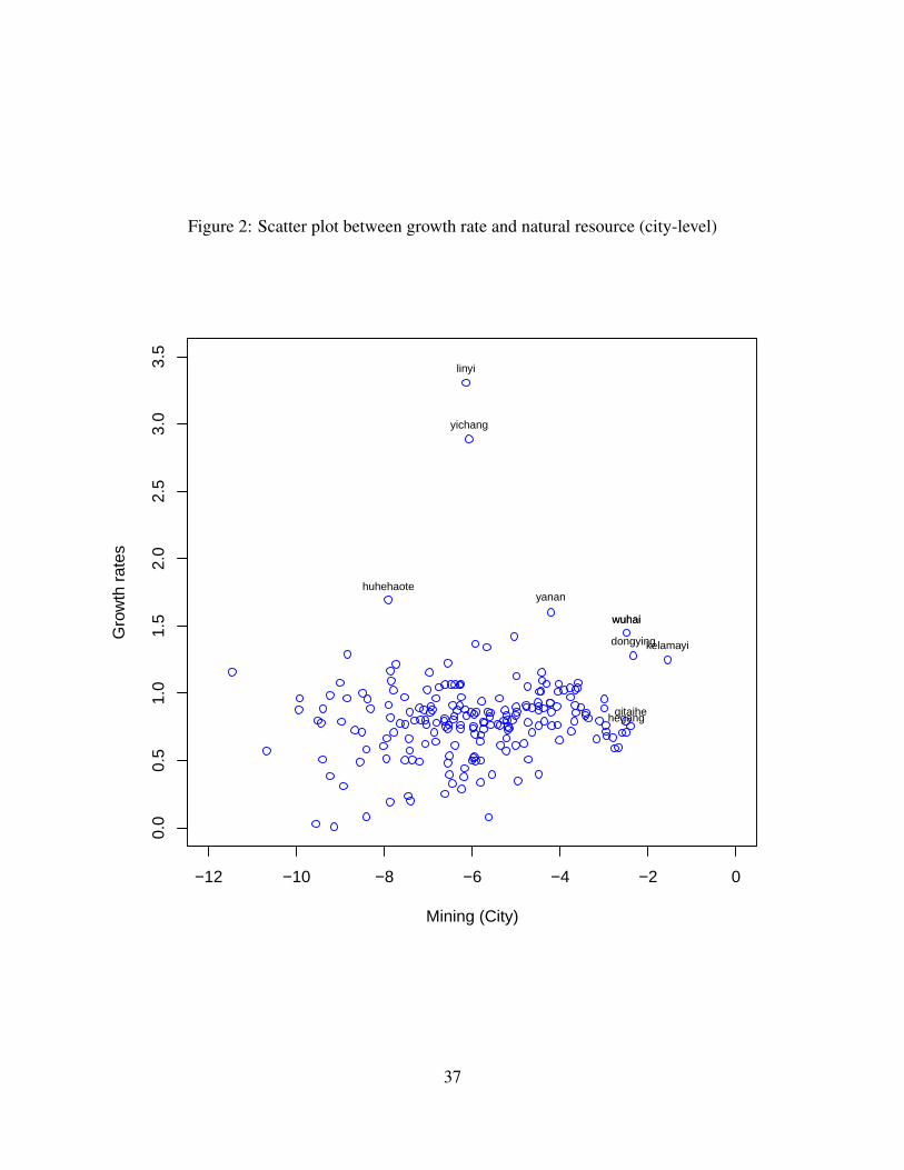
Figure 2: Scatter plot between growth rate and natural resource (city-level)

−12 −10 −8 −6 −4 −2 0

0.0

0.5

1.0

1.5

2.0

2.5

3.0

3.5

Mining (City)

Gro

wth

rat

es

hegang

wuhai

qitaihe

dongyingkelamayi

wuhai

yananhuhehaote

yichang

linyi

37

Figure 3: Scatter plot between growth rate and natural resource (rural-level)

−12 −10 −8 −6 −4 −2 0

0.0

0.5

1.0

1.5

2.0

Mining (Rural)

Gro

wth

rat

es

taiansanmenxia

jincheng

taiyuan

yichun

baotoubenxi

liupanshuiyingkouhuhehaote

38

Figure 4: Estimation results : initial GDP per capita level

−2.1 −1.9 −1.7

−0.

2−

0.1

0.0

0.1

0.2

GDP in 1990 (City)

log(manufacture)

coef

ficie

nt

−2.1 −1.9

−0.

2−

0.1

0.0

0.1

0.2

0.3

0.4

0.5

GDP in 1990 (Rural)

log(manufacture)

coef

ficie

nt

0.000 0.006 0.012

−0.

050.

050.

100.

150.

200.

250.

30

GDP in 1990 (City)

FDI

coef

ficie

nt

0.000 0.003 0.006

−0.

3−

0.2

−0.

10.

00.

10.

20.

3

GDP in 1990 (Rural)

FDI

coef

ficie

nt

−8.0 −7.0 −6.0 −5.0

−0.

3−

0.2

−0.

10.

00.

10.

20.

3

GDP in 1990 (City)

log(R&D)

coef

ficie

nt

−8.0 −7.0 −6.0

−0.

3−

0.2

−0.

10.

00.

10.

20.

3

GDP in 1990 (Rural)

log(R&D)

coef

ficie

nt

0.006 0.009

−0.

15−

0.05

0.05

0.10

0.15

0.20

GDP in 1990 (City)

Teacher

coef

ficie

nt

0.005 0.008 0.011

−0.

15−

0.10

−0.

050.

000.

05

GDP in 1990 (Rural)

Teacher

coef

ficie

nt

Notes: Solid and dotted lines represent estimated functional coefficients and 95% confidence bands, respectively.

39

Figure 5: Estimation results : mining

−2.1 −1.9 −1.7

−0.

15−

0.05

0.05

0.10

0.15

0.20

Mining (City)

log(manufacture)

coef

ficie

nt

−2.1 −1.9

−0.

050.

000.

050.

100.

150.

20

Mining (Rural)

log(manufacture)

coef

ficie

nt

0.000 0.006 0.012

−0.

10−

0.05

0.00

0.05

0.10

Mining (City)

FDI

coef

ficie

nt

0.000 0.003 0.006

−0.

20−

0.10

0.00

0.05

0.10

0.15

Mining (Rural)

FDI

coef

ficie

nt

−8.0 −7.0 −6.0 −5.0

−0.

2−

0.1

0.0

0.1

0.2

Mining (City)

log(R&D)

coef

ficie

nt

−8.0 −7.0 −6.0

−0.

2−

0.1

0.0

0.1

0.2

Mining (Rural)

log(R&D)

coef

ficie

nt

0.006 0.009

−0.

020.

000.

020.

040.

060.

080.

10

Mining (City)

Teacher

coef

ficie

nt

0.005 0.008 0.011

0.00

0.02

0.04

0.06

0.08

Mining (Rural)

Teacher

coef

ficie

nt


40

Figure 6: Estimation results : diffusion

−2.1 −1.9 −1.7

0.00

0.05

0.10

Diffusion (City)

log(manufacture)

coef

ficie

nt

−2.1 −1.9

−0.

020.

000.

020.

04

Diffusion (Rural)

log(manufacture)

coef

ficie

nt

0.000 0.006 0.012

−0.

020.

000.

020.

040.

060.

08

Diffusion (City)

FDI

coef

ficie

nt

0.000 0.003 0.006

−0.

020.

000.

020.

040.

06

Diffusion (Rural)

FDI

coef

ficie

nt

−8.0 −7.0 −6.0 −5.0

−0.

020.

000.

020.

040.

060.

080.

10

Diffusion (City)

log(R&D)

coef

ficie

nt

−8.0 −7.0 −6.0

−0.

06−

0.02

0.00

0.02

0.04

0.06

Diffusion (Rural)

log(R&D)

coef

ficie

nt

0.006 0.009

−0.

020.

000.

020.

04

Diffusion (City)

Teacher

coef

ficie

nt

0.005 0.008 0.011

−0.

02−

0.01

0.00

0.01

0.02

0.03

Diffusion (Rural)

Teacher

coef

ficie

nt


41

resource abundance and economic growth in...

Documents