This is a repository copy of Resolving Forward-Reverse Logistics Multi-Period Model: An Artificial Immune System Algorithm Based Approach.

White Rose Research Online URL for this paper:http://eprints.whiterose.ac.uk/100267/

Version: Accepted Version

Article:

Kumar, V.N.S.A, Kumar, V., Brady, M. et al. (2 more authors) (2017) Resolving Forward-Reverse Logistics Multi-Period Model: An Artificial Immune System Algorithm Based Approach. International Journal of Production Economics, 183 (B). pp. 458-469. ISSN 0925-5273

https://doi.org/10.1016/j.ijpe.2016.04.026

Article available under the terms of the CC-BY-NC-ND licence (https://creativecommons.org/licenses/by-nc-nd/4.0/)

eprints@whiterose.ac.ukhttps://eprints.whiterose.ac.uk/

Reuse

This article is distributed under the terms of the Creative Commons Attribution-NonCommercial-NoDerivs (CC BY-NC-ND) licence. This licence only allows you to download this work and share it with others as long as you credit the authors, but you can’t change the article in any way or use it commercially. More information and the full terms of the licence here: https://creativecommons.org/licenses/

Takedown

If you consider content in White Rose Research Online to be in breach of UK law, please notify us by emailing eprints@whiterose.ac.uk including the URL of the record and the reason for the withdrawal request.

Resolving Forward-Reverse Logistics Multi-Period Model Using Evolutionary

Algorithms

Abstract

In the changing competitive landscape and with growing environmental awareness, reverse

logistics issues have become prominent in manufacturing organizations. As a result there is an

increasing focus on green aspects of the supply chain to reduce environmental impacts and

ensure environmental efficiency. This is largely driven by changes made in government rules and

regulations with which organizations must comply in order to successfully operate in different

regions of the world. Therefore, manufacturing organizations are striving hard to implement

environmentally efficient supply chains while simultaneously maximizing their profit to compete

in the market. To address the issue, this research studies a forward-reverse logistics model. This

paper puts forward a model of a multi-period, multi-echelon, vehicle routing, forward-reverse

logistics system. The network considered in the model assumes a fixed number of suppliers,

facilities, distributors, customer zones, disassembly locations, re-distributors and second

customer zones. The demand levels at customer zones are assumed to be deterministic. The

objective of the paper is to maximize the total expected profit and also to obtain an efficient

route for the vehicle corresponding to an optimal/ near optimal solution. The proposed model is

resolved using Artificial Immune System (AIS) and Particle Swarm Optimization (PSO)

algorithms. The findings show that for the considered model, AIS works better than the PSO.

This information is important for a manufacturing organization engaged in reverse logistics

programs and in running units efficiently. This paper also contributes to the limited literature on

reverse logistics that considers costs and profit as well as vehicle route management.

Keywords: Reverse Logistics; Supply Chain; AIS; PSO; Vehicle Routing; Profit; Cost

1. Introduction

Supply chain management (SCM) has nowadays become a crucial strategy for firms to increase

their profitability and stay competitive (Li et al., 2006; Tan et al., 2002). Thus, over the last

decade, researchers and practitioners have increased the degree of attention paid to SCM. This

has resulted in a rich stream of research mainly focused on particular management aspects of

supply chains that include, among many others: supplier alliances (Lee et al., 2009; Kannan and

Tan, 2004), supplier selection (Ageron et al., 2013; Viswanadham and Samvedi, 2013), supplier

management (Reuter et al., 2010), involvement of suppliers (Johnsen, 2011), upstream supply

chain (SC) related research (Finne and Holmström, 2013; Oosterhuis et al., 2012), supply chain

resilience (Carvalho et al., 2014), manufacturer and retailers linkages (Li and Zhang, 2015; Zhao

et al., 2008) and SCM practices (Narasimhan and Schoenherr, 2012; Li et al., 2006; Li et al.,

2005). Traditionally, SCM research has concentrated on improving profitability, efficiency,

customer satisfaction, quality and responsiveness, which had been the dominant concern for

organisations (Green et al., 2012), However, in order to respond to governmental environmental

regulations and the growth of customer demands for products and services that are

environmentally sustainable, companies have now been forced to rethink how they manage their

supply chains to also consider the environmental dimension.

Evidence suggests that in order to support organizations to align with governmental regulations

and respond to the ‘environmental push’ of customers, academic research has also focused on the

recently emerged green aspect of SCM, particularly in the areas of sustainable supply chains

(Jabbour et al., 2015; Dadhich et al., 2015; Hassini et al., 2012), green supply chains (Kumar et

al., 2015; Bhattacharya et al., 2014; Green et al., 2012), circular economy supply chains

(Genovese et al., 2015; Pan et al., 2015; Ying and Li-jun, 2012) and reverse logistics

(Abdulrahman et al., 2014; García-Rodríguez et al. 2013; Mishra et al. 2012; Vishwa et al.,

2010). However, despite this relatively abundant research, many manufacturing organizations are

still struggling to implement environmentally efficient supply chains while simultaneously

maximizing profit while competing in the marketplace (Srivastava, 2007). There is limited

research focused on the cost of the whole supply chain including reverse logistics activities

(Srivastava, 2007; El-Sayed et al. 2010). To address this issue, this paper proposes a forward-

reverse logistics model, in particular, a model for a multi-period, multi -echelon, vehicle routing,

forward-reverse logistics system to maximize the total expected profit and also to obtain an

efficient route for the vehicle corresponding to an optimal/ near optimal solution. The proposed

model is resolved using an evolutionary Artificial Immune System (AIS) algorithm.

The remainder of the paper is organised as follows: Section 2 provides a review on reverse

logistics to serve as a preamble for the development of the forward-reverse logistics model

proposed; the model is then introduced in Section 3 and algorithm is described in Section 4;

Section 5 discusses the findings of this study and Section 6 presents the conclusions.

2. Literature Review

2.1 Emergence of Reverse Logistics

Environmental issues were largely ignored by manufacturing firms until they were forced by

government agencies and regulations to implement environmentally friendly methods to reduce

the CO2 emissions generated by their supply chains, production systems and practices. This led

to the emergence of ‘sub-areas’ in the field of supply chain management that included green

supply chains (Mohanty and Prakash, 2014; Zhu et al., 2008), green logistics (Ubeda et al.,

2011) and reverse logistics (Mishra et al., 2012; Sarkis, 2003; Huang et al., 2012). These sub-

areas have nowadays become of prime interest to researchers and practitioners around the world.

Reverse logistics gained momentum since the mid-nineties especially with legal enforcement of

product and material recovery or disposal both in Europe and in the US. Despite its emergence in

early to mid-nineties Dowlatshahi (2000) reported that there was a lack of theory development in

the area of reverse logistics. As a result over the past decade a number of papers have been

published addressing various problems surrounding reverse logistics operations in different

industrial settings (Choudhary et al. 2015; Abdulrahman et al., 2014; García-Rodríguez et al.

2013; Huang et al., 2012; Mishra et al. 2012; Vishwa et al. 2010; Sarkis 2003). De Brito and

Dekker (2002) presented a comprehensive review of reverse logistics literature and definitions.

In addition, they presented a decision framework for reverse logistics based on a long, medium

and short term perspective. Following de Brito and Dekker’s (2002) work several other

researchers discussed the evolution of reverse logistics and highlighted the significance of

reverse logistics operations to manufacturing organisations (Ko and Evans, 2007; Mishra et al.

2012; Wang et al., 2012). A review of recent research shows that reverse logistics is still

attracting much interest, however the direction of research is now moving towards incorporating

sustainability (Sarkis et al., 2010; Brix-Asala et al., 2016) and circular economy concepts in

conjunction with reverse logistics (Meng, 2013; Chen et al., 2015). The next section provides a

brief overview of reverse logistics definitions.

2.2 Definitions

With the increasing worldwide importance of green supply chains much research work has been

carried out both in the forward logistics part of the supply chain as well as in reverse logistics

(Ko and Evans, 2007; de la Fuente, 2008; El-Sayed et al., 2010; Pishvaee, Farahani, & Dullaert,

2010). Several researchers have put forward definitions of reverse logistics: Kroon and Vrijens

(1994) referred to reverse logistics as the logistic management skills and activities involved in

reducing, managing and disposing of hazardous and non-hazardous waste from packaging and

products. Dowlatshahi (2000) defined reverse logistics as the process by which the manufacturer

systematically accepts previously shipped products or parts from the point of consumption for

possible recycling, remanufacturing or disposal. Rogers and Tibben-Lembke (1999) similarly

defined reverse logistics as the process of planning, implementing and controlling the efficient,

cost effective flow of raw materials, in-process inventory, finished goods and related information

from the point of consumption to the point of origin for the purpose of recapturing value, or

proper disposal. This definition was further modified by De Brito and Dekkar (2002) who

emphasized the point of recovery rather than the point of origin. These definitions show a broad

agreement on the main elements of reverse logistics.

2.3 Previous Research

Research in the field of reverse logistics has been primarily centered on studying its benefits,

determining the barriers that organizations face when implementing a reverse approach to their

logistics operations, and essential elements (e.g. vehicle routing and cost) that comprise these

operations. For example, recent research by Abdulrahman et al. (2014) focused on identifying

the barriers of reverse logistics operations in the Chinese manufacturing sector. Their study

identified as barriers: a lack of reverse logistics experts and low commitment, a lack of initial

capital and funds for return monitoring systems, a lack of enforceable laws and lack of

supportive government economic policies and, finally, a lack of systems for return monitoring.

García-Rodríguez et al. (2013) showed that application of reverse logistics can be beneficial in

acquiring raw materials in developing countries as it can reduce the problem of acquisition of

production inputs and mitigate environmental damage caused by the production of raw materials.

A number of researchers have also investigated vehicle routing problem in reverse logistics

operations (Dethloff, 2001; El-Sayed et al., 2010; Shukla et al., 2013; Tiwari and Chang, 2015;

Soysal et al., 2015; Kim and Lee, 2015). Since vehicle routing is an essential element of reverse

logistics operations, it is important that manufacturing organizations manage this efficiently. As

indicated earlier, several researchers have attempted to optimize vehicle routing operations but

studies simultaneously focused combining this with maximizing profit still remain scant

(Srivastava, 2007; El-Sayed et la. 2010; Soysal et al. 2015). Thus, this paper aims to address this

research gap and add to the existing knowledge and understanding in this area.

Green distribution and marketing involves efficient route planning and fuel reduction as well as

the promotion of eco-friendly products. Reverse logistics aims at the strict supervision and

efficient management of waste materials. Fleischmann et al. (1997) presented quantitative

models for reverse logistics and suggested key areas of research in distribution planning,

inventory control, and production planning. Ravi et al. (2008), in their study of key issues

involved in the environmentally friendly disposal of end-of-life (EOL) computers, proposed a

hybrid approach comprising analytical network process (ANP) and zero one goal programming

(ZOGP) to select the reverse logistics projects. Teunter (2001) proposed a reverse logistics

valuation model for inventory control and argued that the proposed method is 'correct' from a

discounted cash flow (DCF) point of view. The role of JIT in a reverse logistics model was

studied by Chan et al. (2010) who found that a process model with JIT improves cost control,

efficiency of reverse logistics activities as well as the product life cycle management. More

recently Tiwari and Chang (2015) proposed a block recombination approach to solve the green

vehicle routing problem. Their study primarily aimed at minimizing carbon dioxide emissions by

vehicle during the transportation of goods from depot to customer while minimizing total

distance travelled by the vehicle. These studies show that routing planning has been high on the

agenda of researchers focusing on improving reverse logistics operations.

2.3.1 Reverse Logistics Costs

There are many costs involved in reverse logistics operations similar to those of forward logistics

operations. Dowlatshahi (2000) emphasizes that firms should establish a cost and benefits

structure for its reverse logistics system and should consider the operational costs, land fill and

contingent liability costs. Dowlatshahi (2010) later explored the role of inbound and outbound

transportation within the context of a reverse logistics (RL) system and puts forward eight

propositions marking the importance of the transport system in reverse logistic operations. One

of these propositions is related to transportation cost which proposes that the effectiveness of a

transportation system in RL is positively related to the use of cost-efficient transportation rates.

Bachlaus et al. (2008) designed a multi-echelon agile supply chain network with the aim of

minimizing cost and maximizing plant flexibility and volume flexibility to increase the

profitability of a manufacturing firm. Tsai and Hung (2009) studied the reverse logistics problem

of waste electrical and electronic equipment (WEEE) focusing on treatment and recycling system

optimization. They considered activity-based costing as a tool in WEEE reverse logistics

management and proposed a concise supply-chain decision framework with producer

responsibility. Weeks et al. (2010) carried out an empirical investigation to understand the

impact of the product mix and product route efficiencies on operations performance and

profitability. Their findings showed that operations management alone does not have a positive

impact on profitability; rather it is the production mix efficiency and product route efficiency

together that have a positive effect on profitability. More recently, Soysal et al. (2015) presented

a multi-period inventory routing model that included load dependent distribution costs for a

comprehensive evaluation of CO2 emission and fuel consumption, perishability, and a service

level constraint for meeting uncertain demand. Their proposed integrated model showed

significant savings in total cost while satisfying the service level requirements and thus offering

better support to decision makers. These studies highlight the significance of cost related issues

in the overall success of a reverse logistics model.

2.3.2 Cost Optimization

Many researchers have presented algorithms to find a path by which costs associated with the

supply chain can be minimized. As simultaneous delivery and pickup activities are preferred by

customers, this aspect is considered by Dethloff (2001) as a vehicle routing problem with

simultaneous delivery and pick-up (VRPSDP). Choudhary et al. (2015) proposed a quantitative

optimization model for integrated forward–reverse logistics with carbon-footprint considerations.

They implemented a modified and efficient forest data structure to derive the optimal network

configuration, minimizing both the cost and the total carbon footprint of the network. Their

proposed method outperformed the conventional genetic algorithm (GA) for large problem sizes.

Zheng and Zhang (2008) proposed a genetic algorithm to solve a vehicle routing problem with

simultaneous pickup and delivery. Ko and Evans (2007) also applied a genetic algorithm-based

heuristic for the dynamic integrated forward/reverse logistics network for third party logistics

providers. They compared their solutions to optimal solutions using different test problems to

show the efficacy of the evolutionary algorithm in resolving reverse logistics problems.

Pishvaee, Farahani, & Dullaert (2010) proposed a memetic algorithm for bi-objective integrated

forward/reverse logistics network design model. Their proposed algorithm outperformed the

existing multi-objective genetic algorithm. A stochastic mixed integer linear programming model

was put forward by El-Sayed et al. (2010) to solve forward-reverse logistics problems with the

objective of maximizing total expected profit. These studies show that a variety of algorithms

have been applied by researchers to resolve reverse logistics issues. In this paper El-Sayed et

al.’s (2010) model is modified to include the importance of vehicle routing in a reverse logistics

scenario and is solved using Artificial Immune System (AIS) and Particle Swarm Optimization

(PSO) evolutionary algorithms.

Srivastava (2007) reviewed the literature on green supply chain management and observed that

much research has been focused on delivering product to end customers at lower supply chain

cost but limited research has been carried out on the cost of the whole supply chain including

reverse logistics activities. For example, Kheljani et al., (2009) attempted to optimize the total

cost of the supply chain rather than only the buyer's cost. However, the total cost of their supply

chain includes only buyer's cost and suppliers’ costs. Pettersson and Segerstedt (2013) following

the same line focused on measuring the Supply Chain Cost (SCC), and this study too did not take

in to account the reverse logistics costs which show the gap that exists in the literature. We

therefore aim to fill this research gap and contribute in this domain.

Given that customers generally do not prefer delivery and pickup activities separately but prefer

them to be carried out simultaneously, we suggest that there should be some fixed route for a

vehicle, given a fixed number of agents in the supply chain, by which costs for the entire chain

can be optimized. In the remainder of the paper we put forward a model whereby total expected

profit of a forward-reverse logistic situation is maximized and where the route that a vehicle

should follow is determined using an AIS clonal-selection algorithm. The upcoming sections

discuss the AIS algorithm more in detail.

3. Model Description

The model proposed in this study is a modification of and extension to the forward-reverse

logistics network design problem proposed by El-Sayed et al. (2010). However, our proposed

model is different from El-Sayed et al.’s (2010) work in a number of ways. As compared to El-

Sayed et al.'s (2010) work, the major contribution of our paper is the integration of vehicle

routing into modified (as compared to earlier model) network structure of forward-reverse

logistics network. The flow in our model has also been modified by including recycling and

repair center to handle repair parts. In addition, our study considers vehicle routing (path) integer

variable as a constraint to get transportation path for the model.

The network is multi-period and multi-echelon, and consists of suppliers, facilities, distributors

and first customers and in the forward direction and in the reverse direction it consists of

disassembly, disposal, recycling locations, redistribution locations and second customers. The

objective of the paper is to maximize profit in a reverse logistics environment while considering

vehicle constraints and minimizing the cost of transportation.

The model considers a company which has a fixed number of locations for each type of agent in

the supply chain. We consider two suppliers, two distributors and three customer zones, and one

each of the remaining agents: facility, facility store, disassembly location, disposal center,

recycling center, redistribution location and second customer zone. The company has one vehicle

which every period goes from the transport depot to collect and deliver goods from one location

to the other.

3.1 Network Flows

The facility receives raw materials from the suppliers and goods manufactured at the facility will

be stored in the facility store after every period. Distributors receive goods either directly from

the facility or from the facility store. The distributors service the customers according to the

demand. Used goods are collected from customers and shipped to the disassembly location.

Here, goods are sorted and sent to the recycling and repair center. Goods for disposal are sent to

the disposal location and repaired and recycled goods are sent to respective locations: goods to

be remanufactured are sent to the facility; repaired goods to the redistribution centre and recycled

goods to the facility from which they enter the supply chain again as raw materials. The

redistribution center in turn receives remanufactured goods from the facility and repaired goods

from the recycling and repair center. These used products after repairing and remanufacturing are

sold to secondary customers according to demand. These are usually sold at low prices compared

to fresh goods. An example for such a model is given in Figure 1.

[Insert Figure 1 here]

Costs considered at different nodes of the model are as follows:

1) Suppliers: These include material costs and transportation costs.

2) Facilities: These include manufacturing costs, remanufacturing costs, storage costs and

transportation costs.

3) Facility store: These include holding costs and transportation costs.

4) Distributors: These include shortage costs, storage costs and transportation costs.

5) Disassembly locations: These include costs for disassembly operations, inspection and

sorting costs, repairing costs and transportation costs.

6) Recycling Center: These include costs for recycling of materials.

7) Redistribution Centers: These include costs for transportation.

8) Disposal Locations: These include disposal costs and transportation costs.

3.2 Model Assumptions

The following are the major assumptions made with respect to the model:

1) The model is multi-period and multi-echelon.

2) The locations of the chain are fixed and the number of each location is given.

3) Cost parameters are known for each location and time period.

4) The demand quantities at first customer zone are known.

5) Capacity of each location is not limited.

6) The holding cost depends on the residual inventory at the end of period.

7) The path considered for the model is in the order: depot, supplier, facility, facility store,

distributor, first customer zone, disassembly location, recycling center, facility,

redistributors, and second customer.

8) The disposal center is assumed to be near to the disassembly location.

3.3 Model Formulation

3.3.1 Decision Variables

Q(d)(c)(t) – flow of goods from distributor(d) to first customer(c) in period ‘t’

Q(d1)(c2)(t) –.flow of goods from re-distributor(d1) to second customer(c2) in period ‘t’

Q(s)(f)(t) – flow of goods from supplier(s) to facility(f) in period ‘t’

Q(f)(d)(t) – flow of goods from facility(f) to distributor(d) in period ‘t’

Q(f1)(d)(t) – flow of goods from facility store (f1) to distributor(d) in period ‘t’

Q(l)(r1)(t) – flow of goods from disassembly location(l) to recycling center(r1) in period ‘t’

Q(f)(r1)(t) – flow of goods from facility(f) to recycling center(r1) in period ‘t’

Q(r1)(d1)(t) – flow of goods from recycling center(r1) to re-distributor center(d1) in period ‘t’

Q(c)(l)(t) – flow of goods from first customer(c) to disassembly location(l) in period ‘t’

Q(c)(r1)(t) – flow of goods first customer(c) to recycling center(r1) in period ‘t’

Q(l)(g)(t) – flow of goods from disassembly location(l) to disposal location(g) in period ‘t’

Qrm(l)(f)(t) – flow of goods from disassembly location(l) to facility(f) in period 't'

Qrd(l)(r1)(t) – flow of goods from disassembly location(l) to recycling center(r1) in period 't'

Qrd(l)(d1)(t) – flow of goods from disassembly location(l) to re-distributor center(d1) in period 't'

Qrd(r1)(d1)(t) – flow of goods to recycling center(r1) to re-distributor center(d1) in period 't'

Qrc(r1)(f)(t) – flow of goods from recycling center(r1) to facility(f) in period 't'

Qrc(r1)(d1)(t) – flow of goods from recycling center(r1) to re-distributor center(d1) in period 't'

I(f)(f1)(t) – flow of goods from facility(f) to store(f1) in period 't'

I(f1)(d)(t) – flow of goods from facility store(f1) to distributor location(d) in period 't'

R(f1)(t) – residual inventory at facility store(f1) in period ‘t’

R(d)(t) – residual inventory at distributor location(d) in period 't'

x(i)(j) – binary variable = 1 if vehicle take goes from location 'i' to location 'j'

= 0 if vehicle doesn’t take that path.

3.3.2 Symbols

T1 – Number of Transport Depots

S – Number of Suppliers

F – Number of Facilities

F1 – Number of Facility Stores

D – Number of Distributors

C1– Number of Primary Customers

L – Number of Disassembly Locations

R1–Number of Recycling and Repair Centers

G – Number of Disposal Locations

D1 – Number of Redistributing Locations

C2 – Number of Secondary Customers

T – Total number of time periods

N– Total number of Locations

MC – Material cost per unit supplied by supplier

RC – Recycling cost per unit recycled

FC – Manufacturing cost per unit manufactured

FH –Inventory holding cost per unit at facility store

PC – Purchasing cost (for recycling) per unit

SC – Shortage cost per unit per period

DAC – Disassembly cost per unit disassembled

RMC – Remanufacturing cost per unit remanufactured

RDC – Repairing cost per unit repaired

DC – Disposal cost per unit disposed

DH – Holding cost per unit per period at distribution location

P(c)t – Unit price at first customer c in period t

P(c2)t – Unit price at second customer c2 in period t

D(c}(t) – Demand of first customer c in period t

D(c2}(t) – Demand of second customer c2 in period t

C(i)(j) – Transportation cost from moving from location 'i' to location 'j'

RR – Returning ratio at first customer

RM – Remanufacturing ratio

Rd – Redistribution ratio

RD – Disposal ratio

Rc – Recycling ratio

3.3.3 Objective Function

The objective is to maximize the total expected profit and to determine the path of the vehicle

corresponding to that level of profit.

Total Expected Profit = Total expected income – Total expected cost

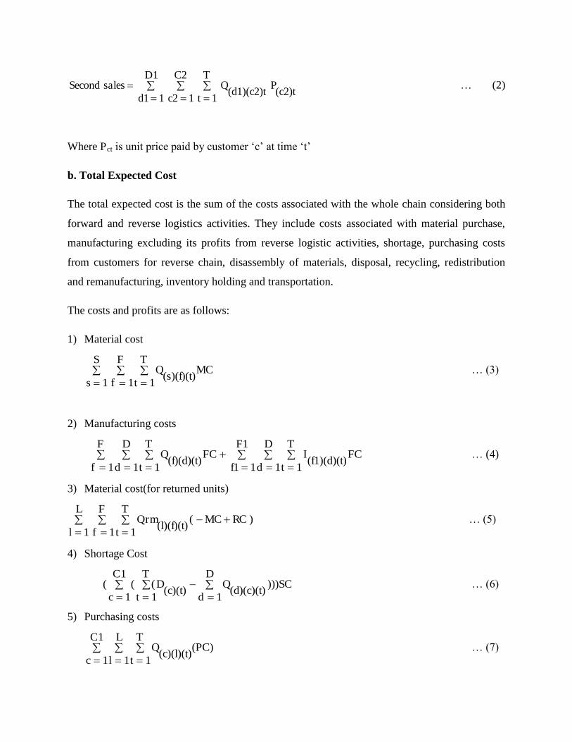
a. Total Expected Income

Total expected income = first sales + second sales

(c)t

PD

1d

C1

1c

T

1t

(d)(c)tQ salesFirst

…(1)

(c2)t

P D1

1d1

C2

1c2

T

1t(d1)(c2)t

Q salesSecond

… (2)

Where Pct is unit price paid by customer ‘c’ at time ‘t’

b. Total Expected Cost

The total expected cost is the sum of the costs associated with the whole chain considering both

forward and reverse logistics activities. They include costs associated with material purchase,

manufacturing excluding its profits from reverse logistic activities, shortage, purchasing costs

from customers for reverse chain, disassembly of materials, disposal, recycling, redistribution

and remanufacturing, inventory holding and transportation.

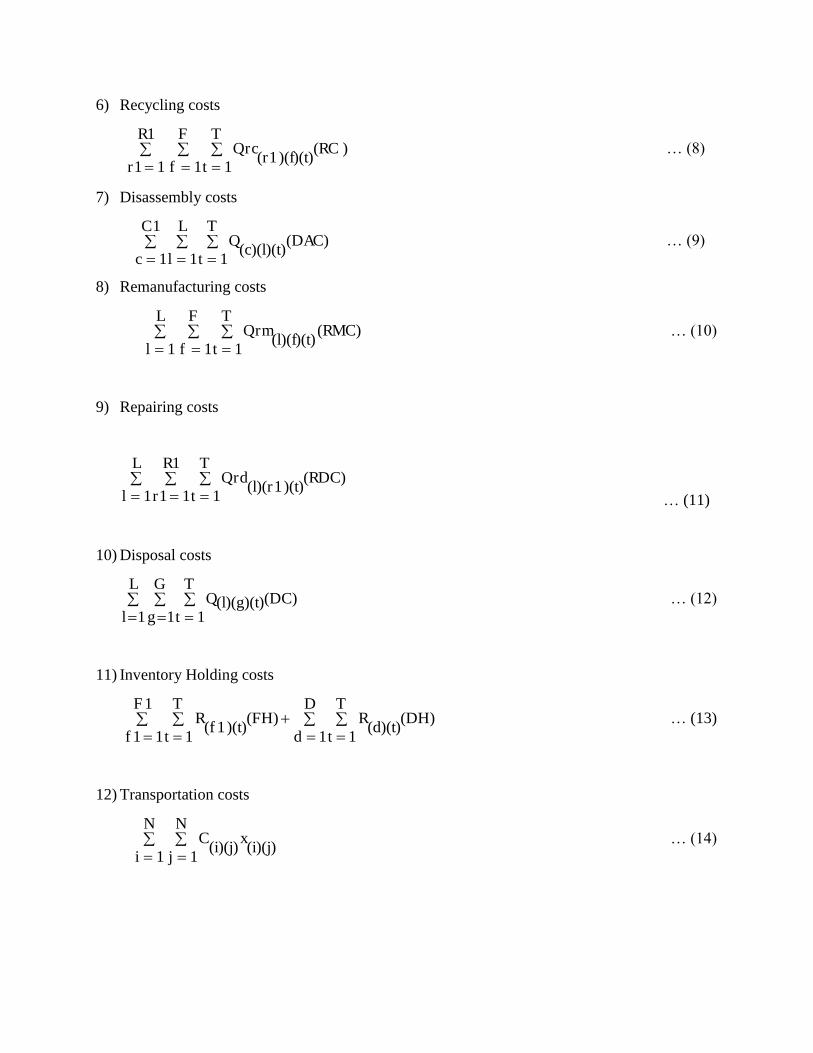
The costs and profits are as follows:

1) Material cost

MCS

1s

F

1f

T

1t(s)(f)(t)

Q

… (3)

2) Manufacturing costs

F1

1f1 FC

D

1d

T

1t(f1)(d)(t)

IF

1fFC

D

1d

T

1t(f)(d)(t)

Q

… (4)

3) Material cost(for returned units)

)RCMCL

1l

F

1f

T

1t(

(l)(f)(t)Qrm

… (5)

4) Shortage Cost

)))SCD

1d(d)(c)(t)

Q(c)(t)

D1C

1c

T

1t(( (

… (6)

5) Purchasing costs

(PC)1C

1c

L

1l

T

1t(c)(l)(t)

Q

… (7)

6) Recycling costs

R1

1r1

F

1f )(RC

T

1t)(f)(t)1(r

Qrc

… (8)

7) Disassembly costs

(DAC)1C

1c

L

1l

T

1t(c)(l)(t)

Q

… (9)

8) Remanufacturing costs

(RMC)L

1l

F

1f

T

1t(l)(f)(t)

Qrm

… (10)

9) Repairing costs

L

1l

R1

1r1 (RDC)

T

1t)(t)1(l)(r

Qrd

… (11)

10) Disposal costs

L

1l

G

1g (DC)

T

1t(l)(g)(t)Q

… (12)

11) Inventory Holding costs

(DH)D

1d

T

1t(d)(t)

R1F

11f(FH)

T

1t)(t)1(f

R

… (13)

12) Transportation costs

(i)(j)

xN

1i

N

1j(i)(j)

C

… (14)

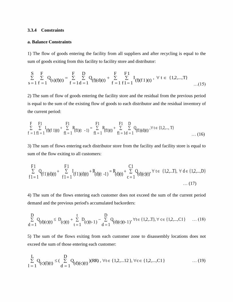
3.3.4 Constraints

a. Balance Constraints

1) The flow of goods entering the facility from all suppliers and after recycling is equal to the

sum of goods exiting from this facility to facility store and distributor:

T} ,...,2,1 { t , F

1f

1F

11f)(t)1(f)(f

IF

1f

D

1d(f)(d)(t)

QS

1s

F

1f(s)(f)(t)

Q

…(15)

2) The sum of flow of goods entering the facility store and the residual from the previous period

is equal to the sum of the existing flow of goods to each distributor and the residual inventory of

the current period:

T} {1,2,...,t ,F1

1f1

D

1d(f1)(d)(t)

QF1

1f1(f1)(t)

R F1

1f11)- (f1)(t

RF

1f

F1

1f11)(t) (f)(f

I

… (16)

3) The sum of flows entering each distributor store from the facility and facility store is equal to

sum of the flow exiting to all customers:

D},...,2,1{ dT}, ,...2,1 { t, 1C

1c(d)(c)(t)

Q(d)(t)

R)1- (d)(t

R1F

11f)(d)(t)1(f

I 1F

11f)(d)(t)1(f

Q

… (17)

4) The sum of the flows entering each customer does not exceed the sum of the current period

demand and the previous period's accumulated backorders:

}1C,...,2,1{ cT}, ,..2,1{t, D

1d)1 (d)(c)(t-

Qt

1t)1 (c)(t-

D(c)(t)

DD

1d(d)(c)(t)

Q

… (18)

5) The sum of the flows exiting from each customer zone to disassembly locations does not

exceed the sum of those entering each customer:

}1C,...,2,1{c}, 12,...2,1{t)(RR) , D

1d(d)(c)(t)

Q(L

1l(c)(l)(t)

Q

… (19)

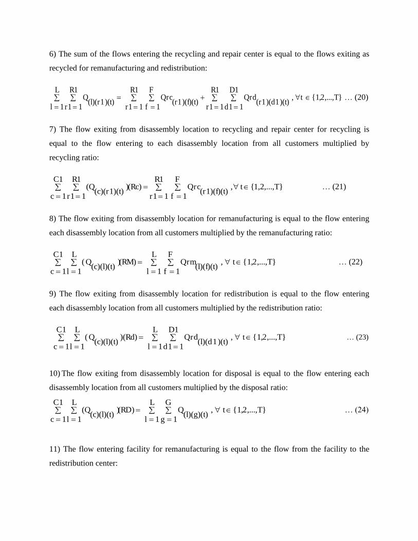
6) The sum of the flows entering the recycling and repair center is equal to the flows exiting as

recycled for remanufacturing and redistribution:

T},...,2,1{t , 1R

11r

1D

11d)(t)1)(d1(r

Qrd1R

11r

F

1f)(f)(t)1(r

Qrc L

1l

1R

11r)(t)1(l)(r

Q

… (20)

7) The flow exiting from disassembly location to recycling and repair center for recycling is

equal to the flow entering to each disassembly location from all customers multiplied by

recycling ratio:

T}{1,2,...,t ,R1

1r1

F

1f(r1)(f)(t)

Qrc (Rc)C1

1c

R1

1r1)

(c)(r1)(t)(Q

… (21)

8) The flow exiting from disassembly location for remanufacturing is equal to the flow entering

each disassembly location from all customers multiplied by the remanufacturing ratio:

T},...,2,1{ t , L

1l

F

1f(l)(f)(t)

Qrm (RM)1C

1c)

L

1l(c)(l)(t)

Q(

… (22)

9) The flow exiting from disassembly location for redistribution is equal to the flow entering

each disassembly location from all customers multiplied by the redistribution ratio:

T},...,2,1{ t , L

1l

1D

11d)(t)1(l)(d

Qrd )(Rd)1C

1c

L

1l(c)(l)(t)

Q(

… (23)

10) The flow exiting from disassembly location for disposal is equal to the flow entering each

disassembly location from all customers multiplied by the disposal ratio:

T},...,2,1{ t , L

1l

G

1g(l)(g)(t)

Q (RD)1C

1c

L

1l)

(c)(l)(t)(Q

… (24)

11) The flow entering facility for remanufacturing is equal to the flow from the facility to the

redistribution center:

T},...,2,1{ t , F

1f

1R

11r)(t)1(f)(r

Q L

1l

F

1f(l)(f)(t)

Qrm

… (25)

12) The flow entering redistribution center from the facility, recycling and the repair center is

equal to the flow exiting from it to the second customer:

T},...,2,1{ t, 1D

11d

2C

12c)(t)2)(c1(d

Q1R

11r

1D

11d)(t)1)(d1(r

Q F

1f

1R

11r)(t)1(f)(r

Q

… (26)

13) The flow entering the second customer zone from the redistribution center does not exceed

the second customer demand for a particular period:

}2C,..,2,1{ c2 ,T},..2,1{ t, )(t)2(c

D1D

11d)(t)2)(c1(d

Q … (27)

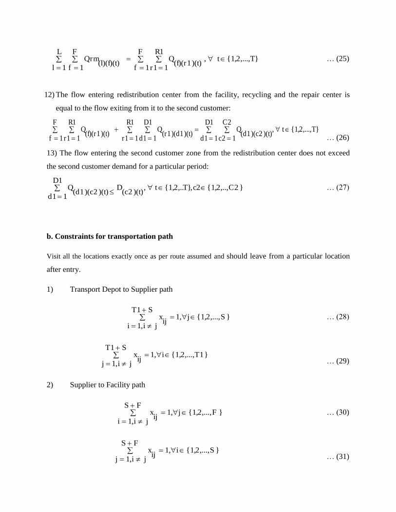
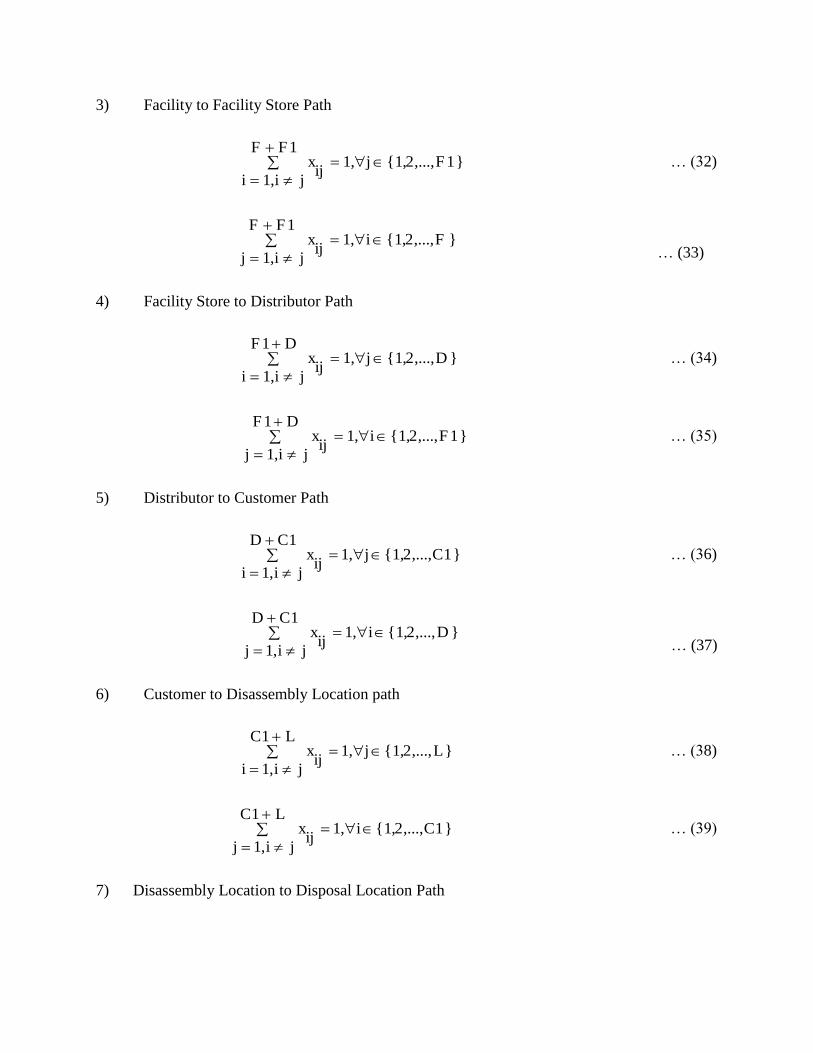
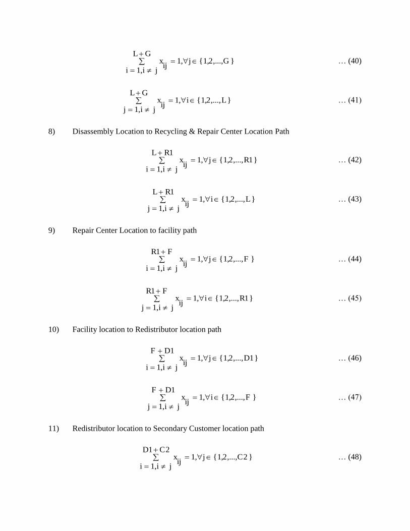
b. Constraints for transportation path

Visit all the locations exactly once as per route assumed and should leave from a particular location

after entry.

1) Transport Depot to Supplier path

}S,...,2,1{j,1S1T

ji,1iij

x

… (28)

}1T,...,2,1{i,1S1T

ji,1jij

x

… (29)

2) Supplier to Facility path

}F,...,2,1{j,1

FS

ji,1iij

x

… (30)

}S,...,2,1{i,1FS

ji,1jij

x

… (31)

3) Facility to Facility Store Path

}1F,...,2,1{j,11FF

ji,1iij

x

… (32)

}F,...,2,1{i,11FF

ji,1jij

x

… (33)

4) Facility Store to Distributor Path

}D,...,2,1{j,1

D1F

ji,1iij

x

… (34)

}1F,...,2,1{i,1D1F

ji,1jij

x

… (35)

5) Distributor to Customer Path

}1C,...,2,1{j,11CD

ji,1iij

x

… (36)

}D,...,2,1{i,1

1CD

ji,1jij

x

… (37)

6) Customer to Disassembly Location path

}L,...,2,1{j,1L1C

ji,1iij

x

… (38)

}1C,...,2,1{i,1L1C

ji,1jij

x

… (39)

7) Disassembly Location to Disposal Location Path

}G,...,2,1{j,1GL

ji,1iij

x

… (40)

}L,...,2,1{i,1

GL

ji,1jij

x

… (41)

8) Disassembly Location to Recycling & Repair Center Location Path

}1R,...,2,1{j,11RL

ji,1iij

x

… (42)

}L,...,2,1{i,1

1RL

ji,1jij

x

… (43)

9) Repair Center Location to facility path

}F,...,2,1{j,1F1R

ji,1iij

x

… (44)

}1R,...,2,1{i,1F1R

ji,1jij

x

… (45)

10) Facility location to Redistributor location path

}1D,...,2,1{j,11DF

ji,1iij

x

… (46)

}F,...,2,1{i,1

1DF

ji,1jij

x

… (47)

11) Redistributor location to Secondary Customer location path

}2C,...,2,1{j,12C1D

ji,1iij

x

… (48)

}1D,...,2,1{i,1

2C1D

ji,1jij

x

… (49)

The next section provides an overview of the algorithms in detail.

4. Algorithm Description

Solving the proposed model using conventional combinatorial techniques would be very difficult

and hence this study aims to use evolutionary techniques to solve the model. Evolutionary

techniques are known for resolving NP-hard combinatorial problems. Two popular evolutionary

algorithms Artificial Immune System (AIS) and Particle Swarm Optimization (PSO) were

applied to find solutions to the proposed model. We intend to compare the performance of these

two algorithms in resolving the model, and seek to investigate which algorithm can solve the

model in a lesser time. The upcoming section provides an overview of the two algorithms in

detail.

4.1 Artificial Immune System (AIS) Algorithm

Algorithms play an important role in resolving complex mathematical problems in operations

research. Over the years a number of algorithms have been proposed and applied to a wide range

of industrial problems. Nature has always inspired researchers and this inspiration and

understanding have led to the development of number of nature inspired algorithms, also known

as evolutionary algorithms that have been used to resolve complex optimization problems.

Among these are: Genetic Algorithms (GA), Ant Colony Optimization Algorithms (ACO),

Particle Swarm Optimization (PSO), Bee Colony Optimization (BCO) and Artificial Immune

System (AIS) based algorithms (Kennedy, 2010; Kumar et al., 2011; Moslehi and Mahnam,

2011). Each algorithm is inspired by a different natural activity, for example the Particle Swarm

Optimization Algorithm (Kennedy, 2010) emulates the real behavior of flocks of birds whereas

Bee Colony Optimization (Teodorović et al., 2006) is inspired by the way in which bees in

nature search for food. For large supply chain problems, classical optimization techniques such

as mixed integer linear programming might face oscillatory problems leading to a slower

solution time. However, evolutionary algorithms have been quite successful in resolving

complex optimization problems (Shahsavar, Najafi, & Niaki, 2015; Chiang and Lin, 2013; Ko

and Evans, 2007; Chan et al., 2006). In this paper, a comparison study has been performed

between Artificial Immune System and Particle Swarm Optimization to solve the logistics

problem considered in this paper.

The Artificial Immune System (AIS) algorithm, inspired by nature’s biological immune system

was proposed by De Castro et al. (2001; 2002). The prime function of an immune system is to

protect the body from unfamiliar invaders. To accomplish this task the body produces a number

of antigenic receptors that combat the attacking antigens. The cells that belong to our body and

which are harmless, are termed Self Antigens whereas, the disease causing cells are referred to as

Nonself Antigens (Kumar et al., 2006; Chan et al., 2006). The cells and molecules of the

immune system maintain constant surveillance for infecting organisms. They recognize an

almost limitless variety of infectious cells and substances distinguishing them from native

noninfectious cells. When a pathogen enters the body it is detected and mobilized for

elimination. The system is capable of remembering each infection so that a second exposure to

the same pathogen is dealt with more efficiently (Janeway, 1992). Based on this theory

algorithms are developed which can be used to tackle problems of pattern recognition, memory

acquisition and optimization.

CLONALG was developed to perform pattern recognition and optimization (De Castro et al.,

2001; White and Garrett, 2003; Diana et al., 2015; Pérez-Cáceres and Riff, 2015). This specific

algorithm is presented in this paper. The elements that can be detected by the immune system are

termed Antigens (Ag’s). To counter these, our body produces a number of antigenic receptors

that fight against attacking antigens. These molecules that protect the body from the foreign

invaders are known as Antibodies (Ab's). When an antigen is noticed the antibody, produced

from the B-Lymphocytes, which recognize an antigen will grow by cloning. In AIS, ‘Ag’s’ are

the optimal points of an objective function, while ‘Ab’s’ are the test configurations. The

optimization search is carried out by modifying ‘Abs’ in order to have a better affinity that yields

a greater value of the objective function. The next subsection shows the pseudo code of the

algorithm.

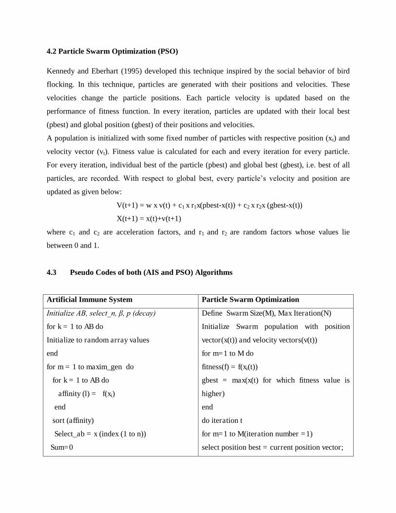
4.2 Particle Swarm Optimization (PSO)

Kennedy and Eberhart (1995) developed this technique inspired by the social behavior of bird

flocking. In this technique, particles are generated with their positions and velocities. These

velocities change the particle positions. Each particle velocity is updated based on the

performance of fitness function. In every iteration, particles are updated with their local best

(pbest) and global position (gbest) of their positions and velocities.

A population is initialized with some fixed number of particles with respective position (xt) and

velocity vector (vt). Fitness value is calculated for each and every iteration for every particle.

For every iteration, individual best of the particle (pbest) and global best (gbest), i.e. best of all

particles, are recorded. With respect to global best, every particle’s velocity and position are

updated as given below:

V(t+1) = w x v(t) + c1 x r1x(pbest-x(t)) + c2 x r2x (gbest-x(t))

X(t+1) = x(t)+v(t+1)

where c1 and c2 are acceleration factors, and r1 and r2 are random factors whose values lie

between 0 and 1.

4.3 Pseudo Codes of both (AIS and PSO) Algorithms

Artificial Immune System Particle Swarm Optimization

Initialize AB, select_n, く, p (decay)

for k = 1 to AB do

Initialize to random array values

end

for m = 1 to maxim_gen do

for k = 1 to AB do

affinity (l) = f(xi)

end

sort (affinity)

Select_ab = x (index (1 to n))

Sum=0

Define Swarm Size(M), Max Iteration(N)

Initialize Swarm population with position

vector(x(t)) and velocity vectors(v(t))

for m=1 to M do

fitness(f) = f(xi(t))

gbest = max(x(t) for which fitness value is

higher)

end

do iteration t

for m=1 to M(iteration number =1)

select position best = current position vector;

for k = 1 to_n do

NC(k) = round (く* AB/k)

for l = 1 to NC(k) do

MC(sum+) = Select_ab (k)+

exp(p)*tan(random term )

Affinity_MC(sum+l)= f(MC(sum+l))

end

sum=sum+NC(k)

end

In AB, last d antibodies are replaced with

new mutated child

end

Result = f (sort (AB (1)))

global best = position vector(gbest)

end

for m to M(iteration number >1)

x(t+1) = x(t)+v(t+1);

and

v(t+1) = w x v(t) + c1 x r1x(pbest-x(t)) + c2 x

r2x (gbest-x(t));

end

end

Select x(gbest) as the optimal value.

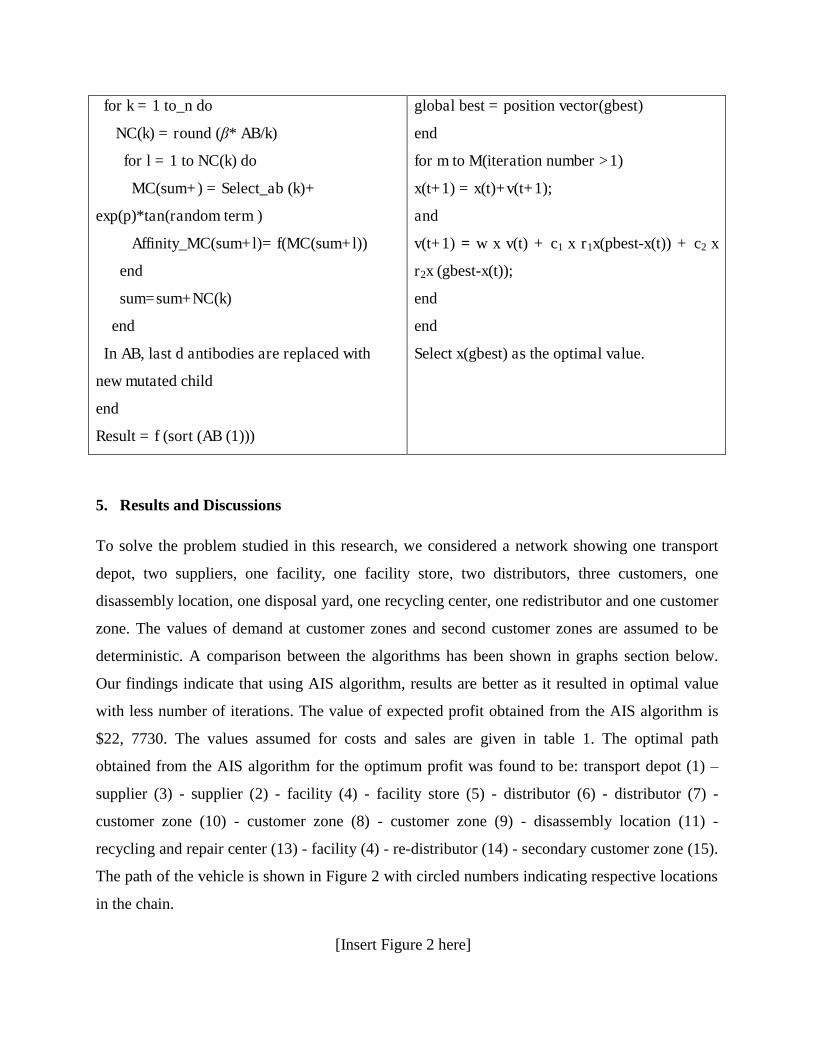
5. Results and Discussions

To solve the problem studied in this research, we considered a network showing one transport

depot, two suppliers, one facility, one facility store, two distributors, three customers, one

disassembly location, one disposal yard, one recycling center, one redistributor and one customer

zone. The values of demand at customer zones and second customer zones are assumed to be

deterministic. A comparison between the algorithms has been shown in graphs section below.

Our findings indicate that using AIS algorithm, results are better as it resulted in optimal value

with less number of iterations. The value of expected profit obtained from the AIS algorithm is

$22, 7730. The values assumed for costs and sales are given in table 1. The optimal path

obtained from the AIS algorithm for the optimum profit was found to be: transport depot (1) –

supplier (3) - supplier (2) - facility (4) - facility store (5) - distributor (6) - distributor (7) -

customer zone (10) - customer zone (8) - customer zone (9) - disassembly location (11) -

recycling and repair center (13) - facility (4) - re-distributor (14) - secondary customer zone (15).

The path of the vehicle is shown in Figure 2 with circled numbers indicating respective locations

in the chain.

[Insert Figure 2 here]

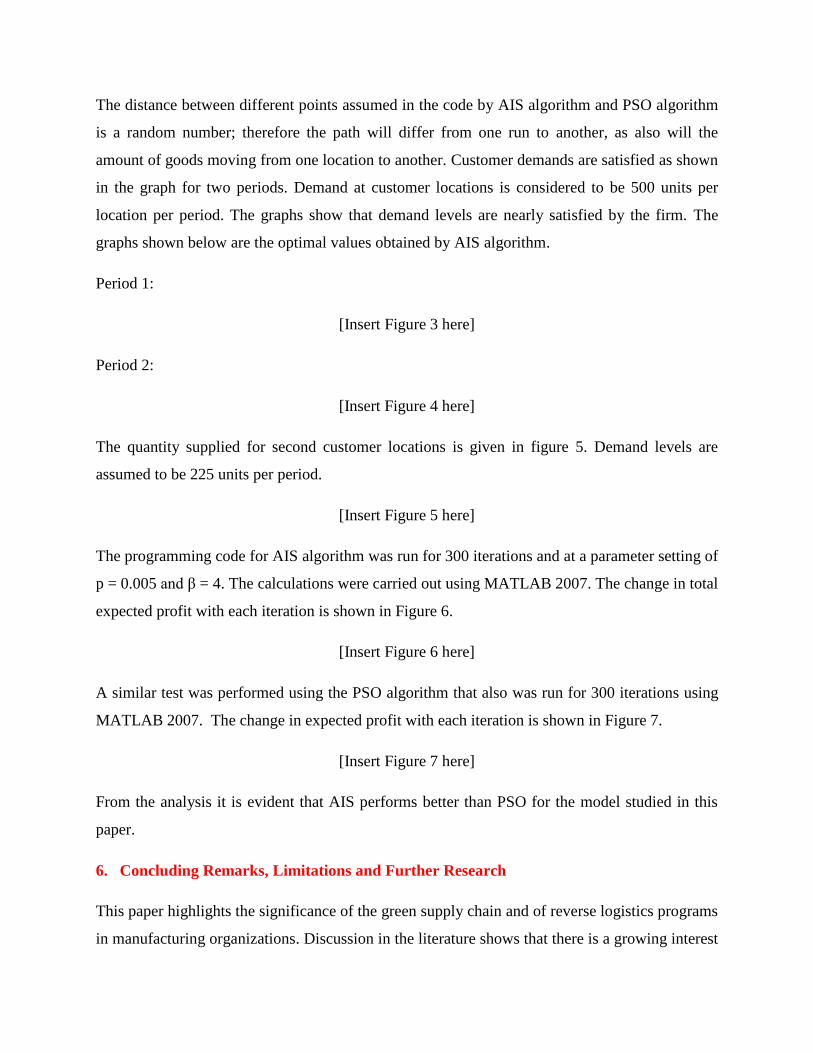
The distance between different points assumed in the code by AIS algorithm and PSO algorithm

is a random number; therefore the path will differ from one run to another, as also will the

amount of goods moving from one location to another. Customer demands are satisfied as shown

in the graph for two periods. Demand at customer locations is considered to be 500 units per

location per period. The graphs show that demand levels are nearly satisfied by the firm. The

graphs shown below are the optimal values obtained by AIS algorithm.

Period 1:

[Insert Figure 3 here]

Period 2:

[Insert Figure 4 here]

The quantity supplied for second customer locations is given in figure 5. Demand levels are

assumed to be 225 units per period.

[Insert Figure 5 here]

The programming code for AIS algorithm was run for 300 iterations and at a parameter setting of

p = 0.005 and く = 4. The calculations were carried out using MATLAB 2007. The change in total

expected profit with each iteration is shown in Figure 6.

[Insert Figure 6 here]

A similar test was performed using the PSO algorithm that also was run for 300 iterations using

MATLAB 2007. The change in expected profit with each iteration is shown in Figure 7.

[Insert Figure 7 here]

From the analysis it is evident that AIS performs better than PSO for the model studied in this

paper.

6. Concluding Remarks, Limitations and Further Research

This paper highlights the significance of the green supply chain and of reverse logistics programs

in manufacturing organizations. Discussion in the literature shows that there is a growing interest

among the research community to address reverse logistics issues. Rising environmental

awareness and changing regulations has forced manufacturing industries to focus on green

sustainable practices. As a result, the manufacturing industry is emphasizing the efficient

handling of their reverse logistics operations while aiming at simultaneously minimizing their

costs and increasing their profitability. This study therefore addresses this issue by particularly

focusing on and proposing a forward and reverse logistics model based on the optimum routing

of vehicles. In particular, this paper puts forward a model of a multi-period, multi-echelon,

vehicle routing, forward-reverse logistics system. The network considered in the model assumes

a fixed number of suppliers, facilities, distributors, customer zones, disassembly locations, re-

distributors and second customer zones. The demand levels at customer zones are assumed to be

deterministic. The proposed model has proved to be useful in obtaining the route of the vehicle,

maximizing the profit and providing information to the firm about the quantities to be produced

at the facility and amount of goods to be obtained from the supplier. This study applies the AIS

and PSO algorithms to determine the optimal route and quantity produced more efficiently. This

paper also shows that for the considered model, AIS works better than the PSO.

Therefore, from a theoretical perspective this paper contributes to the limited literature on

reverse logistics that considers costs, profit as well as vehicle route management. Additionally,

the paper shows the efficacy of the AIS over PSO in resolving the forward reverse logistics

model, thus suggesting that researchers should seek further evidence to see if this applies for

other models. These contributions are beneficial for manufacturing organizations that are

engaged in reverse logistics operations. For example, relevant managers in these organizations

can learn from the proposed model and use it as a reference to optimize the reverse operations of

their organizations. In particular, the proposed model can help managers to have better visibility

of the demand and supply while also efficiently managing the vehicle routing. This can

effectively lead to a maximization of the organization’s profits. Due to the high relevance of

reverse logistics and the growing attention paid to this type of operation, other industries where

this approach has been applied, for example repair service (Amini et al., 2005), post-service (Du

and Evans, 2008) and healthcare (Ritchie et al., 2000), are also likely to benefit from this

research and the proposed model. All these sectors are under constant pressure to operate

competitively and the effective implementation and optimization of reverse logistics operations

provide them with this opportunity.

Like all researches, this paper has a number of limitations. For instance, the values of the

parameters used to test the model in this paper are assumed deterministic values. Therefore,

future research studies should aim at empirically testing the model and algorithm in a realistic

industrial scenario. Working closely with some manufacturing organizations, collecting real data

and testing should be an interesting area for future investigation. This model can be further

extended to a stochastic model by considering mean and variance of demand at different

customer locations. Therefore, the research has adequate scope for further extension. Some

parameters were considered to be fixed to ease the solution method in this research; future work

may involve testing the model by randomly generating the parameters. Vehicle routing can also

be extended by considering capacity constraints for vehicle. Although this study tested the model

using two evolutionary algorithms where AIS emerged as a better alternative, future work may

also involve testing the model using other evolutionary algorithms and comparing the solutions

with hybrid algorithms.

References

Abdulrahman, M. D., Gunasekaran, A., & Subramanian, N. (2014). Critical barriers in

implementing reverse logistics in the Chinese manufacturing sectors. International Journal of

Production Economics, 147 (B), 460-471.

Ageron, B., Gunasekaran, A., Spalanzani, A. (2013). IS/IT as supplier selection criterion for

upstream value chain”, Industrial Management & Data Systems. 113(3), 443 – 460.

Amini, M.M., Retzlaff-Roberts, D., Bienstock, C.C. (2005). Designing a reverse logistics

operation for short cycle time repair services. International Journal of Production Economics,

96(3), 367-380.

Bachlaus, M., Pandey, M. K., Mahajan, C., Shankar, R. and Tiwari, M. K. (2008). Designing an

integrated multi-echelon agile supply chain network: a hybrid taguchi-particle swarm

optimization approach, Journal of Intelligent Manufacturing, 19 (6), 747-761.

Brix-Asala, C., Hahn, R., & Seuring, S. (2016). Reverse logistics and informal valorisation at the

Base of the Pyramid: A case study on sustainability synergies and trade-offs. European

Management Journal (In Press)

Bhattacharya, A., Mohapatra, P., Kumar, V., Dey, P. K., Brady, M., Tiwari, M. K., &

Nudurupati, S. S. (2014). Green supply chain performance measurement using fuzzy ANP-based

balanced scorecard: a collaborative decision-making approach. Production Planning & Control,

25(8), 698-714.

Carvalho, H., Azevedo, S.G., Cruz-Machado, V. (2014). Supply chain management resilience: a

theory building approach. International Journal of Supply Chain and Operations Resilience,

1(1), 3-27.

Chan, F. T. S., Kumar, V. and Tiwari, M. K. (2006). Optimizing the Performance of an

Integrated Process Planning and Scheduling Problem: An AIS-FLC based Approach, 2006 IEEE

Conference on Cybernetics and Intelligent Systems (CIS), Bangkok, 298-305

Chan, H. K., Yin, S. and Chan, F. T. S. (2010). Implementing just-in-time philosophy to reverse

logistics systems: a review, International Journal of Production Research, 48 (21), 6293 – 6313.

Chen, C. X., Chen, Y., & YU, Z. B. (2005). Under the Circular Economy the Development of the

Third Provider Reverse Logistics. Logistics Management, 6, 013.

Choudhary, A. K., Sarkar, S., Settur S., and Tiwari, M. K. (2015). A carbon-footprint

optimization model for integrated forward-reverse logistics, International Journal of Production

Economics, 164, 433–444.

Chiang, T. C., & Lin, H. J. (2013). A simple and effective evolutionary algorithm for

multiobjective flexible job shop scheduling. International Journal of Production Economics,

141(1), 87-98.

De Brito, M. P. and Dekkar, R. (2002). Reverse Logistics – a framework, Econometric Institute

Report, EI (38), Erasmus University Rotterdam, Econometric Institute.

De Castro, L.N. and Von Zuben, F. J. (2001). Learning and Optimization Using the Clonal

Selection Principle, IEEE Trans on Evolutionary Computation, 6 (3), 239 – 251.

De Castro, L. N., and Von Zuben, F. J. (2001). aiNet: An Artificial Immune Network for Data

Analysis, In Data Mining: A Heuristic approach Hussein A. Abbass, Ruhul A. Sarker, and

Charles S. Newton (Eds.) Idea Group Publishing, USA, 1-37.

Dadhich, P., Genovese, A., Kumar, N., Acquaye, A. (2015). Developing sustainable supply

chains in the UK construction industry: A case study. International Journal of Production

Economics, 164, 271-284.

De Castro, L. N. and Timmis, J. (2002). Artificial Immune Systems: A Novel Paradigm to

Pattern Recognition, In Artificial Neural Networks in Pattern Recognition, SOCO-2002,

(University of Paisley, UK), 67-84.

de la Fuente, M. V., Ros, L., & Cardos, M. (2008). Integrating forward and reverse supply

chains: application to a metal-mechanic company. International Journal of Production

Economics, 111(2), 782-792.

De Giovanni, P., Reddy, P.V., Zaccour, G. (2015). Incentive strategies for an optimal recovery

program in a closed-loop supply chain. European Journal of Operational Research, 249(2), 605-

617..

Dethloff, J. (2001).Vehicle routing and reverse logistics: the vehicle routing problem with

simultaneous delivery and pickup, OR Spectrum, 23 (1), 79-96

Diana, R. O. M., de França Filho, M. F., de Souza, S. R., & de Almeida Vitor, J. F. (2015). An

immune-inspired algorithm for an unrelated parallel machines’ scheduling problem with

sequence and machine dependent setup-times for makespan minimization, Neurocomputing, 163,

94-105.

Dowlatshahi, S. (2010). The role of transportation in the design and implementation of reverse

logistics systems, International Journal of Production Research, 48 (14), 4199-4215

Dowlatshahi, S. (2000). Developing a Theory of Reverse Logistics, Interfaces, 30 (3), 143-155.

Du, F., Evans, G.W. (2008). A bi-objective reverse logistics network analysis for post-sale

service, Computers & Operations Research, 35(8), 2617-2634.

El-Sayed, M., Afia, N., and El-Kharbotly, A., (2010). A stochastic model for forward-reverse

logistics network design under risk, Computers & Industrial Engineering, 58 (3), 423-431.

Engin, O. and Doyen, A., (2004). A new approach to solve hybrid flow shop scheduling

problems by artificial immune system, Future Generation Computer Systems, 20 (6), 1083-1095.

Finne, M., Holmström, J. (2013). A manufacturer moving upstream: triadic collaboration for

service delivery. Supply Chain Management: An International Journal, 18(1), 21 – 33.

Fleishman, M., Bloemhof-Ruwaard, J. M., Dekkar, R., van der Laan, E., van nunen, Jo A. E. E.,

and van Wassenhove, L. N. (1997). Quantitative models for reverse logistics: A review,

European Journal of Operational Research, 103 (1), 1-17.

García-Rodríguez, F. J., Castilla-Gutiérrez, C., & Bustos-Flores, C. (2013). Implementation of

reverse logistics as a sustainable tool for raw material purchasing in developing countries: The

case of Venezuela. International Journal of Production Economics, 141(2), 582-592.

Genovese, A., Acquaye, A.A., Figueroa, A., Koh, S.C.L. (2015). Sustainable supply chain

management and the transition towards a circular economy: Evidence and some applications.

Omega, DOI: 10.1016/j.omega.2015.05.015 (in press).

Green, K.W. Jr, Zelbst, P.J., Meacham, J. and Bhadauria, V.S. (2012). Green supply chain

management practices: impact on performance. Supply Chain Management: An International

Journal, 17(3), 290-305.

Hassini, E., Surti, C., Searcy, C. (2012). A literature review and a case study of sustainable

supply chains with a focus on metrics. International Journal of Production Economics, 140(1),

pp. 69-82.

Huang, Y.C., Wu, J.Y.C., Rahman, S. (2012). The task environment, resource commitment and

reverse logistics performance: evidence from the Taiwanese high-tech sector. Production,

Planning & Control, 23 (10-11), 851-863.

Jabbour, C.J.C., Neto, A.S., Gobbo Jr., J.A., de Souza Ribeiro, M., Lopes de Sousa Jabbour,

A.B. (2015). Eco-innovations in more sustainable supply chains for a low-carbon economy: A

multiple case study of human critical success factors in Brazilian leading companies.

International Journal of Production Economics. 164, 245-257.

Janeway, C. A. Jr., (1992). The immune System Evolved to Discriminate Infectious Nonself

from Noninfectious Self, Immunol Today, 13 (1), 11-16.

Johnsen, T.E. (2011). Supply network delegation and intervention strategies during supplier

involvement in new product development. International Journal of Operations & Production

Management, 31(6), 686-708.

Kannan, V.R., Tan, K.C. (2004). Supplier alliances: differences in attitudes to supplier and

quality management of adopters and nonǦadopters. Supply Chain Management: An International

Journal, 9(4), 279 – 286.

Kennedy, J. (2010). Particle swarm optimization, In Encyclopedia of Machine Learning,

Springer US, 760-766.

Kim, J. S., and Lee, D. H. (2015). A case study on collection network design, capacity planning

and vehicle routing in reverse logistics, International Journal of Sustainable Engineering, 8(1),

66-76.

Kheljani, J. G., Ghodsypour, S. H., & O’Brien, C. (2009). Optimizing whole supply chain

benefit versus buyer's benefit through supplier selection. International Journal of Production

Economics, 121(2), 482-493.

Ko, H. J. and Evans, G. W. (2007). A genetic algorithm-based heuristic for the dynamic

integrated forward/reverse logistics network for 3PLs, Computers & Operations Research, 34

(2), 346-366.

Kroon, L. and Vrijens, G. (1994). Returnable containers: an example of reverse logistics,

International Journal of Physical Distribution & Logistics Management, 25 (2), 56-68.

Kumar, V., Holt, D., Ghobadian, A., & Garza-Reyes, J. A. (2015). Developing green supply

chain management taxonomy-based decision support system, International Journal of

Production Research, 53 (1), 6372-6389.

Kumar, V, Prakash, Tiwari, M. K., Chan, F. T.S. (2006). Stochastic make-to-stock inventory

deployment problem: an endosymbiotic psychoclonal algorithm based approach, International

Journal of Production Research, 44 (11), 2245-2263.

Kumar, V., Mishra, N., Chan, F. T., and Verma, A. (2011). Managing warehousing in an agile

supply chain environment: an F-AIS algorithm based approach, International Journal of

Production Research, 49(21), 6407-6426.

Lee, P.K.C., Yeung, A.C.L., Cheng, T.C.E., (2009). Supplier alliances and environmental

uncertainty: An empirical study. International Journal of Production Economics, 120(1), 190-

204.

Li, S., Rao, S.S., Ragu-Nathan, T.S., Ragu-Nathan, B. (2005). Development and validation of a

measurement instrument for studying supply chain management practices. Journal of Operations

Management, 23(6), 618-641.

Li, S., Ragu-Nathan, B., Ragu-Nathan, T.S., Rao, S.S. (2006). The impact of supply chain

management practices on competitive advantage and organizational performance. Omega, 34(2),

107-124.

Li, T., Zhang, H. (2015). Information sharing in a supply chain with a make-to-stock

manufacturer. Omega, 50, 115-125.

Mishra, N., Kumar, V., and Chan, F. T. (2012). A multi-agent architecture for reverse logistics in

a green supply chain, International Journal of Production Research, 50(9), 2396-2406.

Meng, Liu. (2013). Study on Establishing Reverse Logistics System in Environment of Circular

Economy. Logistics Technology, 5, 66.

Mohanty, R.P., Prakash, A. (2014). Green supply chain management practices in India: an

empirical study. Production Planning & Control. 25 (16), 1322-1337.

Moslehi, G., & Mahnam, M. (2011). A Pareto approach to multi-objective flexible job-shop

scheduling problem using particle swarm optimization and local search, International Journal of

Production Economics, 129(1), 14-22.

Narasimhan, R., Schoenherr, T. (2012). The effects of integrated supply management practices

and environmental management practices on relative competitive quality advantage.

International Journal of Production Research, 50(4), 1185-1201.

Oosterhuis, M., van der Vaart, T., Molleman, E. (2012). The value of upstream recognition of

goals in supply chains. Supply Chain Management: An International Journal, 17(6), 582 – 595.

Pan, S.Y., Du, M.D., Huang, I.T., Liu, I.H., Chang, E.E., Chiang, P.C. (2015). Strategies on

implementation of waste-to-energy (WTE) supply chain for circular economy system: a review.

Journal of Cleaner Production, 108(Part A), 409-421.

Pettersson, A. I., & Segerstedt, A. (2013). Measuring supply chain cost. International Journal of

Production Economics, 143(2), 357-363.

Pishvaee, M. S., Farahani, R. Z., and Dullaert, W. (2010). A memetic algorithm for bi-objective

integrated forward/reverse logistics network design, Computers & Operations Research, 37(6),

1100-1112.

Pérez-Cáceres, L., & Riff, M. C. (2015). Solving scheduling tournament problems using a new

version of CLONALG, Connection Science, 27(1), 5-21.

Ravi, V., Shankar, R. and Tiwari, M. K. (2008). Selection of a reverse logistics project for end-

of-life computers: ANP and goal programming approach, International Journal of Production

Research, 46 (17), 4849 – 4870.

Reuter, C., Foerst, K., Hartmann, E., Blome, C. (2010). Sustainable global supplier management:

the role of dynamic capabilities in achieving competitive advantage. Journal of Supply Chain

Management, 46(2), 45-63.

Ritchie, L., Burnes, B., Whittle, P., Hey, R. (2000). The benefits of reverse logistics: the case of

the Manchester Royal Infirmary Pharmacy. Supply Chain Management: An International

Journal, 5(5), 226 - 234

Rogers, D. S. and Tibben-Lembke, R.S. (1999).Going Backwards: Reverse Logistics Trends and

Practices, Pittsburgh. PA: Reverse Logistics Executive Council: USA

Sarkis, J. (2003). A strategic decision framework for green supply chain management. Journal of

Cleaner Production. 11 (4), 397-409.

Sarkis, J., Helms, M. M., & Hervani, A. A. (2010). Reverse logistics and social sustainability.

Corporate Social Responsibility and Environmental Management, 17(6), 337-354.

Shukla, N., Choudhary, A. K., Prakash, P., Fernandes, K., and Tiwari, M.K., (2013). Algorithm

Portfolio for Vehicle Routing Problem with Stochastic Demands and Mobility Allowance.

International Journal of Production Economics, 141(1), 146-166.

Soysal, M., Bloemhof-Ruwaard, J. M., Haijema, R., & van der Vorst, J. G. (2015). Modeling an

Inventory Routing Problem for perishable products with environmental considerations and

demand uncertainty. International Journal of Production Economics, 164, 118-133.

Srivastava (2007), S.K. (2007), Green supply-chain management: A state-of-the-art literature

review. International Journal of Management Reviews, 9(1), 53-80.

Tan, K.C., Lyman, S.B., Wisner, J.D. (2002). Supply chain management: a strategic perspective.

International Journal of Operations & Production Management, 22(6), 614–31.

Teodorović, D., Lučić, P., Marković, G., & Dell'Orco, M. (2006). Bee colony optimization:

principles and applications. In Neural Network Applications in Electrical Engineering, NEUREL

2006, 8th Seminar on IEEE, 151-156

Teunter, R. H. (2001). A reverse logistics valuation method for inventory control, International

Journal of Production Research, 39 (9), 2023 – 2035

Tiwari, A., & Chang, P. C. (2015). A block recombination approach to solve green vehicle

routing problem, International Journal of Production Economics, 164, 379-387.

Tsai, W. H. and Hung, S. J. (2009). Treatment and recycling system optimization with activity-

based costing in WEEE reverse logistics management: an environmental supply chain

perspective, International Journal of Production Research, 47 (19), 5391-5420.

Ubeda, S., Arcelus, F.J., Faulin, J., (2011). Green logistics at Eroski. International Journal of

Production Economics. 131 (1). 44-51.

Vishwa, V. K., Chan, F. T., Mishra, N., & Kumar, V. (2010). Environmental integrated closed

loop logistics model: an artificial bee colony approach. In Supply Chain Management and

Information Systems (SCMIS), 2010 8th International Conference on IEEE, 1-7.

Viswanadham, N., Samvedi, A. (2013). Supplier selection based on supply chain ecosystem,

performance and risk criteria. International Journal of Production Research, 51(21), 6484-6498.

Wang, X., Chan, H. K., Yee, R. W., & Diaz-Rainey, I. (2012). A two-stage fuzzy-AHP model

for risk assessment of implementing green initiatives in the fashion supply chain. International

Journal of Production Economics, 135(2), 595-606.

Weeks, K., Gao, H., Alidaeec, B., and Rana, D. S. (2010). An empirical study of impacts of

production mix, product route efficiencies on operations performance and profitability: a reverse

logistics approach, International Journal of Production Research, 48 (4), 1087–1104.

White, J. A., and Garrett, S. M. (2003). Improved pattern recognition with artificial clonal

selection? In Artificial Immune Systems (pp. 181-193), Springer Berlin Heidelberg.

Ying, J., Li -jun, Z. (2012). Study on Green Supply Chain Management Based on Circular

Economy. Physics Procedia, 25, 1682–1688.

Zhao, X., Baofeng, H., Flynn, B.B., Yeung, J.H.Y. (2008). The impact of power and relationship

commitment on the integration between manufacturers and customers in a supply chain. Journal

of Operations Management, 26(3), 368-388.

Zheng Y. and Zhang G. (2008). A Genetic Algorithm for Vehicle Routing Problem with forward

and reverse logistics, 4th International Conference on Wireless Communications, Networking

and Mobile Computing, WiCOM '08, 1 – 4.

Zhu, Q., Sarkis, J., Lai, K. (2008). Confirmation of a measurement model for green supply chain

management practices implementation. International Journal of Production Economics. 111 (2),

261-273.

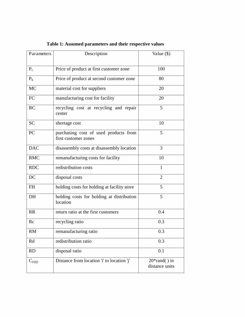
Table 1: Assumed parameters and their respective values

Parameters Description Value ($)

Pc Price of product at first customer zone 100

Pk Price of product at second customer zone 80

MC material cost for suppliers 20

FC manufacturing cost for facility 20

RC recycling cost at recycling and repair center

5

SC shortage cost 10

PC purchasing cost of used products from first customer zones

5

DAC disassembly costs at disassembly location 3

RMC remanufacturing costs for facility 10

RDC redistribution costs 1

DC disposal costs 2

FH holding costs for holding at facility store 5

DH holding costs for holding at distribution location

5

RR return ratio at the first customers 0.4

Rc recycling ratio 0.3

RM remanufacturing ratio 0.3

Rd redistribution ratio 0.3

RD disposal ratio 0.1

C(i)(j) Distance from location 'i' to location 'j' 20*rand( ) in distance units