resistor networks and optimal grids for electrical ... · resistor networks and optimal grids for...

Resistor Networks and Optimal Grids for ElectricalImpedance Tomography with Partial Boundary

Measurements

Alexander Mamonov1,Liliana Borcea2, Vladimir Druskin3,

Fernando Guevara Vasquez4

1Institute for Computational Engineering and Sciences, University of Texas at Austin,2Rice University, 3Schlumberger-Doll Research, 4University of Utah

June 20, 2011

Support: Schlumberger R62860, NSF DMS-0604008, DMS-0934594.

A.V. Mamonov (UT Austin, ICES) 1 / 37

EIT with resistor networks and optimal grids

Electrical Impedance Tomography

1 EIT with resistor networks and optimal grids

2 Conformal and quasi-conformal mappings

3 Pyramidal networks and sensitivity grids

4 Two-sided problem and networks

5 Numerical results

6 Conclusions



Electrical Impedance Tomography: Physical problem

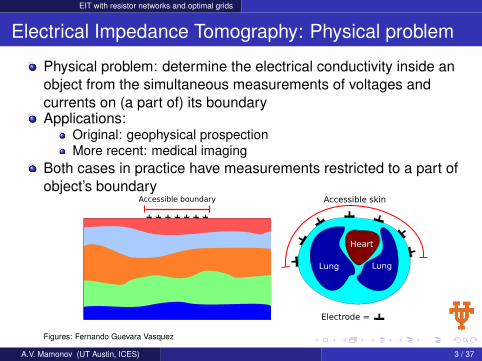
Physical problem: determine the electrical conductivity inside anobject from the simultaneous measurements of voltages andcurrents on (a part of) its boundaryApplications:

Original: geophysical prospectionMore recent: medical imaging

Both cases in practice have measurements restricted to a part ofobject’s boundary

Accessible boundary

Electrode =

Lung

Heart

Lung

Accessible skin

Figures: Fernando Guevara Vasquez



Partial data EIT: mathematical formulation

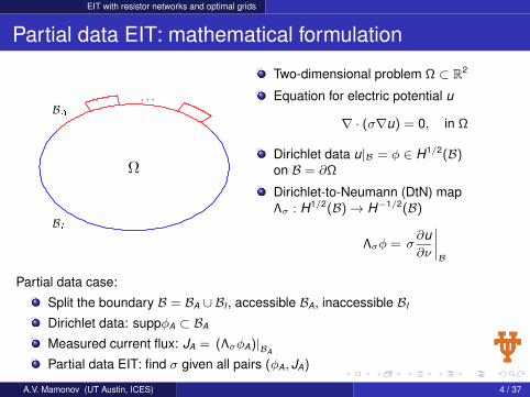
Two-dimensional problem Ω ⊂ R2

Equation for electric potential u

∇ · (σ∇u) = 0, in Ω

Dirichlet data u|B = φ ∈ H1/2(B)on B = ∂Ω

Dirichlet-to-Neumann (DtN) mapΛσ : H1/2(B)→ H−1/2(B)

Λσφ = σ∂u∂ν

∣∣∣∣B

Partial data case:

Split the boundary B = BA ∪ BI , accessible BA, inaccessible BI

Dirichlet data: suppφA ⊂ BA

Measured current flux: JA = (ΛσφA)|BA

Partial data EIT: find σ given all pairs (φA, JA)



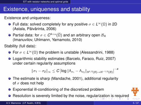
Existence, uniqueness and stabilityExistence and uniqueness:

Full data: solved completely for any positive σ ∈ L∞(Ω) in 2D(Astala, Päivärinta, 2006)

Partial data: for σ ∈ C4+α(Ω) and an arbitrary open BA(Imanuvilov, Uhlmann, Yamamoto, 2010)

Stability (full data):

For σ ∈ L∞(Ω) the problem is unstable (Alessandrini, 1988)

Logarithmic stability estimates (Barcelo, Faraco, Ruiz, 2007)under certain regularity assumptions

‖σ1 − σ2‖∞ ≤ C∣∣log ‖Λσ1 − Λσ2‖H1/2(B)→H−1/2(B)

∣∣−a

The estimate is sharp (Mandache, 2001), additional regularityof σ does not help

Exponential ill-conditioning of the discretized problem

Resolution is severely limited by the noise, regularization is required



Numerical methods for EIT

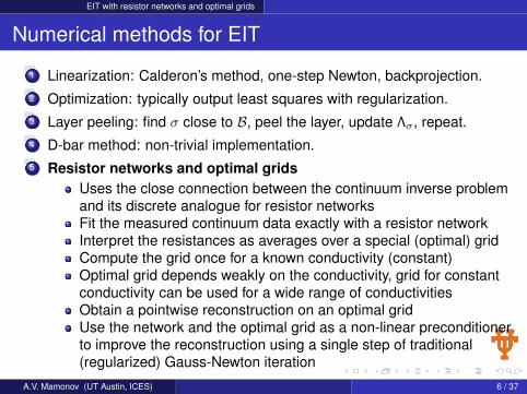
1 Linearization: Calderon’s method, one-step Newton, backprojection.2 Optimization: typically output least squares with regularization.3 Layer peeling: find σ close to B, peel the layer, update Λσ, repeat.4 D-bar method: non-trivial implementation.5 Resistor networks and optimal grids

Uses the close connection between the continuum inverse problemand its discrete analogue for resistor networksFit the measured continuum data exactly with a resistor networkInterpret the resistances as averages over a special (optimal) gridCompute the grid once for a known conductivity (constant)Optimal grid depends weakly on the conductivity, grid for constantconductivity can be used for a wide range of conductivitiesObtain a pointwise reconstruction on an optimal gridUse the network and the optimal grid as a non-linear preconditionerto improve the reconstruction using a single step of traditional(regularized) Gauss-Newton iteration



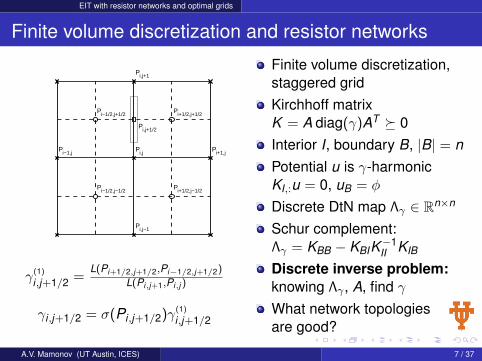
Finite volume discretization and resistor networks

Pi,j

Pi,j+1

Pi,j−1

Pi+1,jPi−1,j

Pi+1/2,j+1/2

Pi+1/2,j−1/2

Pi−1/2,j+1/2

Pi−1/2,j−1/2

Pi,j+1/2

γ(1)

i,j+1/2 =L(Pi+1/2,j+1/2,Pi−1/2,j+1/2)

L(Pi,j+1,Pi,j )

γi,j+1/2 = σ(Pi,j+1/2)γ(1)

i,j+1/2

Finite volume discretization,staggered gridKirchhoff matrixK = A diag(γ)AT 0Interior I, boundary B, |B| = nPotential u is γ-harmonicKI,:u = 0, uB = φ

Discrete DtN map Λγ ∈ Rn×n

Schur complement:Λγ = KBB − KBIK−1

II KIB

Discrete inverse problem:knowing Λγ , A, find γWhat network topologiesare good?



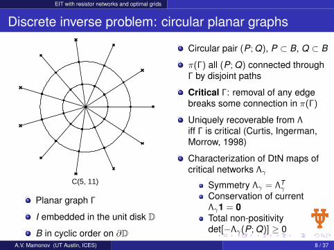
Discrete inverse problem: circular planar graphs

C(5, 11)

Planar graph Γ

I embedded in the unit disk D

B in cyclic order on ∂D

Circular pair (P; Q), P ⊂ B, Q ⊂ B

π(Γ) all (P; Q) connected throughΓ by disjoint paths

Critical Γ: removal of any edgebreaks some connection in π(Γ)

Uniquely recoverable from Λiff Γ is critical (Curtis, Ingerman,Morrow, 1998)

Characterization of DtN maps ofcritical networks Λγ

Symmetry Λγ = ΛTγ

Conservation of currentΛγ1 = 0Total non-positivitydet[−Λγ(P; Q)] ≥ 0



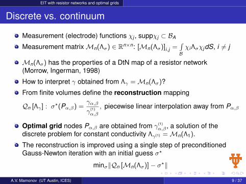
Discrete vs. continuum

Measurement (electrode) functions χj , suppχj ⊂ BA

Measurement matrixMn(Λσ) ∈ Rn×n: [Mn(Λσ)]i,j =∫Bχi ΛσχjdS, i 6= j

Mn(Λσ) has the properties of a DtN map of a resistor network(Morrow, Ingerman, 1998)

How to interpret γ obtained from Λγ =Mn(Λσ)?

From finite volumes define the reconstruction mapping

Qn [Λγ ] : σ?(Pα,β) =γα,β

γ(1)

α,β

, piecewise linear interpolation away from Pα,β

Optimal grid nodes Pα,β are obtained from γ(1)

α,β , a solution of thediscrete problem for constant conductivity Λγ(1) =Mn(Λ1).

The reconstruction is improved using a single step of preconditionedGauss-Newton iteration with an initial guess σ?

minσ‖Qn [Mn(Λσ)]− σ?‖



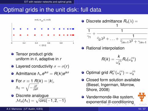
Optimal grids in the unit disk: full data

0 0.2 0.4 0.6 0.8 1r ∈ [0,1]

m=5, m1/2

=1, n=25

Tensor product gridsuniform in θ, adaptive in r

Layered conductivity σ = σ(r)

Admittance Λσeikθ = R(k)eikθ

For σ ≡ 1 R(k) = |k |,Λ1 =

√− ∂2

∂θ2

Discrete analogueMn(Λ1) =

√circ(−1,2,−1)

Discrete admittance Rn(λ) =1

1γ1

+1

γ2λ2 + . . .+1

γm+1λ2 + γm+1

Rational interpolation

R(k) =kω(n)

kRn(ω(n)

k )

Optimal grid R(1)

n (ω(n)

k ) = ω(n)

k

Closed form solution available(Biesel, Ingerman, Morrow,Shore, 2008)

Vandermonde-like system,exponential ill-conditioning


Conformal and quasi-conformal mappings

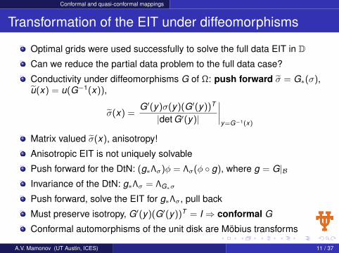
Transformation of the EIT under diffeomorphisms

Optimal grids were used successfully to solve the full data EIT in DCan we reduce the partial data problem to the full data case?

Conductivity under diffeomorphisms G of Ω: push forward σ = G∗(σ),u(x) = u(G−1(x)),

σ(x) =G′(y)σ(y)(G′(y))T

|det G′(y)|

∣∣∣∣y=G−1(x)

Matrix valued σ(x), anisotropy!

Anisotropic EIT is not uniquely solvable

Push forward for the DtN: (g∗Λσ)φ = Λσ(φ g), where g = G|BInvariance of the DtN: g∗Λσ = ΛG∗σ

Push forward, solve the EIT for g∗Λσ, pull back

Must preserve isotropy, G′(y)(G′(y))T = I ⇒ conformal G

Conformal automorphisms of the unit disk are Möbius transforms



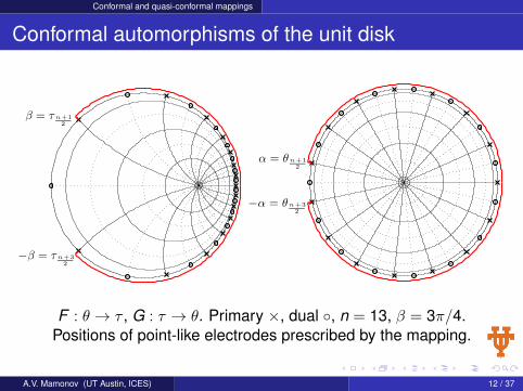
Conformal automorphisms of the unit disk

β = τ n+12

−β = τ n+32

α = θn+12

−α = θn+32

F : θ → τ , G : τ → θ. Primary ×, dual , n = 13, β = 3π/4.Positions of point-like electrodes prescribed by the mapping.



Conformal mapping grids: limiting behavior

β = ξ−1

−β = ξ1

π = ξ0

ξ−2

ξ2

ξ−3

ξ3

ξ−4

ξ4

ξ−5

ξ5

ξ−6

ξ6

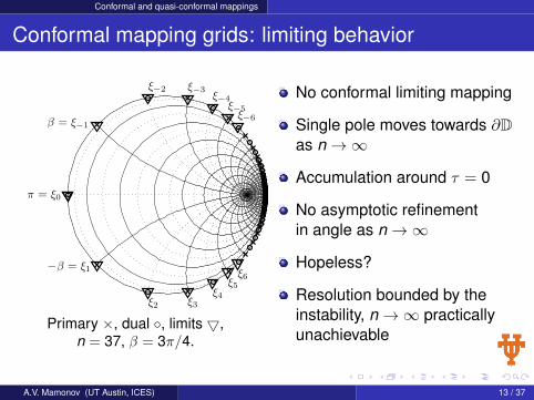
Primary ×, dual , limits 5,n = 37, β = 3π/4.

No conformal limiting mapping

Single pole moves towards ∂Das n→∞

Accumulation around τ = 0

No asymptotic refinementin angle as n→∞

Hopeless?

Resolution bounded by theinstability, n→∞ practicallyunachievable



Quasi-conformal mappings

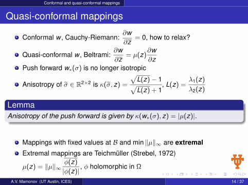
Conformal w , Cauchy-Riemann:∂w∂z

= 0, how to relax?

Quasi-conformal w , Beltrami:∂w∂z

= µ(z)∂w∂z

Push forward w∗(σ) is no longer isotropic

Anisotropy of σ ∈ R2×2 is κ(σ, z) =

√L(z)− 1√L(z) + 1

, L(z) =λ1(z)

λ2(z)

LemmaAnisotropy of the push forward is given by κ(w∗(σ), z) = |µ(z)|.

Mappings with fixed values at B and min ‖µ‖∞ are extremal

Extremal mappings are Teichmüller (Strebel, 1972)

µ(z) = ‖µ‖∞φ(z)

|φ(z)| , φ holomorphic in Ω



Computing the extremal quasi-conformal mappings

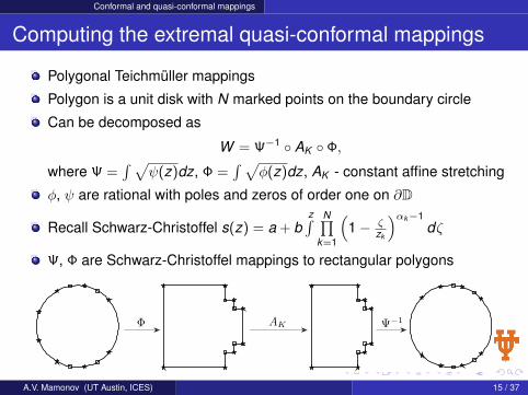
Polygonal Teichmüller mappings

Polygon is a unit disk with N marked points on the boundary circle

Can be decomposed as

W = Ψ−1 AK Φ,

where Ψ =∫ √

ψ(z)dz, Φ =∫ √

φ(z)dz, AK - constant affine stretching

φ, ψ are rational with poles and zeros of order one on ∂D

Recall Schwarz-Christoffel s(z) = a + bz∫ N∏

k=1

(1− ζ

zk

)αk−1dζ

Ψ, Φ are Schwarz-Christoffel mappings to rectangular polygons

Φ AK Ψ−1



Polygonal Teichmüller mapping: the grids

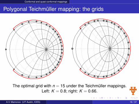
The optimal grid with n = 15 under the Teichmüller mappings.Left: K = 0.8; right: K = 0.66.


Pyramidal networks and sensitivity grids

EIT with pyramidal networks: motivation

v1

v2

v3 v4

v5

v6

v1

v2

v3

v4

v5

v6

v7

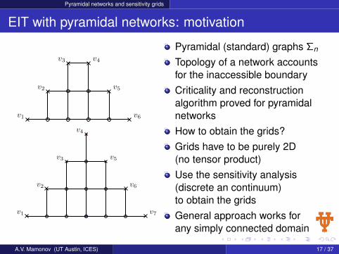
Pyramidal (standard) graphs Σn

Topology of a network accountsfor the inaccessible boundaryCriticality and reconstructionalgorithm proved for pyramidalnetworksHow to obtain the grids?Grids have to be purely 2D(no tensor product)Use the sensitivity analysis(discrete an continuum)to obtain the gridsGeneral approach works forany simply connected domain



Special solutions and recovery

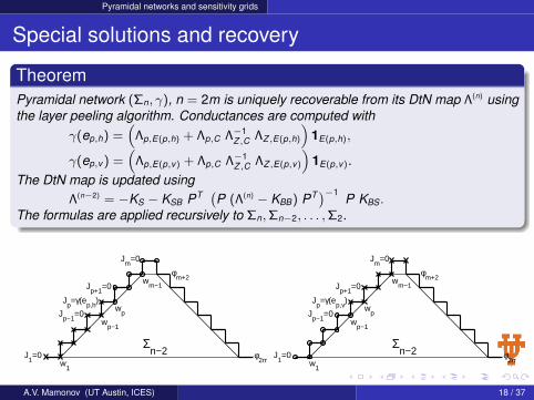
TheoremPyramidal network (Σn, γ), n = 2m is uniquely recoverable from its DtN map Λ(n) usingthe layer peeling algorithm. Conductances are computed with

γ(ep,h) =(

Λp,E(p,h) + Λp,C Λ−1Z ,C ΛZ ,E(p,h)

)1E(p,h),

γ(ep,v ) =(

Λp,E(p,v) + Λp,C Λ−1Z ,C ΛZ ,E(p,v)

)1E(p,v).

The DtN map is updated usingΛ(n−2) = −KS − KSB PT (

P (Λ(n) − KBB) PT )−1P KBS .

The formulas are applied recursively to Σn,Σn−2, . . . ,Σ2.

Σn−2J

1=0

Jp−1

=0

Jp=γ(e

p,h)

Jp+1

=0

Jm

=0

w1

wp−1

wp

wm−1

φm+2

φ2m

Σn−2J

1=0

Jp−1

=0

Jp=γ(e

p,v)

Jp+1

=0

Jm

=0

w1

wp−1

wp

wm−1

φm+2

φ2m



Sensitivity grids: motivation



Sensitivity grids

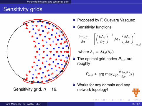
Sensitivity grid, n = 16.

Proposed by F. Guevara Vasquez

Sensitivity functions

δγα,βδσ

=

[(∂Λγ∂γ

)−1

Mn

(δΛσδσ

)]α,β

where Λγ =Mn(Λσ)

The optimal grid nodes Pα,β areroughly

Pα,β ≈ arg maxx∈Ω

δγα,βδσ

(x)

Works for any domain and anynetwork topology!


Two-sided problem and networks

Two sided problem and networks

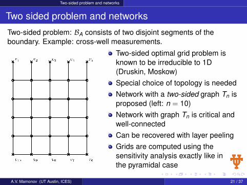
Two-sided problem: BA consists of two disjoint segments of theboundary. Example: cross-well measurements.

Two-sided optimal grid problem isknown to be irreducible to 1D(Druskin, Moskow)Special choice of topology is neededNetwork with a two-sided graph Tn isproposed (left: n = 10)Network with graph Tn is critical andwell-connectedCan be recovered with layer peelingGrids are computed using thesensitivity analysis exactly like inthe pyramidal case


Two-sided problem and networks

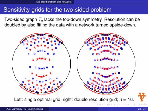
Sensitivity grids for the two-sided problem

Two-sided graph Tn lacks the top-down symmetry. Resolution can bedoubled by also fitting the data with a network turned upside-down.

Left: single optimal grid; right: double resolution grid; n = 16.


Numerical results

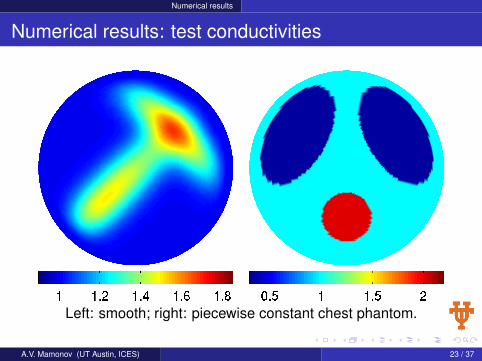
Numerical results: test conductivities

Left: smooth; right: piecewise constant chest phantom.


Numerical results

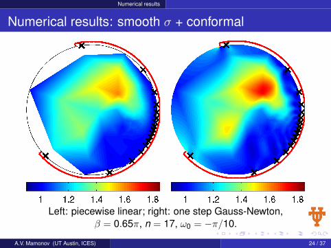
Numerical results: smooth σ + conformal

Left: piecewise linear; right: one step Gauss-Newton,β = 0.65π, n = 17, ω0 = −π/10.


Numerical results

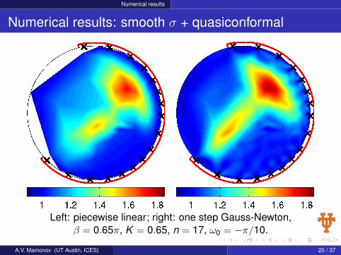
Numerical results: smooth σ + quasiconformal

Left: piecewise linear; right: one step Gauss-Newton,β = 0.65π, K = 0.65, n = 17, ω0 = −π/10.


Numerical results

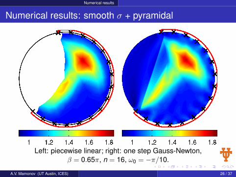
Numerical results: smooth σ + pyramidal

Left: piecewise linear; right: one step Gauss-Newton,β = 0.65π, n = 16, ω0 = −π/10.


Numerical results

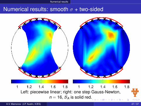
Numerical results: smooth σ + two-sided

Left: piecewise linear; right: one step Gauss-Newton,n = 16, BA is solid red.


Numerical results

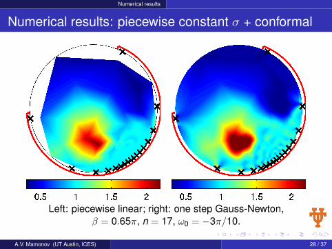
Numerical results: piecewise constant σ + conformal

Left: piecewise linear; right: one step Gauss-Newton,β = 0.65π, n = 17, ω0 = −3π/10.


Numerical results

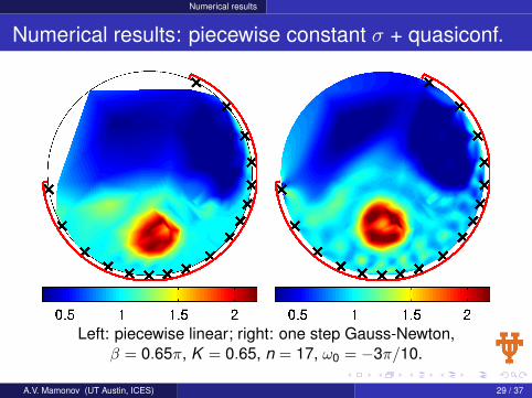
Numerical results: piecewise constant σ + quasiconf.

Left: piecewise linear; right: one step Gauss-Newton,β = 0.65π, K = 0.65, n = 17, ω0 = −3π/10.


Numerical results

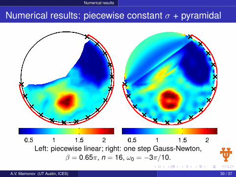
Numerical results: piecewise constant σ + pyramidal

Left: piecewise linear; right: one step Gauss-Newton,β = 0.65π, n = 16, ω0 = −3π/10.


Numerical results

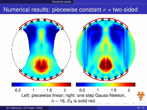
Numerical results: piecewise constant σ + two-sided

Left: piecewise linear; right: one step Gauss-Newton,n = 16, BA is solid red.


Numerical results

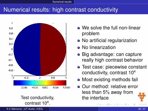
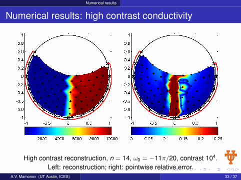
Numerical results: high contrast conductivity

Test conductivity,contrast 104.

We solve the full non-linearproblemNo artificial regularizationNo linearizationBig advantage: can capturereally high contrast behaviorTest case: piecewise constantconductivity, contrast 104

Most existing methods failOur method: relative errorless than 5% away fromthe interface


Numerical results

Numerical results: high contrast conductivity

High contrast reconstruction, n = 14, ω0 = −11π/20, contrast 104.Left: reconstruction; right: pointwise relative error.


Numerical results

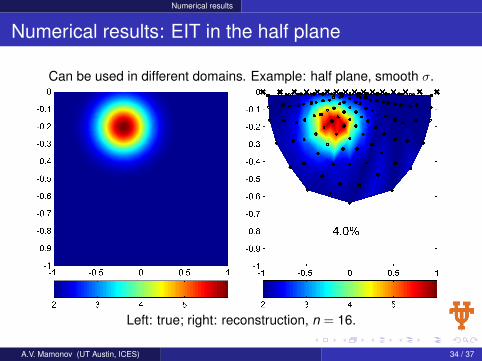
Numerical results: EIT in the half plane

Can be used in different domains. Example: half plane, smooth σ.

Left: true; right: reconstruction, n = 16.


Numerical results

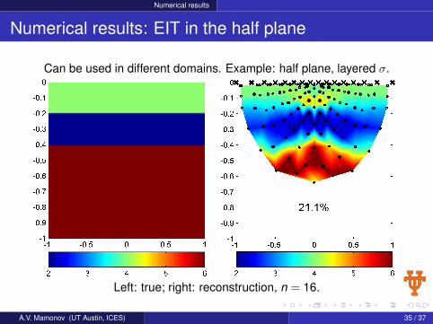
Numerical results: EIT in the half plane

Can be used in different domains. Example: half plane, layered σ.

Left: true; right: reconstruction, n = 16.


Conclusions

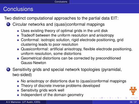
Conclusions

Two distinct computational approaches to the partial data EIT:1 Circular networks and (quasi)conformal mappings

Uses existing theory of optimal grids in the unit diskTradeoff between the uniform resolution and anisotropyConformal: isotropic solution, rigid electrode positioning, gridclustering leads to poor resolutionQuasiconformal: artificial anisotropy, flexible electrode positioning,uniform resolution, some distortionsGeometrical distortions can be corrected by preconditionedGauss-Newton

2 Sensitivity grids and special network topologies (pyramidal,two-sided)

No anisotropy or distortions due to (quasi)conformal mappingsTheory of discrete inverse problems developedSensitivity grids work wellIndependent of the domain geometry


Conclusions

References

Uncertainty quantification for electrical impedance tomographywith resistor networks, L. Borcea, F. Guevara Vasquez andA.V. Mamonov. Preprint: arXiv:1105.1183 [math-ph]Pyramidal resistor networks for electrical impedance tomographywith partial boundary measurements, L. Borcea, V. Druskin,A.V. Mamonov and F. Guevara Vasquez. Inverse Problems26(10):105009, 2010.Circular resistor networks for electrical impedance tomographywith partial boundary measurements, L. Borcea, V. Druskin andA.V. Mamonov. Inverse Problems 26(4):045010, 2010.Electrical impedance tomography with resistor networks,L. Borcea, V. Druskin and F. Guevara Vasquez. Inverse Problems24(3):035013, 2008.


resistor networks and optimal grids for electrical ... · resistor networks and optimal grids for...

Documents