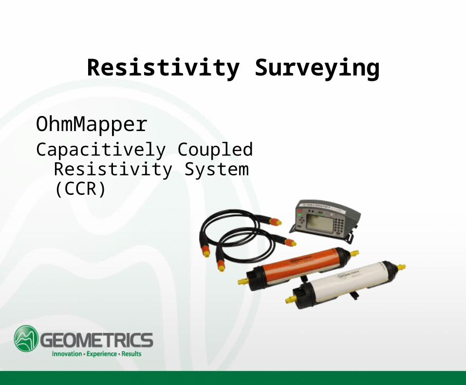
Resistivity Surveying

OhmMapper Capacitively Coupled Resistivity

System (CCR)

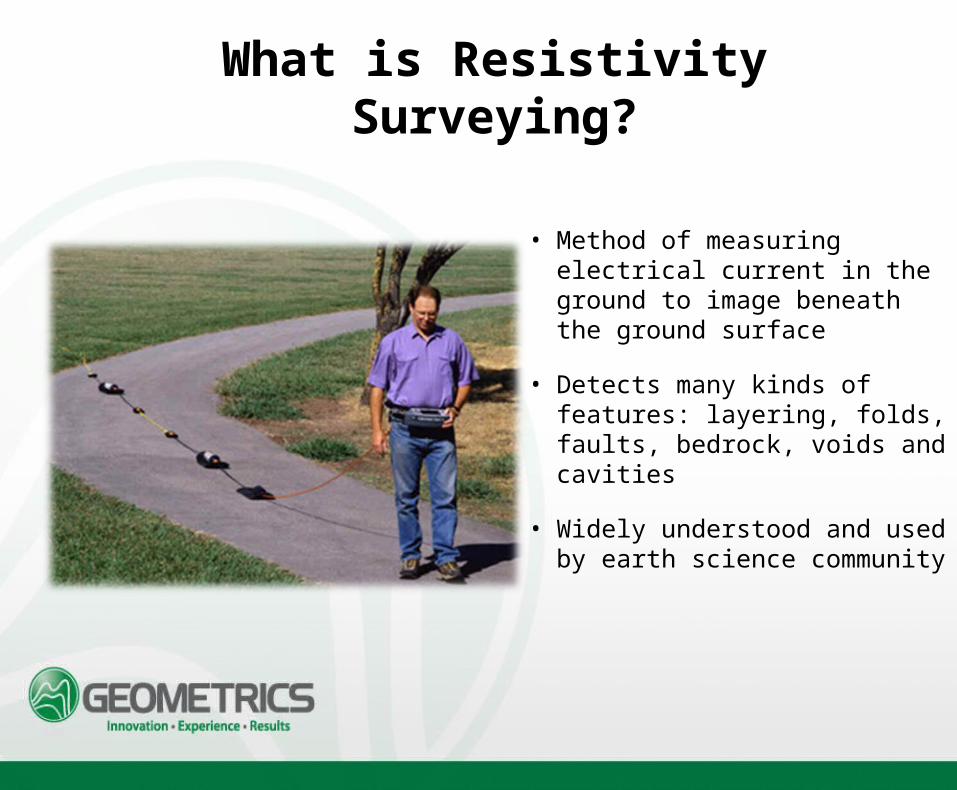
What is Resistivity Surveying?

• Method of measuring electrical current in the ground to image beneath the ground surface

• Detects many kinds of features: layering, folds, faults, bedrock, voids and cavities

• Widely understood and used by earth science community

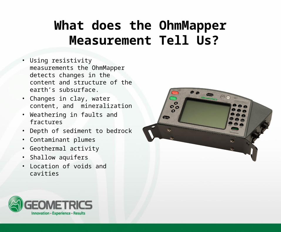
What does the OhmMapper Measurement Tell Us?

• Using resistivity measurements the OhmMapper detects changes in the content and structure of the earth’s subsurface.

• Changes in clay, water content, and mineralization

• Weathering in faults and fractures• Depth of sediment to bedrock• Contaminant plumes• Geothermal activity• Shallow aquifers• Location of voids and cavities

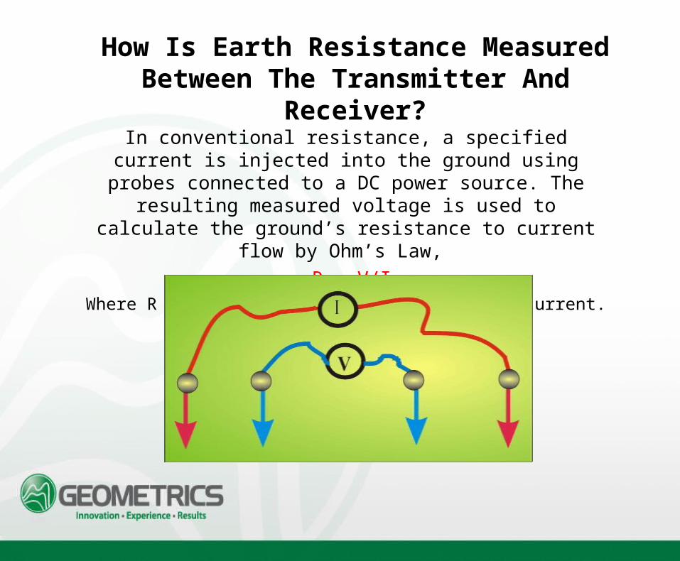
How Is Earth Resistance Measured Between The Transmitter And Receiver?

In conventional resistance, a specified current is injected into the ground using probes connected to a DC power source. The resulting measured voltage is used to calculate the ground’s resistance to current

flow by Ohm’s Law, R = V/I,

Where R = resistance, V = voltage, and I = current.

.

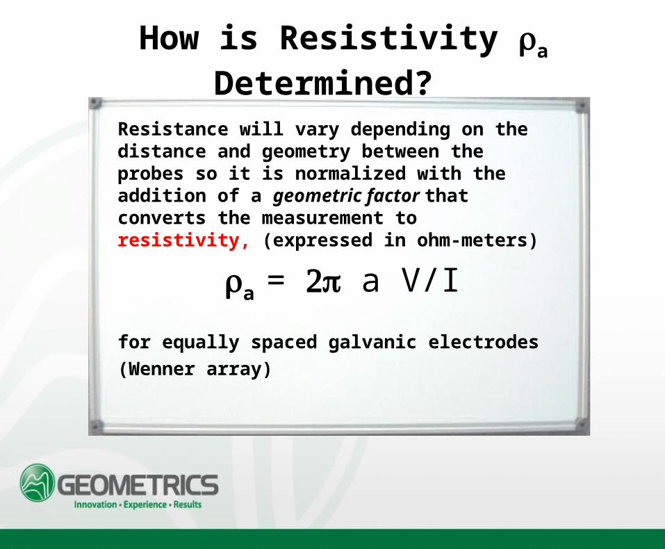
How is Resistivity a Determined?

Resistance will vary depending on the distance and geometry between the probes so it is normalized with the addition of a geometric factor that converts the measurement to resistivity, (expressed in ohm-meters)

a = a V/I

for equally spaced galvanic electrodes (Wenner array)

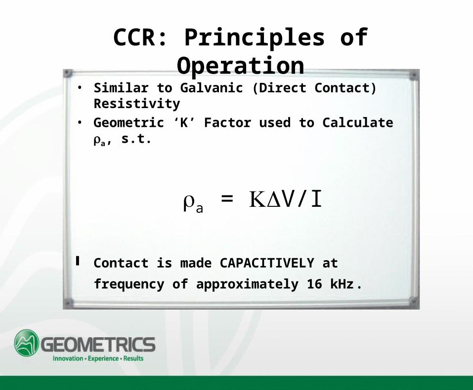
CCR: Principles of Operation• Similar to Galvanic (Direct Contact)

Resistivity• Geometric ‘K’ Factor used to Calculate

a, s.t.

a = V/I

Contact is made CAPACITIVELY at

frequency of approximately 16 kHz.

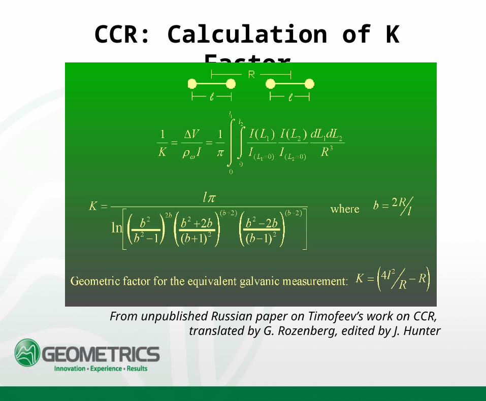
CCR: Calculation of K Factor

From unpublished Russian paper on Timofeev’s work on CCR, translated by G. Rozenberg, edited by J. Hunter

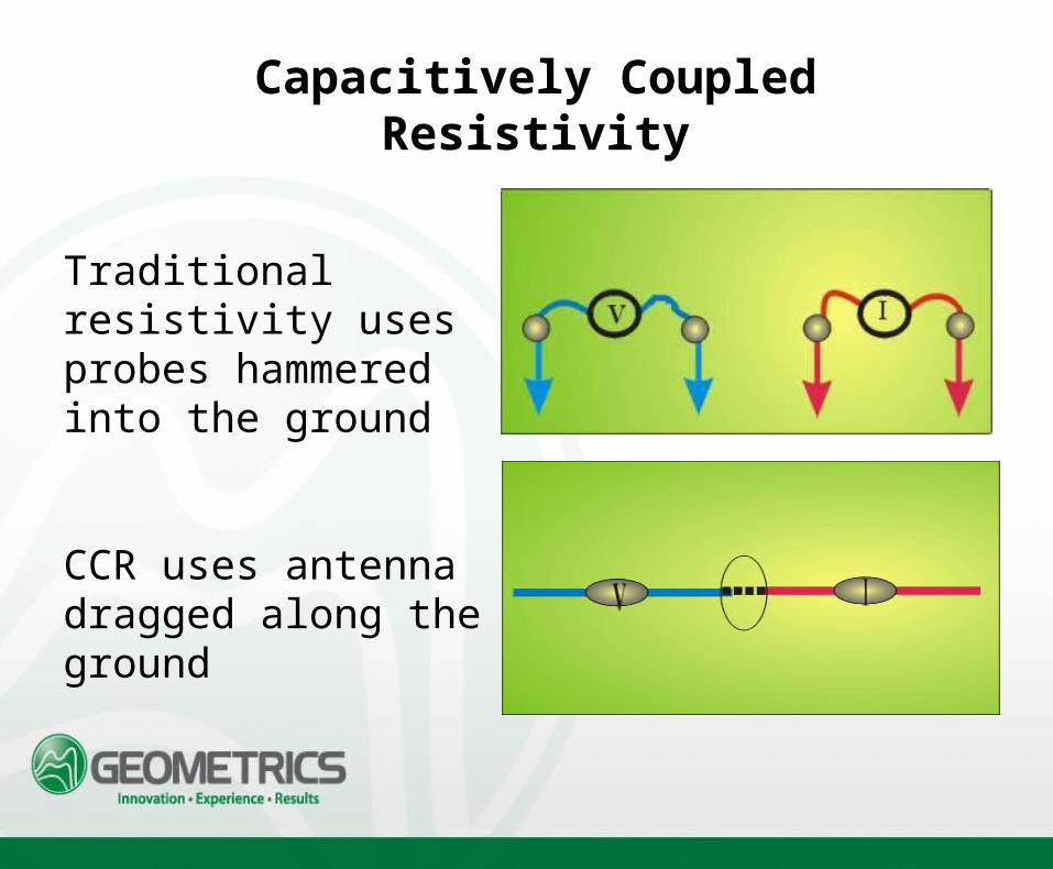
Capacitively Coupled Resistivity

Traditional resistivity uses probes hammered into the ground

CCR uses antenna dragged along the ground

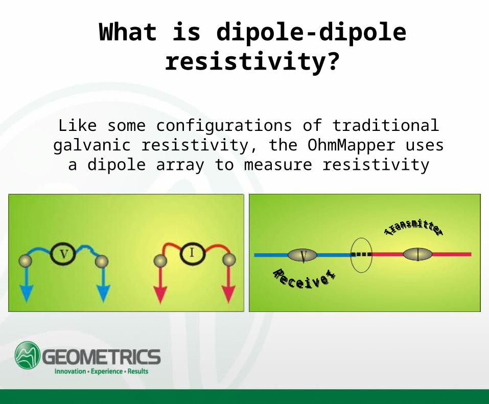
What is dipole-dipole resistivity?

Like some configurations of traditional galvanic resistivity, the OhmMapper uses a dipole array to measure resistivity

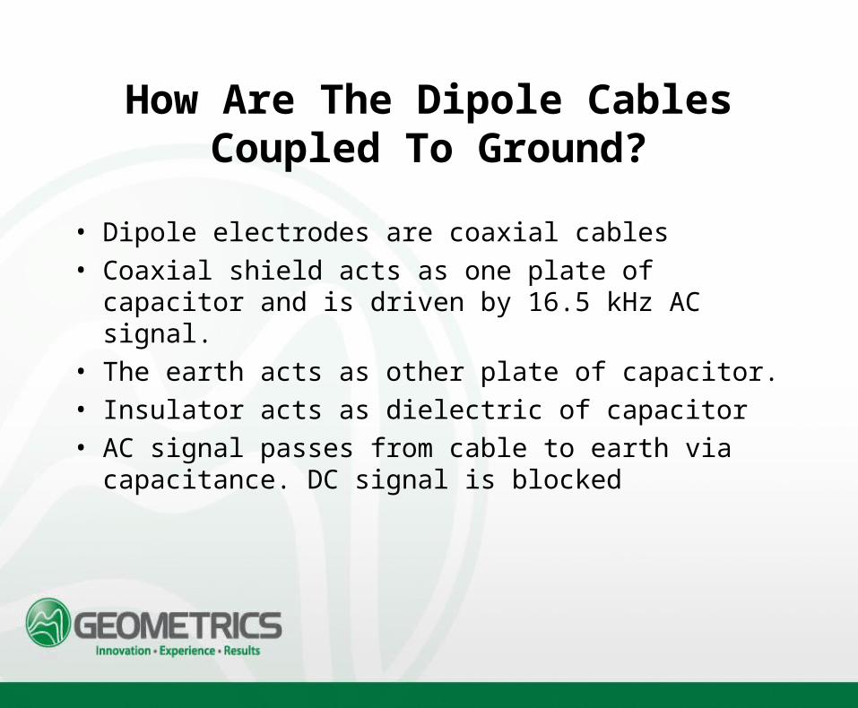
How Are The Dipole Cables Coupled To Ground?

• Dipole electrodes are coaxial cables• Coaxial shield acts as one plate of capacitor and is driven by

16.5 kHz AC signal.• The earth acts as other plate of capacitor.• Insulator acts as dielectric of capacitor• AC signal passes from cable to earth via capacitance. DC signal

is blocked

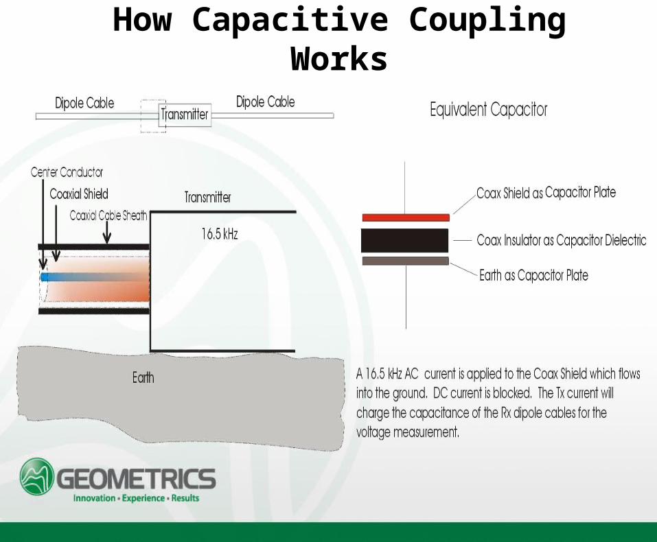
How Capacitive Coupling Works

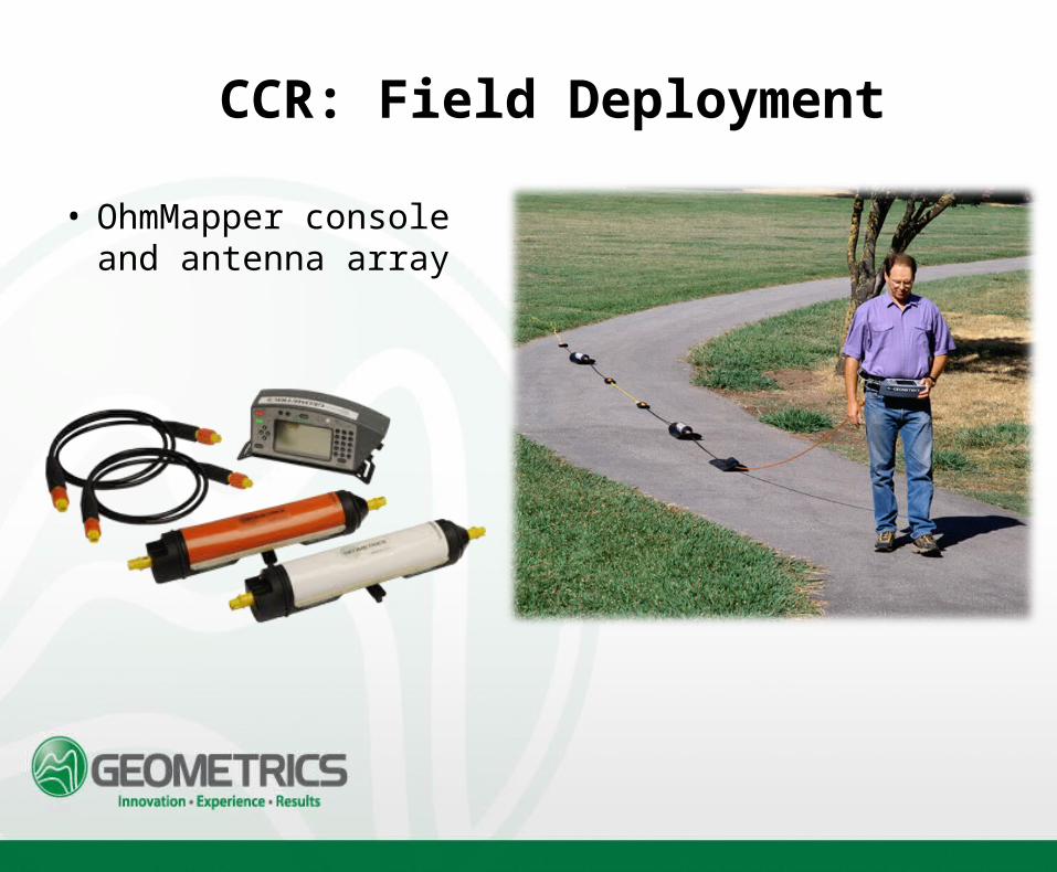
CCR: Field Deployment

• OhmMapper console and antenna array

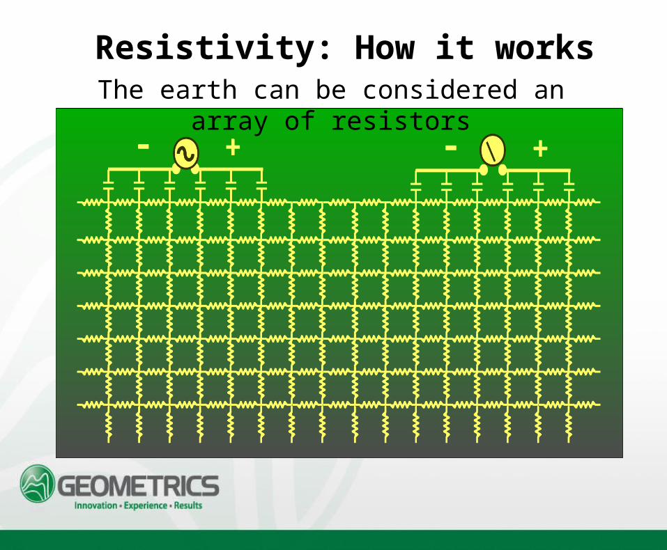
Resistivity: How it worksThe earth can be considered an array of resistors

How Does The Receiver Know What Current The Transmitter Is Generating?

The OhmMapper uses a patented modulation scheme, in which the

transmitter’s AC current is communicated by a lower-frequency

signal. In this way the transmitter current is encoded in the transmitter

signal itself.

At the receiver the measured voltage is demodulated to “decode” the

transmitter signal and thus extract the current information.

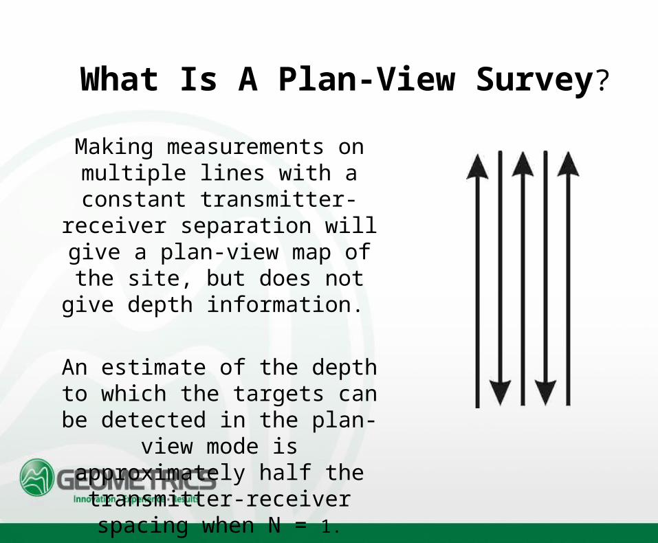
What Is A Plan-View Survey?

Making measurements on multiple lines with a constant transmitter-receiver

separation will give a plan-view map of the site, but does not give depth

information.

An estimate of the depth to which the targets can be detected in the plan-view

mode is approximately half the transmitter-receiver spacing when N = 1.

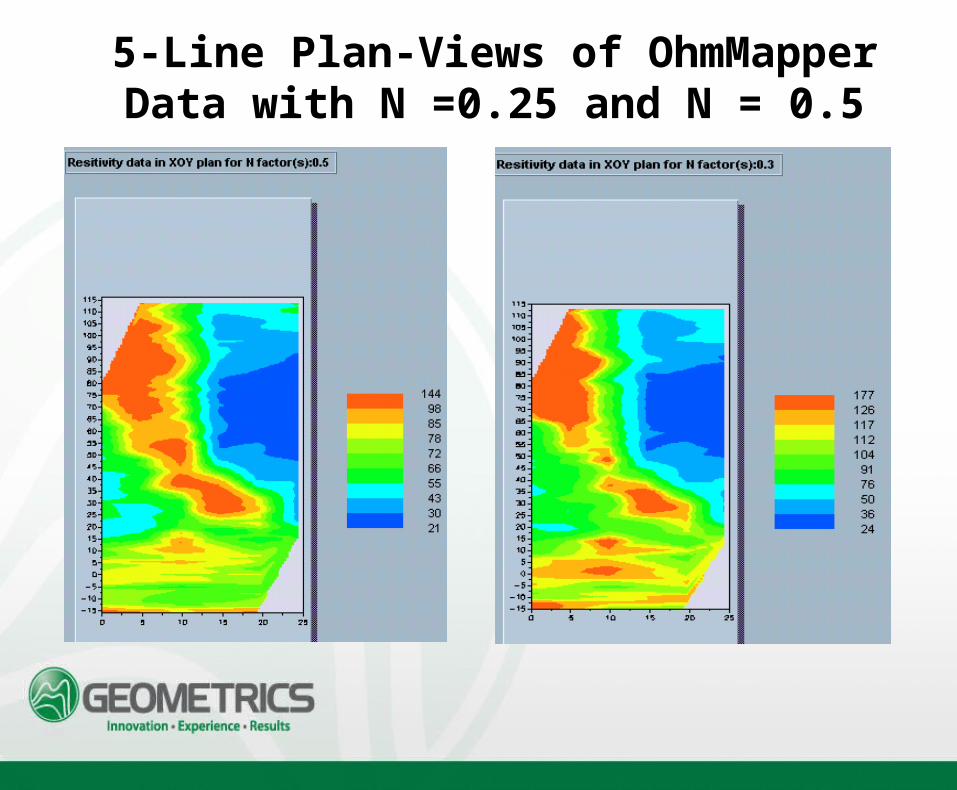
5-Line Plan-Views of OhmMapper Data with N =0.25 and N = 0.5

How Is A Depth Section Made With Traditional Galvanically-Coupled

Dipole-dipole Resistivity?

•Probes hammered into the ground at predetermined distances•Probes moved after each measurement•Occasionally a switch system used to select probes•Very time consuming!

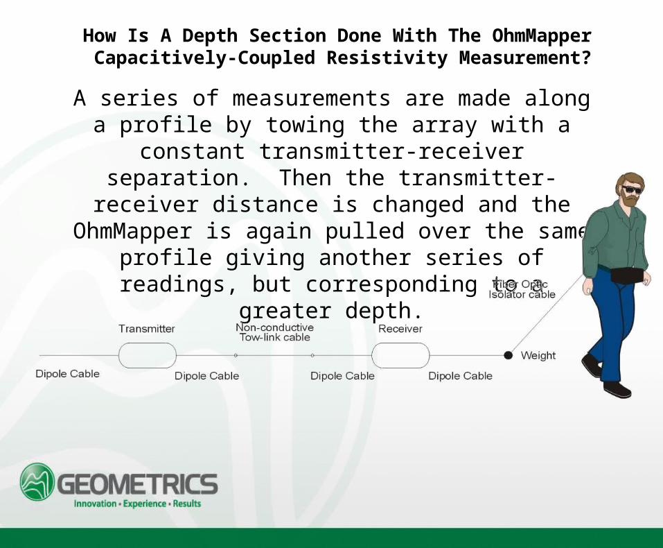
How Is A Depth Section Done With The OhmMapper Capacitively-Coupled Resistivity Measurement?

A series of measurements are made along a profile by towing the array with a constant transmitter-receiver separation. Then the transmitter-receiver distance is changed and the OhmMapper is

again pulled over the same profile giving another series of readings, but corresponding to a greater depth.

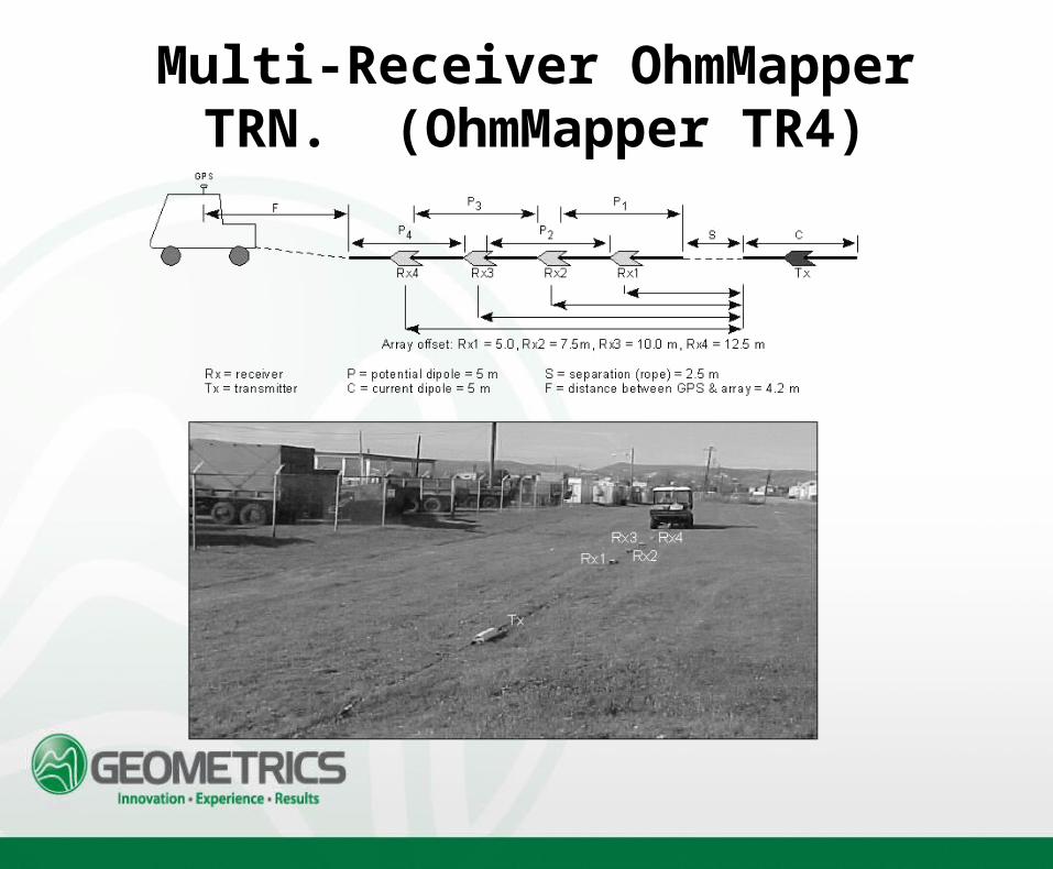
Multi-Receiver OhmMapper TRN. (OhmMapper TR4)

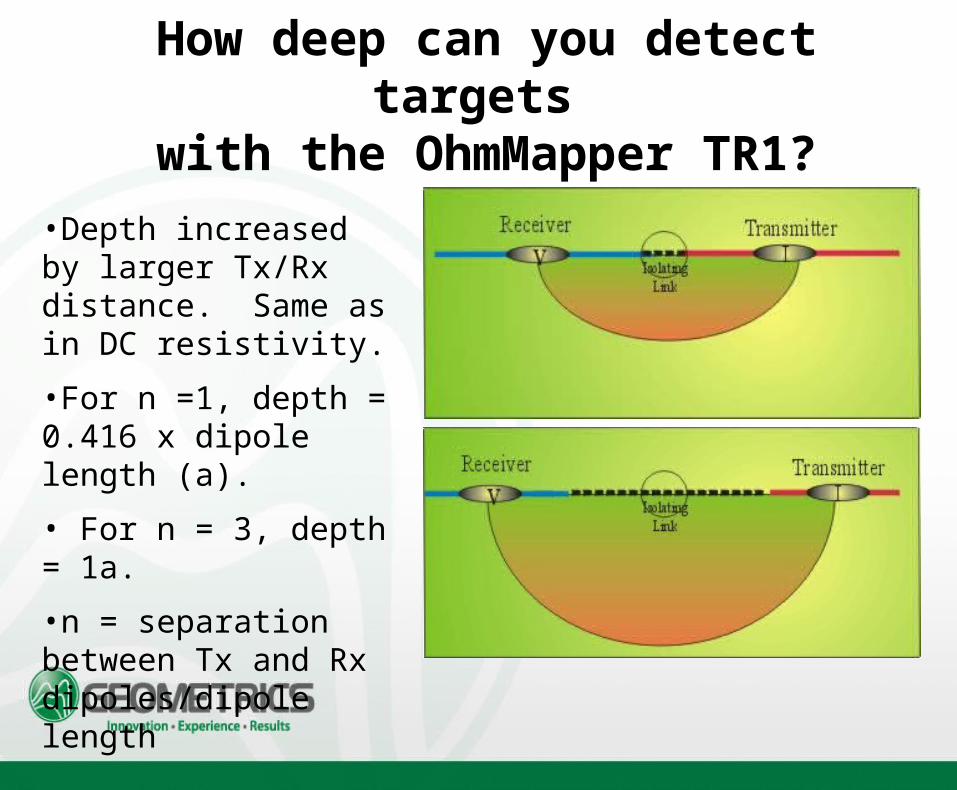
How deep can you detect targets with the OhmMapper TR1?

•Depth increased by larger Tx/Rx distance. Same as in DC resistivity.

•For n =1, depth = 0.416 x dipole length (a).

• For n = 3, depth = 1a.

•n = separation between Tx and Rx dipoles/dipole length

Depth of Investigation

•Although the array geometry determines depth of investigation practical limits of depth of are determined by ground resistivity.

•Signal attenuated by 1/r3

•By Ohm’s Law V=IR therefore high R gives high signal V. Receiver can detect transmitter at long Tx/Rx separation in resistive earth. Low R gives small V so transmitter must be near receiver in conductive earth.

•Can get more separation and therefore greater depth in resistive earth.

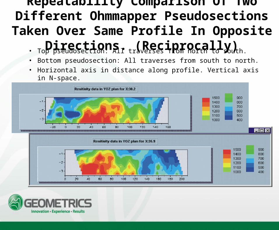
Repeatability Comparison Of Two Different Ohmmapper Pseudosections Taken Over Same Profile

In Opposite Directions. (Reciprocally)• Top pseudosection: All traverses from north to south. • Bottom pseudosection: All traverses from south to north.• Horizontal axis in distance along profile. Vertical axis in N-space.

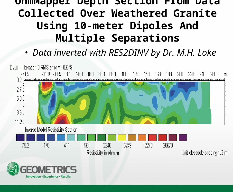
OhmMapper Depth Section From Data Collected Over Weathered Granite Using 10-meter Dipoles

And Multiple Separations

• Data inverted with RES2DINV by Dr. M.H. Loke

Detection of Cavity in Karst

The following slides show a test in which an OhmMapper was dragged over a known cavity. The position of the

cavity matches well with the high-resistivity target in the depth section.

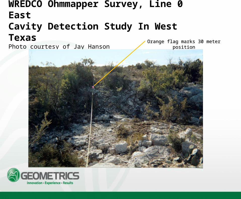
WREDCO Ohmmapper Survey, Line 0 EastCavity Detection Study In West TexasPhoto courtesy of Jay Hanson

Orange flag marks 30 meter positionOrange flag marks 30 meter position

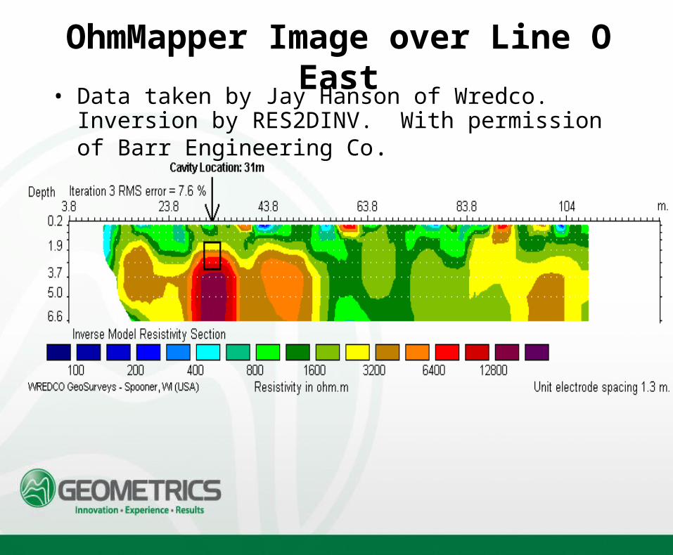
OhmMapper Image over Line O East• Data taken by Jay Hanson of Wredco. Inversion by RES2DINV.

With permission of Barr Engineering Co.

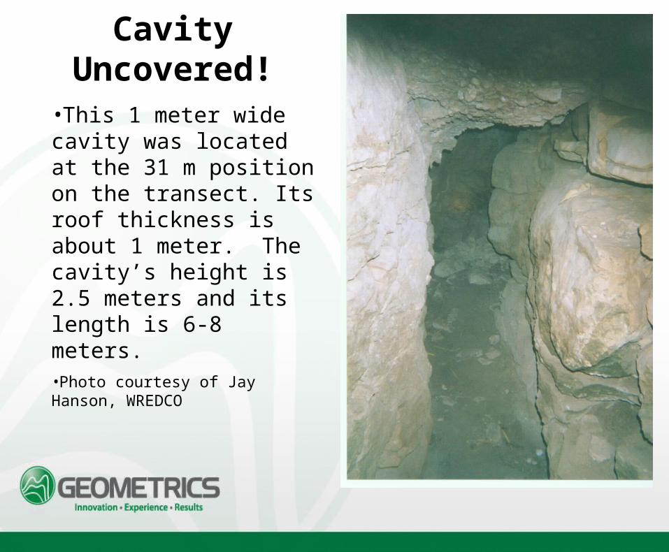
Cavity Uncovered!

•This 1 meter wide cavity was located at the 31 m position on the transect. Its roof thickness is about 1 meter. The cavity’s height is 2.5 meters and its length is 6-8 meters. •Photo courtesy of Jay Hanson, WREDCO

Litigation Survey For Cavity Under Private House

The next slide shows the results of a survey done to determine the cause of damage to a home in Florida. The results from an OhmMapper survey was evidence that proved the damage was the result of a karst cavity under the house. See details in St. Petersburg Times article at web site www.sptimes.com and search on OhmMapper.

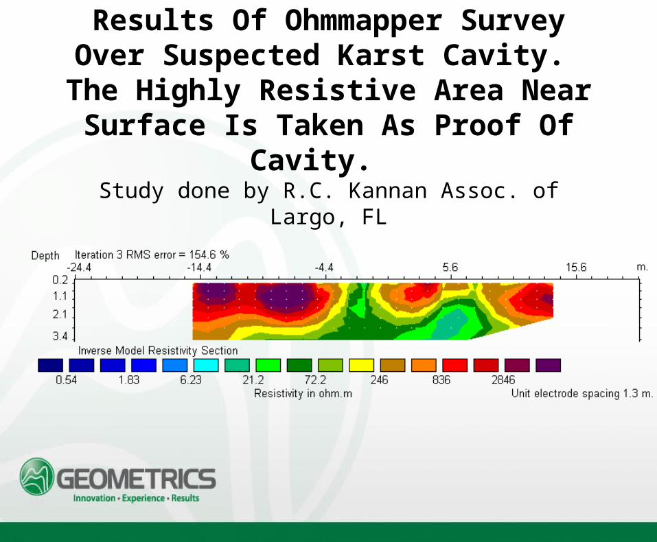
Results Of Ohmmapper Survey Over Suspected Karst Cavity. The Highly Resistive Area Near Surface Is Taken

As Proof Of Cavity. Study done by R.C. Kannan Assoc. of Largo, FL

Bedrock Mapping

The following slide shows the results of an OhmMapper survey to map

bedrock. The conductive (blue) top layer is taken to correspond to the

sedimentary layer. This was confirmed by the observation that

the areas on the depth section showing no sediments generally

corresponded to rock outcropping.

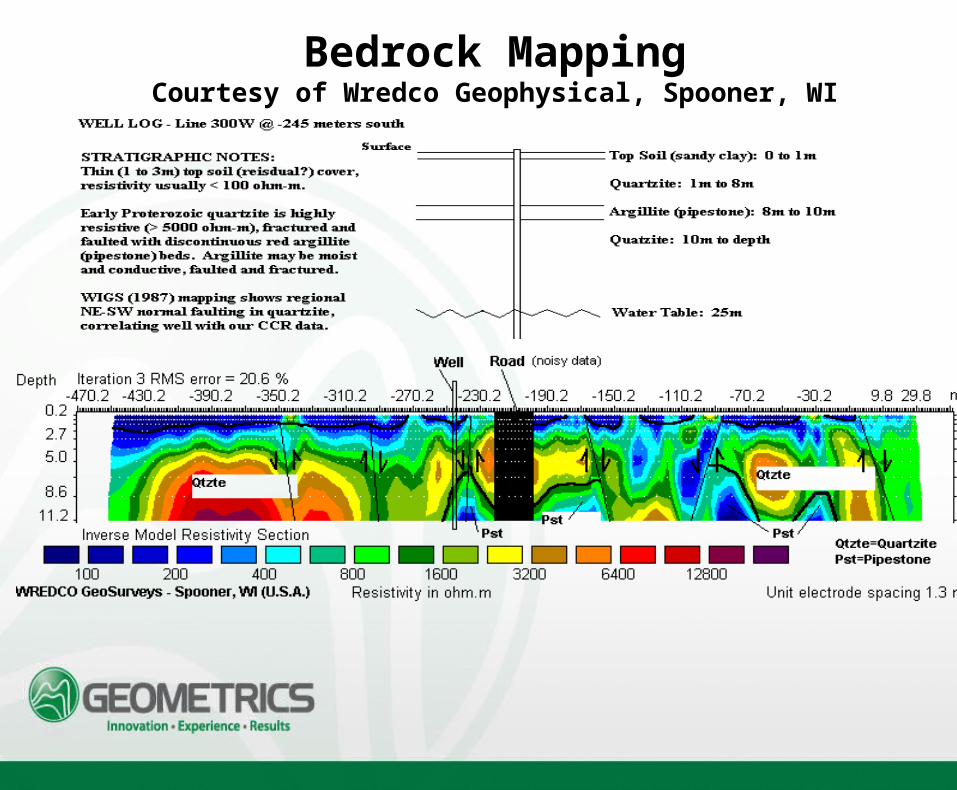
Bedrock MappingCourtesy of Wredco Geophysical, Spooner, WI

Agricultural Soil Mapping

The next slide shows the results of a US Dept. of Agriculture OhmMapper survey in an experimental corn field. Harvest

productivity was compared to depth of top soil. Those areas that show very shallow top soil map well to low-productivity

areas. Deep top soil, as mapped on the depth section, corresponded to higher productivity.

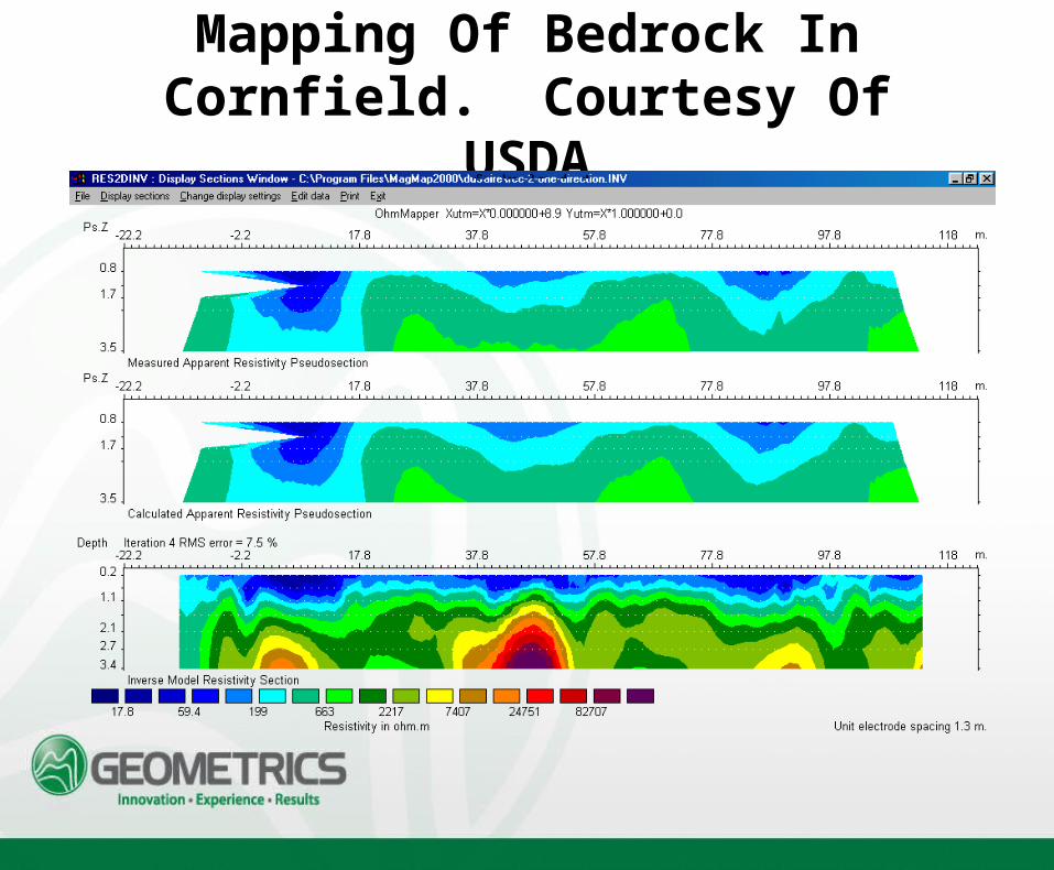
Mapping Of Bedrock In Cornfield. Courtesy Of USDA

Mapping Clay Lense

The following data was collected by Bucknell University students and professor with an OhmMapper TR1. The known geology is

approximately 3m of moderately resistive loose sandy soil followed by 4 meters of more conductive

clay, then resistive base rock.

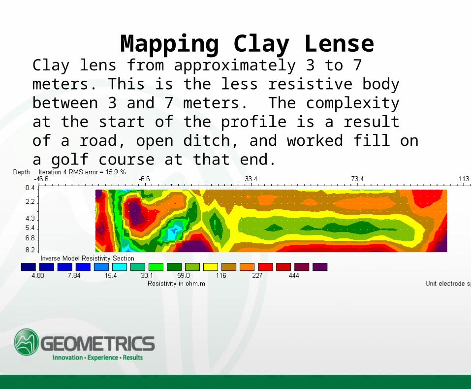
Clay lens from approximately 3 to 7 meters. This is the less resistive body between 3 and 7 meters. The complexity at the start of the profile is a result of a road, open ditch, and worked fill on a golf course at that end.

Mapping Clay Lense

New Road Construction Site - DOT Survey

• NDT Corporation participated with the Federal Highway Administration, Massachusetts Highway Department and Geometrics in a demonstration project to evaluate the effectiveness of Geometric’s OhmMapper system to locate and define the lateral and vertical extents of peat deposits along a highway construction right of way. The test area was in Carver, Massachusetts on a section of Route 44 that is currently under construction.

New Road Construction Site - DOT Survey

• Peat was excavated to depths varying from 15 to 30 feet and replaced with sand. Borings indicated peat deposits below the sand fill. A resistivity survey was conducted in an area where borings indicated the presence of peat. After completion of the resistivity survey the area was excavated and the peat deposits mapped for comparison with resistivity survey results. Soil, ground water, and peat samples were obtained from the site materials for laboratory resistivity tests.

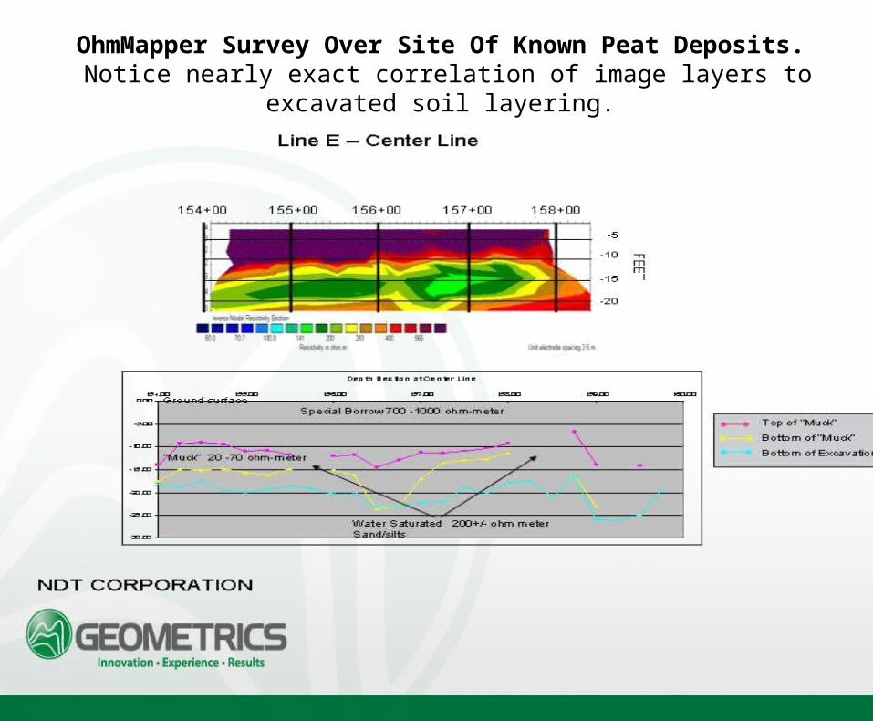
OhmMapper Survey Over Site Of Known Peat Deposits. Notice nearly exact correlation of image layers to excavated soil layering.

Survey of River Levee in Japan

• An OhmMapper TR5 was used to survey a 1.3 km segment of a river levee near Tsukuba, Japan. The purpose of the survey was to estimate the integrity of the levee structure and view the interface between the levee and the underlying clay bed.

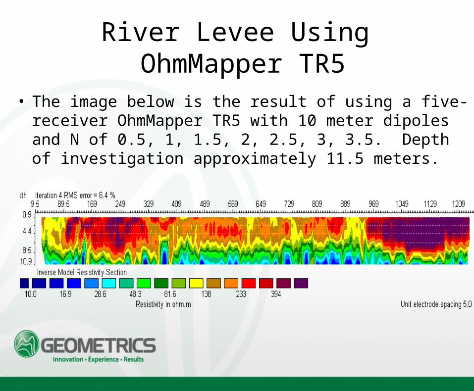
River Levee Using OhmMapper TR5

• The image below is the result of using a five-receiver OhmMapper TR5 with 10 meter dipoles and N of 0.5, 1, 1.5, 2, 2.5, 3, 3.5. Depth of investigation approximately 11.5 meters.

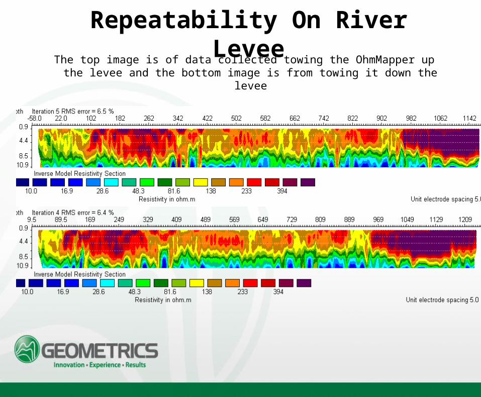
Repeatability On River LeveeThe top image is of data collected towing the OhmMapper up the

levee and the bottom image is from towing it down the levee

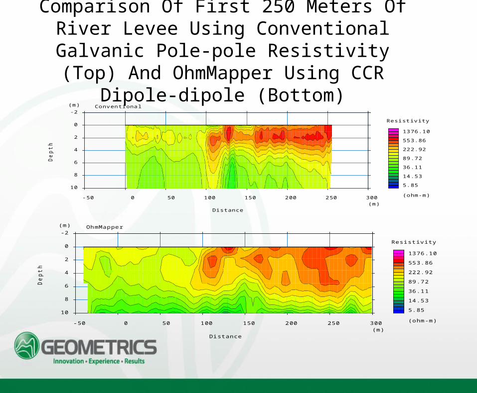
Comparison Of First 250 Meters Of River Levee Using Conventional Galvanic Pole-pole

Resistivity (Top) And OhmMapper Using CCR Dipole-dipole (Bottom)

10

8

6

4

2

0

-2

Depth

(m)

-50 0 50 100 150 200 250 300(m)

Distance

Conventional

(ohm-m)

Resistivity

5.85

14.53

36.11

89.72

222.92

553.86

1376.10

10

8

6

4

2

0

-2

Depth

(m)

-50 0 50 100 150 200 250 300(m)

Distance

OhmMapper

(ohm-m)

Resistivity

5.85

14.53

36.11

89.72

222.92

553.86

1376.10

Tracking Fracture Zones

• The next slides shows the results of multiple profiles done with an OhmMapper. The contractor interpreted the continuation of similar resistivities from line to line as indicating the strike of geologic structures, perhaps indicating the presence and direction of fracture zones.

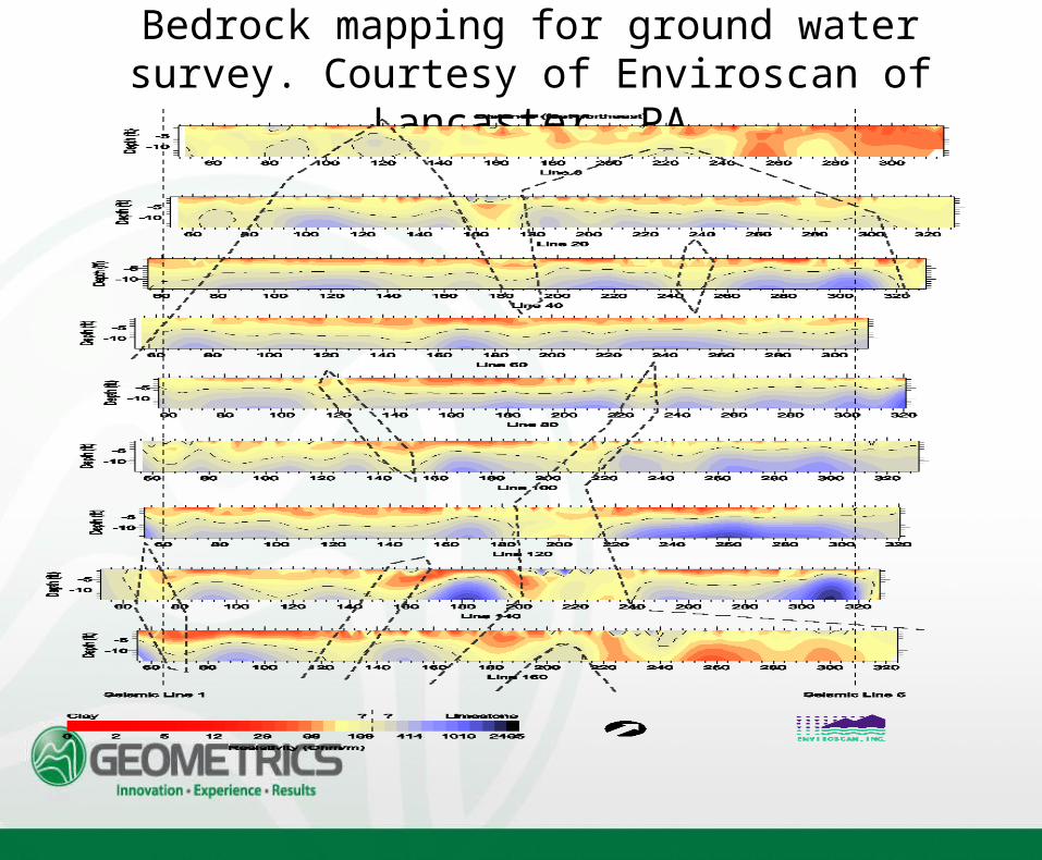
Bedrock mapping for ground water survey. Courtesy of Enviroscan of

Lancaster, PA

Fracture Zones #2

• The following slide is another example of possible fracture zones shown in multiple OhmMapper resistivity profiles.

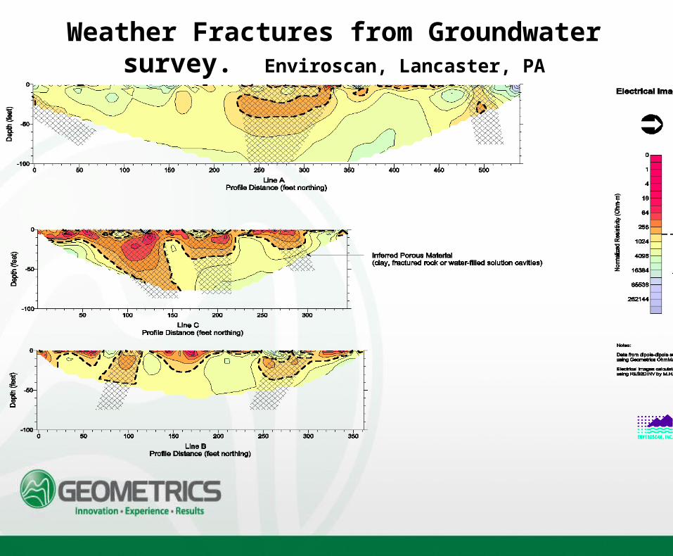
Weather Fractures from Groundwater survey. Enviroscan, Lancaster, PA

Test Image Of Known Culvert

• The next two slides show a culvert detected with the OhmMapper using both a set of 5-meter dipoles and an experimental set of 1.5 meter dipoles.

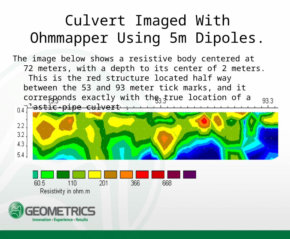
Culvert Imaged With Ohmmapper Using 5m Dipoles.

The image below shows a resistive body centered at 72 meters, with a depth to its center of 2 meters. This is the red structure located half way between the 53 and 93 meter tick marks, and it corresponds exactly with the true location of a plastic-pipe culvert .

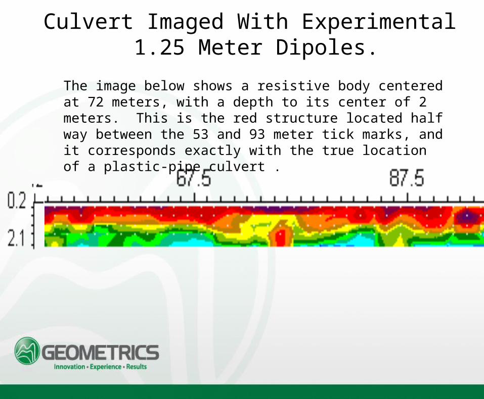
Culvert Imaged With Experimental 1.25 Meter Dipoles.

The image below shows a resistive body centered at 72 meters, with a depth to its center of 2 meters. This is the red structure located half way between the 53 and 93 meter tick marks, and it corresponds exactly with the true location of a plastic-pipe culvert .

Archeological Surveying

The next slide was taken over the location of a suspected Roman Amphitheater in England. The survey was run using multiple parallel lines with a single Tx/Rx separation in order to do a fast reconnaissance of the area. Although the site has not yet been excavated the circular feature shown in the plan view map indicates the presence of the walls of the amphitheater.

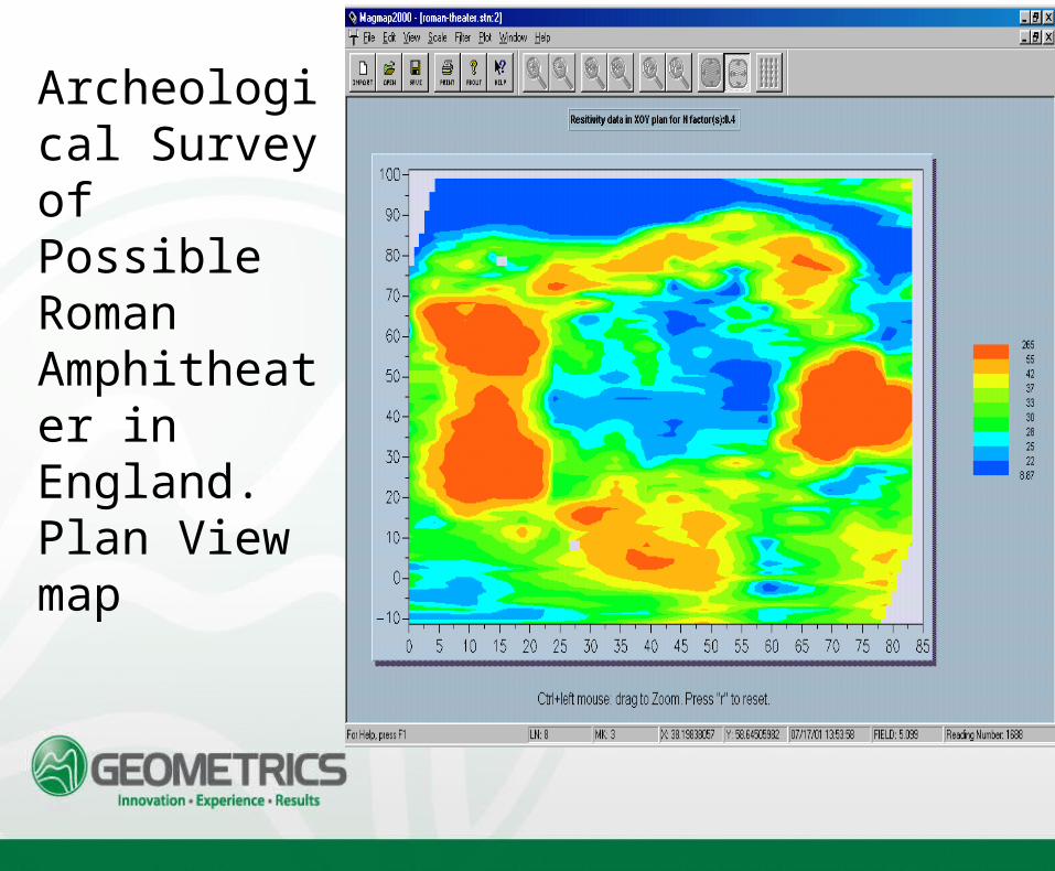
Archeological Survey of Possible Roman Amphitheater in England. Plan View map

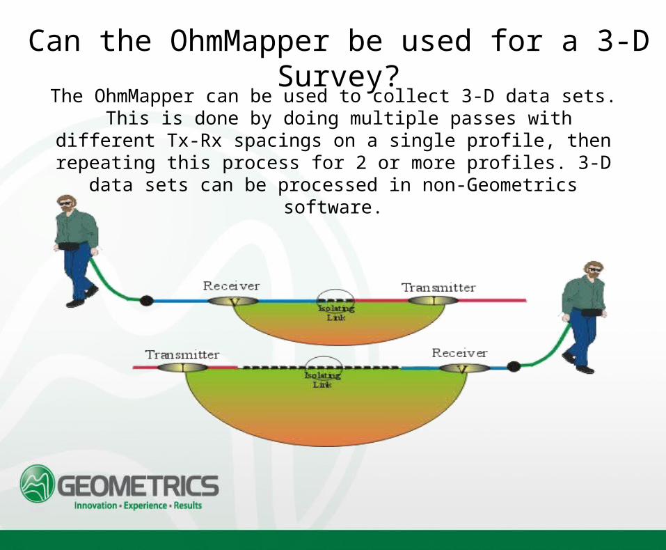
Can the OhmMapper be used for a 3-D Survey?The OhmMapper can be used to collect 3-D data sets. This is done by doing multiple passes with different Tx-Rx spacings on a single profile, then repeating this process for 2 or more profiles. 3-D data sets can be processed in non-Geometrics

software.

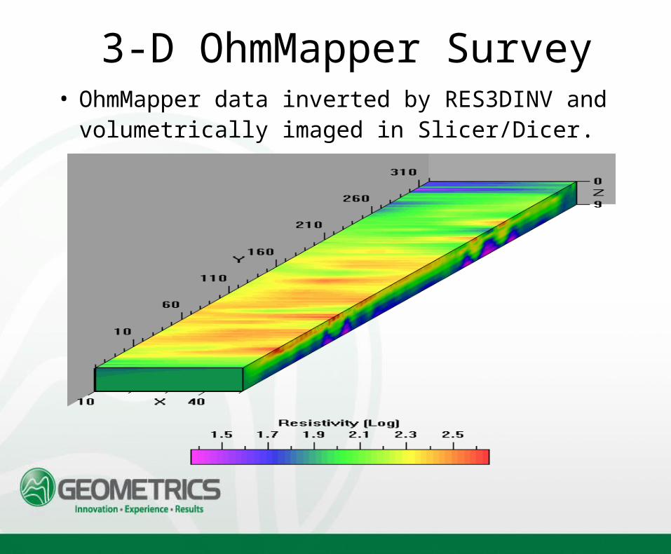
3-D OhmMapper Survey• OhmMapper data inverted by RES3DINV and

volumetrically imaged in Slicer/Dicer.

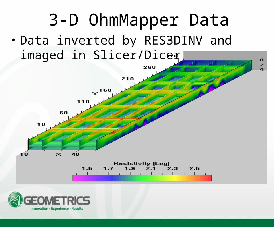
3-D OhmMapper Data • Data inverted by RES3DINV and imaged in Slicer/Dicer

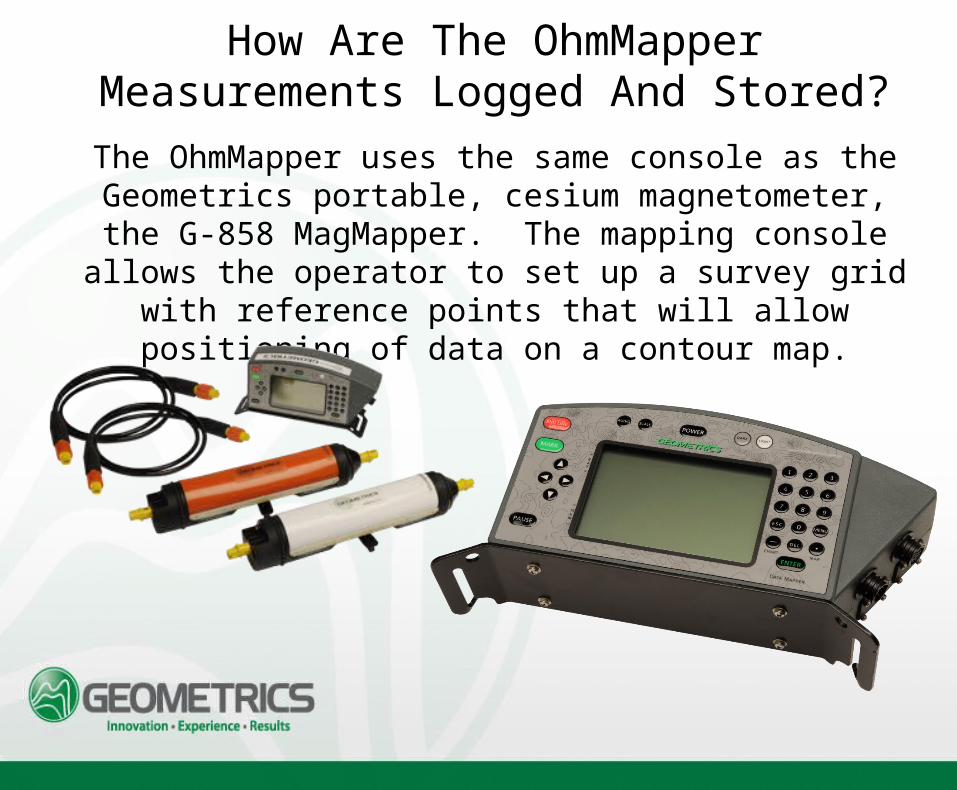
How Are The OhmMapper Measurements Logged And Stored?

The OhmMapper uses the same console as the Geometrics portable, cesium magnetometer, the G-858 MagMapper. The mapping console

allows the operator to set up a survey grid with reference points that will allow positioning of data on a contour map.

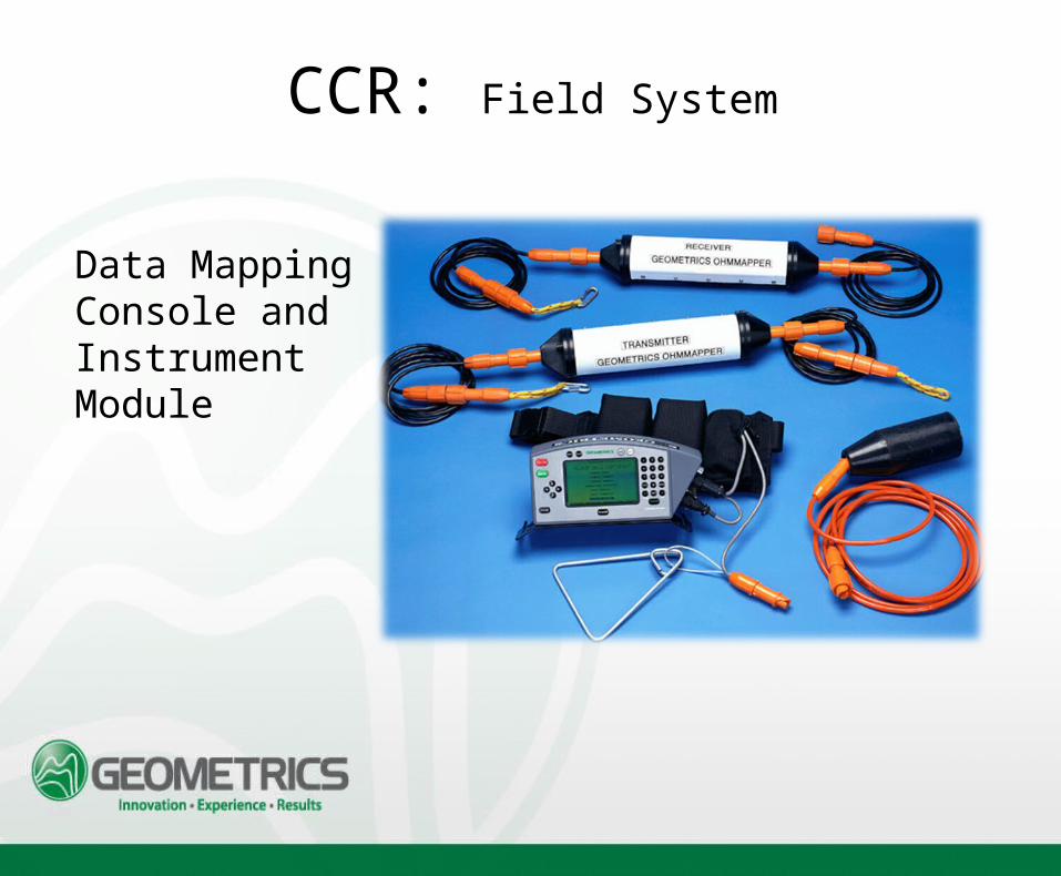
CCR: Field System

Data Mapping Console and Instrument Module

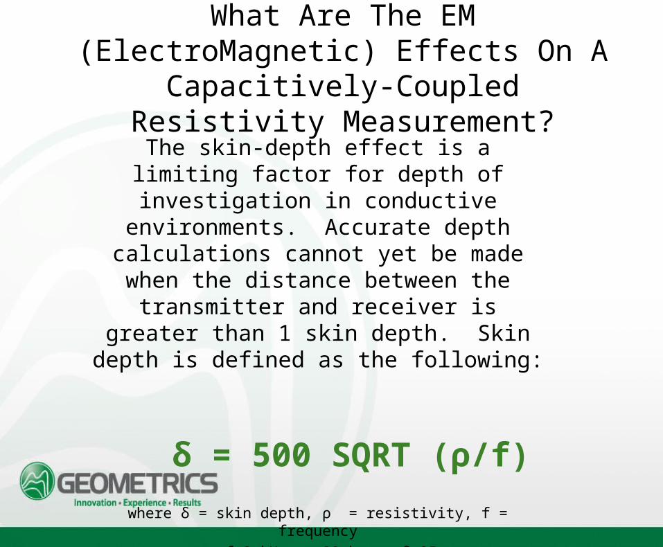
What Are The EM (ElectroMagnetic) Effects On A Capacitively-Coupled

Resistivity Measurement?

The skin-depth effect is a limiting factor for depth of investigation in conductive environments. Accurate

depth calculations cannot yet be made when the distance between the transmitter and receiver is greater than 1 skin depth. Skin depth is defined as the following:

δ = 500 SQRT (ρ/f)

where δ = skin depth, ρ = resistivity, f = frequencyeg: f=8 kHz, ρ=20ohm-m, δ=25m

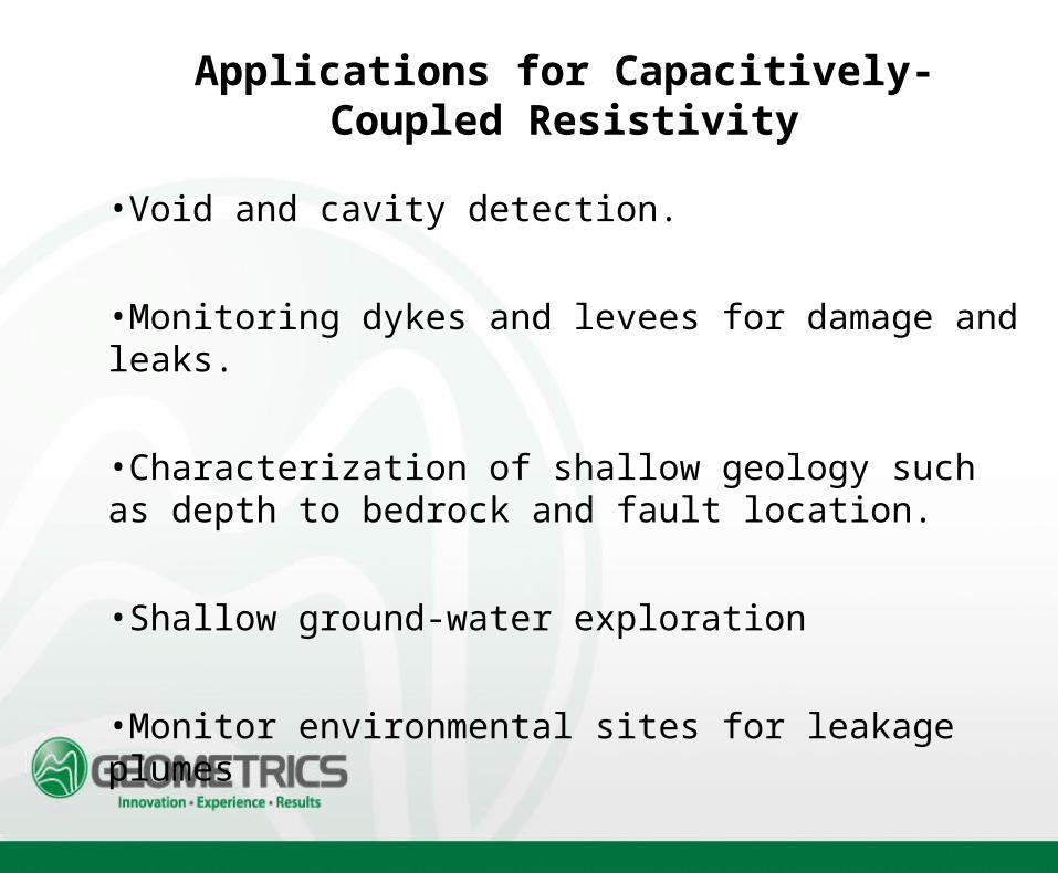
Applications for Capacitively-Coupled Resistivity

•Void and cavity detection.

•Monitoring dykes and levees for damage and leaks.

•Characterization of shallow geology such as depth to bedrock and fault location.

•Shallow ground-water exploration

•Monitor environmental sites for leakage plumes

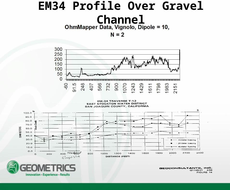
EM34 Profile Over Gravel Channel

Comparison Of Galvanic Dipole Results With Ohmmapper Results

• On the next slide, the data on the right was taken with the OhmMapper and inverted with software developed by KIGAM in Korea. The data set on the left was taken at the same place, but with a traditional galvanic, multi-electrode resistivity meter. The color scales are identical.

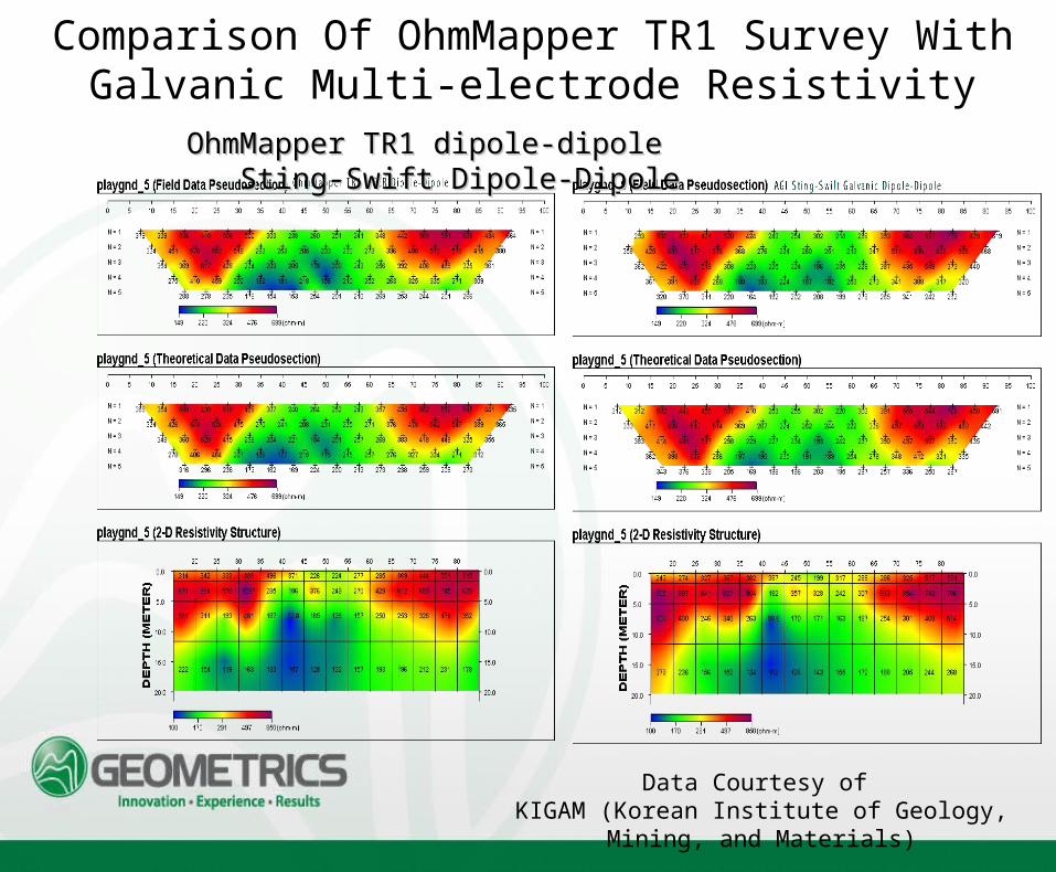
Comparison Of OhmMapper TR1 Survey With Galvanic Multi-electrode Resistivity

Data Courtesy of KIGAM (Korean Institute of Geology, Mining, and Materials)

OhmMapper TR1 dipole-dipoleOhmMapper TR1 dipole-dipole Sting-Swift Dipole-Dipole Sting-Swift Dipole-Dipole

Comparison Of Galvanic Multi-electrode Measurements With Ohmmapper #2.

• This next slide compares an area of overlap of a multi-electrode, galvanic survey and an OhmMapper survey. The scales are the same. Although there is only about 40 meters where the two surveys overlapped the depth sections show close similarities. The color scales are identical.

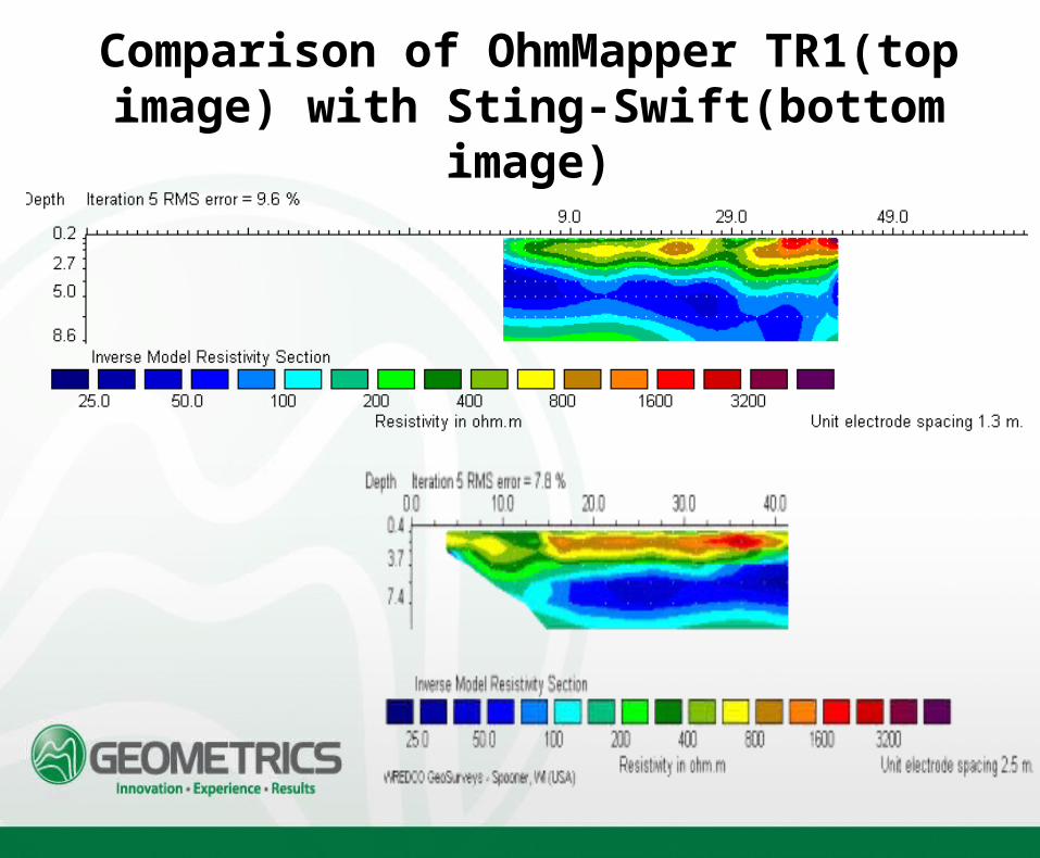
Comparison of OhmMapper TR1(top image) with Sting-Swift(bottom image)

OhmMapper and GPR Comparison

The following example shows the results of an OhmMapper 2-D survey carried out over the same profile where a GPR survey had been done previously. Note the remarkable one-to-one correspondence of the layer contours in the two images. Data courtesy of Subsurface Evaluations, Inc. of Tampa, FL

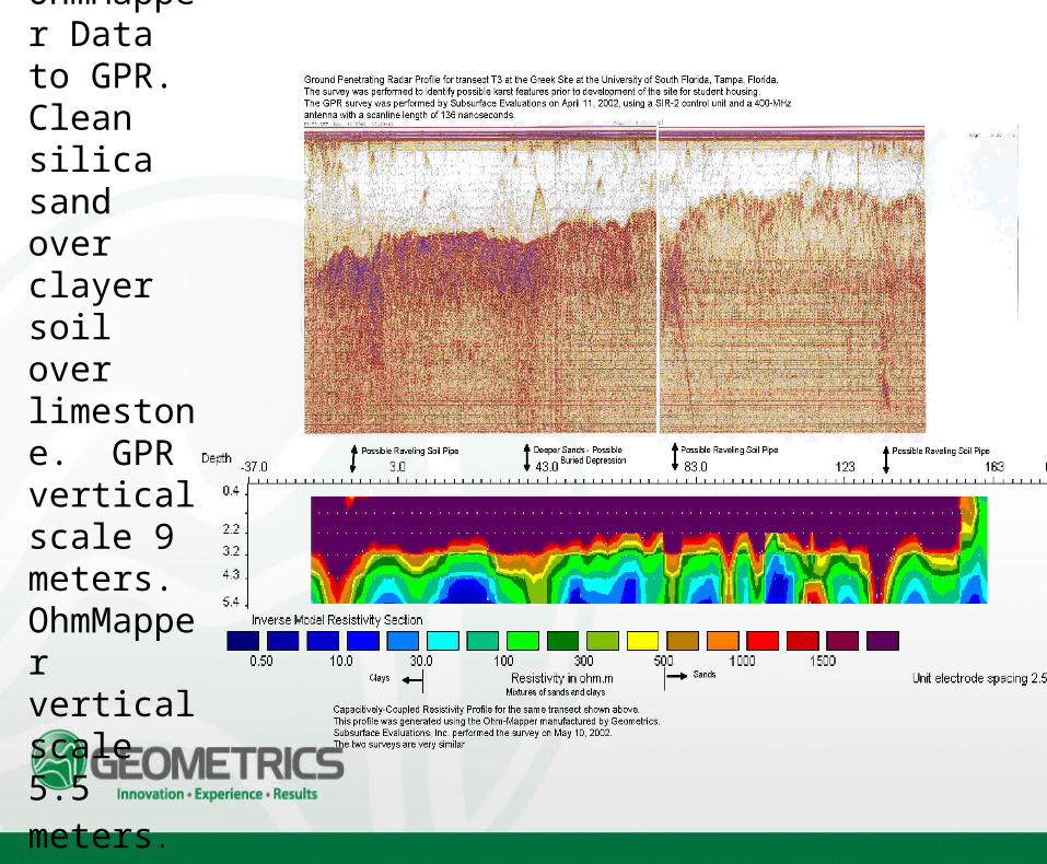
Comparison of OhmMapper Data to GPR. Clean silica sand over clayer soil over limestone. GPR vertical scale 9 meters. OhmMapper vertical scale 5.5 meters.

Comparison of OhmMapper to EM31

• The following slide shows a comparison of planview maps from EM31 and OhmMapper surveys over the same area. Note the well defined open bedding planes seen in the OhmMapper data. The depth of investigation may not be the same for both data sets, but an attempt was made to approximate similar depths for both maps.

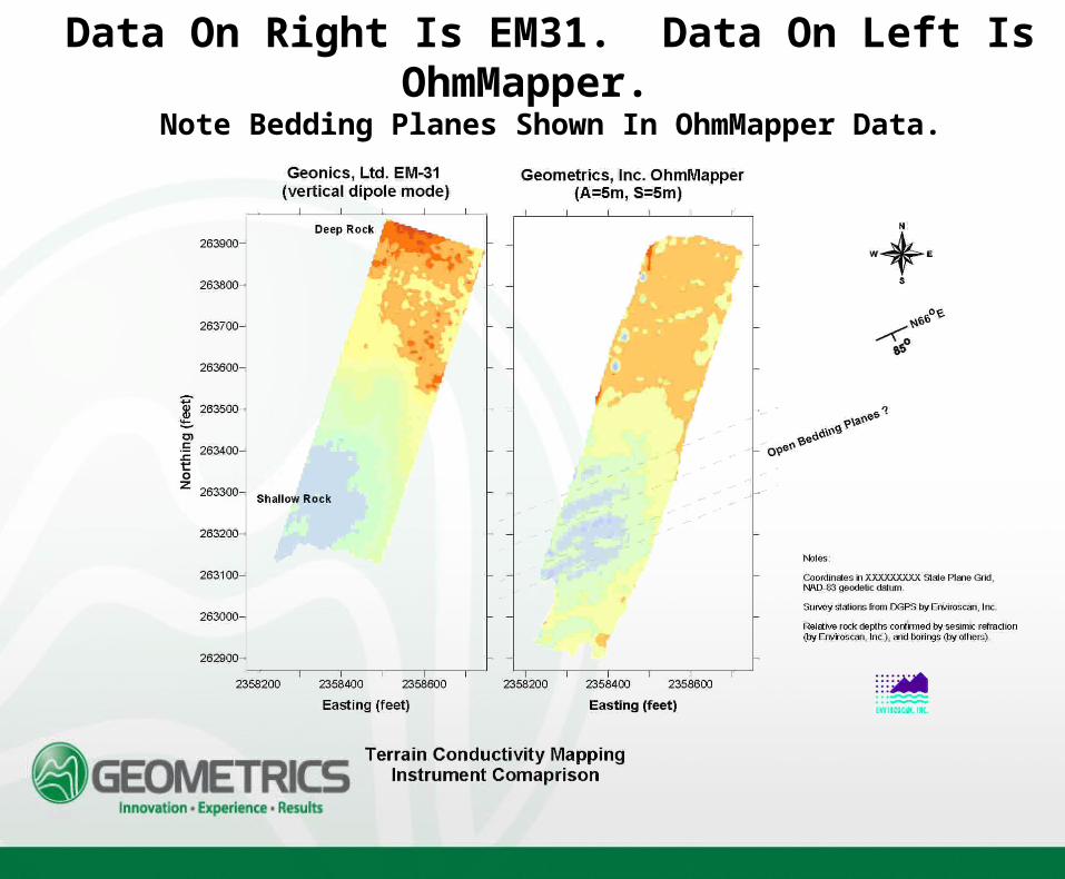
Data On Right Is EM31. Data On Left Is OhmMapper.

Note Bedding Planes Shown In OhmMapper Data.

Comparison of OhmMapper Profile to Microgravity

• The next three slides show correlation between the results of microgravity surveys and OhmMapper TR1 profiles over the same area. Geometrics thanks Enviroscan, Inc. of Lancaster, PA for the use of this data.

Microgravity and OhmMapper Comparison #1

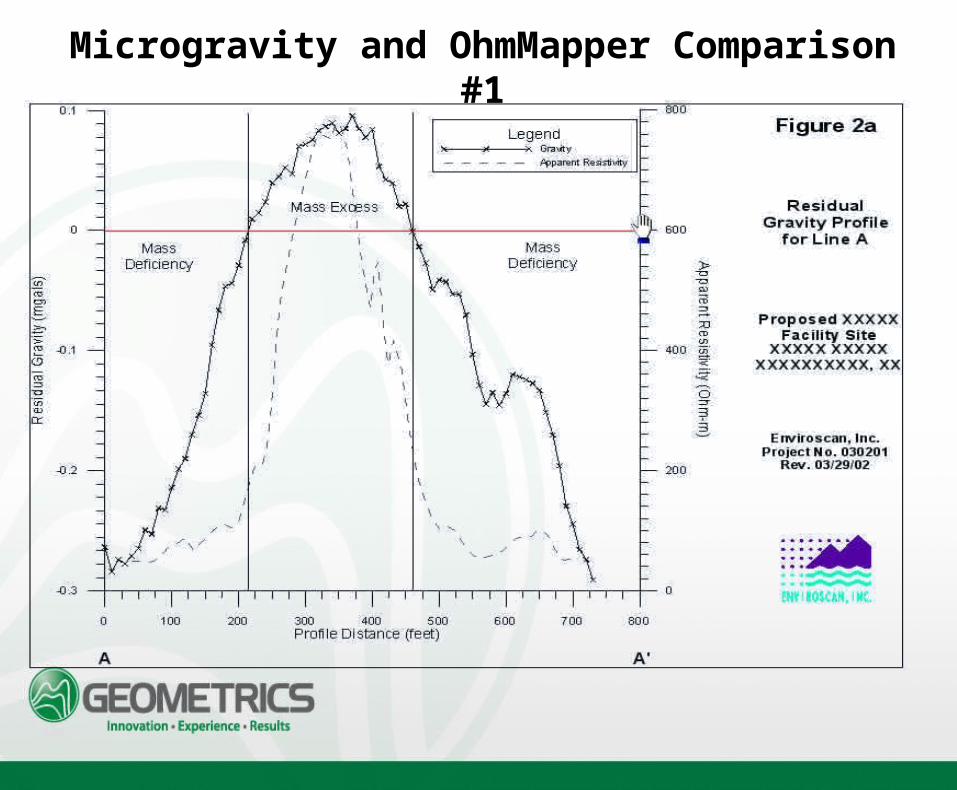
Microgravity and OhmMapper Comparison #2

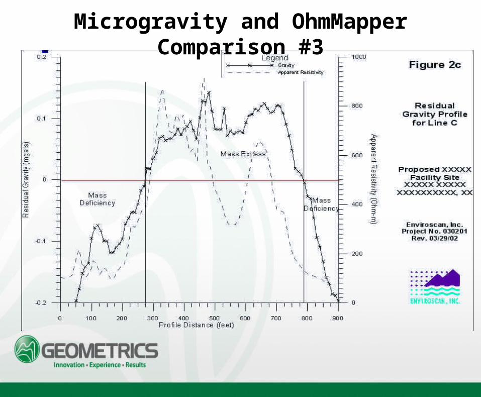
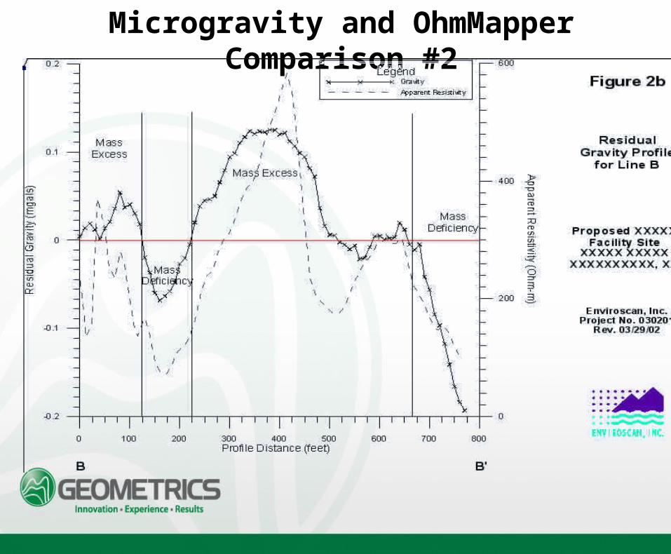
Microgravity and OhmMapper Comparison #3

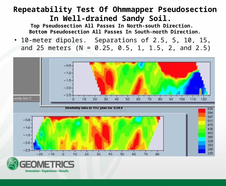
Repeatability Test Of Ohmmapper PseudosectionIn Well-drained Sandy Soil.

Top Pseudosection All Passes In North-south Direction. Bottom Pseudosection All Passes In South-north Direction.

• 10-meter dipoles. Separations of 2.5, 5, 10, 15, and 25 meters (N = 0.25, 0.5, 1, 1.5, 2, and 2.5)

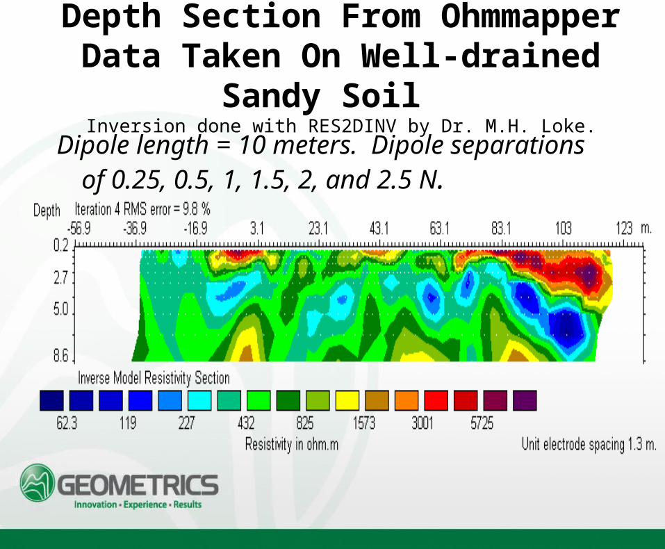
Depth Section From Ohmmapper Data Taken On Well-drained Sandy Soil

Inversion done with RES2DINV by Dr. M.H. Loke.

Dipole length = 10 meters. Dipole separations of 0.25, 0.5, 1, 1.5, 2, and 2.5 N.

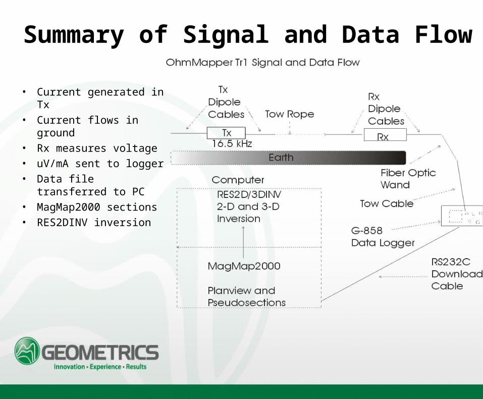
Summary of Signal and Data Flow

• Current generated in Tx• Current flows in ground• Rx measures voltage • uV/mA sent to logger• Data file transferred to

PC• MagMap2000 sections• RES2DINV inversion

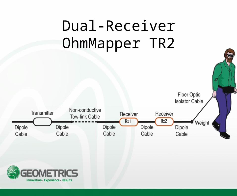
Dual-Receiver OhmMapper TR2

Comparison Of TR2 And TR1 Results

• The pseudosections on the right were generated with a TR2. Those on the left were generated with TR1 data taken over the same profile lines.

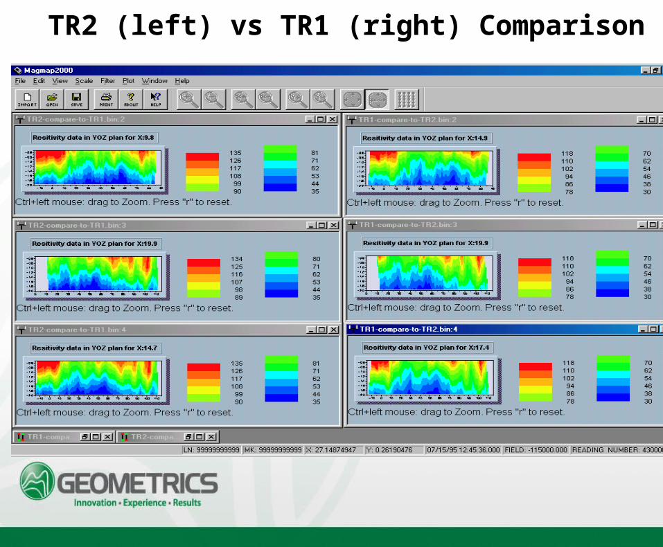
TR2 (left) vs TR1 (right) Comparison

Advantages of Capacitively-Coupled Resistivity

• Fast - data can be collected at a walking pace• Portable - one man operation• Automatic - can be vehicle towed• Flexible - can be used for profiling and sounding• Versatile - used an accessory for G-858 cesium

magnetometer• Low power - works in very high resistivity environments

without supplemental power