Reserve Bank of Australia

Reserve Bank of AustraliaEconomic Research Department

2007

-11

RESEARCHDISCUSSIONPAPER

Global Imbalances and the Global Saving Glut – A Panel Data Assessment

Anthony Legg, Nalini Prasad and Tim Robinson

RDP 2007-11

GLOBAL IMBALANCES AND THE GLOBAL SAVING GLUT –A PANEL DATA ASSESSMENT

Anthony Legg, Nalini Prasad and Tim Robinson

Research Discussion Paper 2007-11

November 2007

Economic Research Department Reserve Bank of Australia

We would like to thank Andrew Stone who contributed to the original ideas and early work for this paper. We would also like to thank Christopher Kent, David Orsmond, Adam Cagliarini, Malcolm Edey and David Vines for helpful comments, and Tim Callen and Mahnaz Hemmati at the International Monetary Fund for providing data. The views expressed herein are those of the authors and do not necessarily reflect those of the Reserve Bank of Australia.

Authors: prasadn or robinsont at domain rba.gov.au

Economic Publications: ecpubs@rba.gov.au

i

Abstract

Since the late 1990s there have been substantial changes in the current account balances of a number of economies, most notably a marked widening in the current account deficit of the United States and increased net lending by many developing nations to developed economies. This paper uses panel data to examine what may have contributed to changes in the current account positions of a wide sample of developing and developed economies. In particular, we aim to assess the ‘global saving glut’ hypothesis that financial crises have contributed to the current account surpluses in developing economies. Overall, we find some support for this argument; there is a significant role for financial crises as well as institutional factors in determining current account balances. However, the model captures the broad trends evident in international capital flows for only some of the major regions in our sample.

JEL Classification Numbers: F32, F41 Keywords: current accounts, financial crises, capital flows

ii

Table of Contents

1. Introduction 1

2. What are the Global Imbalances? 2

3. Theoretical and Empirical Background 4

4. Empirical Methodology and Data 8

4.1 Global Saving Glut and Financial Depth Variables 9 4.1.1 Financial crises 9 4.1.2 Financial depth 11

4.2 Traditional Determinants of the Current Account 12

4.3 Estimation 13

5. Results 15

6. Implications for Regional Current Account Balances 19

7. Sensitivity Analysis 23

7.1 The Exchange Rate 23

7.2 Including China in the Asian Crisis 24

8. Conclusions 25

Appendix A: Data 27

Appendix B: Financial Crises 29

Appendix C: Further Results 30

References 32

GLOBAL IMBALANCES AND THE GLOBAL SAVING GLUT –A PANEL DATA ASSESSMENT

Anthony Legg, Nalini Prasad and Tim Robinson

1. Introduction

The late 1990s were a period of substantial change in the current account positions of the major economies worldwide. The most noticeable development was the widening in the current account deficit of the United States from less than 2 per cent of GDP in 1997 to around 6½ per cent of GDP in 2006. The funding for the increased deficit has come largely from developing nations.

This paper, using a panel of 34 countries over the period 1991–2005, aims to examine what may have contributed to movements in the current account balances of both borrowing and lending nations. In particular, we aim to evaluate some of the explanations for the current pattern of international capital flows, particularly the global saving glut hypothesis due to Bernanke (2005). Consequently, in addition to the more traditional explanatory variables – such as the terms of trade, the fiscal balance and those related to demographic and growth prospects – we also examine variables motivated by the global saving glut hypothesis, such as whether a financial crisis has occurred and measures of differences in the quality of institutions across countries. In contrast to previous studies we use higher-frequency data in an attempt to better capture the effects of financial crises on the current account.

Overall, we find some support for the global saving glut hypothesis; in particular, there appears to be a significant role for financial crises and institutional factors in determining the current account. However, we find that these factors cannot explain some of the trends evident in international capital flows.

2

2. What are the Global Imbalances?

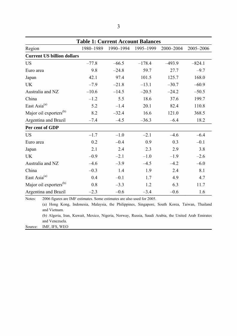
The past decade has seen sizeable changes in the current account positions of a number of regions around the world.1 From the start of the 1980s to the mid 1990s the US ran small current account deficits (fluctuating around 1½ per cent of GDP), as did some other developed English-speaking economies (Table 1). Developing economies in east Asia, Latin America and oil-producing regions also ran current account deficits during the early to mid 1990s. These deficits were offset by surpluses, primarily in Japan.

Since 1997 the US current account deficit has increased considerably, accompanied by increases in the deficits of some of the other English-speaking nations. Although Japan, and to a lesser extent the euro area, provided some offset to these deficits, a number of developing countries have become sizeable net exporters of savings. China has run a current account surplus since 1994, east Asia since 1998, the major oil exporters from 1999, and Argentina and Brazil (the two largest non-oil-exporting Latin American countries) since 2002. By the end of 2005 the combined surpluses of these developing countries accounted for around three-quarters of the US current account deficit. These movements took place during a period of rapidly appreciating asset prices in a number of developed countries and low long-term interest rates.

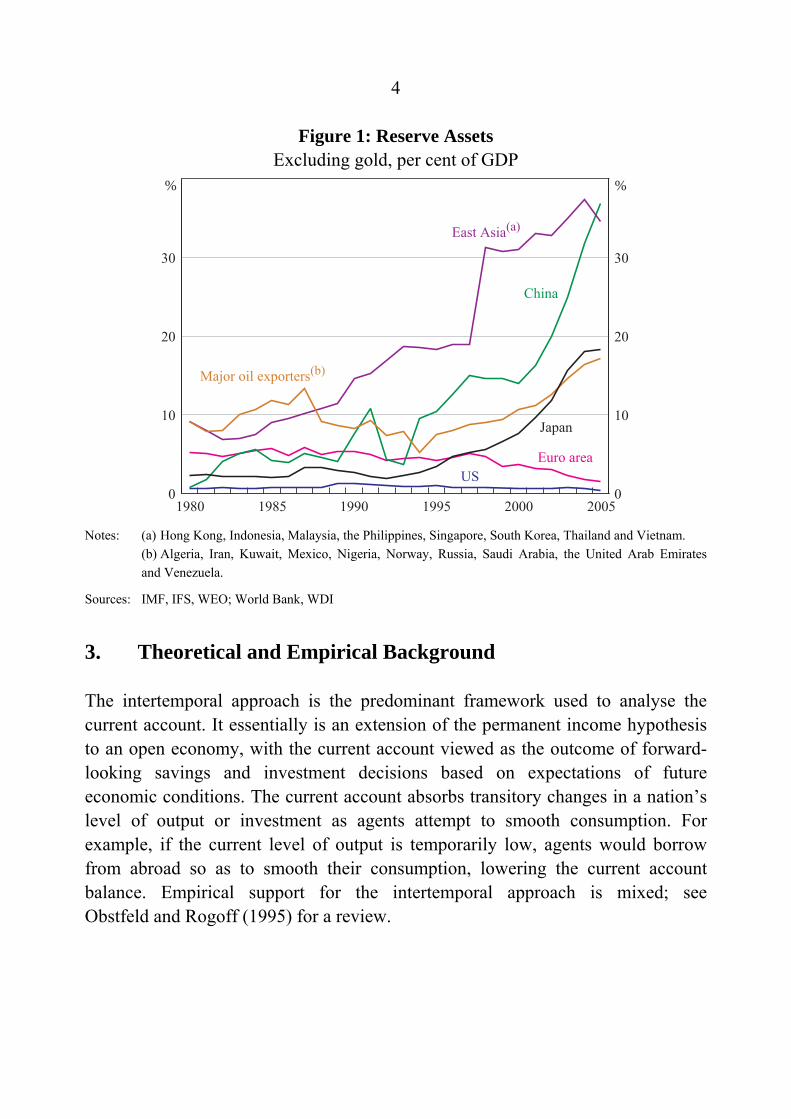
Another dimension of these global imbalances has been the accumulation of large stocks of foreign exchange reserves, primarily US dollars, by Asian central banks after the Asian crisis (Figure 1).

Escalating world oil and commodity prices may have also contributed to a change in the distribution of current account balances. Net natural resource exporters, many of which are developing nations, have benefited from a higher terms of trade. The trade balance of some of these countries has increased noticeably as a result. In line with this, it appears that only a small proportion of the increased oil revenues have been spent by oil-exporting nations.

1 For a comprehensive overview, see Orsmond (2005).

3

Table 1: Current Account Balances Region 1980–1989 1990–1994 1995–1999 2000–2004 2005–2006 Current US billion dollars US –77.8 –66.5 –178.4 –493.9 –824.1 Euro area 9.8 –24.8 59.7 27.7 –9.7 Japan 42.1 97.4 101.5 125.7 168.0 UK –7.9 –21.8 –13.1 –30.7 –60.9 Australia and NZ –10.6 –14.5 –20.5 –24.2 –50.5 China –1.2 5.5 18.6 37.6 199.7 East Asia(a) 5.2 –1.4 20.1 82.4 110.8 Major oil exporters(b) 8.2 –32.4 16.6 121.0 368.5 Argentina and Brazil –7.4 –4.5 –36.3 –6.4 18.2 Per cent of GDP US –1.7 –1.0 –2.1 –4.6 –6.4 Euro area 0.2 –0.4 0.9 0.3 –0.1 Japan 2.1 2.4 2.3 2.9 3.8 UK –0.9 –2.1 –1.0 –1.9 –2.6 Australia and NZ –4.6 –3.9 –4.5 –4.2 –6.0 China –0.3 1.4 1.9 2.4 8.1 East Asia(a) 0.4 –0.1 1.7 4.9 4.7 Major oil exporters(b) 0.8 –3.3 1.2 6.3 11.7 Argentina and Brazil –2.3 –0.6 –3.4 –0.6 1.6 Notes: 2006 figures are IMF estimates. Some estimates are also used for 2005. (a) Hong Kong, Indonesia, Malaysia, the Philippines, Singapore, South Korea, Taiwan, Thailand

and Vietnam. (b) Algeria, Iran, Kuwait, Mexico, Nigeria, Norway, Russia, Saudi Arabia, the United Arab Emirates

and Venezuela. Source: IMF, IFS, WEO

4

Figure 1: Reserve Assets Excluding gold, per cent of GDP

0

10

20

30

0

10

20

30

East Asia(a)

200520001995199019851980

China

Major oil exporters(b)

Euro areaUS

% %

Japan

Notes: (a) Hong Kong, Indonesia, Malaysia, the Philippines, Singapore, South Korea, Thailand and Vietnam. (b) Algeria, Iran, Kuwait, Mexico, Nigeria, Norway, Russia, Saudi Arabia, the United Arab Emirates

and Venezuela.

Sources: IMF, IFS, WEO; World Bank, WDI

3. Theoretical and Empirical Background

The intertemporal approach is the predominant framework used to analyse the current account. It essentially is an extension of the permanent income hypothesis to an open economy, with the current account viewed as the outcome of forward-looking savings and investment decisions based on expectations of future economic conditions. The current account absorbs transitory changes in a nation’s level of output or investment as agents attempt to smooth consumption. For example, if the current level of output is temporarily low, agents would borrow from abroad so as to smooth their consumption, lowering the current account balance. Empirical support for the intertemporal approach is mixed; see Obstfeld and Rogoff (1995) for a review.

5

This can be further extended to link a nation’s current account position to its stage of economic development. Countries that have a low level of development tend to have low capital-to-labour ratios and consequently the marginal product of capital is high. This implies that developing nations should tend to attract capital from developed countries where labour tends to be relatively scarce, resulting in developing countries running a current account deficit. As these nations reach a more advanced stage of development, they run current account surpluses to reduce their accumulated external liabilities and as the marginal product of capital falls. Empirical support for such effects has been limited (see for example Lucas 1990, Debelle and Faruqee 1996 and Chinn and Prasad 2003). One explanation for this, emphasised by Alfaro, Kalemil-Ozcan and Volosovych (2005), is that differences in institutional quality – such as the effectiveness of legal systems and the absence of corruption and political stability – bias capital flows towards developed nations.

Demographic variation can also be used to explain differences in current accounts across countries. If the implications of the life-cycle hypothesis are aggregated over individuals, a negative relationship should exist between aggregate domestic savings and the share of the non-working-age population. Masson, Bayoumi and Samiei (1995), Disney (1996) and Davis (2006) find evidence in support of this relationship.

The current account balance may react to the unanticipated component in a temporary positive (negative) terms of trade shock as consumers smooth their consumption by saving part of the income gain (borrowing to offset the income loss).2

The rapid increase in the US current account deficit over recent years has been the focus of a growing body of literature, some of which draws on the intertemporal framework. One view that has received considerable attention is the ‘global saving glut’ hypothesis of Bernanke (2005). Bernanke argues that financial crises cause capital flows to reverse, flowing from developing to industrialised countries. In

2 Kent and Cashin (2003) present evidence that the persistence of the terms of trade shock

influences its impact on the current account. In particular, with persistent shocks, savings will tend not to adjust much compared with investment, and consequently the terms of trade and the current account can move in opposite directions. However, in this paper we have not attempted to separate the predictable and unanticipated components of terms of trade movements, nor have we distinguished between transitory and persistent shocks.

6

particular, emerging market economies, especially in Asia, built up foreign exchange reserves to safeguard against potential future capital outflows and, to a lesser extent, as a result of promoting export-led growth (a point also discussed by Macfarlane 2005). In doing so, governments in these nations channelled domestic savings into international capital markets. Summers (2006) remarks that reserves in developing countries are at a level that is ‘far in excess of any previously enunciated criterion of reserves needed for financial protection’. Bernanke argues this excess saving placed downward pressure on real interest rates, stimulating borrowing, and consequently asset prices, in developed countries.

The importance of differences in the quality of financial markets and institutions in explaining developments in nations’ current accounts is emphasised by Caballero, Farhi and Gourinchas (2007). They argue that a change in the perception of the ability of domestic financial markets to provide sound financial instruments for savings results in increased funds flowing abroad. Such a re-evaluation could result from the onset of a financial crisis, with funds flowing to nations such as the US, which have more developed financial markets. In effect, Caballero et al are more explicit than Bernanke (2005) with regards to the transmission mechanism by which financial crises influence current accounts. They emphasise the role of a collapse in the supply of suitable financial assets domestically rather than growth in foreign reserves as the means by which domestic savings are driven abroad. In an earlier version of their paper, Caballero et al also argue that the stronger growth prospects of the US has caused these funds to flow to the US rather than to Europe, even though both economies have the ability to produce suitable financial assets. Such an outcome is also suggested by the intertemporal model of Engel and Rogers (2006).

An alternative model is provided by Dooley, Folkerts-Landau and Garber (2004a) (referred to as Bretton Woods II), who argue that developing countries have deliberately undervalued their exchange rates so as to promote growth in the traded-goods sector (and, for China, to absorb a large shift of rural workers to urban areas). It is also argued that developing countries are taking advantage of the higher quality of financial intermediation abroad by exporting their savings there as a form of collateral to obtain foreign direct investment to promote economic development (Dooley, Folkerts-Landau and Garber 2004b).

7

Recent empirical analysis has tended to support the notion that differences in the quality of financial markets and institutions across nations influence the size of the current account. Alfaro et al (2005) find that institutional quality is an important determinant of capital inflows, with a positive relationship existing between the two variables. Likewise, Gruber and Kamin (2007) find that improvements in the institutional quality of a nation’s markets lead to lower current account balances, as does stronger output growth. Similarly, Chinn and Ito (2007) find that a nation’s current account balance is likely to be lower, the higher is its level of legal development and the more open are its financial markets.

Gruber and Kamin (2007) find that financial crises have a significant effect on current account balances (when interacted with a term to capture trade openness). Hence, they argue that models using standard determinants of the current account should be augmented with variables representing financial crises. The authors postulate that financial crises encourage a current account surplus by restraining domestic demand and credit.

The increase in the US current account deficit has also been linked to the increase in the US fiscal deficit and the decline in the savings rate of US households. However, whether a decline in government or private savings actually leads to an increase in the current account deficit is ambiguous. For example, an increase in a nation’s fiscal deficit may decrease its current account balance if the private sector does not increase its saving to offset any rise in future liabilities due to the fiscal deficit (that is, if Ricardian equivalence does not apply). Simulations using a Federal Reserve Board macroeconomic model suggest that the increase in the budget deficit and the fall in private savings were only a minor factor contributing to the increase in the US current account deficit (Ferguson 2005). Similarly, Erceg, Guerrieri and Gust (2005) find that fiscal policy has a small effect on the trade balance.

8

4. Empirical Methodology and Data

Our dataset is an unbalanced panel of annual data for 34 countries over the period 1991–2005, accounting for nearly 90 per cent of global output in 2005. It includes all major economies together with a number of the major oil exporters and those countries directly affected by the Asian crisis.3 We choose to explain movements in the current account balance as a per cent of GDP. In contrast to previous studies, for example, those by Chinn and Ito (2007) and Gruber and Kamin (2007), which use five-year average data, our sample comprises annual data.4 We do this since annual data may allow us to better identify the impact of financial crises on the current account. In particular, it has the advantage of allowing for short crises whose impact would be muted by the use of five-year averages, and allows a profile for the impact of financial crises on current accounts to be derived.

The independent variables used in this study, which are outlined in greater detail below, can be grouped into two categories: (i) those variables which have traditionally been used to explain movements in the current account; and (ii) variables related to the newer theories that have arisen in response to the widening in the US current account deficit.

Since the sum of the current account balances of the nations in our sample equals zero (ignoring measurement error and assuming the net current account of the small countries excluded from our sample is balanced), a rise in one nation’s current account balance must be offset by a fall in the current account balances of other nations. Therefore, a uniform increase in an explanatory variable across all nations should have no effect on the aggregate current account balance of our sample. Accordingly, we have constructed our variables such that the aggregated predicted current account balance is unaffected by a common change in any explanatory variable. To do this, we typically express our explanatory variables as

3 The countries included in the data sample are Argentina, Australia, Belgium, Brazil, Canada,

China, France, Germany, Hong Kong, India, Indonesia, Iran, Italy, Japan, Kuwait, Malaysia, Mexico, the Netherlands, New Zealand, Nigeria, Norway, the Philippines, Russia, Singapore, South Africa, South Korea, Spain, Switzerland, Taiwan, Thailand, Turkey, the United Kingdom, the United States and Venezuela.

4 Chinn and Ito (2007) also estimate models based on annual data, however, these are not their primary focus.

9

deviations from GDP-weighted averages, consistent with the approach employed by Chinn and Ito (2007) and Gruber and Kamin (2007).5

The data are sourced primarily from cross-country databases, including the IMF’s International Financial Statistics (IFS) and the World Economic Outlook (WEO) and the World Bank’s World Development Indicators (WDI). For a comprehensive description of the data and its sources, see Appendix A.

4.1 Global Saving Glut and Financial Depth Variables

4.1.1 Financial crises

The global saving glut hypothesis attributes the shift of many developing nations to being net lenders to the ongoing impact of their financial crises. We identify financial crises as those episodes listed as: (i) systemic banking crises in Caprio and Klingebiel (2003); or (ii) a currency crisis lasting for at least 12 months by Kaminsky (2003).6 To limit endogeneity problems we exclude those financial crises attributed by Kaminsky to a widening of the current account deficit or sudden stops. Our definition of financial crises is consequently broader than that used by Gruber and Kamin (2007), who only consider systematic banking crises, although our results are not sensitive to using their narrower definition.7 We employ some flexibility in the dating of financial crises; we date those which occur late in a year as starting in the following year as they are unlikely to materially affect the annual data until then. A list of crises and their starting dates is presented in Appendix B.

5 The terms of trade is already a relative concept so deviations from GDP-weighted averages

were not calculated for this variable. 6 Crises that Caprio and Klingebiel (2003) date as at least a decade long are excluded (China,

Japan and Nigeria), however, their inclusion does not materially change the results. We also require crises in a particular nation to be more than 12 months apart.

7 Excluding non-banking crises increases the coefficients on the financial crisis dummies, but the results are not changed materially.

10

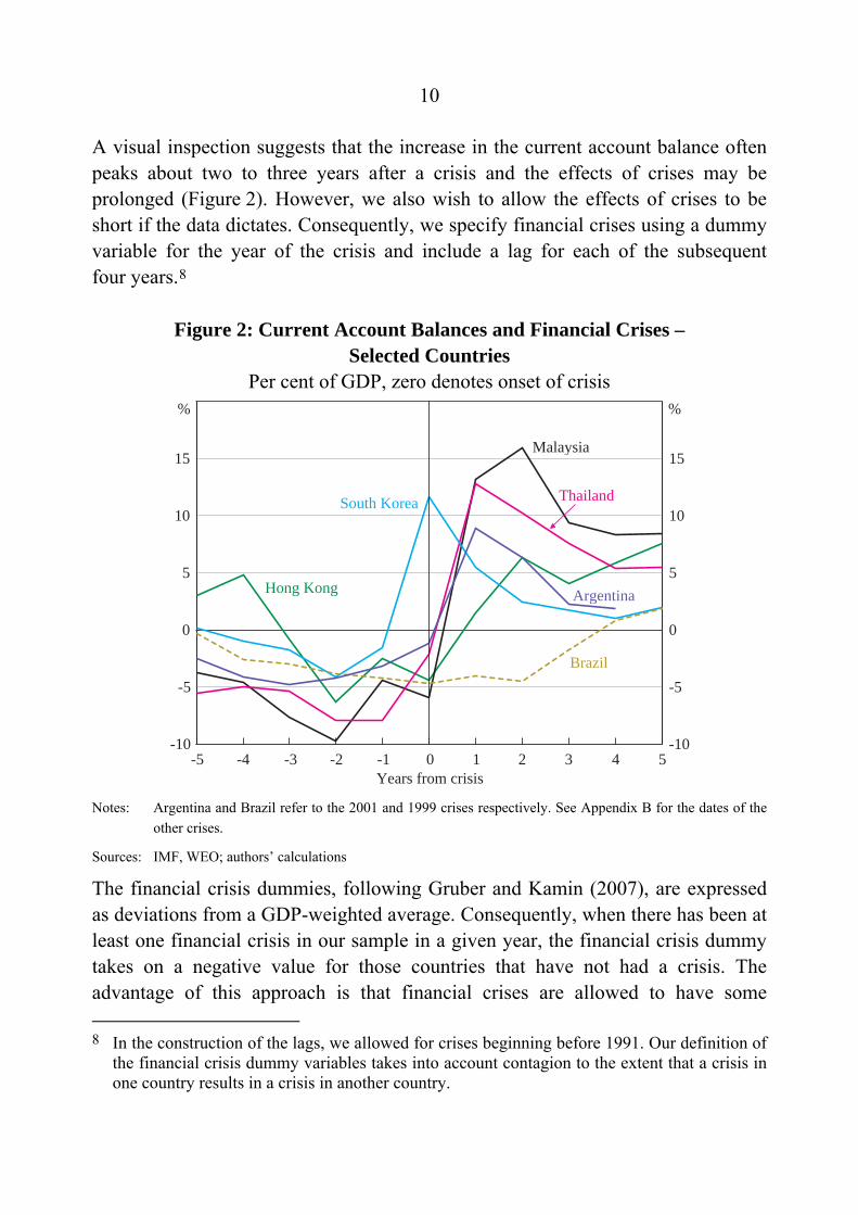
A visual inspection suggests that the increase in the current account balance often peaks about two to three years after a crisis and the effects of crises may be prolonged (Figure 2). However, we also wish to allow the effects of crises to be short if the data dictates. Consequently, we specify financial crises using a dummy variable for the year of the crisis and include a lag for each of the subsequent four years.8

Figure 2: Current Account Balances and Financial Crises – Selected Countries

Per cent of GDP, zero denotes onset of crisis

-10

-5

0

5

10

15

-10

-5

0

5

10

15

Years from crisis-5 3210-1-2-3-4 54

% %

Malaysia

ThailandSouth Korea

Hong Kong Argentina

Brazil

Notes: Argentina and Brazil refer to the 2001 and 1999 crises respectively. See Appendix B for the dates of the

other crises.

Sources: IMF, WEO; authors’ calculations

The financial crisis dummies, following Gruber and Kamin (2007), are expressed as deviations from a GDP-weighted average. Consequently, when there has been at least one financial crisis in our sample in a given year, the financial crisis dummy takes on a negative value for those countries that have not had a crisis. The advantage of this approach is that financial crises are allowed to have some 8 In the construction of the lags, we allowed for crises beginning before 1991. Our definition of

the financial crisis dummy variables takes into account contagion to the extent that a crisis in one country results in a crisis in another country.

11

(opposite) effect upon the current account balances of nations not in crisis. This is appropriate because the aggregate current account balance of the sample is still zero after each crisis.

4.1.2 Financial depth

In recent years private capital has flowed into the US and other developed countries. Caballero et al (2007) argue that this is partially because these countries are able to produce suitable financial instruments. We interpret this as meaning that financial markets in these countries are deeper and more liquid. We use annual stock market turnover as a proportion of share market capitalisation (the stock market turnover ratio) from Beck, Demirgüç-Kunt and Levine (2000) as a proxy for financial depth.9

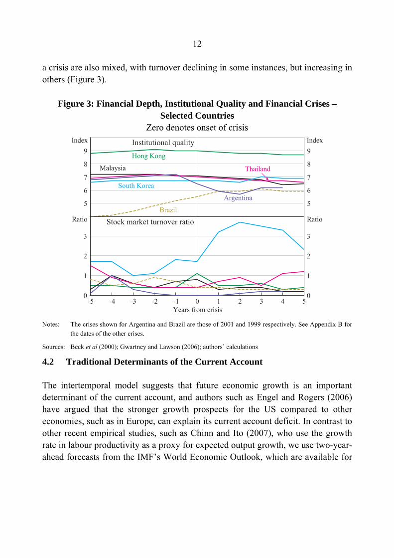
Liquidity is only one dimension of the ‘quality’ of financial assets; for example, the return on an investment also depends on the security of property rights. The quality of institutions in the US and a range of other developed countries may have been a factor contributing to their appeal as a destination for foreign private capital. We measure institutional quality using the Economic Freedom of the World index from Gwartney and Lawson (2006). This index is constructed using five equally weighted sub-indices, including measures of ‘legal structure and property rights’ and the ‘freedom to trade internationally’.10 These indices are bounded by zero and ten, with higher values denoting better institutional quality, and are based on both objective and subjective measures. Different measures of institutional quality are used by Chinn and Ito (2007) and Gruber and Kamin (2007). However, we choose the Economic Freedom of the World index because it is readily available and covers a greater range of countries over a longer time period. Movements in the index when financial crises occur are mixed; it does not tend to decline sharply, in part because it is not available at an annual frequency before 2000. Movements in stock market turnover following the onset of

9 In contrast, Chinn and Ito (2007) use the ratio of private credit to GDP as their proxy variable.

We obtain qualitatively similar results using their measure, in lieu of stock market turnover, over a longer sample (1980–2005).

10 The five sub-indices are: size of government expenditures, taxes and enterprises; legal structure and security of property rights; access to sound money; freedom to trade internationally; and regulation of credit, labour and business.

12

a crisis are also mixed, with turnover declining in some instances, but increasing in others (Figure 3).

Figure 3: Financial Depth, Institutional Quality and Financial Crises – Selected Countries

Zero denotes onset of crisis

5

6

7

8

9

5

6

7

8

9

Argentina

50

1

2

3

0

1

2

3

Institutional quality

Stock market turnover ratioBrazil

Malaysia

Hong Kong

Index Index

Thailand

South Korea

Ratio Ratio

-5 -4 -3 -2 -1 0 1 2 3 4Years from crisis

Notes: The crises shown for Argentina and Brazil are those of 2001 and 1999 respectively. See Appendix B for the dates of the other crises.

Sources: Beck et al (2000); Gwartney and Lawson (2006); authors’ calculations

4.2 Traditional Determinants of the Current Account

The intertemporal model suggests that future economic growth is an important determinant of the current account, and authors such as Engel and Rogers (2006) have argued that the stronger growth prospects for the US compared to other economies, such as in Europe, can explain its current account deficit. In contrast to other recent empirical studies, such as Chinn and Ito (2007), who use the growth rate in labour productivity as a proxy for expected output growth, we use two-year-ahead forecasts from the IMF’s World Economic Outlook, which are available for

13

a wide range of countries from 1991 onwards.11 These forecasts will include both expected cyclical fluctuations and growth in potential output. Caballero et al (2007) note that:

… it matters a great deal who is growing faster and who is growing slower than the US. If those that compete with the US in asset production (such as Europe) grow slower and those that demand assets (such as emerging Asia and oil producing economies) grow faster, then both factors play in the direction of generating capital flows towards the US. (p 16)

It is difficult to capture such effects in a model such as ours. However, in an attempt to do so we interact the growth forecasts with the three variables that cover various aspects of the perceived depth of a nation’s financial markets, namely, stock market depth, the quality of institutions and whether a financial crisis has occurred in the past five years.

To capture the effects of shifts in demographics and in the fiscal position, we include the dependency ratio (the ratio of the non-working-age population to the working-age population) and the fiscal balance as a per cent of GDP.12 Growth in the terms of trade (defined as the ratio of export prices to import prices) is included to control for, amongst other things, the effects of fluctuations in global oil and commodity prices on the current account balances of net natural resource exporting countries.

4.3 Estimation

We allow for unobserved time-invariant influences on each country’s current account balance by using a fixed-effects estimator. Chinn and Ito (2007) primarily pool data (one constant is estimated for all countries in the sample). The cost of using fixed effects relative to pooling is that we are unable to include variables that are time invariant in the regression. However, time-invariant factors are not a 11 This compares favourably to other potential sources, such as Consensus Forecasts. Over our

sample period, the WEO was published twice a year, in April or May and September or October. We use the April/May forecasts to maximise the forecast horizon. The cost of using these forecasts compared to labour productivity is that they are available for a much shorter time period. Nevertheless, the sample is constrained by the stock market turnover data.

12 The working-age population is defined as those aged between 15 and 64 years.

14

feature of the global saving glut hypothesis, nor Caballero et al’s (2007) hypotheses and, therefore, the ability to separately identify them is not of primary concern.

In summary, the regressions we estimate are of the form:

ititit

itititit

ititl

litl

itk

kitkit

itit

it

it

iti

it

it

sisongoingcrigrowthnsinstitutiogrowtheepnessfinancialdgrowth

ncefiscalbalagrowthdetermsoftra

nsinstitutiocrisiseepnessfinanciald

ratiodependencyGDPCAB

GDPCAB

GDPCAB

εβββ

βββ

βββ

βββη

+++

+++

+++

++++=

∑

∑

=−+

=−+

−

−

−

−

***

17

1615

1413

1

011

10

4

054

32

22

1

11

(1)

where: ηi is the fixed effect for country i; εit the error term; and βj are parameters.13 The model excluding lags of the current account balance is estimated by first differencing Equation (1) to remove the fixed effect and then using Ordinary Least Squares (OLS). When a lag of the dependent variable is included, the first lag of the current account balance will be correlated with the error term, and consequently we use two Stage Least Squares (2SLS), instrumenting the lagged dependent variable with a longer lag. This method is known as the Anderson-Hsiao estimator, after Anderson and Hsiao (1982).14 We chose this approach in lieu of using Generalized Method of Moments (GMM), following Arellano and Bond (1991), because our panel has a large time dimension but only a relatively small number of cross-sections. In this case, simulation evidence by Judson and

13 We assume that the slope parameters are the same across all countries. Relaxing this

assumption is complicated by the need to control for the global current account balance, but would be an interesting area of further research.

14 The estimation was conducted in Stata 9 using the xtserial and ivreg2 commands for OLS and 2SLS, which are due to Drukker (2003) and Baum, Schaffer and Stillman (2007).

15

Owen (1999) suggests that the simpler Anderson-Hsiao estimator performs comparatively well in terms of bias.15

5. Results

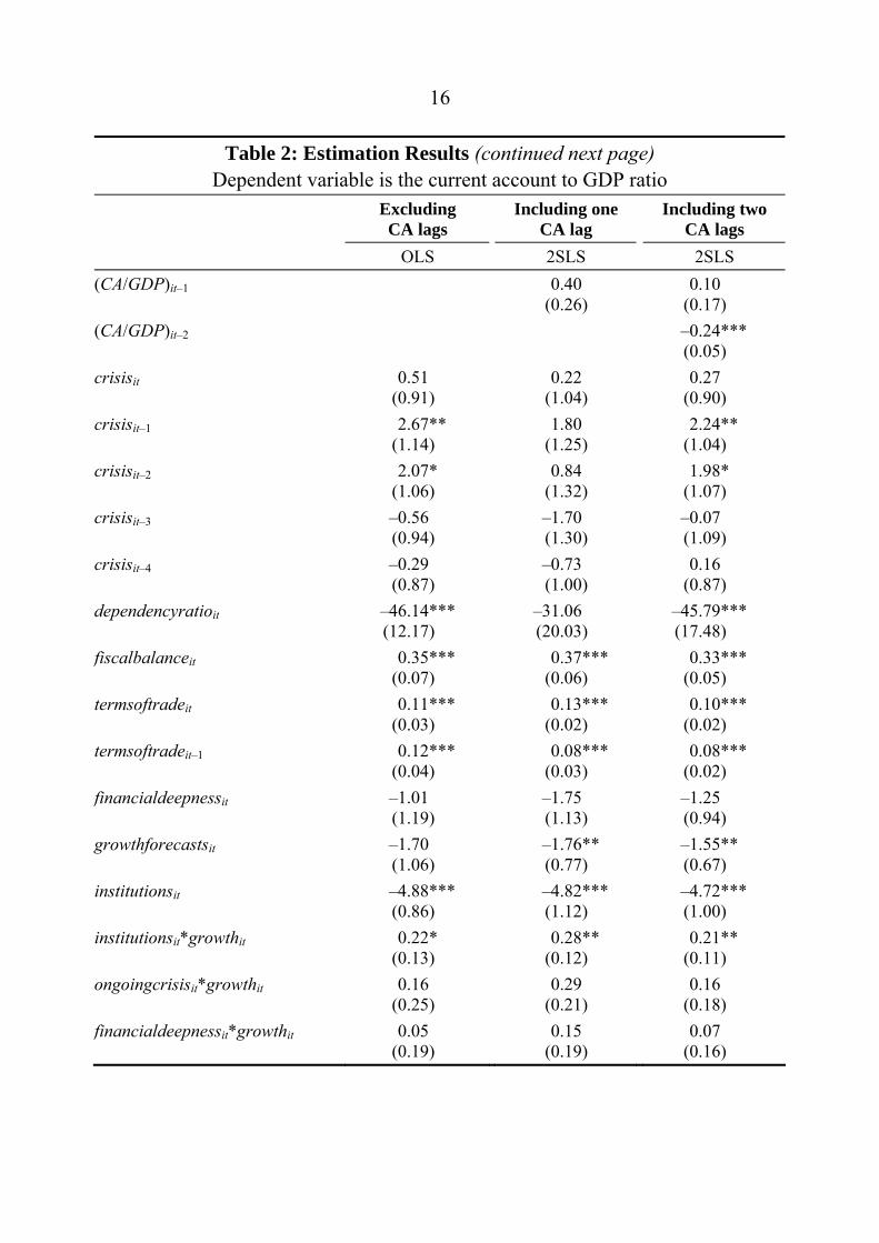
Table 2 presents the parameter estimates of our model with various lags of the dependent variable. If no lags are included the model has significant first-order autocorrelation; it is only when two lags are introduced that the regression displays no significant second-order autocorrelation.16 Gruber and Kamin (2007) note that the lag can be motivated by habit persistence and find it to be significant at the 10 per cent level despite using five-year average data. It may also reflect adjustment costs and uncertainty (Kent and Cashin 2003).

Focusing on the model with two lags of the dependent variable, we find that financial crises appear to have a significant and positive effect on the current account balance (as a per cent of GDP), which is around 2.2 percentage points higher in the year after the crisis.17 The effect of the crisis is short-lived – the crisis dummies for the third and fourth years after its onset are insignificant at the 10 per cent level. It is surprising that these effects do not last longer, given that after the Asian crisis, the building of ‘war chests’ of foreign reserves appears ongoing (see Figure 1). Nevertheless, the finding that financial crises do boost the current account balance is consistent with the global saving glut hypothesis, and contrasts with the findings of Gruber and Kamin (2007), whose models only found

15 See Roodman (2006) for a discussion of estimating dynamic panels using GMM. Another

alternative would be to use the approach of Kiviet (1995), which approximates the size of the bias and corrects for it, and is known as the Least Square Dummy Variable Corrected (LSDVC) estimator. Bruno (2005) generalises this estimator to unbalanced panels. However, it assumes that the explanatory variables are strictly exogenous, which in our case seems to be a strong assumption.

16 Second-order autocorrelation is problematic as it implies that the residuals in Equation (1) have first-order autocorrelation and that our instruments are inappropriate. The Arellano-Bond test for autocorrelation is implemented in Stata with the abar command (Roodman 2004).

17 In the discussion of the impact of a change in the explanatory variables, we assume that it does not alter the GDP-weighted average. This, obviously, is a poor approximation for a large country, such as the United States, for which any given change will have less impact (compared to a small country) as it will tend to lift the GDP-weighted average.

16

Table 2: Estimation Results (continued next page) Dependent variable is the current account to GDP ratio

Excluding CA lags

Including one CA lag

Including two CA lags

OLS 2SLS 2SLS (CA/GDP)it–1 0.40

(0.26) 0.10

(0.17) (CA/GDP)it–2 –0.24***

(0.05) crisisit 0.51

(0.91) 0.22

(1.04) 0.27

(0.90) crisisit–1 2.67**

(1.14) 1.80

(1.25) 2.24**

(1.04) crisisit–2 2.07*

(1.06) 0.84

(1.32) 1.98*

(1.07) crisisit–3 –0.56

(0.94) –1.70 (1.30)

–0.07 (1.09)

crisisit–4 –0.29 (0.87)

–0.73 (1.00)

0.16 (0.87)

dependencyratioit –46.14*** (12.17)

–31.06 (20.03)

–45.79*** (17.48)

fiscalbalanceit 0.35*** (0.07)

0.37*** (0.06)

0.33*** (0.05)

termsoftradeit 0.11*** (0.03)

0.13*** (0.02)

0.10*** (0.02)

termsoftradeit–1 0.12*** (0.04)

0.08*** (0.03)

0.08*** (0.02)

financialdeepnessit –1.01 (1.19)

–1.75 (1.13)

–1.25 (0.94)

growthforecastsit –1.70 (1.06)

–1.76** (0.77)

–1.55** (0.67)

institutionsit –4.88*** (0.86)

–4.82*** (1.12)

–4.72*** (1.00)

institutionsit*growthit 0.22* (0.13)

0.28** (0.12)

0.21** (0.11)

ongoingcrisisit*growthit 0.16 (0.25)

0.29 (0.21)

0.16 (0.18)

financialdeepnessit*growthit 0.05 (0.19)

0.15 (0.19)

0.07 (0.16)

17

Table 2: Estimation Results (continued) Dependent variable is the current account to GDP ratio

Excluding CA lags

Including one CA lag

Including two CA lags

OLS 2SLS 2SLS R2 0.38 0.21 0.40 Number of observations 444 444 443 Wooldridge test for autocorrelation (p-value)

0.00

Instruments (CA/GDP)it–2 ∆(CA/GDP)it–3 Arellano-Bond test (p-value) for second-order autocorrelation

0.00

0.76

Notes: Robust standard errors are shown in brackets. ***, ** and * denote significance at the 1, 5 and 10 per cent levels respectively. Fixed effects are not reported.

a positive relationship when the financial crisis dummy variable was interacted with a term to capture the openness of the economy.

Deeper financial markets appear to attract capital inflows and allow countries to run a lower current account balance than otherwise. This may reflect the greater ability of these nations to produce suitable financial assets (as suggested by Caballero et al 2007) or, more generally, they make a country a more attractive destination for foreign capital. However, the coefficient on stock market turnover (financial deepness), is not significantly different from zero at the 10 per cent level, which could, in part, reflect collinearity with the term that interacts this variable with the growth forecasts.18 A possible economic rationale for the insignificance of the stock market turnover coefficient is that the institutional quality variable – which is highly significant and has the expected negative sign – is capturing the ability to deliver suitable financial assets, as outlined in Caballero et al. If so, this would suggest that the onset of a financial crisis might not be associated with a sharp reversal in perceived financial depth, as the institutions variable tends not to vary much around a crisis (Figure 3).19 This may reflect both the infrequency with which the institutions variable is measured and the fact that, by construction, it

18 The magnitude of the coefficient remains broadly unchanged when the interaction term is

omitted, but the standard error decreases considerably. 19 On the flipside, the institutions measure may not capture improvements that might be

undertaken post-crisis in order to attract funds (including from the IMF).

18

places considerable weight upon objective (statistical) indicators of institutions and therefore it may not capture perceived institutional quality very well. It is possible that prior to the east Asian crisis, for example, investors were overly optimistic about the quality of prevailing institutions.

As we have not included a variable to explicitly capture the stage of development, one might have expected the institutions variable to do so. However, the negative coefficient for the institutions variable runs counter to the development hypothesis.

The fiscal balance is estimated to be an important determinant of the current account; a 1 percentage point reduction in the fiscal balance (relative to GDP) ratio is associated with an immediate 0.3 percentage point decrease in the current account balance (as a per cent of GDP). This estimate is approximately three times the value obtained by Gruber and Kamin (2007), but is within the range of estimates reported by Chinn and Ito (2007).20

Demographic factors are estimated to have a significant impact on a nation’s current account, with a 1 percentage point rise in the dependency ratio lowering the current account balance by around 0.5 percentage points of GDP. The direction of this effect is consistent with expectations, as the savings rate for dependents is likely to be less than that for the working-age population.

Bernanke (2005) argues that the increase in oil prices since the late 1990s was a factor contributing to nations in Africa and the Middle East shifting to be net lenders of capital. Our estimates broadly support this: growth in the terms of trade of 1 per cent in a year is estimated to increase a nation’s current account balance by around 0.2 percentage points of GDP by the end of the following year.

Better prospects for future growth appear to be associated with a significant decline in the current account balance. Ignoring the interaction terms, a 1 percentage point rise in the relative growth forecast is estimated to decrease the current account by around 1.6 percentage points of GDP. The interaction terms are generally insignificant. (These terms attempt to allow for the possibility that

20 Chinn and Ito raise the possibility that the fiscal balance is endogenous. When we instrument

the change in the fiscal balance with itself lagged two years, the coefficient drops to 0.14 and is insignificant.

19

growth may create demand for financial assets, but if domestic financial markets are unable to provide such assets then this would stimulate capital outflows.) The exception is the interaction between growth forecasts and the quality of institutions, which suggests, for example, that the marginal effect of an increase in the growth forecasts on the current account balance is more negative for nations with below-average institutions. We do not consider this strong evidence against the hypotheses of Caballero et al (2007), as it is difficult to capture the interactions between the supply and demand for financial assets in our model.

6. Implications for Regional Current Account Balances

In this section we examine the ability of the model to explain various elements of the global saving glut hypothesis, including the widening of the US current account deficit and the increased capital outflows from east Asia, China and the oil-producing nations.

The model estimates that the US current account deficit should have narrowed slightly from 1997 onwards, rather than the widening that actually occurred (Figure 4).21 This result was also obtained by Gruber and Kamin (2007), and while the model of Chinn and Ito (2007) predicts an increase in the current account deficit over this period, the estimated level is around 2 per cent of GDP, instead of the actual deficit of 5 per cent. Nevertheless, it is still instructive to look at the contributions of the various factors, which are shown in Figure 4.22 The large role attributed to the quality of institutions is immediately obvious; ignoring the interaction terms, as institutions in the US were above the GDP-weighted average for the entire sample, they contributed more than 3 percentage points to the current account deficit, although, interestingly, their contribution has decreased since the late 1990s. More generally, this supports Bernanke’s (2005) argument that, in order for developing countries to move to having net capital inflows, they should ‘… improve their investment climates by continuing to increase macroeconomic

21 To construct the estimate of the fixed effect, we take the parameters from our estimated

equation (which is the difference of Equation (1)) and apply them to Equation (1). The fixed effect for each country is then the average residual.

22 This figure was motivated by Figure 7 in Gruber and Kamin (2007).

20

stability, strengthen property rights, reduce corruption, and remove barriers to the free flow of financial capital’.

The estimated contribution of the widening of the fiscal deficit does not appear to have been the primary reason for the widening current account, despite being considerably larger than that in Gruber and Kamin (2007). Similarly, the influence of demographic factors is small, although this may in part reflect the inclusion of fixed effects.23 The impact of the increase in the growth forecasts since 2000 is reduced by the interaction with the institutions variable (included in ‘other’ in Figure 4).

Figure 4: Estimated Contribution to US Current Account Balance Per cent of GDP

Growth forecasts

%

2005200119971993

%

% %Other

Terms of trade

-2

0

2

-2

0

2Financial crisis

Fiscal balance Financial depth

Actual Fitted

Institutional quality

-8

-6

-4

-2

-8

-6

-4

-2

Sources: IMF, WEO; authors’ calculations

It is possible that the model does not capture the widening of the US current account deficit as it does not adequately ‘channel’ the impact of financial crises to the US.24 However, even if all of the increases in current account balances due to

23 In Figure 4, the demographic factors are in the ‘other’ aggregate, which also includes the

interaction terms and the lags of the current account, but excludes the fixed effect. 24 Recall that, in the model, the impact of financial crises are ‘channelled’ to the non-crisis

countries as the dummy variables enter as deviations from the GDP-weighted average.

21

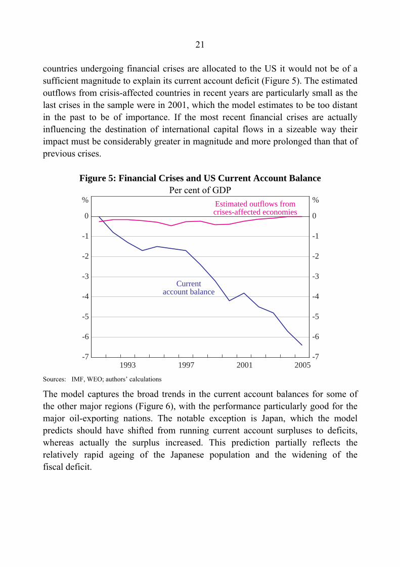
countries undergoing financial crises are allocated to the US it would not be of a sufficient magnitude to explain its current account deficit (Figure 5). The estimated outflows from crisis-affected countries in recent years are particularly small as the last crises in the sample were in 2001, which the model estimates to be too distant in the past to be of importance. If the most recent financial crises are actually influencing the destination of international capital flows in a sizeable way their impact must be considerably greater in magnitude and more prolonged than that of previous crises.

Figure 5: Financial Crises and US Current Account Balance Per cent of GDP

-7

-6

-5

-4

-3

-2

-1

0

-7

-6

-5

-4

-3

-2

-1

0

2005

Currentaccount balance

%

200119971993

Estimated outflows fromcrises-affected economies

%

Sources: IMF, WEO; authors’ calculations

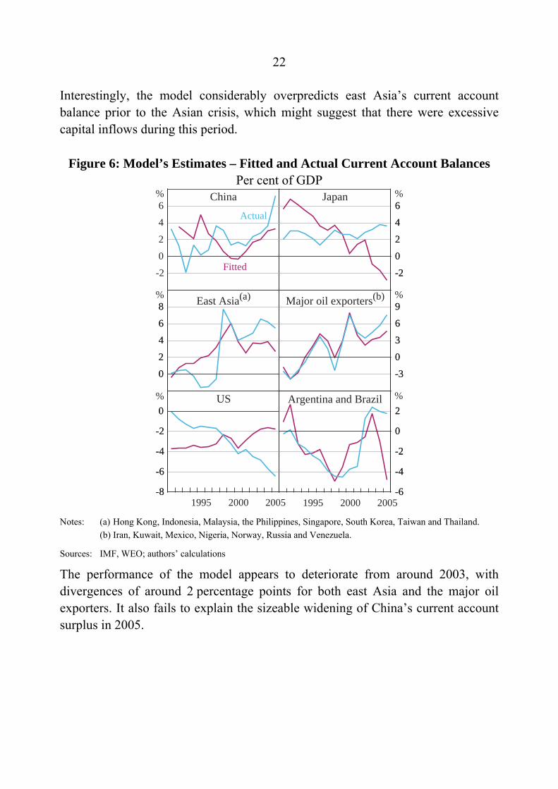
The model captures the broad trends in the current account balances for some of the other major regions (Figure 6), with the performance particularly good for the major oil-exporting nations. The notable exception is Japan, which the model predicts should have shifted from running current account surpluses to deficits, whereas actually the surplus increased. This prediction partially reflects the relatively rapid ageing of the Japanese population and the widening of the fiscal deficit.

22

Interestingly, the model considerably overpredicts east Asia’s current account balance prior to the Asian crisis, which might suggest that there were excessive capital inflows during this period.

Figure 6: Model’s Estimates – Fitted and Actual Current Account Balances Per cent of GDP

-8

-6

-4

-2

0

-8

-6

-4

-2

0

0

2

4

6

8

0

2

4

6

8

-3

0

3

6

9

-3

0

3

6

9

Fitted

China

-2

0

2

4

6

-2

0

2

4

6

-2

0

2

4

6Japan

East Asia(a) Major oil exporters(b)

US

Actual

%%

%%

%

200520001995-6

-4

-2

0

2

-6

-4

-2

0

2Argentina and Brazil %

200520001995 Notes: (a) Hong Kong, Indonesia, Malaysia, the Philippines, Singapore, South Korea, Taiwan and Thailand. (b) Iran, Kuwait, Mexico, Nigeria, Norway, Russia and Venezuela.

Sources: IMF, WEO; authors’ calculations

The performance of the model appears to deteriorate from around 2003, with divergences of around 2 percentage points for both east Asia and the major oil exporters. It also fails to explain the sizeable widening of China’s current account surplus in 2005.

23

7. Sensitivity Analysis

7.1 The Exchange Rate

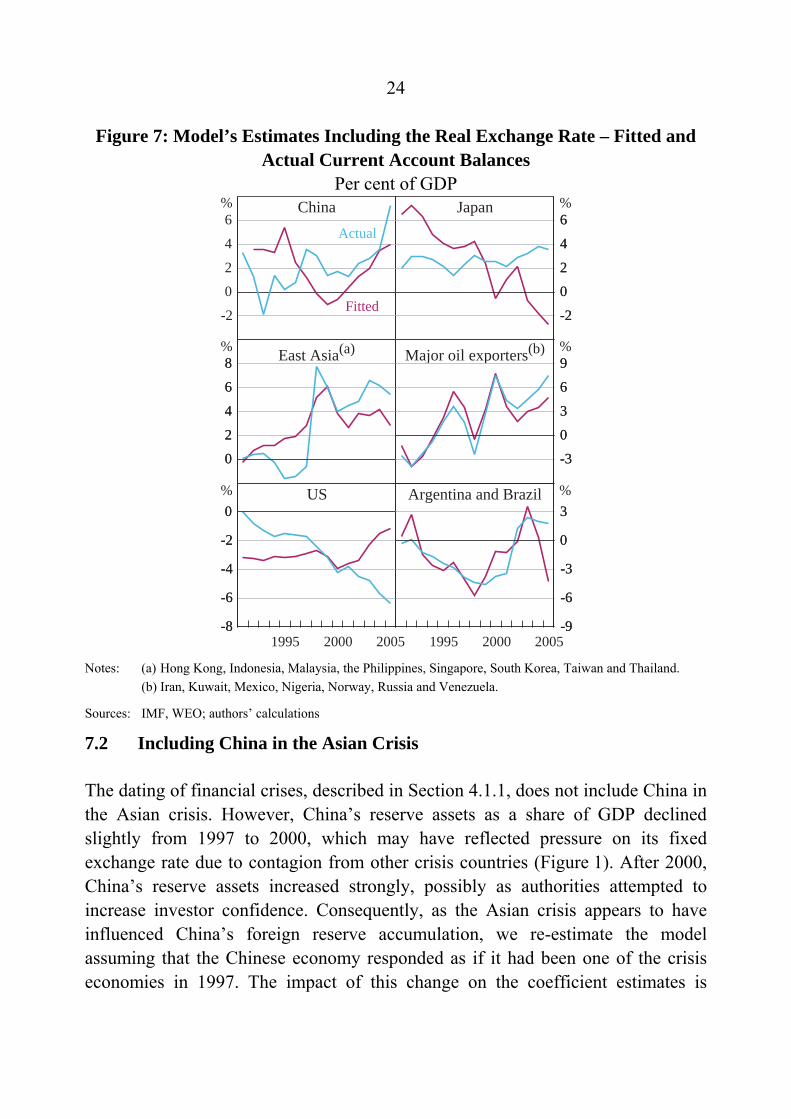
Dooley et al (2004a) argue that some countries (such as China) have undervalued their exchange rate in order to promote growth in the traded sector, and view the substantial increases in foreign exchange reserves as a consequence of this policy.25 This has not been accounted for explicitly in our model, although the financial crisis dummy variables may partially capture the increase in reserves. We experimented with adding the real exchange rate to the model as a deviation from a statistical trend estimate, and included one lag (see Appendix C for the model results).26 The performance of the model appears to improve for several regions for particular periods (compare Figures 6 and 7) – such as the major oil exporters during 1996, China from 2003 onwards, and the US from 1999–2001. However, the overall improvement to the fit of the model from including the real exchange rate is small.27

25 Bergin and Sheffrin (2000) extend the intertemporal model to include the real exchange rate. 26 We use a Hodrick-Prescott (1997) filter to isolate the cyclical component. We set the

smoothing parameter to 400, which yields a very smooth trend estimate. Similar results were obtained with lower values.

27 The real exchange rate may be endogenous. If we instrument it with longer lags (which may be weak instruments), the fitted values display the same broad trends as in Figure 7, but are more volatile.

24

Figure 7: Model’s Estimates Including the Real Exchange Rate – Fitted and Actual Current Account Balances

Per cent of GDP

-8

-6

-4

-2

0

-8

-6

-4

-2

0

0

2

4

6

8

0

2

4

6

8

-3

0

3

6

9

-3

0

3

6

9

Fitted

China

-2

0

2

4

6

-2

0

2

4

6

-2

0

2

4

6Japan

US

Actual

%%

%%

%

200520001995-9

-6

-3

0

3

-9

-6

-3

0

3Argentina and Brazil %

200520001995

East Asia(a) Major oil exporters(b)

Notes: (a) Hong Kong, Indonesia, Malaysia, the Philippines, Singapore, South Korea, Taiwan and Thailand. (b) Iran, Kuwait, Mexico, Nigeria, Norway, Russia and Venezuela.

Sources: IMF, WEO; authors’ calculations

7.2 Including China in the Asian Crisis

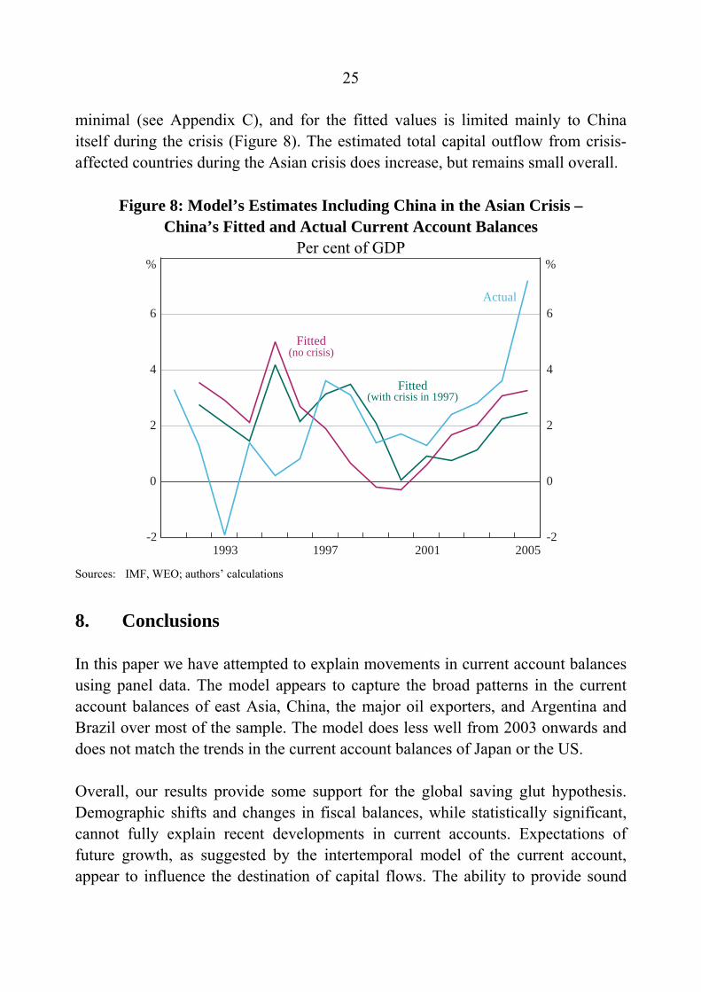
The dating of financial crises, described in Section 4.1.1, does not include China in the Asian crisis. However, China’s reserve assets as a share of GDP declined slightly from 1997 to 2000, which may have reflected pressure on its fixed exchange rate due to contagion from other crisis countries (Figure 1). After 2000, China’s reserve assets increased strongly, possibly as authorities attempted to increase investor confidence. Consequently, as the Asian crisis appears to have influenced China’s foreign reserve accumulation, we re-estimate the model assuming that the Chinese economy responded as if it had been one of the crisis economies in 1997. The impact of this change on the coefficient estimates is

25

minimal (see Appendix C), and for the fitted values is limited mainly to China itself during the crisis (Figure 8). The estimated total capital outflow from crisis-affected countries during the Asian crisis does increase, but remains small overall.

Figure 8: Model’s Estimates Including China in the Asian Crisis – China’s Fitted and Actual Current Account Balances

Per cent of GDP

-2

0

2

4

6

-2

0

2

4

6

(no crisis)

Actual

Fitted

% %

Fitted

(with crisis in 1997)

2005200119971993 Sources: IMF, WEO; authors’ calculations

8. Conclusions

In this paper we have attempted to explain movements in current account balances using panel data. The model appears to capture the broad patterns in the current account balances of east Asia, China, the major oil exporters, and Argentina and Brazil over most of the sample. The model does less well from 2003 onwards and does not match the trends in the current account balances of Japan or the US.

Overall, our results provide some support for the global saving glut hypothesis. Demographic shifts and changes in fiscal balances, while statistically significant, cannot fully explain recent developments in current accounts. Expectations of future growth, as suggested by the intertemporal model of the current account, appear to influence the destination of capital flows. The ability to provide sound

26

financial instruments, as emphasised by Caballero et al (2007), may be important, as the quality of institutions was found to have a large effect. In order to fully evaluate the interaction between supply and demand of financial assets, which Caballero et al emphasise, a more structural model is probably required. Additionally, some of the determinants of international capital flows – such as the perceived quality of financial markets, institutions, or investor sentiment – are inherently difficult to measure. Finally, financial crises do appear to increase net capital outflows from crisis regions for a number of years, although the estimated magnitude of these effects is insufficient to fully explain the pattern of recent international capital flows.

27

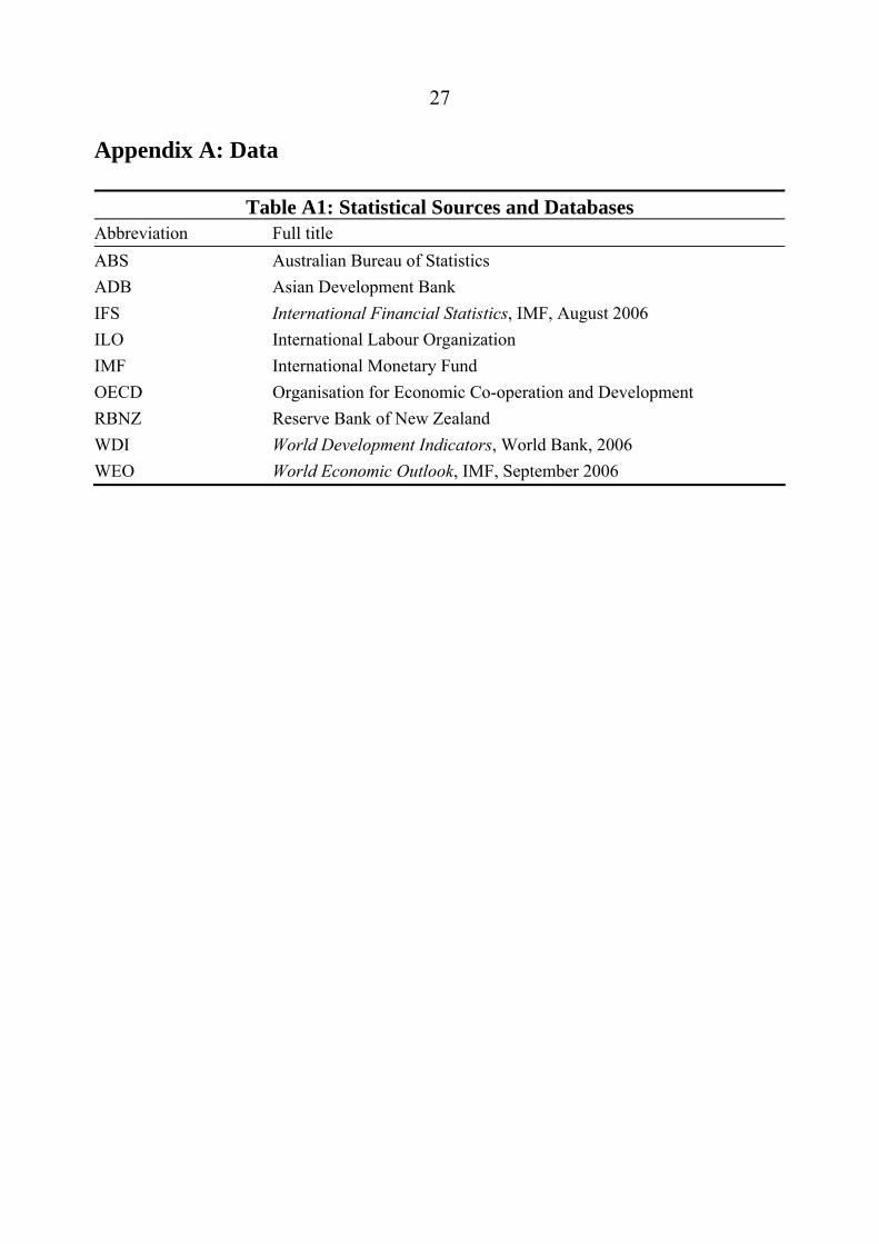
Appendix A: Data

Table A1: Statistical Sources and Databases Abbreviation Full title ABS Australian Bureau of Statistics ADB Asian Development Bank IFS International Financial Statistics, IMF, August 2006 ILO International Labour Organization IMF International Monetary Fund OECD Organisation for Economic Co-operation and Development RBNZ Reserve Bank of New Zealand WDI World Development Indicators, World Bank, 2006 WEO World Economic Outlook, IMF, September 2006

28

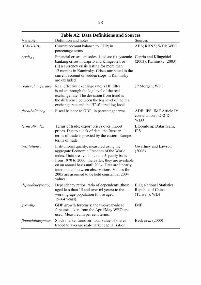
Table A2: Data Definitions and Sources Variable Definition and notes Sources (CA/GDP)it Current account balance to GDP; in

percentage terms. ABS; RBNZ; WDI; WEO

crisisit-k Financial crises; episodes listed as: (i) systemic banking crises in Caprio and Klingebiel; or (ii) a currency crisis lasting for more than 12 months in Kaminsky. Crises attributed to the current account or sudden stops in Kaminsky are excluded.

Caprio and Klingebiel (2003); Kaminsky (2003)

realexchangerateit Real effective exchange rate; a HP filter is taken through the log level of the real exchange rate. The deviation from trend is the difference between the log level of the real exchange rate and the HP-filtered log level.

JP Morgan; WDI

fiscalbalanceit Fiscal balance to GDP; in percentage terms. ADB; IFS; IMF Article IV consultations; OECD; WEO

termsoftradeit Terms of trade; export prices over import prices. Due to a lack of data, the Russian terms of trade is proxied by the eastern Europe terms of trade.

Bloomberg; Datastream; IFS

institutionsit Institutional quality; measured using the aggregate Economic Freedom of the World index. Data are available on a 5-yearly basis from 1970 to 2000; thereafter, they are available on an annual basis until 2004. Data are linearly interpolated between observations. Values for 2005 are assumed to be held constant at 2004 values.

Gwartney and Lawson (2006)

dependencyratioit Dependency ratios; ratio of dependents (those aged less than 15 and over 64 years) to the working-age population (those aged 15–64 years).

ILO; National Statistics Republic of China (Taiwan); WDI

growthit GDP growth forecasts; the two-year-ahead forecasts taken from the April/May WEO are used. Measured in per cent terms.

IMF

financialdeepnessit Stock market turnover; total value of shares traded to average real-market capitalisation.

Beck et al (2000)

29

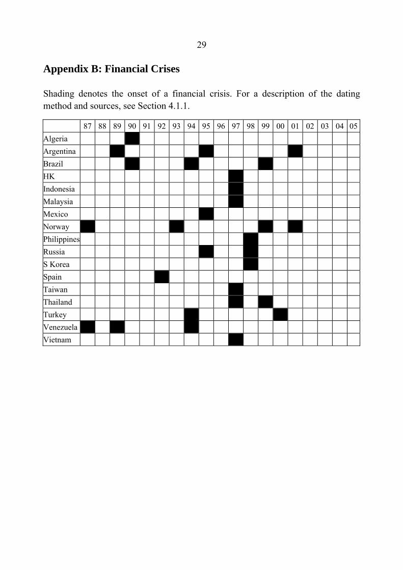
Appendix B: Financial Crises

Shading denotes the onset of a financial crisis. For a description of the dating method and sources, see Section 4.1.1.

87 88 89 90 91 92 93 94 95 96 97 98 99 00 01 02 03 04 05Algeria Argentina Brazil HK Indonesia Malaysia Mexico Norway Philippines Russia S Korea Spain Taiwan Thailand Turkey Venezuela Vietnam

30

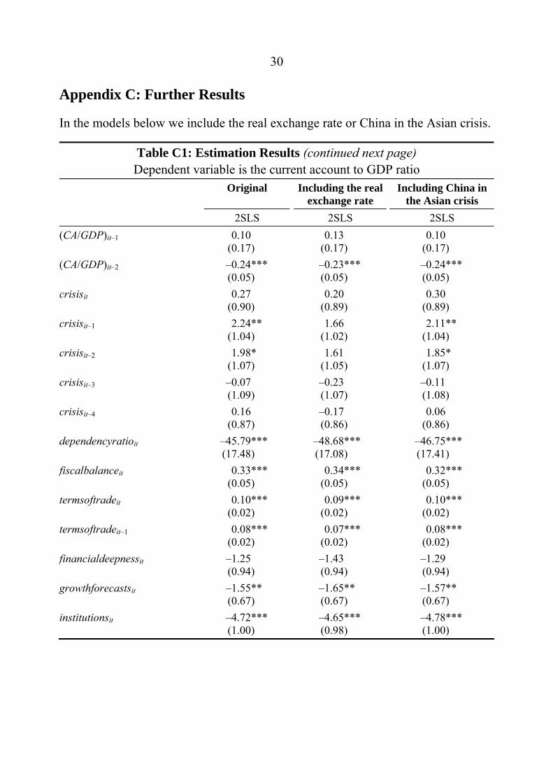
Appendix C: Further Results

In the models below we include the real exchange rate or China in the Asian crisis.

Table C1: Estimation Results (continued next page) Dependent variable is the current account to GDP ratio

Original Including the real exchange rate

Including China in the Asian crisis

2SLS 2SLS 2SLS (CA/GDP)it–1 0.10

(0.17) 0.13

(0.17) 0.10

(0.17) (CA/GDP)it–2 –0.24***

(0.05) –0.23*** (0.05)

–0.24*** (0.05)

crisisit 0.27 (0.90)

0.20 (0.89)

0.30 (0.89)

crisisit–1 2.24** (1.04)

1.66 (1.02)

2.11** (1.04)

crisisit–2 1.98* (1.07)

1.61 (1.05)

1.85* (1.07)

crisisit–3 –0.07 (1.09)

–0.23 (1.07)

–0.11 (1.08)

crisisit–4 0.16 (0.87)

–0.17 (0.86)

0.06 (0.86)

dependencyratioit –45.79*** (17.48)

–48.68*** (17.08)

–46.75*** (17.41)

fiscalbalanceit 0.33*** (0.05)

0.34*** (0.05)

0.32*** (0.05)

termsoftradeit 0.10*** (0.02)

0.09*** (0.02)

0.10*** (0.02)

termsoftradeit–1 0.08*** (0.02)

0.07*** (0.02)

0.08*** (0.02)

financialdeepnessit –1.25 (0.94)

–1.43 (0.94)

–1.29 (0.94)

growthforecastsit –1.55** (0.67)

–1.65** (0.67)

–1.57** (0.67)

institutionsit –4.72*** (1.00)

–4.65*** (0.98)

–4.78*** (1.00)

31

Table C1: Estimation Results (continued) Dependent variable is the current account to GDP ratio

Original Including the real exchange rate

Including China in the Asian crisis

2SLS 2SLS 2SLS institutionsit*growthit 0.21**

(0.11) 0.23**

(0.11) 0.21**

(0.11) ongoingcrisisit*growthit 0.16

(0.18) 0.16

(0.18) 0.19

(0.17) financialdeepnessit*growthit 0.07

(0.16) 0.10

(0.16) 0.09

(0.16) realexchangerateit –0.007

(0.01)

realexchangerateit–1 –0.07*** (0.01)

R2 0.40 0.42 0.40 Number of observations 443 443 443 Instruments ∆(CA/GDP)it–3 ∆(CA/GDP)it–3 ∆(CA/GDP)it–3 Arellano-Bond test (p-value) for second-order autocorrelation

0.76

0.27

0.76

Notes: Robust standard errors are shown in brackets. ***, ** and * denote significance at the 1, 5 and 10 per cent levels respectively. Fixed effects are not reported.

32

References

Alfaro L, S Kalemil-Ozcan and V Volosovych (2005), ‘Capital Flows in a Globalized World: The Role of Policies and Institutions’, NBER Working Paper No 11696.

Anderson TW and C Hsiao (1982), ‘Formulation and Estimation of Dynamic Models Using Panel Data’, Journal of Econometrics, 18(1), pp 47–82.

Arellano M and S Bond (1991), ‘Some Tests of Specification for Panel Data: Monte Carlo Evidence and an Application to Employment Equations’, Review of Economic Studies, 58(2), pp 277–297.

Baum CF, ME Schaffer and S Stillman (2007) database, ‘IVREG2: Stata Module for Extended Instrumental Variables/2SLS and GMM Estimation, available at <http://econpapers.repec.org/software/bocbocode/s425401.htm>.

Beck T, A Demirgüç-Kunt and R Levine (2000), ‘A New Database on the Structure and Development of the Financial Sector’, The World Bank Economic Review, 14(3), pp 597–605. An updated database is available at <http://econ.worldbank.org/WBSITE/EXTERNAL/EXTDEC/EXTRESEARCH/0,,contentMDK:20696167~pagePK:64214825~piPK:64214943~theSitePK:469382,00.html>.

Bergin PR and SM Sheffrin (2000), ‘Interest Rates, Exchange Rates and Present Value Models of the Current Account’, The Economic Journal, 110(463), pp 535–558.

Bernanke B (2005), ‘The Global Saving Glut and the U.S. Current Account Deficit’, Remarks at the Homer Jones Lecture, St. Louis, 14 April.

Bruno GSF (2005), ‘Approximating the Bias of the LSDV Estimator for Dynamic Unbalanced Panel Data Models’, Economics Letters, 87(3), pp 361–366.

33

Caballero RJ, E Farhi and PO Gourinchas (2007), ‘An Equilibrium Model of “Global Imbalances” and Low Interest Rates’, available at <http://econ-www.mit. edu/faculty/ download_pdf.php?id=1234>.

Caprio G and D Klingebiel (2003) database, ‘Episodes of Systemic and Borderline Financial Crisis’, available at <http://go.worldbank.org/ 5DYGICS7B0>.

Chinn MD and H Ito (2007), ‘Current Account Balances, Financial Development and Institutions: Assaying the World “Savings Glut”’, Journal of International Money and Finance, 26(4), pp 546–569.

Chinn MD and ES Prasad (2003), ‘Medium-term Determinants of Current Accounts in Industrial and Developing Countries: An Empirical Exploration’, Journal of International Economics, 59(1), pp 47–76.

Davis EP (2006), ‘How Will Ageing Affect the Structure of Financial Markets?’, in C Kent, A Park and D Rees (eds), Demography and Financial Markets, Proceedings of a Conference, Reserve Bank of Australia, Sydney, pp 266–295.

Debelle G and H Faruqee (1996), ‘What Determines the Current Account? A Cross-Sectional and Panel Approach’, IMF Working Paper No 96/58.

Disney R (1996), Can we Afford to Grow Older?, MIT Press, Cambridge.

Dooley MP, D Folkerts-Landau and PM Garber (2004a), ‘Direct Investment, Rising Real Wages and the Absorption of Excess Labor in the Periphery’, NBER Working Paper No 10626.

Dooley MP, D Folkerts-Landau and PM Garber (2004b), ‘The US Current Account Deficit and Economic Development: Collateral for a Total Return Swap’, NBER Working Paper No 10727.

Drukker DM (2003), ‘Testing for Serial Correlation in Linear Panel-Data Models’, The Stata Journal, 3(2), pp 168–177.

34

Engel C and JH Rogers (2006), ‘The U.S. Current Account Deficit and the Expected Share of World Output’, Journal of Monetary Economics, 53(5), pp 1063–1093

Erceg CJ, L Guerrieri and C Gust (2005), ‘Expansionary Fiscal Shocks and the US Trade Deficit’, International Finance, 8(3), pp 363–397.

Ferguson RW (2005), ‘US Current Account Deficits: Causes and Consequences’, Speech at the Carolina Economics Club of the University of North Carolina at Chapel Hill, 20 April.

Gruber JW and SB Kamin (2007), ‘Explaining the Global Pattern of Current Account Imbalances’, Journal of International Money and Finance, 26(4), pp 500–522.

Gwartney JD and RA Lawson (2006), Economic Freedom of the World: 2006 Annual Report, The Fraser Institute, Vancouver.

Hodrick RJ and EC Prescott (1997), ‘Postwar U.S. Business Cycles: An Empirical Investigation’, Journal of Money, Credit and Banking, 29(1), pp 1–16.

Judson RA and AL Owen (1999), ‘Estimating Dynamic Panel Data Models: A Guide for Macroeconomists’, Economics Letters, 65(1), pp 9–15.

Kaminsky GL (2003), ‘Varieties of Currency Crises’, NBER Working Paper No 10193.

Kent C and P Cashin (2003), ‘The Response of the Current Account to Terms of Trade Shocks: Persistence Matters’, IMF Working Paper No 03/143.

Kiviet JF (1995), ‘On Bias, Inconsistency, and Efficiency of Various Estimators in Dynamic Panel Data Models’, Journal of Econometrics, 68(1), pp 53–78.

Lucas RE Jr (1990), ‘Why Doesn’t Capital Flow from Rich to Poor Countries?’, The American Economic Review, 80(2), pp 92–96.

35

Macfarlane IJ (2005), ‘Payments Imbalances’, presentation to the Chinese Academy of Social Sciences, Beijing, 12 May.

Masson PR, TA Bayoumi and H Samiei (1995), ‘International Evidence on the Determinants of Private Savings’, IMF Working Paper No 95/51.

Obstfeld M and K Rogoff (1995), ‘The Intertemporal Approach to the Current Account’, in GM Grossman and K Rogoff (eds), Handbook of International Economics: Volume 3, North-Holland, Amsterdam, pp 1731–1799.

Orsmond D (2005), ‘Recent Trends in World Saving and Investment Patterns’, RBA Bulletin, October, pp 28–36.

Roodman D (2004), ‘ABAR: Module to Perform Arellano-Bond Test for Autocorrelation’, available at <http://ideas.repec.org/c/boc/bocode/s437501.html>.

Roodman D (2006), ‘How to Do xtabond2: An Introduction to “Difference” and “System” GMM in Stata’, Center for Global Development Working Paper No 103.

Summers LH (2006), ‘Reflections on Global Account Imbalances and Emerging Markets Reserve Accumulation’, LK Jha Memorial Lecture, Reserve Bank of India, Mumbai, 24 March.