research discussion paper - reserve bank of australia · research discussion paper the life of...

Research Discussion Paper

The Life of Australian Banknotes

Alexandra Rush

RDP 2015-10

The contents of this publication shall not be reproduced, sold or distributed without the prior consent of the Reserve Bank of Australia and, where applicable, the prior consent of the external source concerned. Requests for consent should be sent to the Head of Information Department at the email address shown above.

ISSN 1448-5109 (Online)

The Discussion Paper series is intended to make the results of the current economic research within the Reserve Bank available to other economists. Its aim is to present preliminary results of research so as to encourage discussion and comment. Views expressed in this paper are those of the authors and not necessarily those of the Reserve Bank. Use of any results from this paper should clearly attribute the work to the authors and not to the Reserve Bank of Australia.

Enquiries:

Phone: +61 2 9551 9830 Facsimile: +61 2 9551 8033 Email: [email protected] Website: http://www.rba.gov.au


Alexandra Rush

Research Discussion Paper 2015-10

August 2015

Note Issue Department Reserve Bank of Australia

I thank Michele Bullock, Christopher Kent, Michael Andersen, John Simon, Thomas Rohling, Peter Tulip, James Hansen and Matthew Read for valuable comments and contributions. The views expressed in this paper are those of the author and do not necessarily reflect the views of the Reserve Bank of Australia. The author is solely responsible for any errors.

Author: [email protected]

Media Office: [email protected]

i

Abstract

Understanding the life of banknotes is important to a currency issuer’s forward planning. Without accurate predictions of banknote life, there is a risk of incurring the economic costs of overproducing and storing excess banknotes or conversely, in an extreme case, of not being able to meet the public’s demand. The life of a banknote, however, is not directly observed and must be estimated – a process complicated by the manner in which banknotes are issued and circulated. Often currency issuers use simple turnover formulas to estimate the mean or median life of banknotes; however, such measures tend to be particularly volatile over time as they cannot take into account shocks to currency demand, or changes to currency issuer policies that affect distribution arrangements or the quality of circulating banknotes.

This paper proposes an alternative way of studying banknote life by estimating survival models, which are commonly used in studying life expectancies in medicine or the duration of events in economics. These models can produce estimates of central tendency that are much less volatile over time and provide information on the probability that banknotes survive over time. The models’ predictions of banknote survival are intuitive and the results are consistent with samples of circulating and unfit banknotes.

JEL Classification Numbers: C41, E42, E58 Keywords: banknotes, banknote life, currency, turnover, survival analysis,

nonlinear regression

ii

Table of Contents

1. Introduction 1

2. Background 2

2.1 The Life of a Banknote 2

2.2 Parallels in Other Literature Areas 4

2.3 Characterising the Deterioration of Banknotes 5

2.4 The Expected Shape of Hazard Functions 6

3. Traditional Steady-state or Turnover Method 7

4. ‘Feige’ Steady-state Method 11

5. Limitations of the Steady-state Methods 14

5.1 Demand Shocks 14

5.2 Banknote Quality Programs 15

5.3 New Banknote Series 15

5.4 Cash Management 16

6. Survival Modelling 16

6.1 Model Specification 16

6.2 Survival Model Results 22

6.3 Banknote Life Estimates 25

7. Back-testing the Models 27

7.1 Sampling Unfit Banknotes 27

7.2 Sampling Banknotes in Circulation 29

8. Conclusion 31

Appendix A: Deriving the Feige Steady-state Equation 33

iii

Appendix B: Survival Model Functions 35

Appendix C: Other Survival Model Specifications 38

References 39


Alexandra Rush

1. Introduction

Knowledge of the life of a banknote is important to managing an issuer’s banknote production, processing, distribution and storage requirements. To make these policy decisions, currency issuers need an understanding of how long banknotes can remain in circulation before they are no longer fit for purpose and need to be replaced with new banknotes. It is also useful to know whether banknotes tend to return for destruction gradually over time, or whether a large proportion of banknotes become unfit around a particular age. Despite the importance of studying the life of banknotes, there is little published research in this area. This paper aims to fill that gap.

Ideally, the life of every banknote could be directly observed by recording its serial number when first issued and when returned for final destruction. While this capability is becoming increasingly available to currency issuers, it cannot retrospectively be applied to banknotes already in circulation. Instead, banknote life is typically estimated using aggregate data and samples of circulating or unfit banknotes. Using these data to produce reliable estimates of the life of banknotes presents challenges, particularly because not all banknotes are necessarily treated in the same way by the public – some may spend most of their lives being used for transactional purposes, while others may spend considerable time being used as a store of value.

I examine three methods that estimate the life of a banknote based on aggregate data. The first two are the traditional steady-state and the Feige steady-state methods that are commonly used by currency issuers due to their ease of calculation and undemanding data requirements. These two methods are typically used to calculate the average life of banknotes, but their estimates can be improved upon by instead constructing a median, which tends to be less affected by the fact that some banknotes last a very long time when they are used as a store of value.

While simple to construct, a key limitation to these measures is that they are very sensitive to demand shocks, such as the global financial crisis (GFC), and cannot

2

control for changes to currency issuer policies that affect the quality and distribution of banknotes. Another limitation is that these methods can only be used to study measures of central tendency, including the mean or median banknote life. It is also useful, however, to gain an understanding of whether banknotes will be returned for destruction gradually over time or if a large proportion of banknotes become unfit for purpose around a certain age.

A better alternative is to develop survival models that can provide both measures of central tendency and estimates of banknotes’ probability of survival over time. A key contribution of this paper is that these survival models do not require data on individual banknotes, but can be formulated using aggregate data commonly gathered by currency issuers. More importantly, the survival models can control for changes in banknote demand and changes in currency issuer policies, making the results less volatile over time, and thus providing a more useful basis for policy decisions that should look through short-run fluctuations. Another interesting innovation is that the survival models can be used to estimate the number of banknotes being held as a store of value.

To validate the predictions of the models, the estimates can be compared with samples of unfit banknotes ready for destruction and also samples from the population of banknotes in circulation. Overall, the survival models give a good fit to the sample data.

2. Background

2.1 The Life of a Banknote

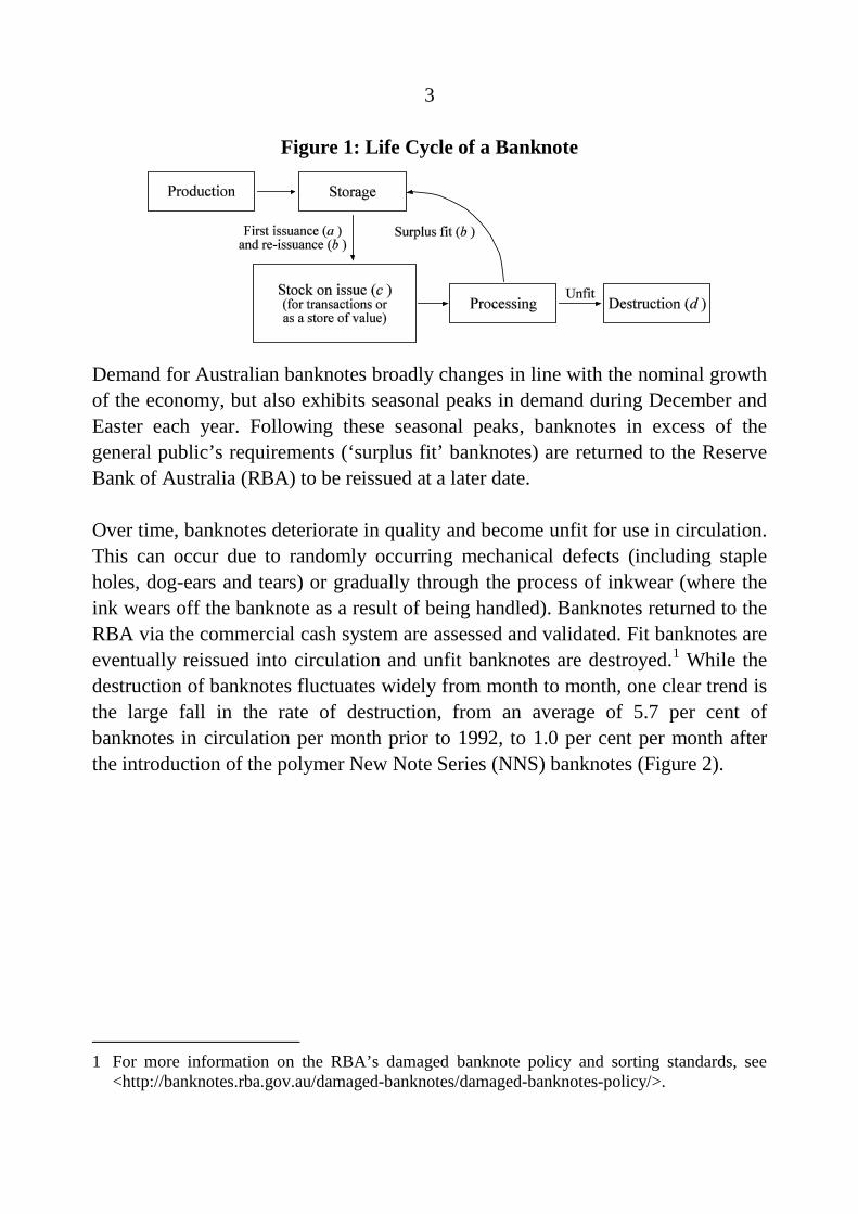
A banknote’s life begins with its production (Figure 1). Once produced, banknotes are held in storage until they are issued to the public. The elapsed time between production and issuance can vary considerably depending on the volume of banknotes produced in each banknote vintage (production year) and on fluctuations in the demand for banknotes. Once issued, banknotes may spend periods of time actively circulating or being held as a store of value.

3

Figure 1: Life Cycle of a Banknote

Demand for Australian banknotes broadly changes in line with the nominal growth of the economy, but also exhibits seasonal peaks in demand during December and Easter each year. Following these seasonal peaks, banknotes in excess of the general public’s requirements (‘surplus fit’ banknotes) are returned to the Reserve Bank of Australia (RBA) to be reissued at a later date.

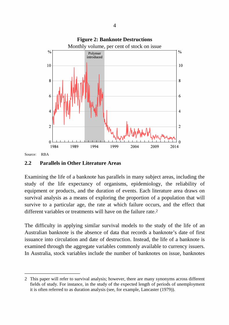
Over time, banknotes deteriorate in quality and become unfit for use in circulation. This can occur due to randomly occurring mechanical defects (including staple holes, dog-ears and tears) or gradually through the process of inkwear (where the ink wears off the banknote as a result of being handled). Banknotes returned to the RBA via the commercial cash system are assessed and validated. Fit banknotes are eventually reissued into circulation and unfit banknotes are destroyed.1 While the destruction of banknotes fluctuates widely from month to month, one clear trend is the large fall in the rate of destruction, from an average of 5.7 per cent of banknotes in circulation per month prior to 1992, to 1.0 per cent per month after the introduction of the polymer New Note Series (NNS) banknotes (Figure 2).

1 For more information on the RBA’s damaged banknote policy and sorting standards, see

<http://banknotes.rba.gov.au/damaged-banknotes/damaged-banknotes-policy/>.

4

Figure 2: Banknote Destructions Monthly volume, per cent of stock on issue

Source: RBA

2.2 Parallels in Other Literature Areas

Examining the life of a banknote has parallels in many subject areas, including the study of the life expectancy of organisms, epidemiology, the reliability of equipment or products, and the duration of events. Each literature area draws on survival analysis as a means of exploring the proportion of a population that will survive to a particular age, the rate at which failure occurs, and the effect that different variables or treatments will have on the failure rate.2

The difficulty in applying similar survival models to the study of the life of an Australian banknote is the absence of data that records a banknote’s date of first issuance into circulation and date of destruction. Instead, the life of a banknote is examined through the aggregate variables commonly available to currency issuers. In Australia, stock variables include the number of banknotes on issue, banknotes

2 This paper will refer to survival analysis; however, there are many synonyms across different

fields of study. For instance, in the study of the expected length of periods of unemployment it is often referred to as duration analysis (see, for example, Lancaster (1979)).

5

that have not been previously issued and surplus fit banknotes, and flow variables include the number of banknotes issued and destroyed.

2.3 Characterising the Deterioration of Banknotes

The survival analysis literature uses specialist terms for precisely describing the duration of events, such as banknote life. These terms avoid the ambiguities that arise with everyday expressions such as ‘life’ or ‘destruction rate’. The survival function measures the probability that the terminal date (in this case, when the banknote becomes unfit and is destroyed), denoted by the random variable T, is greater than a particular time, t. For example, the probability that a $50 banknote will last at least 15 years is estimated to be around 40 per cent (see Figure 6). Formally, the survival function is given by:

( ) ( ).S t P T t= > (1)

The complement of the survival function is the lifetime distribution function, which measures the probability that a banknote will be destroyed before or at a particular point in time.

( ) ( ) ( )1 .L t S t P T t= − = ≤ (2)

The derivative of the lifetime distribution function gives the event density function, which in this paper will be called the destruction function. Roughly speaking, the destruction function can be thought of as the rate at which banknotes are destroyed at a particular point in time.

( ) ( ) .dL t

l tdt

= (3)

The hazard function is defined as the event density at time t, given survival up to that point in time. This can be roughly interpreted as the rate at which banknotes will become unfit at a particular time, given survival up to that time. For example, 0.2 per cent of $50 banknotes that survive 20 years are then destroyed in that year.

( ) ( ) ( )/ .h t l t S t= (4)

6

Measures of the central tendency of a banknote’s useful life, such as their mean and median life when issued, are important for decision-making and can be derived from the above functions. In particular, these measures can help to inform banknote production decisions that are typically made years in advance. It should be clear, however, that these measures of expected life at issuance are different to the mean or median age of banknotes that are currently in circulation.

2.4 The Expected Shape of Hazard Functions

A banknote’s hazard function will be influenced by the two broad ways in which it can become unfit:

1. Mechanical defects are largely randomly occurring, or in other words, the probability that a banknote becomes unfit due to such a defect is invariant to the time that the banknote has been on issue. This corresponds with a constant hazard function.

2. Inkwear is a time-variant defect, since the probability that a banknote suffers sufficient levels of inkwear to be deemed unfit increases with the time spent in circulation. As such, inkwear gives rise to an increasing hazard function.

Given that these two categories of defects can occur, a banknote’s hazard function is expected to increase with respect to time since first issuance.

The preceding discussion refers to the hazard function of a given banknote; however, the average hazard rate of a group of banknotes may behave differently. One important factor is heterogeneity in the use of banknotes. Even though Australian banknotes are homogeneous, in that they are all made with the same materials and production processes over time, banknotes can be used for different purposes that affect their survival characteristics. Banknotes used repeatedly for transaction purposes are likely to have relatively high hazard rates, consistent with the fact that they are likely to experience greater inkwear or be subject to a random hazard such as stapling. On the other hand, some banknotes are used as a store of value or kept for numismatic purposes, and are therefore held in a protected location where they are much less likely to suffer inkwear or a mechanical defect. Such banknotes are likely to have very low hazard rates and are unlikely to become

7

unfit within the life of the banknote series. It is well-established in the survival analysis literature that if a population is composed of groups with differing hazard rates, even if the groups have constant or rising hazards, the aggregate hazard function could appear to be downward sloping, or rise then fall.3 More specific to the problem at hand, it has long been recognised in the medical literature (see Boag (1949) and Berkson and Gage (1952)) that having a proportion of long-term survivors in the population (i.e. individuals that don’t suffer the event of interest within the period of study) induces a longer tail in the survival distribution and a downward bias in estimates of the aggregate hazard rate.

Another complicating factor is that the hazard rates observed by the currency issuer could be lower due to the process of detecting unfit banknotes in circulation. Unfit banknotes are predominantly detected when banknotes that are surplus to demand are returned to the commercial cash system and sorted, which means that detection rates will be affected by the rate at which banknotes return for processing. Banknotes may also continue to circulate while unfit since whether a banknote is considered no longer fit for purpose is subjective and can vary considerably from person to person.

3. Traditional Steady-state or Turnover Method

The most common method that currency issuers use to estimate banknote life is a simple formula: the stock of banknotes on issue (averaged over a 12-month period) relative to the total number of banknotes destroyed (in the same 12-month period). Referring to Figure 1, the formula corresponds to dividing c by d. It is commonly termed the ‘steady-state’ method since it was thought that after a banknote series had been in circulation for a number of years, the growth in banknote destructions and circulation would reach stable levels, allowing for a steady-state estimate of banknote life. The formula is analogous to a turnover rate and measures the average number of years required to replace the current stock of banknotes in circulation if the current rate of destruction continues, thus estimating the useful life of the current stock of banknotes on issue. 3 As a simple example, consider a population composed of two groups – one with a high

constant hazard and one with a low constant hazard. If the two groups are not observed, on the aggregate level it will appear that the population’s hazard rate is declining since the high hazard group will fail more quickly, and over time the surviving population will have a higher and higher ratio of low hazard individuals.

8

12 .12

Mean Mean stock of banknotesonissueover mths cbanknotelife Total noof banknotes destroyed over mths d

= = (5)

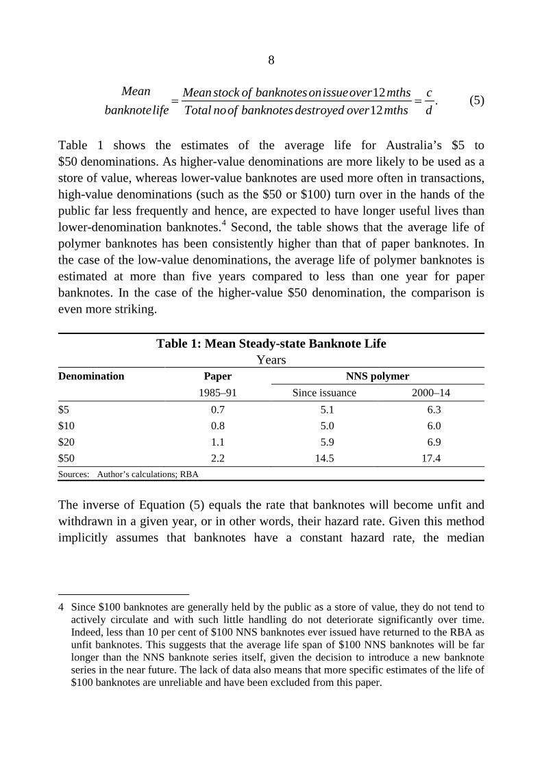
Table 1 shows the estimates of the average life for Australia’s $5 to $50 denominations. As higher-value denominations are more likely to be used as a store of value, whereas lower-value banknotes are used more often in transactions, high-value denominations (such as the $50 or $100) turn over in the hands of the public far less frequently and hence, are expected to have longer useful lives than lower-denomination banknotes.4 Second, the table shows that the average life of polymer banknotes has been consistently higher than that of paper banknotes. In the case of the low-value denominations, the average life of polymer banknotes is estimated at more than five years compared to less than one year for paper banknotes. In the case of the higher-value $50 denomination, the comparison is even more striking.

Table 1: Mean Steady-state Banknote Life Years

Denomination Paper NNS polymer 1985–91 Since issuance 2000–14 $5 0.7 5.1 6.3 $10 0.8 5.0 6.0 $20 1.1 5.9 6.9 $50 2.2 14.5 17.4 Sources: Author’s calculations; RBA

The inverse of Equation (5) equals the rate that banknotes will become unfit and withdrawn in a given year, or in other words, their hazard rate. Given this method implicitly assumes that banknotes have a constant hazard rate, the median

4 Since $100 banknotes are generally held by the public as a store of value, they do not tend to

actively circulate and with such little handling do not deteriorate significantly over time. Indeed, less than 10 per cent of $100 NNS banknotes ever issued have returned to the RBA as unfit banknotes. This suggests that the average life span of $100 NNS banknotes will be far longer than the NNS banknote series itself, given the decision to introduce a new banknote series in the near future. The lack of data also means that more specific estimates of the life of $100 banknotes are unreliable and have been excluded from this paper.

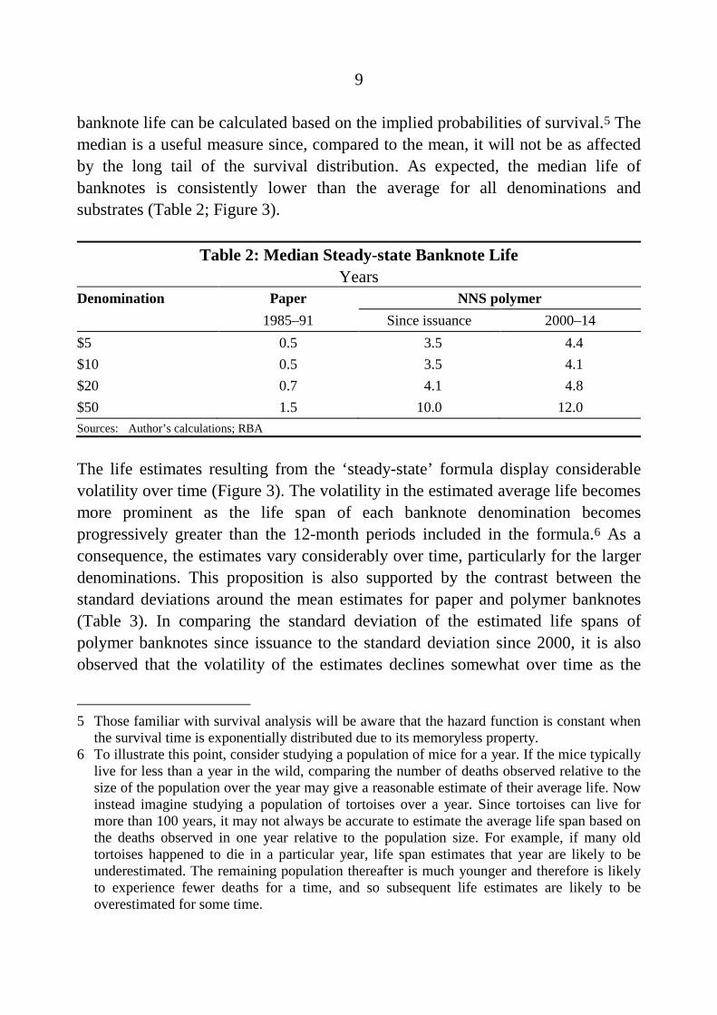
9

banknote life can be calculated based on the implied probabilities of survival.5 The median is a useful measure since, compared to the mean, it will not be as affected by the long tail of the survival distribution. As expected, the median life of banknotes is consistently lower than the average for all denominations and substrates (Table 2; Figure 3).

Table 2: Median Steady-state Banknote Life Years

Denomination Paper NNS polymer 1985–91 Since issuance 2000–14 $5 0.5 3.5 4.4 $10 0.5 3.5 4.1 $20 0.7 4.1 4.8 $50 1.5 10.0 12.0 Sources: Author’s calculations; RBA

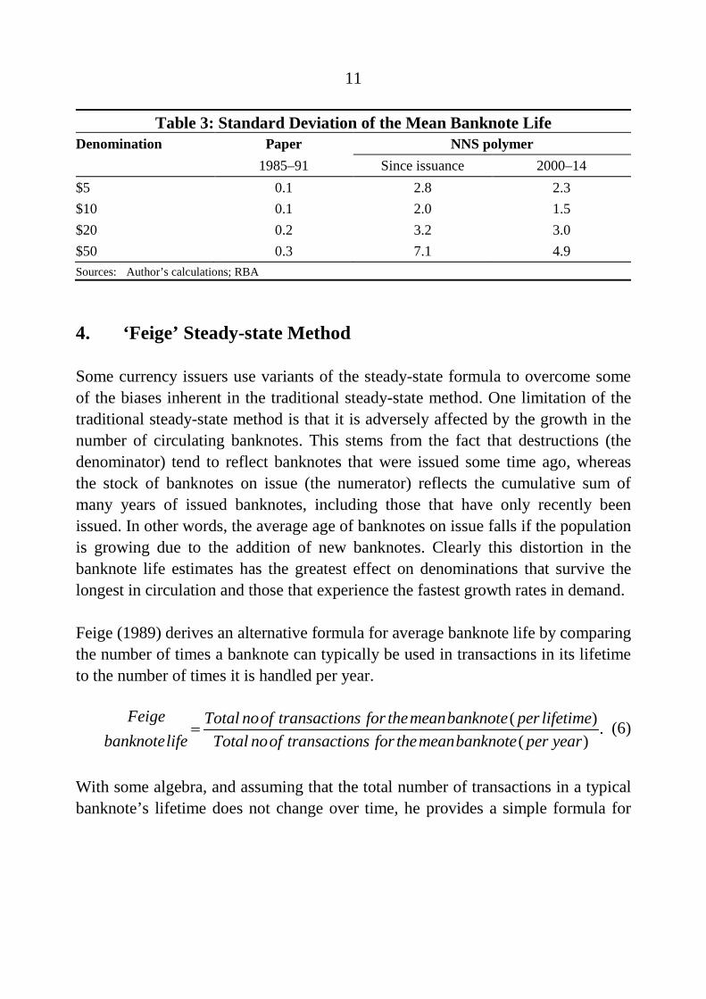
The life estimates resulting from the ‘steady-state’ formula display considerable volatility over time (Figure 3). The volatility in the estimated average life becomes more prominent as the life span of each banknote denomination becomes progressively greater than the 12-month periods included in the formula.6 As a consequence, the estimates vary considerably over time, particularly for the larger denominations. This proposition is also supported by the contrast between the standard deviations around the mean estimates for paper and polymer banknotes (Table 3). In comparing the standard deviation of the estimated life spans of polymer banknotes since issuance to the standard deviation since 2000, it is also observed that the volatility of the estimates declines somewhat over time as the

5 Those familiar with survival analysis will be aware that the hazard function is constant when

the survival time is exponentially distributed due to its memoryless property. 6 To illustrate this point, consider studying a population of mice for a year. If the mice typically

live for less than a year in the wild, comparing the number of deaths observed relative to the size of the population over the year may give a reasonable estimate of their average life. Now instead imagine studying a population of tortoises over a year. Since tortoises can live for more than 100 years, it may not always be accurate to estimate the average life span based on the deaths observed in one year relative to the population size. For example, if many old tortoises happened to die in a particular year, life span estimates that year are likely to be underestimated. The remaining population thereafter is much younger and therefore is likely to experience fewer deaths for a time, and so subsequent life estimates are likely to be overestimated for some time.

10

population increasingly includes banknotes across the full range of the survival distribution.

Figure 3: Steady-state Banknote Life

Sources: Author’s calculations; RBA

11

Table 3: Standard Deviation of the Mean Banknote Life Denomination Paper NNS polymer 1985–91 Since issuance 2000–14 $5 0.1 2.8 2.3 $10 0.1 2.0 1.5 $20 0.2 3.2 3.0 $50 0.3 7.1 4.9 Sources: Author’s calculations; RBA

4. ‘Feige’ Steady-state Method

Some currency issuers use variants of the steady-state formula to overcome some of the biases inherent in the traditional steady-state method. One limitation of the traditional steady-state method is that it is adversely affected by the growth in the number of circulating banknotes. This stems from the fact that destructions (the denominator) tend to reflect banknotes that were issued some time ago, whereas the stock of banknotes on issue (the numerator) reflects the cumulative sum of many years of issued banknotes, including those that have only recently been issued. In other words, the average age of banknotes on issue falls if the population is growing due to the addition of new banknotes. Clearly this distortion in the banknote life estimates has the greatest effect on denominations that survive the longest in circulation and those that experience the fastest growth rates in demand.

Feige (1989) derives an alternative formula for average banknote life by comparing the number of times a banknote can typically be used in transactions in its lifetime to the number of times it is handled per year.

( ) .( )

Feige Total noof transactions for themeanbanknote per lifetimebanknotelife Total noof transactions for themeanbanknote per year

= (6)

With some algebra, and assuming that the total number of transactions in a typical banknote’s lifetime does not change over time, he provides a simple formula for

12

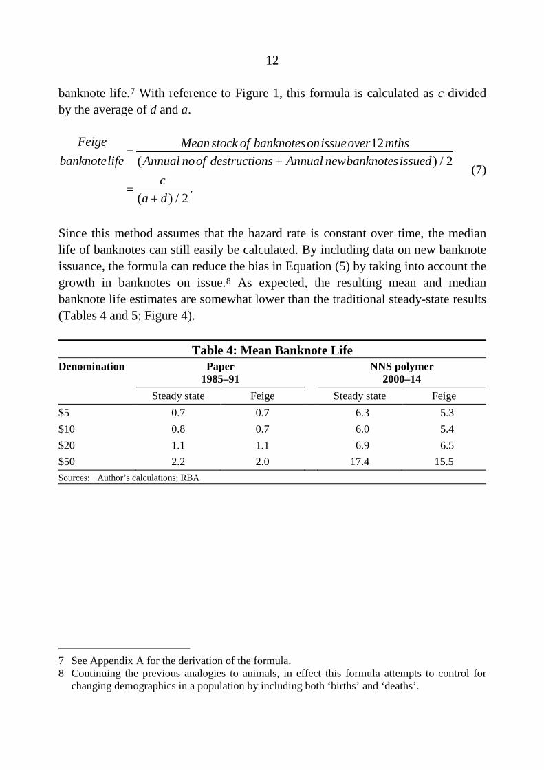
banknote life.7 With reference to Figure 1, this formula is calculated as c divided by the average of d and a.

12( ) / 2

.( ) / 2

Feige Mean stock of banknotesonissueover mthsbanknotelife Annual noof destructions Annual newbanknotesissued

ca d

=+

=+

(7)

Since this method assumes that the hazard rate is constant over time, the median life of banknotes can still easily be calculated. By including data on new banknote issuance, the formula can reduce the bias in Equation (5) by taking into account the growth in banknotes on issue.8 As expected, the resulting mean and median banknote life estimates are somewhat lower than the traditional steady-state results (Tables 4 and 5; Figure 4).

Table 4: Mean Banknote Life Denomination Paper

1985–91 NNS polymer

2000–14 Steady state Feige Steady state Feige

$5 0.7 0.7 6.3 5.3 $10 0.8 0.7 6.0 5.4 $20 1.1 1.1 6.9 6.5 $50 2.2 2.0 17.4 15.5 Sources: Author’s calculations; RBA

7 See Appendix A for the derivation of the formula. 8 Continuing the previous analogies to animals, in effect this formula attempts to control for

changing demographics in a population by including both ‘births’ and ‘deaths’.

13

Table 5: Median Banknote Life Denomination Paper




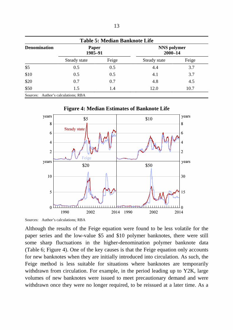
Figure 4: Median Estimates of Banknote Life


Although the results of the Feige equation were found to be less volatile for the paper series and the low-value $5 and $10 polymer banknotes, there were still some sharp fluctuations in the higher-denomination polymer banknote data (Table 6; Figure 4). One of the key causes is that the Feige equation only accounts for new banknotes when they are initially introduced into circulation. As such, the Feige method is less suitable for situations where banknotes are temporarily withdrawn from circulation. For example, in the period leading up to Y2K, large volumes of new banknotes were issued to meet precautionary demand and were withdrawn once they were no longer required, to be reissued at a later time. As a

14

result, there was a sharp decline in the estimated banknote life in 1999 and a sharp increase a year later.

Table 6: Standard Deviation of the Mean Banknote Life Denomination Paper




5. Limitations of the Steady-state Methods

The traditional and Feige steady-state methods are subject to several limitations. Both methods assume that the probability of a banknote becoming unfit is the same for all banknotes on issue regardless of their age, or in other words, they assume a constant hazard function. However, since the discussion in Section 2.4 indicated that the aggregate hazard rate is likely to vary with the time since issuance, this assumption is not likely to provide the best fit to the data.

Also, neither method is able to readily accommodate exogenous shocks to the number of banknotes on issue or changes in supply-side policies on the part of the currency issuer. Feige (1989) also identifies that an underlying assumption of his equation is that the total number of transactions in the average banknote’s lifetime does not change over time. Over the past twenty or so years, however, there have been a number of exogenous shocks, as follows.

5.1 Demand Shocks

Events which result in temporary fluctuations in the public’s demand for banknotes can adversely affect the steady-state measures of banknote quality. Two examples include Y2K and the GFC where the public’s demand for banknotes increased substantially. Even though shocks of this nature are often temporary, the impact on the number of banknotes in circulation can persist and distort banknote life

15

estimates for several years. For example, in late 2008, the demand for $50 banknotes increased sharply in response to the GFC. Although GFC concerns quickly abated, the number of $50 banknotes in circulation took more than two years to unwind. Reflecting this sharp increase in circulating $50 banknotes, banknote life (as estimated by Equations (5) and (7)) increased and remained at that higher level for several years (Figure 3).

5.2 Banknote Quality Programs

Implicit in the steady-state methods is an assumption that the currency issuer’s banknote quality programs are unchanged. This is somewhat unrealistic, however, as currency issuers are continually looking for opportunities to enhance the quality of banknotes in circulation. These improvements may take the form of new arrangements with banks and cash-in-transit companies (such as the Note Quality Reward Scheme introduced in Australia in 2006) or targeted ‘cleansing’ programs, which involve the accelerated replacement (and destruction) of specific denominations in circulation.9 Irrespective of the nature of the change, the outcome is the same; initially banknote life would appear to be low as destructions would be high relative to the stock of banknotes on issue, but banknote life would be higher in subsequent periods due to the higher quality of the remaining stock of banknotes on issue. Examples of the effect of cleansing programs can be clearly seen in the data for the $20 banknotes in 2006 and 2007, for the $10 banknotes in 2009 and 2010, and for the $5 in 2011 (Figure 3).

5.3 New Banknote Series

When a new series of banknotes is introduced into circulation, old series banknotes are withdrawn and destroyed. With a sharp increase in banknote issuances and destructions, the steady-state methods suggest a sharp decline in banknote life. This decline will be quickly offset, however, as the relatively higher-quality banknotes from the new series will circulate for a considerable period before being withdrawn. This profile is especially dramatic for banknotes that tend to have an average life in excess of the 12-month periods examined in the turnover formulas, which helps to explain the change in the banknote life profile of the $50 banknotes after the introduction of polymer banknotes in the mid 1990s (Figure 3). 9 For more information on the Note Quality Reward Scheme, see Cowling and Howlett (2012).

16

5.4 Cash Management

Underlying the steady-state methods is an assumption that the cash management arrangements between the currency issuer and the wholesale cash industry are unchanged. To a large extent this assumption is realistic, as changes to these arrangements tend to be incremental and have a negligible impact on banknote life estimates. In the case of Australia, however, the changes to the cash management arrangements in 2001 were sufficiently large that they did affect the steady-state estimates. In addition to changing the manner in which unfit banknotes were withdrawn from circulation and destroyed, some precautionary banknote holdings were transferred from the RBA to the commercial banks. Privatising these banknote holdings to the commercial banks resulted in a permanent increase in the number of banknotes measured as ‘on issue’, thereby leading to an increase in the average banknote life estimated by the steady-state formulas.

6. Survival Modelling

In order to address some of the limitations of the steady-state and Feige methods, I estimate survival models for banknote life, which can be used to derive the survival, hazard and destruction functions. The models provide estimates of many features of banknote survival, including the rates at which banknotes are likely to become unfit and measures of central tendency for banknote life spans. Accessible introductions to survival analysis are available in Jenkins (2008) and Wooldridge (2010).

Since there are no data recording the dates of issuance and destruction for samples of Australian banknotes, I utilise the data on aggregate issuance and destructions to estimate survival models. Importantly, the models can include explanatory variables that control for events such as demand shocks and changes to a currency issuer’s policies.

6.1 Model Specification

The survival function can be estimated by using the relationship between the actual and expected number of fit banknotes. It is important to note that fit banknotes include all banknotes on issue as well as surplus fit banknotes held by the currency

17

issuer.10 The actual number of fit banknotes is assumed to be equal to the total number of banknotes ever issued minus the total number of banknotes that have been destroyed up to that point in time.11

( )1

t

t n nn

F I D=

= −∑ (8)

where Ft is the total number of fit banknotes at time t, It is the number of new banknotes issued at time t, and Dt is the number of destructions at time t.

The expected number of fit banknotes at a particular point in time is equal to the sum of each new issuance since banknote production began, multiplied by each issuance’s survival function – that is the fraction of banknotes from each issuance date that are still likely to be fit for purpose at time t. The expected number of fit banknotes, based on the aggregate data, is given by:

( ) ( )1

;t

t n nn

E F S It=

= ∑ α (9)

where S( ) is the survival function, τt equals the amount of time since the first issuance of banknotes issued at t, and α equals a vector of parameters for survival function S.

Treating the difference between Ft and E(Ft) as a nonlinear regression residual, we can use nonlinear least squares to estimate the parameter vector α that governs the shape of the survival function, as shown in Equation (10). In other words, the actual number of fit banknotes from Equation (8) should be approximately equal to the expected number of banknotes from Equation (9). Differences between the two measures of fit banknotes may arise due to factors that cannot be included in the survival model, including changes in the public’s treatment of banknotes,

10 Surplus fit banknotes are those that have previously circulated but are surplus to public

demand. 11 This assumption is reasonable if the majority of banknotes that become unfit are returned for

destruction. Otherwise, if a large proportion of banknotes are lost or destroyed while in circulation the number of fit banknotes will be overstated.

18

preferences for different payment instruments, or changes in the policies of the commercial cash sector.

( )

( )1

;

t t t

t

t n n tn

F E F

F S I

ε

t ε=

= +

= +∑ α (10)

where εt is an error term.

I investigated a range of different specifications for the survival function in Equation (10). I found that results based on Weibull survival distributions, which have two parameters that determine the scale (λ) and shape (k) of the distribution, were the most plausible. This distribution is commonly used in the survival analysis literature and is flexible in that the estimated hazard function can be monotonically increasing (when λ is greater than one), monotonically decreasing (when λ is less than one) or a constant (when λ equals one). Log-logistic specifications were also examined since they allow the hazard function to vary non-monotonically, but this property did not seem to be empirically important.

The specification in Equation (10) can also be extended in two ways. First, the discussion in Section 2.4 indicated that it may be important to take into account the potential for unobserved heterogeneity in the use of banknotes. Rather than assuming that all banknotes will eventually become unfit, we can split the population of banknotes into two groups: banknotes that become worn and are eventually returned for destruction; and banknotes that will not be returned within the life of the banknote series, which could include banknotes that are held for precautionary or numismatic purposes. The probability that a banknote returns for destruction (p) can be incorporated in the models as an extra parameter to be estimated.

Second, explanatory variables can be introduced to take into account factors that impact the issuance, durability and destruction of banknotes to help address some of the shortcomings of the two steady-state methods. These variables can be included such that they interact with the hazard function multiplicatively, in a similar way to the proportional hazards models that are common in the survival analysis literature. The specific variables included in the survival models vary

19

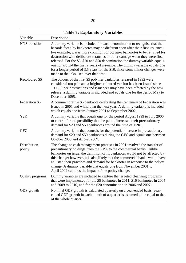
across denominations (Table 7). Dummy variables are included to control for the RBA’s quality programs which targeted the $5, $10 and $20 denominations. The change to the distribution arrangements in 2001, which involved the privatisation of some banknote holdings, are more relevant to the higher value $20 and $50 denominations, as are the shocks to demand.

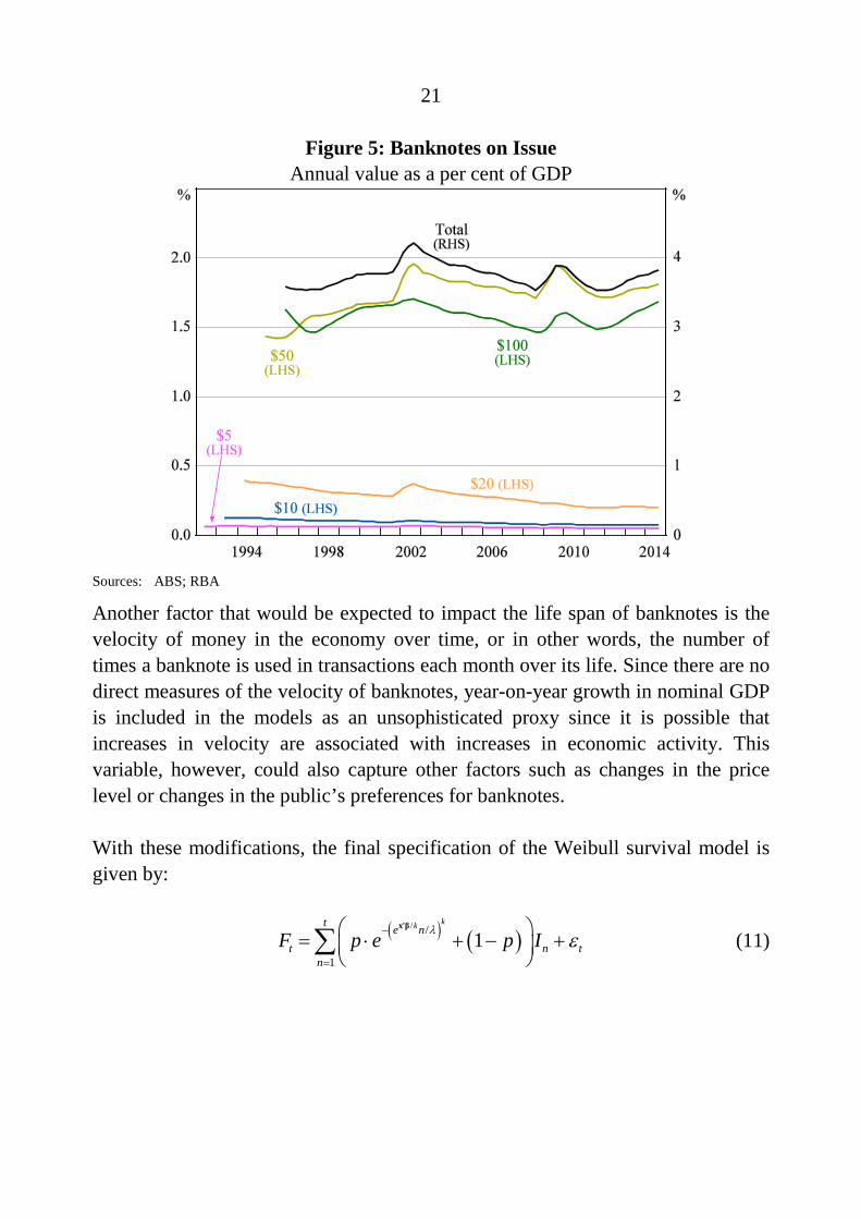
The usage of different denominations in automated teller machines (ATMs) over time could also be suggested as a sensible variable to include in the models, as it could capture shifts in the public’s treatment of different denominations. The number or proportion of different denominations used in ATMs, however, is not known. Since changes to the denominations used in ATMs were not coordinated across institutions, it would also be difficult to construct accurate dummy variables. Observing the yearly issuance patterns after the distribution of polymer banknotes (from 1992 for the $5 to 1996 for the $100), it is reassuring to note that there does not appear to be any sudden structural shifts in the composition of banknotes on issue (Figure 5). It is evident that there are some gradual trends in the composition of banknotes on issue over time (such as an increasing prominence of $50 banknotes and a decline in the share of $20 banknotes). These trends would be important if they are associated with a shift in the public’s treatment of banknotes; however, given the stability of the survival model’s estimates over time this does not seem to be a concern (Figure 7).

20

Table 7: Explanatory Variables Variable Description NNS transition A dummy variable is included for each denomination to recognise that the

hazards faced by banknotes may be different soon after their first issuance. For example, it was more common for polymer banknotes to be returned for destruction with deliberate scratches or other damage when they were first released. For the $5, $20 and $50 denomination the dummy variable equals one for around the first 2 years of issuance. The dummy variable equals one for a longer period of 3.5 years for the $10, since some minor changes were made to the inks used over that time.

Recoloured $5 The colours of the first $5 polymer banknotes released in 1992 were considered too pale and a brighter coloured version has been issued since 1995. Since destructions and issuances may have been affected by the new release, a dummy variable is included and equals one for the period May to December 1995.

Federation $5 A commemorative $5 banknote celebrating the Centenary of Federation was issued in 2001 and withdrawn the next year. A dummy variable is included, which equals one from January 2001 to September 2002.

Y2K A dummy variable that equals one for the period August 1999 to July 2000 to control for the possibility that the public increased their precautionary demand for $20 and $50 banknotes around the time of Y2K.

GFC A dummy variable that controls for the potential increase in precautionary demand for $20 and $50 banknotes during the GFC and equals one between October 2008 and August 2009.

Distribution policy

The change to cash management practises in 2001 involved the transfer of precautionary holdings from the RBA to the commercial banks. Unlike banknotes on issue, the definition of fit banknotes would not be affected by this change; however, it is also likely that the commercial banks would have adjusted their practices and demand for banknotes in response to the policy change. A dummy variable that equals one from November 2001 to April 2002 captures the impact of the policy change.

Quality programs Dummy variables are included to capture the targeted cleansing programs that were implemented for the $5 banknotes in 2011, $10 banknotes in 2005 and 2009 to 2010, and for the $20 denomination in 2006 and 2007.

GDP growth Nominal GDP growth is calculated quarterly on a year-ended basis; year-ended GDP growth in each month of a quarter is assumed to be equal to that of the whole quarter.

21

Figure 5: Banknotes on Issue Annual value as a per cent of GDP

Sources: ABS; RBA

Another factor that would be expected to impact the life span of banknotes is the velocity of money in the economy over time, or in other words, the number of times a banknote is used in transactions each month over its life. Since there are no direct measures of the velocity of banknotes, year-on-year growth in nominal GDP is included in the models as an unsophisticated proxy since it is possible that increases in velocity are associated with increases in economic activity. This variable, however, could also capture other factors such as changes in the price level or changes in the public’s preferences for banknotes.

With these modifications, the final specification of the Weibull survival model is given by:

( ) ( )/ /

11

kkt e nt n t

nF p e p Iλ ε−

=

= ⋅ + − +

∑x'β

(11)

22

where p is the probability of a banknote being returned for destruction12 and x'β equals a matrix of explanatory variables and their vector of coefficients.

Notice that in this specification, for any group of banknotes issued, there is a constant (1– p) mass of banknotes that in effect last for ever, and a constant mass, p, that are assumed to become unfit. Derivations of the associated hazard function, destruction function and measures of central tendency are found in Appendix B.

6.2 Survival Model Results

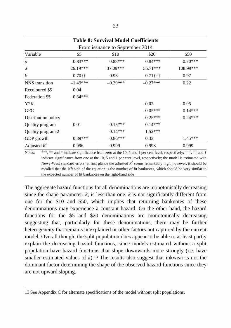
Estimates of the survival models are shown in Table 8. The value of p in the $50 model implies that at least 30 per cent of $50 banknotes will not become unfit. In comparison, the proportion of banknotes that will not become unfit is between 10 and 15 per cent for the lower-value denominations. The result that p is noticeably lower for the $5 compared to the $10 may not seem intuitive but there are a number of reasons that this may be the case. It is plausible that since the $5 is the lowest value denomination it is less likely to be looked after by the public and more likely to be lost or destroyed in circulation. It is also possible that more $5 banknotes are held for numismatic purposes since it was the first NNS denomination released, and since recoloured $5 and Federation $5 banknote designs were issued. To give a sense of scale – in the first year of the NNS series more than 80 million $5 banknotes were issued, around 35 million recoloured $5 were issued in their first year, and 70 million Federation $5 banknotes were issued over 2001 – only an extra 5 per cent of these $5 banknotes (or around 0.4 banknotes per capita) would have had to be held by the public to make up for the difference between the models’ estimates of p for the $5 and $10.

12 Technically, p is estimated using a logistic function so that its value is restricted to be

between zero and one.

23

Table 8: Survival Model Coefficients From issuance to September 2014

Variable $5 $10 $20 $50 p 0.83*** 0.88*** 0.84*** 0.70*** λ 26.19*** 37.09*** 55.71*** 108.99*** k 0.70†† 0.93 0.71††† 0.97 NNS transition –1.49*** –0.30*** –0.27*** 0.22 Recoloured $5 0.04 Federation $5 –0.34*** Y2K –0.02 –0.05 GFC –0.05*** 0.14*** Distribution policy –0.25*** –0.24*** Quality program 0.01 0.15*** 0.14*** Quality program 2 0.14*** 1.52*** GDP growth 0.89*** 0.86*** 0.33 1.45*** Adjusted R2 0.996 0.999 0.998 0.999 Notes: ***, ** and * indicate significance from zero at the 10, 5 and 1 per cent level, respectively; †††, †† and †

indicate significance from one at the 10, 5 and 1 per cent level, respectively; the model is estimated with Newy-West standard errors; at first glance the adjusted R2 seems remarkably high, however, it should be recalled that the left side of the equation is the number of fit banknotes, which should be very similar to the expected number of fit banknotes on the right-hand side

The aggregate hazard functions for all denominations are monotonically decreasing since the shape parameter, k, is less than one. k is not significantly different from one for the $10 and $50, which implies that returning banknotes of these denominations may experience a constant hazard. On the other hand, the hazard functions for the $5 and $20 denominations are monotonically decreasing suggesting that, particularly for these denominations, there may be further heterogeneity that remains unexplained or other factors not captured by the current model. Overall though, the split population does appear to be able to at least partly explain the decreasing hazard functions, since models estimated without a split population have hazard functions that slope downwards more strongly (i.e. have smaller estimated values of k).13 The results also suggest that inkwear is not the dominant factor determining the shape of the observed hazard functions since they are not upward sloping.

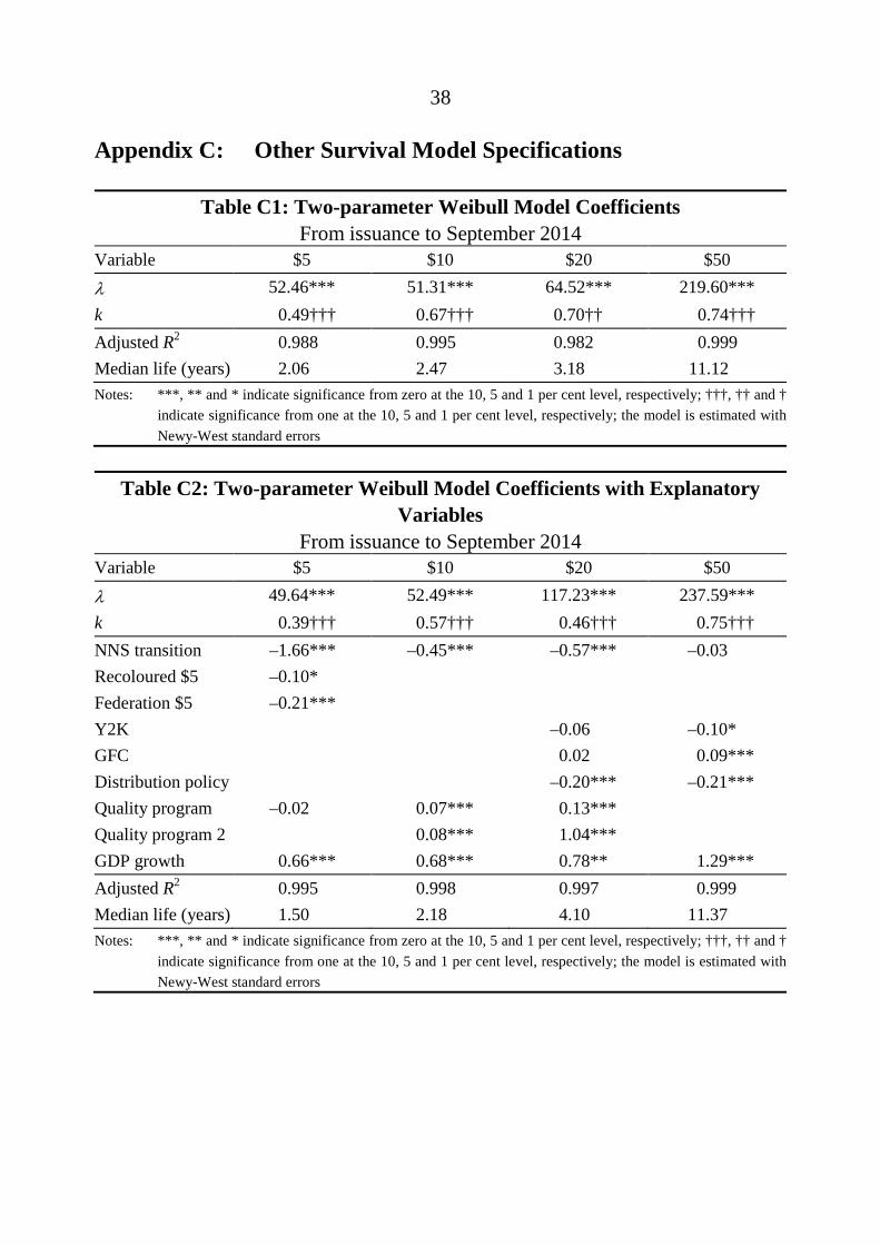
13 See Appendix C for alternate specifications of the model without split populations.

24

Examining the coefficients of the explanatory variables, the reduction in survival during the GFC suggests that $50 banknotes were not only held in greater numbers but were also used and handled more frequently. The economic significance of the GFC variable is not particularly large – a $50 banknote first issued during the GFC would be 1.2 per cent less likely to survive its first year of circulation than if the GFC had not occurred. On the other hand, Y2K did not have a statistically significant impact on the life span of $20 or $50 banknotes. As expected, the quality programs (which are associated with elevated banknote destruction rates) reduce the survival of banknotes during the period and are statistically significant for the $10 and $20 denominations. The GDP growth parameter is positive and significant across all denominations except the $20 (for which it is not statistically different from zero), indicating the intensity of cash usage increases with economic activity. Despite its statistical significance, however, the economic implication of this variable is small – for example, a newly issued $50 banknote would be 0.1 per cent less likely survive its first year in circulation if year-ended GDP growth was 4 rather than 3 per cent.

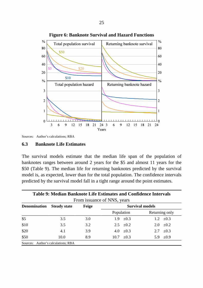
The coefficients of the models can be used to construct the survival and hazard functions for both the population of banknotes and for the sub-population of banknotes that will be returned as unfit (Figure 6).14 For both the population and the returning banknotes, the $50 banknotes have a higher survival rate compared to the other denominations and the $20 banknotes’ survival rate exceeds that of the lowest two denominations in all time periods. Looking at the sub-population of returning banknotes, it appears that the $10 banknotes survive longer than the $5 banknotes; however, for the total populations, a higher proportion of $5 banknotes survive in the long run due to their lower propensity to be returned for destruction. The hazard functions for the total populations of each banknote denomination are downward sloping and, as previously discussed, the hazard functions for the returning sub-populations of banknotes are close to constant for the $10 and $50, but still somewhat downward sloping for the $5 and $20.

14 A policymaker may, in some cases, be more interested in only the survival characteristics of

banknotes that will be returned for destruction for instance, when making decisions on the production volumes required for replacement.

25

Figure 6: Banknote Survival and Hazard Functions


6.3 Banknote Life Estimates

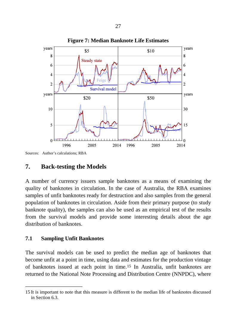
The survival models estimate that the median life span of the population of banknotes ranges between around 2 years for the $5 and almost 11 years for the $50 (Table 9). The median life for returning banknotes predicted by the survival model is, as expected, lower than for the total population. The confidence intervals predicted by the survival model fall in a tight range around the point estimates.

Table 9: Median Banknote Life Estimates and Confidence Intervals From issuance of NNS, years

Denomination Steady state Feige Survival models Population Returning only $5 3.5 3.0 1.9 ±0.3 1.2 ±0.3 $10 3.5 3.2 2.5 ±0.2 2.0 ±0.2 $20 4.1 3.9 4.0 ±0.3 2.7 ±0.3 $50 10.0 8.9 10.7 ±0.3 5.9 ±0.9 Sources: Author’s calculations; RBA

26

Looking more closely at the measures of central tendency across the different methodologies also provides some interesting insights (Table 9). The median banknote life estimates for all banknotes are most similar for the $50 denomination, whereas the estimates for the $5 are noticeably lower under the survival modelling framework. Across all of the models and measures, though, we observe the same pattern of longer life estimates as the denomination value increases. The differential between the useful life of the highest- and lowest-value denominations, however, is higher under the survival model’s estimates compared to the two steady-state methods.

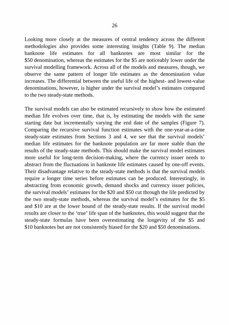
The survival models can also be estimated recursively to show how the estimated median life evolves over time, that is, by estimating the models with the same starting date but incrementally varying the end date of the samples (Figure 7). Comparing the recursive survival function estimates with the one-year-at-a-time steady-state estimates from Sections 3 and 4, we see that the survival models’ median life estimates for the banknote population are far more stable than the results of the steady-state methods. This should make the survival model estimates more useful for long-term decision-making, where the currency issuer needs to abstract from the fluctuations in banknote life estimates caused by one-off events. Their disadvantage relative to the steady-state methods is that the survival models require a longer time series before estimates can be produced. Interestingly, in abstracting from economic growth, demand shocks and currency issuer policies, the survival models’ estimates for the $20 and $50 cut through the life predicted by the two steady-state methods, whereas the survival model’s estimates for the $5 and $10 are at the lower bound of the steady-state results. If the survival model results are closer to the ‘true’ life span of the banknotes, this would suggest that the steady-state formulas have been overestimating the longevity of the $5 and $10 banknotes but are not consistently biased for the $20 and $50 denominations.

27

Figure 7: Median Banknote Life Estimates


7. Back-testing the Models

A number of currency issuers sample banknotes as a means of examining the quality of banknotes in circulation. In the case of Australia, the RBA examines samples of unfit banknotes ready for destruction and also samples from the general population of banknotes in circulation. Aside from their primary purpose (to study banknote quality), the samples can also be used as an empirical test of the results from the survival models and provide some interesting details about the age distribution of banknotes.

7.1 Sampling Unfit Banknotes

The survival models can be used to predict the median age of banknotes that become unfit at a point in time, using data and estimates for the production vintage of banknotes issued at each point in time.15 In Australia, unfit banknotes are returned to the National Note Processing and Distribution Centre (NNPDC), where

15 It is important to note that this measure is different to the median life of banknotes discussed

in Section 6.3.

28

they are validated, assessed and destroyed. A sample of around 800 000 unfit banknotes was extracted in 2011 and sorted into production vintages.16 These data were then compared to the composition of unfit banknotes predicted by the survival models and the traditional steady-state method.

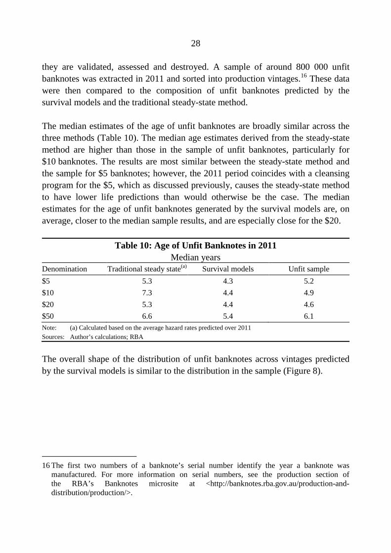
The median estimates of the age of unfit banknotes are broadly similar across the three methods (Table 10). The median age estimates derived from the steady-state method are higher than those in the sample of unfit banknotes, particularly for $10 banknotes. The results are most similar between the steady-state method and the sample for $5 banknotes; however, the 2011 period coincides with a cleansing program for the $5, which as discussed previously, causes the steady-state method to have lower life predictions than would otherwise be the case. The median estimates for the age of unfit banknotes generated by the survival models are, on average, closer to the median sample results, and are especially close for the $20.

Table 10: Age of Unfit Banknotes in 2011 Median years

Denomination Traditional steady state(a) Survival models Unfit sample $5 5.3 4.3 5.2 $10 7.3 4.4 4.9 $20 5.3 4.4 4.6 $50 6.6 5.4 6.1 Note: (a) Calculated based on the average hazard rates predicted over 2011 Sources: Author’s calculations; RBA

The overall shape of the distribution of unfit banknotes across vintages predicted by the survival models is similar to the distribution in the sample (Figure 8).

16 The first two numbers of a banknote’s serial number identify the year a banknote was

manufactured. For more information on serial numbers, see the production section of the RBA’s Banknotes microsite at <http://banknotes.rba.gov.au/production-and-distribution/production/>.

29

Figure 8: Unfit Banknotes in Survival Models and Sample Per cent of total, 2011


7.2 Sampling Banknotes in Circulation

A second sample methodology used by the Reserve Bank is the commercial cash sampling (CCS) program. This program involves taking samples of unsorted banknotes from cash-in-transit (CIT) companies across the country. Although the purpose of this program is to assess the quality of circulating banknotes, it also provides an opportunity to examine the vintages of banknotes in circulation.17

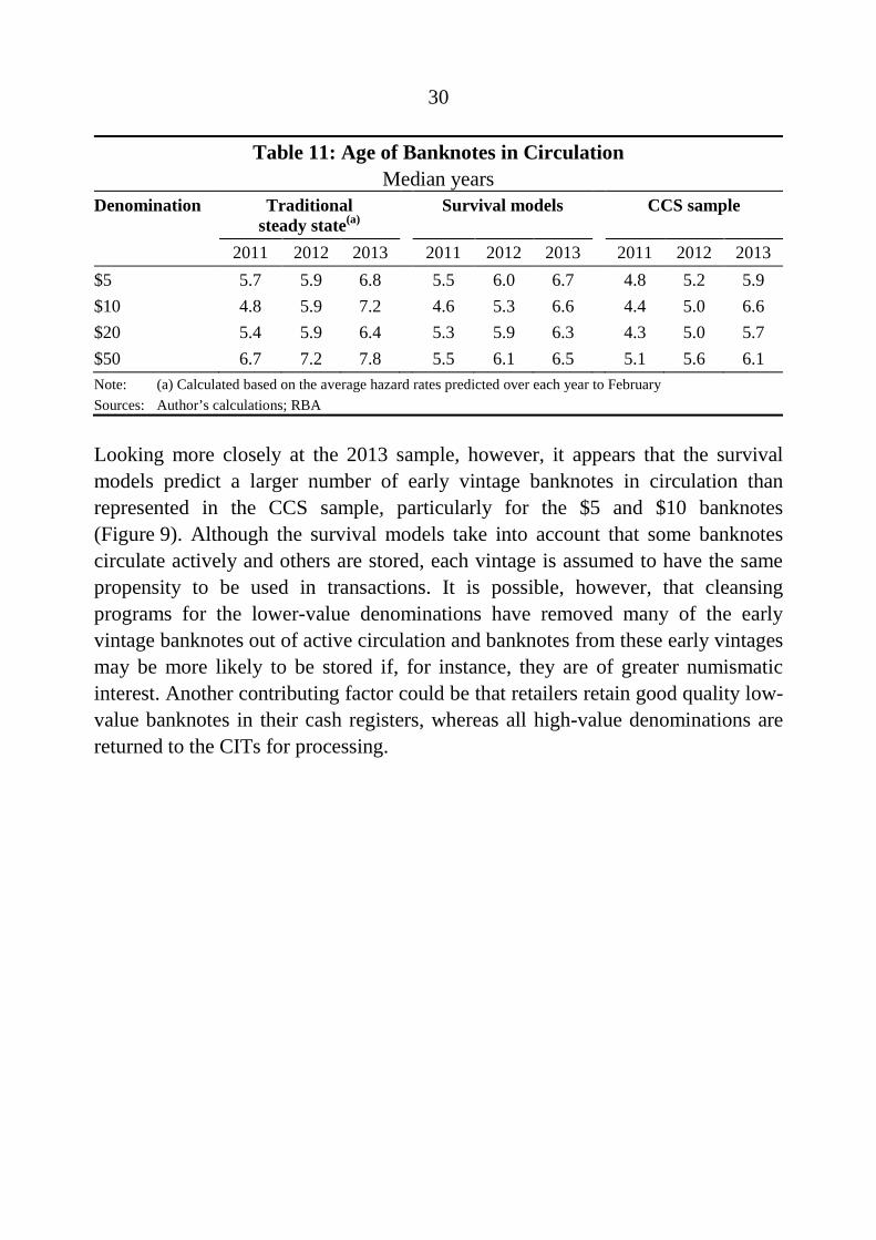
Examining three sample periods (February in each of 2011, 2012 and 2013) shows that the median ages of banknotes in circulation from the CCS samples tend to be closer to those predicted by the survival models (Table 11). Again, the traditional steady-state method tends to imply higher median ages for banknotes on issue than predicted by the survival models and the CCS sample.

17 It should be noted that with around two to three thousand banknotes collected for each

denomination, the samples are small relative to the stock of banknotes on issue and that the samples can only be drawn from the pool of banknotes that actively circulate.

30

Table 11: Age of Banknotes in Circulation Median years

Denomination Traditional steady state(a)

Survival models CCS sample

2011 2012 2013 2011 2012 2013 2011 2012 2013 $5 5.7 5.9 6.8 5.5 6.0 6.7 4.8 5.2 5.9 $10 4.8 5.9 7.2 4.6 5.3 6.6 4.4 5.0 6.6 $20 5.4 5.9 6.4 5.3 5.9 6.3 4.3 5.0 5.7 $50 6.7 7.2 7.8 5.5 6.1 6.5 5.1 5.6 6.1 Note: (a) Calculated based on the average hazard rates predicted over each year to February Sources: Author’s calculations; RBA

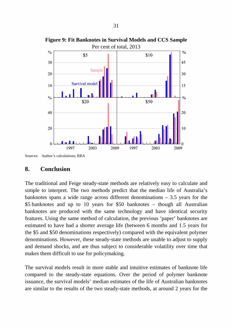
Looking more closely at the 2013 sample, however, it appears that the survival models predict a larger number of early vintage banknotes in circulation than represented in the CCS sample, particularly for the $5 and $10 banknotes (Figure 9). Although the survival models take into account that some banknotes circulate actively and others are stored, each vintage is assumed to have the same propensity to be used in transactions. It is possible, however, that cleansing programs for the lower-value denominations have removed many of the early vintage banknotes out of active circulation and banknotes from these early vintages may be more likely to be stored if, for instance, they are of greater numismatic interest. Another contributing factor could be that retailers retain good quality low-value banknotes in their cash registers, whereas all high-value denominations are returned to the CITs for processing.

31

Figure 9: Fit Banknotes in Survival Models and CCS Sample Per cent of total, 2013


8. Conclusion

The traditional and Feige steady-state methods are relatively easy to calculate and simple to interpret. The two methods predict that the median life of Australia’s banknotes spans a wide range across different denominations – 3.5 years for the $5 banknotes and up to 10 years for $50 banknotes – though all Australian banknotes are produced with the same technology and have identical security features. Using the same method of calculation, the previous ‘paper’ banknotes are estimated to have had a shorter average life (between 6 months and 1.5 years for the $5 and $50 denominations respectively) compared with the equivalent polymer denominations. However, these steady-state methods are unable to adjust to supply and demand shocks, and are thus subject to considerable volatility over time that makes them difficult to use for policymaking.

The survival models result in more stable and intuitive estimates of banknote life compared to the steady-state equations. Over the period of polymer banknote issuance, the survival models’ median estimates of the life of Australian banknotes are similar to the results of the two steady-state methods, at around 2 years for the

32

$5 denomination and almost 11 years for the $50 denomination. Although the survival models are more complex, they can be used to produce a range of interesting metrics other than the simple measures of central tendency, allowing a more in-depth exploration of banknote survival. The results suggest that the survival of banknotes is not only dependent on the ways in which banknotes become unfit, but on aggregate, they are also influenced by fluctuations in demand, the currency issuer’s choice of distribution or processing arrangements, and the dual use of banknotes (in transactions and as a store of value). Intuitively, the models showed that $50 banknotes are more likely to be used as a store of value as well as in transactions, whereas lower-value denominations are predominantly used in transactions.

Despite this, some questions over the true shape of the survival and hazard functions remain as it is quite likely that there is still some heterogeneity across banknote usage that cannot be captured by the current modelling techniques. In the future, technology improvements that make it possible to record the date of first issuance and destruction for each banknote would make it feasible to investigate this heterogeneity further using more conventional survival analysis techniques.

The sampling data collected through the RBA’s banknote quality programs provide a useful way to test and verify the age distribution of unfit and circulating banknotes predicted by the survival models. The age distribution of those banknotes in circulation and those that have been destroyed, as predicted by the steady-state methods and survival models, are generally similar to those in the two banknote samples. On average, however, the survival models’ predictions are closer to the outcomes of the banknote sampling programs.

33

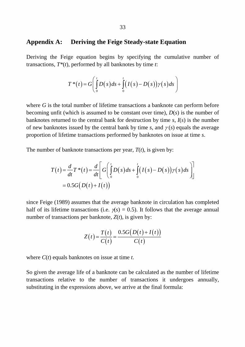
Appendix A: Deriving the Feige Steady-state Equation

Deriving the Feige equation begins by specifying the cumulative number of transactions, T*(t), performed by all banknotes by time t:

( ) ( ) ( ) ( )( ) ( )0 0

*t t

T t G D s ds I s D s s dsγ

= + − ∫ ∫

where G is the total number of lifetime transactions a banknote can perform before becoming unfit (which is assumed to be constant over time), D(s) is the number of banknotes returned to the central bank for destruction by time s, I(s) is the number of new banknotes issued by the central bank by time s, and γ (s) equals the average proportion of lifetime transactions performed by banknotes on issue at time s.

The number of banknote transactions per year, T(t), is given by:

( ) ( ) ( ) ( ) ( )( ) ( )

( ) ( )( )0 0

*

0.5

t td dT t T t G D s ds I s D s s dsdt dt

G D t I t

γ

= = + −

= +

∫ ∫

since Feige (1989) assumes that the average banknote in circulation has completed half of its lifetime transactions (i.e. γ(s) = 0.5). It follows that the average annual number of transactions per banknote, Z(t), is given by:

( ) ( )( )

( ) ( )( )( )

0.5G D t I tT tZ t

C t C t+

= =

where C(t) equals banknotes on issue at time t.

So given the average life of a banknote can be calculated as the number of lifetime transactions relative to the number of transactions it undergoes annually, substituting in the expressions above, we arrive at the final formula:

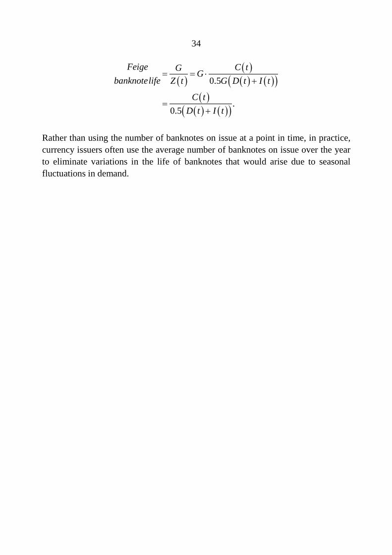
34

( )

( )( ) ( )( )

( )( ) ( )( )

0.5

.0.5

Feige C tG Gbanknotelife Z t G D t I t

C tD t I t

= = ⋅+

=+

Rather than using the number of banknotes on issue at a point in time, in practice, currency issuers often use the average number of banknotes on issue over the year to eliminate variations in the life of banknotes that would arise due to seasonal fluctuations in demand.

35

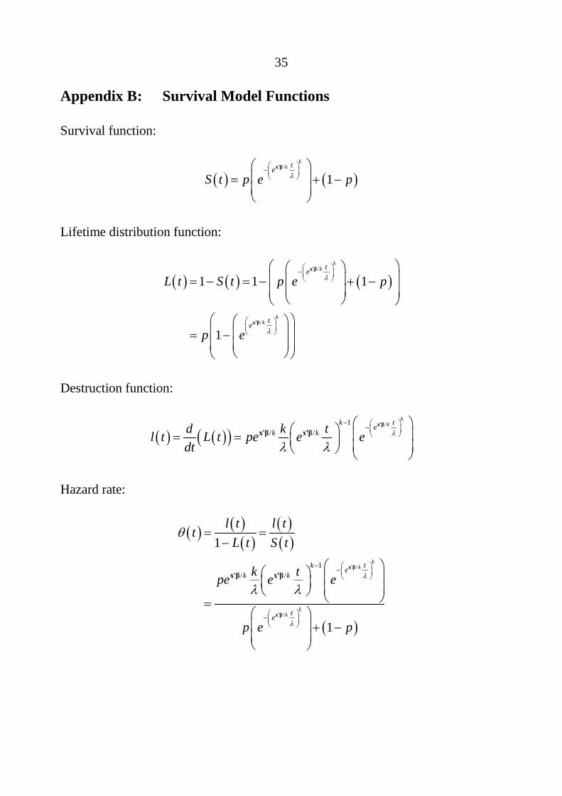
Appendix B: Survival Model Functions

Survival function:

( ) ( )/

1k

k teS t p e pλ

−

= + −

x'β

Lifetime distribution function:

( ) ( ) ( )/

/

1 1 1

1

kk

kk

te

te

L t S t p e p

p e

λ

λ

−

= − = − + −

= −

x'β

x'β

Destruction function:

( ) ( )( )/1

/ /

kkk te

k kd k tl t L t pe e edt

λ

λ λ

− −

= =

x'βx'β x'β

Hazard rate:

( ) ( )( )

( )( )

( )

/

/

1/ /

1

1

kk

kk

tk ek k

te

l t l tt

L t S t

k tpe e e

p e p

λ

λ

θ

λ λ

− −

−

= =−

= + −

x'β

x'β

x'β x'β

36

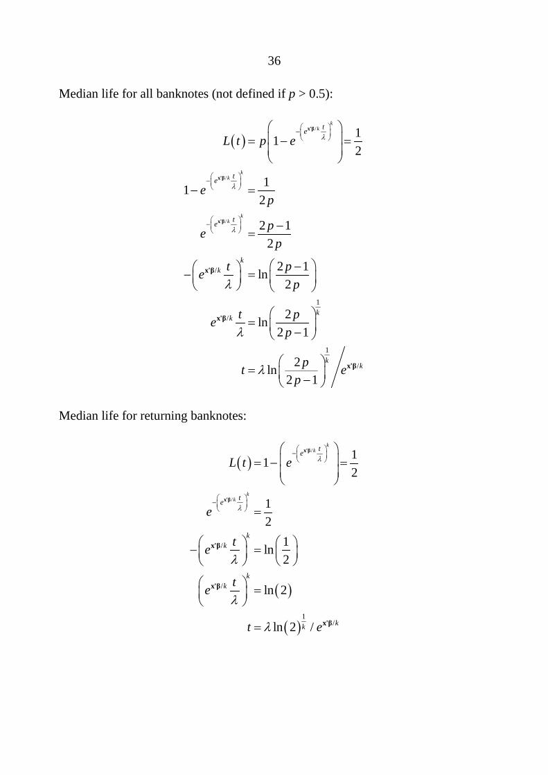
Median life for all banknotes (not defined if p > 0.5):

( )/

/

/

/

1

/

1

/

112

112

2 12

2 1ln2

2ln2 1

2ln2 1

kk

kk

kk

te

te

te

kk

kk

kk

L t p e

ep

pep

t pep

t pep

pt ep

λ

λ

λ

λ

λ

λ

−

−

−

= − =

− =

−=

− − =

= −

= −

x'β

x'β

x'β

x'β

x'β

x'β

Median life for returning banknotes:

( )

( )

( )

/

/

/

/

1/

112

12

1ln2

ln 2

ln 2 /

kk

kk

te

te

kk

kk

kk

L t e

e

te

te

t e

λ

λ

λ

λ

λ

−

−

= − =

=

− =

=

=

x'β

x'β

x'β

x'β

x'β

37

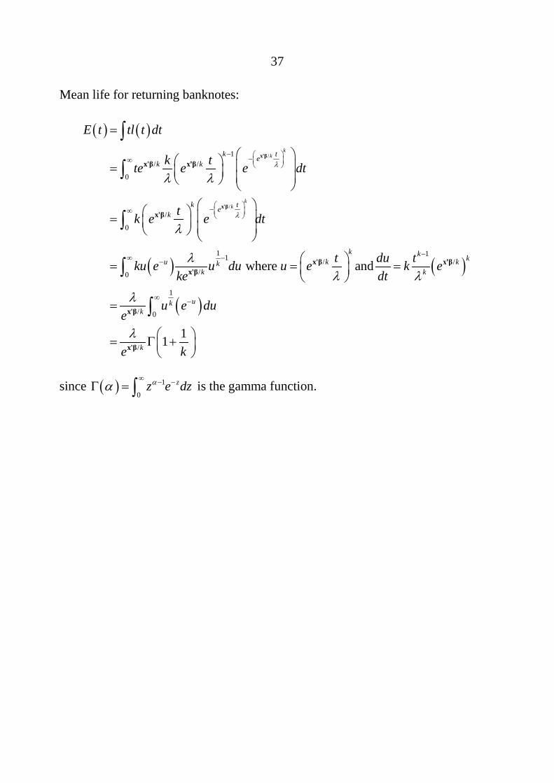
Mean life for returning banknotes:

( ) ( )

( ) ( )

( )

/

/

1/ /

0

/

0

1 11 / //0

1

/ 0

where and

kk

kk

k tek k

k tek

k k ku k kkk k

ukk

E t tl t dt

k tte e e dt

tk e e dt

t du tku e u du u e k eke dt

u e due

λ

λ

λ λ

λ

λλ λ

λ

− −∞

−∞

−−∞ −

∞ −

=

= =

= = =

=

∫

∫

∫

∫

∫

x'β

x'β

x'β x'β

x'β

x'β x'βx'β

x'β

/

11ke kλ = Γ +

x'β

since ( ) 1

0

zz e dzαα∞ − −Γ = ∫ is the gamma function.

38

Appendix C: Other Survival Model Specifications

Table C1: Two-parameter Weibull Model Coefficients From issuance to September 2014

Variable $5 $10 $20 $50 λ 52.46*** 51.31*** 64.52*** 219.60*** k 0.49††† 0.67††† 0.70†† 0.74††† Adjusted R2 0.988 0.995 0.982 0.999 Median life (years) 2.06 2.47 3.18 11.12 Notes: ***, ** and * indicate significance from zero at the 10, 5 and 1 per cent level, respectively; †††, †† and †

indicate significance from one at the 10, 5 and 1 per cent level, respectively; the model is estimated with Newy-West standard errors

Table C2: Two-parameter Weibull Model Coefficients with Explanatory

Variables From issuance to September 2014

Variable $5 $10 $20 $50 λ 49.64*** 52.49*** 117.23*** 237.59*** k 0.39††† 0.57††† 0.46††† 0.75††† NNS transition –1.66*** –0.45*** –0.57*** –0.03 Recoloured $5 –0.10* Federation $5 –0.21*** Y2K –0.06 –0.10* GFC 0.02 0.09*** Distribution policy –0.20*** –0.21*** Quality program –0.02 0.07*** 0.13*** Quality program 2 0.08*** 1.04*** GDP growth 0.66*** 0.68*** 0.78** 1.29*** Adjusted R2 0.995 0.998 0.997 0.999 Median life (years) 1.50 2.18 4.10 11.37 Notes: ***, ** and * indicate significance from zero at the 10, 5 and 1 per cent level, respectively; †††, †† and †

indicate significance from one at the 10, 5 and 1 per cent level, respectively; the model is estimated with Newy-West standard errors

39

References

Berkson J and RP Gage (1952), ‘Survival Curve for Cancer Patients Following Treatment’, Journal of the American Statistical Association, 47(259), pp 501–515.

Boag JW (1949), ‘Maximum Likelihood Estimates of the Proportion of Patients Cured by Cancer Therapy’, Journal of the Royal Statistical Society Series B (Methodological), 11(1), pp 15–44.

Cowling A and M Howlett (2012), ‘Banknote Quality in Australia’, RBA Bulletin, June, pp 69–75.

Feige EL (1989), ‘Currency Velocity and Cash Payments in the U.S. Economy: The Currency Enigma’, Munich Personal RePEc Archive Paper No 13807.

Jenkins S (2008), ‘Survival Analysis with Stata’, Course resource material, University of Essex and Institute for Social and Economic Research (ISER). Available at <https://www.iser.essex.ac.uk/resources/survival-analysis-with-stata>.

Lancaster T (1979), ‘Econometric Methods for the Duration of Unemployment’, Econometrica, 47(4), pp 939–956.

Wooldridge JM (2010), ‘Duration Analysis’, in Econometric Analysis of Cross Section and Panel Data, 2nd edn, MIT Press, Cambridge, pp 983–1023.

research discussion paper - reserve bank of australia · research discussion paper the life of...

Documents