research article hopf bifurcation and stability analysis...
TRANSCRIPT
Research ArticleHopf Bifurcation and Stability Analysis of a CongestionControl Model with Delay in Wireless Access Network
Wen-bo Zhao1 Xiao-ke Sun2 and Huicheng Wang3
1 School of Physics and Information Tianshui Normal University Tianshui Gansu 741000 China2 School of Mathematics and Statistics Tianshui Normal University Tianshui Gansu 741000 China3Department of Mathematics Zhejiang Normal University Jinhua Zhejiang 321004 China
Correspondence should be addressed to Huicheng Wang yjs2014xia163com
Received 15 February 2014 Accepted 16 March 2014 Published 15 April 2014
Academic Editor Yonghui Xia
Copyright copy 2014 Wen-bo Zhao et al This is an open access article distributed under the Creative Commons Attribution Licensewhich permits unrestricted use distribution and reproduction in any medium provided the original work is properly cited
We drive a scalar delay differential system tomodel the congestion of a wireless access network settingTheHopf bifurcation of thissystem is investigated using the control and bifurcation theory it is proved that there exists a critical value of delay for the stabilityWhen the delay value passes through the critical value the system loses its stability and aHopf bifurcation occurs Furthermore thedirection and stability of the bifurcating periodic solutions are derived by applying the normal form theory and the center manifoldtheorem Finally some examples and numerical simulations are presented to show the feasibility of the theoretical results
1 Introduction
Recently the wireless access network has been wildly appliedto various fields especially to the Internment therefore it hasreceived significant attentionThe congestion control in wire-less access network also plays a crucial role in the success ofthe wireless network technology
The congestion and avoidance mechanism is a combina-tion of the end-to-endTCP congestion controlmechanism [12] at the end hosts and the queue management mechanism atthe routers Because the congestion control algorithm is ahighly complex dynamical model many researchers havegiven much study to its dynamics and stability In [3ndash5] thelocal stability in congestion control models is studied In [6ndash9] the existence of Hopf bifurcation is analyzed in congestioncontrol models
For wired access network the dynamic of window size iscaptured by the following equation [10]
119894 (119905) = 119909119894 (119905 minus 120591119894) (1 minus 119901119894 (119905)119882119894 (119905) minus 12119901119894 (119905)119882119894 (119905)) 119894 = 1 119899
(1)
where 119882119894(119905) 119909119894(119905) = 119882119894(119905)120591119894 120591119894 and 119901(119905) denote the TCPwindow size TCP rate round trap time at time 119905 of flow 119894and probability of packet mark at time 119905 respectively
However there are seldom works which discuss thedynamical behaviors of the congestion controlmodel in wire-less access network such as stability andHopf bifurcationTheobservation provides us with the motivation to investigatethe dynamical behaviors of the congestion control model inwireless access network
In this paper we consider the wireless access networks ofonly one bottleneck router and let 119899 TCP flows tracer therouter In the down link communication from the network tothe sources themarking probability is fed back to the sourcesDuring channel fading the source has failed to receive themarking probability Therefore we suppose that the dropprobability is 119901119889119894 In this case the source will use the previouspacket marking probability to reduce its window size andalso the window size is decreased by one by conventionThuswe obtain
119894 (119905) = 119909119894 (119905 minus 120591119894) (1 minus 119901119894 (119905)119882119894 (119905) minus 12119901119894 (119905)119882119894 (119905) (1 minus 119901119889119894)minus 119901119894 (119905) (119882119894 (119905) minus 1) 119901119889119894)
(2)
Hindawi Publishing CorporationAbstract and Applied AnalysisVolume 2014 Article ID 632564 12 pageshttpdxdoiorg1011552014632564
2 Abstract and Applied Analysis
The dynamic of queue length of the router is captured by thefollowing equation [11]
119902 (119905) = 119865 (sum119909119894 (119905 minus 120591)) minus 119888 (3)
where 119888 is the serving capacity of the link node and thefunction 119865(sum119909119894(119905)) is the adjusted rate of the source based onthe congestion rate 119909(119905) from the link node which is adecreasing and nonnegative derivative function
Since 119909119894(119905) = 119882119894(119905)120591119894 and 119901119894(119905) = 119896119902(119905) [12] we obtain119894 (119905) = 119909119894 (119905 minus 120591119894) [1 minus 119896119902 (119905)1205912119894 119909 (119905) minus 12119896119909119894 (119905) 119902 (119905)
minus 12119896119901119889119894119909119894 (119905) 119902 (119905) + 1120591119894 119896119901119889119894119902 (119905) ] (4)
We assume that the 120591119894 is a constant and not time-varying and the queuing delay is neglected So we obtain thefollowing congestion model in wireless network
119894 (119905) = 119909119894 (119905 minus 120591) [1 minus 119896119902 (119905)1205912119909119894 (119905) minus 12119896119909119894 (119905) 119902 (119905)minus 12119896119901119889119909119894 (119905) 119902 (119905) + 1120591119896119901119889119902 (119905) ]
119902 (119905) = 119865 (sum119909119894 (119905 minus 120591)) minus 119888(5)
The paper is organized as follows In Section 2 the stabil-ity of trivial solutions and the existence of Hopf bifurcationare discussed and the delay passes through the critical valuethe system loses its stability and aHopf bifurcation occurs InSection 3 based on the normal form theory and the centermanifold theorem we derive the formulas for determiningthe properties of the direction of theHopf bifurcation and thestability of bifurcating periodic solutions In Section 4 num-erical simulations are given to justify the theoretical analysisFinally the conclusions appear in Section 5
Since we focus on dynamical behavior analysis of theabove model in the wireless access networks we only need tochoose the communication delay as the bifurcation parame-ter
It is worth to point out that recent many works have beendone for wired access network For details we refer to [13ndash16]
2 Stability of the System withCommunication Delay
In this section we assume that 119909119894(119905) 119894 = 1 119899 is equal to119909(119905) so (5) can be rewritten as follows
(119905) = 119909 (119905 minus 120591) [1 minus 119896119902 (119905)1205912119909 (119905) minus 12119896119909 (119905) 119902 (119905) minus 12119896119901119889119909 (119905) 119902 (119905)+ 1120591119896119901119889119902 (119905) ] 119902 (119905) = 119865 (119899119909 (119905 minus 120591)) minus 119888
(6)
Let the equilibrium point of the system (6) be (119909lowast 119902lowast) whichshould satisfy
119865 (119899119909lowast) = 119888119902lowast = 2[119896 (2 + (1 + 119901119889) (120591119909lowast)2 minus 2119901119889120591119909lowast)]minus1 (7)
and 0 lt 119896119902lowast le 1Hence (1 + 119901119889)(120591119909lowast)2 minus 2119901119889120591119909lowast gt 0 and we get
(H1) 120591 ge 2119901119889119909lowast(1 + 119901119889)Remark 1 Consider 120591 isin [1205911 +infin) where
1205911 = 2119901119889119909lowast (1 + 119901119889) (8)
Let 1199101(119905) = 119909(119905)minus119909lowast 1199102(119905) = 119902(119905)minus119902lowast Linearizing the system(6) about the equilibrium point we get
1199101 (119905) = 119886111199101 (119905) + 119886121199101 (119905 minus 120591) + 119887111199102 (119905) 1199102 (119905) = 119886221199101 (119905 minus 120591) (9)
where
11988611 = 119909lowast [minus1 + 119896119902lowast(120591119909lowast)2 minus 12119896119902lowast minus 12119896119901119889119902lowast] 11988612 = 1 minus 119896119902lowast1205912119909lowast minus 12119896119909lowast119902lowast + 119896119901119889119902lowast120591 minus 12119896119901119889119909lowast119902lowast11988711 = 119909lowast [minus 12119896119909lowast minus 12119896119901119889119909lowast minus 1198961205912119909lowast + 119896119901119889120591 ]
11988622 = 119899119863 (119865) (119899119909lowast)
(10)
Then the characteristic equation of the linearized equation(9) is
119863 (120582 120591) = 1205822 minus 11988611120582 minus 11988612120582119890minus120582120591 minus 1198862211988711119890minus120582120591 = 0 (11)
Note that the coefficients 11988611 11988612 and 11988711 depend on timedelay 120591 since 119902lowast is connectedwith 120591 In order to apply the geo-metric criterion of Kuang [17 18] we rewrite119863(120582 120591) = 0 into
119863 (120582 120591) = 119875 (120582 120591) + 119876 (120582 120591) 119890minus120582120591 (12)
where
119875 (120582 120591) = 1205822 minus 11988611120582119876 (120582 120591) = minus 1198862211988711 minus 11988612120582 (13)
Lemma 2 If (H1) holds then
(a) 119875(0 120591) + 119876(0 120591) = 0(b) 119875(120596119894 120591) + 119876(120596119894 120591) = 0 for all 120596 isin 119877(c) lim sup|119876(120582 120591)119875(120582 120591)| |120582| rarr +infinRe 120582 ge 0 lt 1(d) 119865(120596 120591) = |119875(120596119894 120591)|2minus|119876(120596119894 120591)|2 for each 120591 has atmost
a finite number of real zeros
Abstract and Applied Analysis 3
(e) each positive root120596(120591) of119865(120596 120591) = 0 is continuous anddifferentiable in 120591 whenever it exists
Proof (a) For 120591 isin [1205911 +infin)119875 (0 120591) + 119876 (0 120591) = minus 1198862211988711 = 0 (14)
(b) Consider119875(120596119894 120591)+119876(120596119894 120591) = minus1205962minus1198871111988622+119894(minus12059611988611minus12059611988612) = 0(c) From (13) we get
lim|120582|rarr+infin
10038161003816100381610038161003816100381610038161003816119876 (120582 120591)119875 (120582 120591)10038161003816100381610038161003816100381610038161003816 = lim|120582|rarr+infin
10038161003816100381610038161003816100381610038161003816 11988612120582 minus 11988711119886221205822 minus 1198861112058210038161003816100381610038161003816100381610038161003816 = 0 (15)
Hence lim sup|119876(120582 120591)119875(120582 120591)| |120582| rarr +infinRe 120582 ge 0 =0 lt 1(d) From (13) we get
119865 (120596 120591) = |119875(120596119894 120591)|2 minus |119876(120596119894 120591)|2= 1205964 + 1198862111205962 minus 1198862121205962 minus 119887211119886222 (16)
Hence (d) holds(e) 119865(120596 120591) is continuous for 120596 and 120591 and differentiable in120596 hence implicit function theorem implies (e) This com-
pletes the proof of the theorem
Supposing that119863(120596119894 120591) = 0 and 120596 gt 0 we getsin120596120591 = 120596 (119886111198862211988711 minus 119886121205962)119886222119887211 + 1198862121205962 cos120596120591 = minus1205962 (1198862211988711 minus 1198861111988612)119886222119887211 + 1198862121205962
(17)
Hence
119865 (120596 120591) = |119875(120596119894 120591)|2 minus |119876(120596119894 120591)|2= 1205964 + 1198862111205962 minus 1198862121205962 minus 119887211119886222= 0
(18)
Let 119911 = 1205962 and then (18) can be rewritten as
1199112 + (119886211 minus 119886212) 119911 minus 119887211119886222 = 0 (19)
Denote
ℎ (119911 120591) = 1199112 + (119886211 minus 119886212) 119911 minus 119887211119886222 (20)
Since minus 119887211119886222 lt 0 the equation ℎ(119911 120591) = 0 has onepositive rootWe denote that the positive root is 119911+Then (18)has positive real root 120596(radic119911+) where
120596 = 120596 (120591) = radic minus (119886211 minus 119886212) + radic (119886211 minus 119886212)2 + 41198872111198862222 (21)
For 120591 isin [1205911 +infin) let 120579(120591) isin (0 2120587) be defined by
sin 120579 (120591) = 120596 (119886111198862211988711 minus 119886121205962)119886222119887211 + 1198862121205962 cos 120579 (120591) = 1205962 (1198862211988711 minus 1198861111988612)119886222119887211 + 1198862121205962
(22)
which combines with (18) and defines the following maps
119878119899 (120591) = 120591 minus 120579 (120591) + 2119899120587120596 (120591) 119899 isin 119873 (23)
According to [18] and the above discussion we have thefollowing result
Theorem 3 Assume that (H1) is satisfied and then 120582 =plusmn120596(1205910)119894 1205910 isin (0 1205911) are a pair of simple and conjugate pureimaginary roots of the characteristic equation (11) if and only if1198780(1205910) = 0 for some 119899 isin 119873 This pair of simple conjugate pureimaginary roots crosses the imaginary axis from left to right if120575(1205910) gt 0 and crosses the imaginary axis from right to left if120575(1205910) lt 0 where120575 (1205910) = sign 119889Re 120582119889120591
10038161003816100381610038161003816100381610038161003816120582=120596(1205910)119894 = sign 119889119878119899 (120591)11988912059110038161003816100381610038161003816100381610038161003816120591=1205910
(24)
By the the expression of 11988611 11988612 and 11988711 we know thatthey have singularity at 120591 = 0 We can not gain the conclusionthat the equilibrium (119909lowast 119901lowast) by discussing roots of the char-acteristic equation119863(120582 0) = 0 To our knowledge this case israrely considered by papers But we can get the stability of thesystem (6) when 120591 = 12059102 by discussing the stability of thefollowing auxiliary system
1199101 (119905) = 119888111199101 (119905) + 119888121199101 (119905 minus 119903) + 119889111199102 (119905) 1199102 (119905) = 119888221199101 (119905 minus 119903) (25)
where
11988811 = 119886111003816100381610038161003816 120591=12059102 11988812 = 119886121003816100381610038161003816 120591=12059102 11988822 = 119886221003816100381610038161003816 120591=12059102 11988911 = 119887111003816100381610038161003816 120591=12059102 (26)
Then the characteristic equation of the linearized equa-tion (25) is
120582 minus 11988811120582 minus 11988812120582119890minus120582119903 minus 1198882211988911119890minus120582119903 = 0 (27)
Definition 4 For simplicity let
1198630 (120582 119903) = 1205822 minus 11988811120582 minus 11988812120582119890minus120582119903 minus 1198882211988911119890minus120582119903 (28)
Lemma 5 The equilibrium (0 0) of system (25) is locallyasymptotically stable when 119903 = 0
4 Abstract and Applied Analysis
Proof When 119903 = 0 (27) becomes
1205822 minus (11988811 + 11988812) 120582 minus 1198882211988911 = 0 (29)
Further if
(H2) 11988811 + 11988812 lt 0 and 1198882211988911 lt 0is satisfied all roots of (29) have negative real parts by theRouth-Hurwitz criteria So when 119903 = 0 the equilibriumpoint (00) of system (25) is locally asymptotically stableThiscompletes the proof of the lemma
Let 120582 = plusmn1198941205961199030 where1205961199030 gt 0 Substituting it into (27) andseparating the real and imaginary parts we have
minus12059621199030 minus 119888121205961199030 sin1205961199030119903 minus 1198882211988911 cos1205961199030119903 = 0minus 119888111205961199030 minus 119888121205961199030 cos1205961199030119903 minus 1198882211988911 sin1205961199030119903 = 0 (30)
It follows from (30) that
sin1205961199030119903 = 1205961199030 (119888111198882211988911 minus 1198881212059621199030)119888222119889222 + 11988821212059621199030 cos1205961199030119903 = minus12059621199030 (1198882211988911 minus 1198881111988812)119888222119889222 + 11988821212059621199030
(31)
Since sin2(1205961199030119903) + cos2(1205961199030119903) = 1 we have119878012059661199030 + 119878112059641199030 + 119878212059621199030 + 1198783 = 0 (32)
where
1198780 = 1198882121198781 = 119888211119888212 + 119888222119889211 minus 1198884121198782 = 119888211119888222119889211 minus 2119888212119888222119889211
1198783 = minus 119888422119889411(33)
Since 1198780 gt 0 we can rewrite (32) as
12059661199030 + 119877112059641199030 + 119877212059621199030 + 1198773 = 0 (34)
where
1198771 = 119888211119888212 + 119888222119889211 minus 119888412119888212 1198772 = 119888211119888222119889211 minus 2119888212119888222119889211119888212
1198773 = minus 119888422119889411119888212 (35)
Let 119911 = 12059621199030 then (34) can be rewritten as
1199113 + 11987711199112 + 1198772119911 + 1198773 = 0 (36)
Denote
ℎ0 (119911) = 1199113 + 11987711199112 + 1198772119911 + 1198773 (37)
Since lim119911rarr+infinℎ0(119911) = +infin and 1198773 lt 0 (36) has at theleast one positive root We define
Δ = 42711987732 minus 1271198772111987722 + 427119877311198773 minus 23119877111987721198773 + 11987723(38)
Lemma 6 For cubic equation (36) the following cases need tobe considered [19]
(a) if Δ gt 0 then the equation has three distinct real roots(b) if Δ = 0 then the equation has a multiple root and all
its roots are real(c) if Δ lt 0 then the equation has one real root and two
nonreal complex conjugate roots
Without loss of generality we assume that (36) has threepositive roots 11991101 11991102 and 11991103 Since 119911 = 12059621199030 and 1205961199030 gt 0 wehave
12059611990301 = radic11991101 12059611990302 = radic11991102 12059611990301 = radic11991103 (39)
Thus we know that
119903(119904)0119895 = 11205961199030119895 [arccos(12059621199030119895 (1198882211988911 minus 1198881111988812)119888222119887222 + 11988821212059621199030 ) + 2119904120587]
119895 = 1 2 3 119904 = 0 1 2 (40)
Denote
1199030 = min119895isin123
119903(0)0119895 (41)
Lemma 7 Assume that 120582 = plusmn1198941205961199030119895 are simple roots of (27)when 119903 = 119903(119904)0119895 Proof Since 1198630(120582 119903) = 1205822 minus 11988811120582 minus 11988812120582119890minus120582119903 minus 1198882211988911119890minus120582119903 weobtain1198891198630 (120582)119889120582 = 2120582 minus 11988811 + 1198882211988911119903119890minus120582119903 minus 11988812119890minus120582119903 + 11988812120582119903119890minus120582119903
(42)
Substituting 120582 = 119894120596119903 119903 = 1199030 into (42) by using (30) wecan obtain1198891198630 (119894120596119903)119889120582 = minus 11988811 + 11988822119889111199030 cos (12059611990301199030) minus 11988812 cos (12059611990301199030)
+ 1198881212059611990301199030 sin (12059611990301199030)+ 119894 [21205961199030 minus 11988822119889111199030 sin (12059611990301199030) minus 11988812 sin (12059611990301199030)]+ 119894 [1198881212059611990301199030 cos (12059611990301199030)] = 0
(43)
Similarly we can get
1198891198630 (minus119894120596119903)119889120582 = 0 (44)
This completes the proof of the lemma
Abstract and Applied Analysis 5
Henceplusmn1198941205961199030119895 is a simple pair of purely imaginary roots of(27) with 119903 = 119903(119904)0119895 Lemma 8 Let 120582(119903) = 120583(119903) + 119894120596119903(119903) be the root of (27)satisfying 120583(1199030) = 0 120596119903(1199030) = 1205961199030 the following transversalitycondition holds
119889Re (120582(119903))11988911990310038161003816100381610038161003816100381610038161003816119903=1199030 = 0 (45)
Proof By equation (27) with respect to 119903 and applying theimplicit function theorem we get
119889120582 (119903)119889119903 = minus 120582119890minus120582119903 (1198882211988911 + 11988812120582)2120582 minus 11988811 + 1198882211988911119903119890minus120582119903 minus 11988812119890minus120582119903 + 11988812120582119903119890minus120582119903 (46)
Since 120582(1199030) = 1198941205961199030 we obtainRe 119889120582 (119903)119889119903 = 1199011 + 1199012 sin (12059611990301199030) + 1199013 cos (12059611990301199030)1199021 + 1199022 (47)
where
1199011 = minus 1198882121205961199030 1199012 = minus1205961199030 (21198881212059621199030 minus 119888111198882211988911) 1199012 = minus1205961199030 (1198881111988812 minus 21198882211988911)
1199021 = [minus 11988811 + (11988822119889111199030 minus 11988812) cos (12059611990301199030)+ 1198881212059601199030 sin (12059611990301199030)]2
1199022 = [21205961199030 minus (11988822119889111199030 minus 11988812) sin (12059611990301199030)+ 1198881212059601199030 cos (12059611990301199030)]2
(48)
By again using (30) we can obtain
1199011 + 1199012 sin (12059611990301199030) + 1199013 cos (12059611990301199030) = 01199021 + 1199022 gt 0 (49)
Hence (119889Re(120582(119903))119889119903)|119903=1199030 = 0 This completes the proofof the lemma
From the above discussion about the system (25) we havethe following result
Theorem9 When 119903 lt 1199030 the equilibrium point of system (25)is locally asymptotically stable
Further if
(H3) 1199030(1205910) gt 12059102is satisfied we will get the following lemma
Lemma 10 The equilibrium point of system (6) is locallyasymptotically stable when 120591 = 12059102Proof Since Lemma 5 and hypotheses (H3) the equilibriumpoint of system (25) is locally asymptotically stable when 119903 =12059102 When 119903 = 12059102 and 120591 = 12059102 system (9) and system
(25) are the same system So there are no roots of119863(120582 12059102) =1198630(120582 12059102) = 0 with nonnegative real parts and the equilib-rium point of system (6) is locally asymptotically stable when120591 = 12059102 This completes the proof of the lemma
According to [18] and the above discussion we havefollowing the result
Theorem 11 Assume that (H1) (H2) and (H3) hold if thefunction 1198780(120591) has positive zeros in (0 1205911) the equilibrium(119909lowast 119901lowast) of system (6) is asymptotically stable for all 120591 isin [1205911 1205910)and becomes unstable for staying in some right neighborhood of1205910 hence system (6) undergoes Hopf bifurcation when 120591 = 12059103 Direction and Stability of
the Hopf Bifurcation
In this section we will study the direction of Hopf bifurcationand the stability of bifurcating periodic solution of system (6)at 120591 = 1205910 The approach employed here is the normal formmethod and center manifold theorem introduced by Hassard[20] More precisely we will compute the reduced systemon the center manifold with the pair of conjugate complexpurely imaginary solutions of the characteristic equation (11)By this reduction we can determine the Hopf bifurcationdirection that is to answer the question of whether thebifurcation branch of periodic solution exists locally forsupercritical bifurcation or subcritical bifurcation
Let 120591 = 1205910 + 120583 119906119894(119905) = 119910119894(120591119905) (119894 = 1 2) 120583 isin 119877 119871120583 119862 rarr1198772 and119865 119877times119862 rarr 1198772 so that system (6) is transformed intoan FDE in 119862 = 119862([minus1 0] 1198772) as
(119905) = 119871120583 (119906119905) + 119865 (120583 119906119905) (50)
with
119871120583120593 = (1205910 + 120583) [119861120593 (0) + 119862120593 (minus1)] 1198651 (120593 120583) = (1205910 + 120583) [119898112059321 (0) + 11989821205931 (0) 1205931 (minus1)
+ 11989831205931 (0) 1205932 (0) + 11989841205931 (minus1) 1205932 (0)+ 119898512059331 (0) + 119898612059321 (0) 1205931 (minus1)+ 119898712059321 (0) 1205932 (0)+11989881205931 (0) 1205931 (minus1) 1205932 (0) + hot]
1198652 (120593 120583) = (1205910 + 120583) [119899112059321 (minus1) + 119899212059331 (minus1)] (51)
where
119861 = [11988611 119887110 0 ] 119862 = [11988612 011988622 0] 1198981 = 1 minus 119896119902lowast1205912
1198982 = minus1 + 119896119902lowast(120591119909lowast)2 minus 12119896119902lowast minus 12119896119901119889119902lowast
6 Abstract and Applied Analysis
1198983 = 119909lowast ( 119896(120591119909lowast)2 minus 12119896 minus 12119896119901119889) 1198984 = minus12119896119909lowast minus 12119896119901119889119909lowast minus 1198961205912119909lowast + 119896119901119889120591
1198985 = 119896119902lowast minus 11205912(119909lowast)3 1198986 = 1 minus 119896119902lowast1205912(119909lowast)3 1198987 = minus 119896(119909lowast120591)2
1198988 = 119896(119909lowast120591)2 minus 12119896 minus 121198961199011198891198991 = 121198992119863(2) (119865) (119899119909lowast) 1198992 = 161198993119863(3) (119865) (119899119909lowast)
(52)
Then119871120583 is a one parameter family of bounded linear operatorin 119862([minus1 0]R2) By the Riesz representation theorem thereexists a function 120578(120579 120583) of bounded variation for 120579 isin [minus1 0]such that
119871120583120601 = int0minus1119889120578 (120579 120583) 120601 (120579) 120601 isin 119862 (53)
In fact we can choose
120578 (120579 120583) = (1205910 + 120583) [119861120575 (120579) minus 119862120575 (120579 + 1)] (54)
where 120575(120579) is Dirac delta function For 120601 isin 1198621([minus1 0] 1198772)the infinitesimal generator 119860(120583) is defined by
119860 (120583) 120601 (120579) = 119889120601119889120579 120579 isin [minus1 0) int0minus1119889120578 (119904 120583) 120601 (119904) 120579 = 0 (55)
Further let
119877 (120583) 120601 (120579) = 0 120579 isin [minus1 0) 119865 (120583 120601) 120579 = 0 (56)
and then system (50) is equivalent to
119905 = 119860 (120583) 119906119905 + 119877 (120583) 119906119905 (57)
where 119906119905(120579) = 119906(119905 + 120579) for 120579 isin [minus1 0]The adjoint operator 119860lowast(120583) of 119860(120583) is defined by
119860lowast (120583) 120595 (120579) = minus119889120595119889120579 120579 isin (0 1] int0minus1120595 (minus119904) 119889120578 (119904 120583) 120579 = 0 (58)
and a bilinear form
⟨120595 120601⟩ = 120595 (0) 120601 (0) minus int0minus1int1205790120595 (120585 minus 120579) 119889120578 (120579 120583) 120601 (120585) 119889120585
(59)
where 120595 isin 119862lowast = 1198621([0 1] 1198772lowast) and 1198772lowast are row vector space
Let 120583 = 0 by the discussion in the previous sectionwe know that plusmn12059601205910119894 are common eigenvalues of 119860(0) and119860lowast(0)We need to compute the eigenvector of119860(0) and119860lowast(0)corresponding to12059601205910119894 andminus12059601205910119894 respectively Suppose that119902(120579) and 119902lowast(120579) are the eigenvector of 119860(0) and 119860lowast(0) corre-sponding to 12059601205910119894 and minus12059601205910119894 respectively then we have
119860 (0) 119902 (120579) = 12059601205910119894119902 (120579) (60)
119860lowast (0) 119902lowast (120579) = minus12059601205910119894119902lowast (120579) (61)
Then we have the following lemma
Lemma 12 Consider
119902 (120579) = (1120574) 11989012059601205910119894120579 120579 isin [minus1 0] 119902lowast (119904) = 119863 (1 120574lowast) 11989012059601205910119894120579 120579 isin [0 1]
⟨119902lowast 119902⟩ = 1 ⟨119902lowast 119902⟩ = 0(62)
where
120574 = 11988622119890minus120596012059101198941205960119894 120574lowast = 119887111198941205960 119863 = 1 + 120574120574lowast minus 120591011988612119890minus11989412059601205910 minus 120574lowast120591011988622119890minus11989412059601205910
(63)
Proof From (55) we can rewrite (60) as
119889119902 (120579)119889120579 = 11989412059601205910119902 (120579) 120579 isin [minus1 0) int0minus1119889120578 (119904 0) 120593 (119904) = 119860 (0) 119902 (0) = 11989412059601205910119902 (0) 120579 = 0 (64)
Based on (53) and (64) we have
1205910 [119861119902 (0) + 119862119902 (minus1)] = 119860 (0) 119902 (0) = 11989412059601205910119902 (0) (65)
For 119902(minus1) = 119902(0)119890minus11989412059601205910 we have1205910 [119861119902 (0) + 119862119902 (0) 119890minus11989412059601205910] = 11989412059601205910119902 (0) (66)
We can choose 119902(0) = (1 120574)119879 and get
120574 = 11988622119890minus120596012059101198941205960119894 (67)
119902 (120579) = (1 120574)11987911989011989412059601205910120579 (68)
Similar to the proof of (64)ndash(68) we can obtain
119902lowast (0) = (1 119894119887111205960 ) 120574lowast = 119894119887111205960
(69)
Abstract and Applied Analysis 7
Now we can calculate ⟨119902lowast 119902⟩ as⟨119902lowast 119902⟩ = 119863 (1 120574lowast) minus int0
minus1int120579120585=0
119863(1 120574lowast) 119890minus11989412059601205910(120585minus120579) [119889120578 (120579)]times (1 120574)11987911989011989412059601205910120585119889120585
= 119863[1 + 120574120574lowast minus int0minus1(1 120574lowast) 12057911989011989412059601205910120579 [119889120578 (120579)] (1 120574)119879]
= 119863 [1 + 120574120574lowast minus (1 120574lowast) [minus 1205910119862119890minus11989412059601205910] (1 120574)119879]= 119863 [1 + 120574120574lowast minus 120591011988612119890minus11989412059601205910 minus 120574lowast120591011988622119890minus11989412059601205910] = 1
(70)
On the other hand since ⟨120595 119860120593⟩ = ⟨119860lowast120595 120593⟩ we haveminus11989412059601205910 ⟨119902lowast 119902⟩ = ⟨119902lowast 119860119902⟩
= ⟨119860lowast119902lowast 119902⟩= ⟨minus11989412059601205910119902lowast 119902⟩= 11989412059601205910⟨119902lowast 119902⟩
(71)
Therefore ⟨119902lowast 119902⟩ = 0 This completes the proof of thelemma
In the remainder of this section by using the same nota-tions as in Hassard [20] we first compute the coordinates todescribe the center manifold 1198620 at 120583 = 0 which is a locallyinvariant attracting two-dimensional manifold in 1198620 Let119883119905be the solution of (57) when 120583 = 0 Define
119911 (119905) = ⟨119902lowast 119906119905⟩ 119882 (119905 120579) = 119882 (119911 119911 120579) = 119906119905 (120579) minus 2Re 119911 (119905) 119902 (120579) (72)
and then on the center manifold 1198620 we have119882(119911 119911 120579) = 11988220 (120579) 11991122 +11988211 (120579) 119911119911 +11988202 (120579) 11991122 + sdot sdot sdot
(73)
and then 119911 and 119911 are local coordinates for center manifold 1198620in the direction of 119902 and 119902lowast Note that 119882 is real if 119906119905 is realand we only deal with real solutions 119906119905 It is easy to see that
(119905) = ⟨119902lowast 119905⟩= ⟨119902lowast 119860 (0) 119906119905 + 119877 (0) 119906119905⟩= ⟨119902lowast 119860 (0) 119906119905⟩ + ⟨119902lowast 119877 (0) 119906119905⟩= ⟨119860lowast (0) 119902lowast 119906119905⟩ + ⟨119902lowast 119877 (0) 119906119905⟩
= 11989412059601205910119911 (119905) + 119902lowast (0) 119877 (0) 119906119905minus int0minus1int1205790119902lowast (120585 minus 120579) [119889120578 (120579 0)] 119877119906119905 (120585) 119889120585
= 11989412059601205910119911 (119905) + 119902lowast (0) 119865 (0 119906119905 (120579)) minus 0= 11989412059601205910119911 (119905) + 119902lowast (0) 1198650 (119911 (119905) 119911 (119905))= 11989412059601205910119911 (119905) + 119892 (119911 119911)
(74)
where
119892 (119911 119911) = 11989220 11991122 + 11989211119911119911 + 11989202 11991122 + 11989221 11991121199112 + sdot sdot sdot (75)
So we can get
119892 (119911 119911) = 119902lowast (0) 1198650 (119911 (119905) 119911 (119905))= 119863 (1 120574lowast) (1198651 (0 119906119905) 1198652 (0 119906119905))119879 (76)
where
1198651 (0 119906119905) = 1205910 [119898112059321 (0) + 11989821205931 (0) 1205931 (minus1)+ 11989831205931 (0) 1205932 (0) + 11989841205931 (minus1) 1205932 (0)+ 119898512059331 (0) + 119898612059321 (0) 1205931 (minus1)+ 119898712059321 (0) 1205932 (0)+11989881205931 (0) 1205931 (minus1) 1205932 (0) + hot]
1198652 (0 119906119905) = 1205910 [119899112059321 (minus1) + 119899212059331 (minus1)]
(77)
Since 119906119905 = 119906(119905 + 120579) = 119882(119911 119911 120579) + 119911119902 + 119911119902 and 119902(120579) =(1 120574)11989011989412059601205910120579 we have119906119905 = (1199061 (119905 + 120579)1199062 (119905 + 120579)) = (119882(1) (119905 + 120579)119882(2) (119905 + 120579))
+ 119911(1120574) 11989011989412059601205910120579 + 119911(1120574) 119890minus119894120596012059101205791205931 (0) = 119911 + 119911 +119882(1)20 (0) 11991122 +119882(1)11 (0) 119911119911
+119882(1)02 (0) 11991122 + sdot sdot sdot 1205932 (0) = 119911120574 + 119911120574 +119882(2)20 (0) 11991122 +119882(2)11 (0) 119911119911
+119882(2)02 (0) 11991122 + sdot sdot sdot
8 Abstract and Applied Analysis
1205931 (minus1) = 119911119890minus11989412059601205910 + 11991111989011989412059601205910 +119882(1)20 (minus1) 11991122+119882(1)11 (minus1) 119911119911 +119882(1)02 (minus1) 11991122 + sdot sdot sdot
1205932 (minus1) = 119911120574119890minus11989412059601205910 + 11991112057411989011989412059601205910 +119882(2)20 (minus1) 11991122+119882(2)11 (minus1) 119911119911 +119882(2)02 (minus1) 11991122 + sdot sdot sdot
(78)From the definition of 119865(0 119906119905) we have1198650 (119911 119911) = (119870111199112 + 11987012119911119911 + 119870131199112 + 119870141199112119911119870211199112 + 11987022119911119911 + 119870231199112 + 119870241199112119911) + sdot sdot sdot
(79)where 11989611 = 1205910 (1198981 + 1198982119890minus11989412059601205910 + 1198983120574 + 1198984120574119890minus11989412059601205910)
11989612 = 1205910 (21198981 + 119898211989011989412059601205910 + 1198982119890minus11989412059601205910 + 1198983120574+1198983120574 + 119898412057411989011989412059601205910 + 1198984120574119890minus11989412059601205910)
11989613 = 1205910 (1198981 + 119898211989011989412059601205910 + 1198983120574 + 119898412057411989011989412059601205910) 11989614 = 1205910 (1198981 (119882(1)20 (0) + 2119882(1)11 (0))
+ 1198982 (12119882(1)20 (0) 11989011989412059601205910 +119882(1)11 (0) 119890minus11989412059601205910+119882(1)11 (1) + 12119882(1)20 (1))
+ 1198983 (12120574119882(1)20 (0) + 120574119882(1)11 (0)+119882(2)11 (0) + 12119882(2)20 (0))
+ 1198984 (12119882(2)20 (0) 11989011989412059601205910 +119882(2)11 (0) 119890minus11989412059601205910+ 120574119882(1)11 (1) + 12120574119882(1)20 (1))
+ 31198985 + 1198986 (11989011989412059601205910 + 2119890minus11989412059601205910) + 1198987 (120574 + 2120574)+1198988 (12057411989011989412059601205910 + 120574119890minus11989412059601205910 + 120574119890minus11989412059601205910) )
11989621 = 12059101198991119890minus211989412059601205910 11989622 = 21205910119899111989623 = 12059101198991119890211989412059601205910
11989624 = 1205910 (1198991 (119882(1)20 (1) 11989011989412059601205910 + 2119882(1)11 (1) 119890minus11989412059601205910)+ 31198992119890minus11989412059601205910)
(80)
Since 119902lowast(0) = 119863(1 120574lowast) we have119892 (119911 119911) = 119902lowast (0) 1198650 (119911 119911)
= 119863 (1 120574lowast) (119870111199112 + 11987012119911119911 + 119870131199112 + 119870141199112119911119870211199112 + 11987022119911119911 + 119870231199112 + 119870241199112119911) + sdot sdot sdot= 119863 [(11987011 + 120574lowast11987021) 1199112 + (11987012 + 120574lowast11987022) 119911119911
+ (11987013 + 120574lowast11987023) 1199112 + (11987014 + 120574lowast11987024) 1199112119911]+ sdot sdot sdot
(81)
Comparing the coefficients of the above equation withthose in (75) we have
11989220 = 2119863 (11987011 + 120574lowast11987021) 11989211 = 119863(11987012 + 120574lowast11987022) 11989202 = 2119863 (11987013 + 120574lowast11987023) 11989221 = 2119863 (11987014 + 120574lowast11987024)
(82)
In order to get the expression of 11989221 we need to compute11988220(120579) and11988211(120579) Now we determine the coefficients119882119894119895(120579)in (73) By (72) and (57) we have
= 119860 (0)119882 minus 2Re 119902lowast (0) 1198650119902 (120579) minus1 le 120579 lt 0119860 (0)119882 minus 2Re 119902lowast (0) 1198650119902 (120579) + 1198650 120579 = 0= 119860 (0)119882 + 119867 (119911 119911 120579)
(83)
119867(119911 119911120579) = 11986720 (120579) 11991122 + 11986711 (120579) 119911119911 + 11986702 (120579) 11991122 + sdot sdot sdot (84)
From (73) (74) (83) and (84) we obtain
(211989412059601205910 minus 119860 (0))11988220 (120579) = 11986720 (120579) 119860 (0)11988211 (120579) = minus11986711 (120579) (119860 (0) + 211989412059601205910)11988211 (120579) = minus11986702 (120579)
(85)
From (75) and (83) for 120579 isin [minus1 0) we have119867(119911 119911 120579) = minus2Re 119902lowast (0) 1198650119902 (120579)
= minus2Re 119892 (119911 119911) 119902 (120579)= minus119892 (119911 119911) 119902 (120579) minus 119892 (119911 119911) 119902 (120579)= minus(11989220 11991122 + 11989211119911119911 + 11989202 11991122 + 11989221 11991121199112 ) 119902 (120579)minus (11989220 11991122 + 11989211119911119911 + 11989202 11991122 + 11989221 119911
21199112 ) 119902 (120579) sdot sdot sdot (86)
Abstract and Applied Analysis 9
Comparing the coefficients of the above equation with thosein (84) it follows that
11986720 (120579) = minus11989220119902 (120579) minus 11989202119902 (120579) 11986711 (120579) = minus11989211119902 (120579) minus 11989211119902 (120579) 120579 isin [minus1 0)
(87)
When 120579 = 0 we have119867(119911 119911 0) = minus2Re 119902lowast (0) 1198650119902 (120579) + 1198650
= minus(11989220 11991122 + 11989211119911119911 + 11989202 11991122 + 11989221 11991121199112 ) 119902 (0)minus (11989220 11991122 + 11989211119911119911 + 11989202 11991122 + 11989221 11991121199112 ) 119902 (0)+ 1198650
= minus(11989220 11991122 + 11989211119911119911 + 11989202 11991122 + 11989221 11991121199112 ) 119902 (0)minus (11989220 11991122 + 11989211119911119911 + 11989202 11991122 + 11989221 11991121199112 ) 119902 (0)+ (119870111199112 + 11987012119911119911 + 119870131199112 + 119870141199112119911119870211199112 + 11987022119911119911 + 119870231199112 + 119870241199112119911) + sdot sdot sdot
(88)
Comparing the coefficients of the above equation with thosein (84) gives that
11986720 (0) = minus11989220119902 (0) minus 11989202119902 (0) + 2 (11987011 11987021) 11986711 (0) = minus11989211119902 (0) minus 11989211119902 (0) + (11987012 11987022) (89)
From (85) and the definition of 119860(0) we have20 (120579) = 21198941205960120591011988220 (120579) + 11989220119902 (120579) + 11989202119902 (120579)
= 21198941205960120591011988220 (120579) + 11989220119902 (0) 11989011989412059601205910120579 + 11989202119902 (0) 119890minus11989412059601205910120579(90)
Hence
11988220 (120579) = 11989411989220119902 (0)12059601205910 11989011989412059601205910120579 + 11989411989202119902 (0)312059601205910 119890minus11989412059601205910120579 + 1198641119890211989412059601205910120579(91)
and by a similar method we get
11988211 (120579) = minus11989411989211119902 (0)12059601205910 11989011989412059601205910120579 + 11989411989211119902 (0)12059601205910 119890minus11989412059601205910120579 + 1198642 (92)
where 1198641 and 1198642 are both two-dimensional vectors In thefollowing we will find out 1198641 and 1198642 From the definition of119860(0) and (85) we can obtain
int0minus1119889120578 (0 120579)11988220 (120579) = 21198941205960120591011988220 (0) minus 11986720 (0) (93)
Notice that
(11989412059601205910119868 minus int0minus1119889120578 (0 120579) 11989011989412059601205910120579) 119902 (0) = 11989412059601205910119902 (0)
minus 119860 (0) 119902 (0) = 0(minus11989412059601205910119868 minus int0
minus1119889120578 (0 120579) 119890minus11989412059601205910120579) 119902 (0) = 0
(94)
Hence we can obtain
(211989412059601205910119868 minus int0minus1119889120578 (0 120579) 119890211989412059601205910120579)1198641 = 2(1198701111987021) (95)
Similarly we have
int0minus1119889120578 (0 120579) 1198642 = minus(1198701211987022) (96)
Thus we can get
1205910 [21198941205960 minus 11988611 minus 11988612119890minus211989412059601205910 minus11988711minus11988622119890minus211989412059601205910 21198941205960] [119864(1)1119864(2)1 ] = [1198701211987022]
1205910 [11988611 + 11988612 minus1198871111988622 0 ] [119864(1)2119864(2)2 ] = [minus11987012minus11987022] (97)
From (97) we can obtain
119864(1)1 = minus (1198871111987021 + 2120596011987011)times (1205910 (minus 412059620 + 2120596011988611 + 2120596011988611119890minus211989412059601205910
+ 1198871111988622119890minus211989412059601205910))minus1119864(2)1 = minus (1198862211987011119890minus211989412059601205910 + 2119870211205960 minus 1198861111987021
minus 1198861211987021119890minus211989412059601205910)times (1205910 (minus 412059620 + 2120596011988611 + 2120596011988611119890minus211989412059601205910
+ 1198871111988622119890minus211989412059601205910))minus1119864(1)2 = 11987022119886221205910
119864(2)2 = 1198862211987012 minus 1198861111987022 minus 119886121198702211988622119887111205910
(98)
Based on the above analysis we can determine11988220(120579) and11988211(120579) from (91) and (92) Furthermore 11989221 in (82) can be
10 Abstract and Applied Analysis
0 20 40 60 80 100 120 140 160 180 2001985
199
1995
20
2005
201
2015
202
Time t
x(t)
Figure 1 Waveform plot of 119905-119909(119905) with 120591 = 0200
expressed by the parameters and delayThus we can computethe following quantities
1198881 (0) = 119894212059601205910 (1198922011989211 minus 210038161003816100381610038161198921110038161003816100381610038162 minus100381610038161003816100381611989202100381610038161003816100381623 ) + 119892212
1205832 = minus Re 1198881 (0)Re 1205821015840 (1205910)
1205732 = 2Re 1198881 (0) 1198792 = minus Im 1198881 (0) + 1205832 Im 1205821015840 (1205910)12059601205910
(99)
which determine the quantities of bifurcating periodic solu-tions in the center manifold at the critical value 1205910 and wehave the following result
Theorem 13 In (99) the following results hold
(i) the sign of 1205832 determines the directions of the Hopfbifurcation if 1205832 gt 0(lt 0) then the Hopf bifurcation issupercritical (subcritical) and the bifurcating periodicsolutions exist for 120591 gt 1205910(120591 lt 1205910)
(ii) the sign of 1205732 determines the stability of the bifurcatingperiodic solutions the bifurcating periodic solutions arestable (unstable) if 1205732 lt 0(1205732 gt 0)
(iii) the sign of 1198792 determines the period of the bifurcatingperiodic solutions the period increases (decreases) if1198792 gt 0 (1198792 lt 0)
4 Numerical Simulation Examples
In this section we use the formulas obtained in Sections 2and 3 to verify the existence of the Hopf bifurcation andcalculate the Hopf bifurcation value and the direction of theHopf bifurcation of system (6) with 119888 = 1000 119899 = 50 and119896 = 0001
0 20 40 60 80 100 120 140 160 180 200Time t
q(t)
1045
105
1055
106
1065
107
1075
108
1085
Figure 2 Waveform plot of 119905-119902(119905) with 120591 = 0200
1985 199 1995 20 2005 201 2015 2021045
105
1055
106
1065
107
1075
108
1085
x(t)
q(t)
Figure 3 Phase plot for 119909(119905)-119902(119905) with 120591 = 0200From (7) we have
119909lowast = 50 119902lowast = 10001 + 2201205912 minus 2120591 (100)
By calculation we obtain that 1205960 asymp 3082 1205910 asymp 0203 and1199030 asymp 0472 It follows from (332) that
1198881 (0) = minus0000204 + 18647682281198941205832 = 00000051203695021205732 = minus04074400488119890 minus 41198792 = minus2980526844(101)
These calculations prove that the system equilibrium(119909lowast 119902lowast) is asymptotically stable when 120591 lt 1205910 by computersimulation (see Figures 1 2 and 3 120591 = 0200) When 120591 passesthrough the critical value 1205910 (119909lowast 119902lowast) loses its stability and aHopf bifurcation occurs (see Figures 4 5 and 6 120591 = 0206)5 Conclusion
A delayed model of congestion control was analyzed inthis paper Based on our theoretical analysis and numerical
Abstract and Applied Analysis 11
0 50 100 150 200 250 30010
15
20
25
30
35
40
Time t
x(t)
Figure 4 Waveform plot of 119905-119909(119905) with 120591 = 0206
minus100
minus50
0
50
100
150
200
250
300
350
400
0 50 100 150 200 250 300Time t
q(t)
Figure 5 Waveform plot of 119905-119902(119905) with 120591 = 0206
10 15 20 25 30 35 40minus100
minus50
0
50
100
150
200
250
300
350
400
q(t)
x(t)
Figure 6 Phase plot for 119909(119905)-119902(119905) with 120591 = 0206simulation we can find that there exists a critical value forthis delay and the whole system is stable when the delayof the system is less than this critical value By using thetime delay as a bifurcation parameter we have shown that aHopf bifurcation occurs when this parameter passes througha critical value which means that the wireless access system
will be congested even collapsed when the communicationdelay becomes large
Conflict of Interests
The authors declare that there is no conflict of interestsregarding the publication of this paper
References
[1] S H Low F Paganini J Wang and J C Doyle ldquoLinear stabilityof TCPRED and a scalable controlrdquo Computer Networks vol43 no 5 pp 633ndash647 2003
[2] VMisraW-B Gong andD Towsley ldquoFluid-based analysis of anetwork of AQMrouters supporting TCPflowswith an applica-tion to REDrdquo in Proceedings of the ACM SIGCOMM ComputerCommunication Review pp 151ndash160 September 2000
[3] R Yang P Shi and G P Liu ldquoFiltering for discrete-time net-worked nonlinear systems with mixed random delays and pac-ket dropoutsrdquo IEEE Transactions on Automatic Control vol 56no 11 pp 2655ndash2660 2011
[4] H C Hsieh J S Leu and W K Shih ldquoReaching consensusunderlying an autonomous local wireless sensor networkrdquoInternational Journal of Innovative Computing Information andControl vol 6 no 4 pp 1905ndash1914 2010
[5] N Hamadneh D Murray M Dixon and P Cole ldquoWeightedRED (WTRED) strategy for TCP congestion controlrdquo in Infor-matics Engineering and Information Science vol 252 ofCommu-nications in Computer and Information Science no 2 pp 421ndash434 Springer Berlin Germany 2011
[6] F S Gentile J LMoiola andE E Paolini ldquoNonlinear dynamicsof internet congestion control a frequency-domain approachrdquoCommunications in Nonlinear Science and Numerical Simula-tion vol 19 no 4 pp 1113ndash1127 2014
[7] S Guo H Zheng and Q Liu ldquoHopf bifurcation analysis forcongestion control with heterogeneous delaysrdquoNonlinear Anal-ysis Real World Applications vol 11 no 4 pp 3077ndash3090 2010
[8] D Ding J Zhu and X Luo ldquoHopf bifurcation analysis in a fluidflowmodel of Internet congestion control algorithmrdquoNonlinearAnalysis Real World Applications vol 10 no 2 pp 824ndash8392009
[9] Y G Zheng and ZHWang ldquoStability andHopf bifurcation of aclass of TCPAQM networksrdquo Nonlinear Analysis Real WorldApplications vol 11 no 3 pp 1552ndash1559 2010
[10] S Guo X Liao Q Liu and C Li ldquoNecessary and sufficient con-ditions for Hopf bifurcation in exponential RED algorithmwithcommunication delayrdquo Nonlinear Analysis Real World Applica-tions vol 9 no 4 pp 1768ndash1793 2008
[11] H Y Yang and Y P Tian ldquoHopf bifurcation in REM algorithmwith communication delayrdquoChaos Solitons and Fractals vol 25no 5 pp 1093ndash1105 2005
[12] C V Hollot V Misra D Towsley and W Gong ldquoAnalysis anddesign of controllers for AQM routers supporting TCP flowsrdquoIEEE Transactions on Automatic Control vol 47 no 6 pp 945ndash959 2002
[13] D W Ding X M Qin N Wang et al ldquoHybrid control of Hopfbifurcation in a dual model of Internet congestion control sys-temrdquo Nonlinear Dynamics pp 1ndash10 2013
[14] F S Gentile J LMoiola andE E Paolini ldquoNonlinear dynamicsof internet congestion control a frequency-domain approachrdquo
12 Abstract and Applied Analysis
Communications in Nonlinear Science and Numerical Simula-tion vol 19 no 4 pp 1113ndash1127 2014
[15] F Liu G Xiong Z H Guan et al ldquoStability analysis and controlHopf bifurcation in a FAST TCP modelrdquo in Proceedings of theIEEE 32ndChinese Control Conference (CCC rsquo13) pp 1076ndash10802013
[16] M Xiao G Jiang and L Zhao ldquoState feedback control at Hopfbifurcation in an exponential RED algorithmmodelrdquoNonlinearDynamics pp 1ndash16 2014
[17] Y Kuang Delay Differential Equations With Applications inPopulation Dynamics Academic Press New York NY USA1993
[18] E Beretta and Y Kuang ldquoGeometric stability switch criteria indelay differential systems with delay dependent parametersrdquoSIAM Journal onMathematical Analysis vol 33 no 5 pp 1144ndash1165 2002
[19] R S Irving Integers Polynomials and Rings A Course inAlgebra Springer Berlin Germany 2004
[20] B D HassardTheory andApplications of Hopf Bifurcation CUPArchive 1981
Submit your manuscripts athttpwwwhindawicom
Hindawi Publishing Corporationhttpwwwhindawicom Volume 2014
MathematicsJournal of
Hindawi Publishing Corporationhttpwwwhindawicom Volume 2014
Mathematical Problems in Engineering
Hindawi Publishing Corporationhttpwwwhindawicom
Differential EquationsInternational Journal of
Volume 2014
Applied MathematicsJournal of
Hindawi Publishing Corporationhttpwwwhindawicom Volume 2014
Probability and StatisticsHindawi Publishing Corporationhttpwwwhindawicom Volume 2014
Journal of
Hindawi Publishing Corporationhttpwwwhindawicom Volume 2014
Mathematical PhysicsAdvances in
Complex AnalysisJournal of
Hindawi Publishing Corporationhttpwwwhindawicom Volume 2014
OptimizationJournal of
Hindawi Publishing Corporationhttpwwwhindawicom Volume 2014
CombinatoricsHindawi Publishing Corporationhttpwwwhindawicom Volume 2014
International Journal of
Hindawi Publishing Corporationhttpwwwhindawicom Volume 2014
Operations ResearchAdvances in
Journal of
Hindawi Publishing Corporationhttpwwwhindawicom Volume 2014
Function Spaces
Abstract and Applied AnalysisHindawi Publishing Corporationhttpwwwhindawicom Volume 2014
International Journal of Mathematics and Mathematical Sciences
Hindawi Publishing Corporationhttpwwwhindawicom Volume 2014
The Scientific World JournalHindawi Publishing Corporation httpwwwhindawicom Volume 2014
Hindawi Publishing Corporationhttpwwwhindawicom Volume 2014
Algebra
Discrete Dynamics in Nature and Society
Hindawi Publishing Corporationhttpwwwhindawicom Volume 2014
Hindawi Publishing Corporationhttpwwwhindawicom Volume 2014
Decision SciencesAdvances in
Discrete MathematicsJournal of
Hindawi Publishing Corporationhttpwwwhindawicom
Volume 2014 Hindawi Publishing Corporationhttpwwwhindawicom Volume 2014
Stochastic AnalysisInternational Journal of
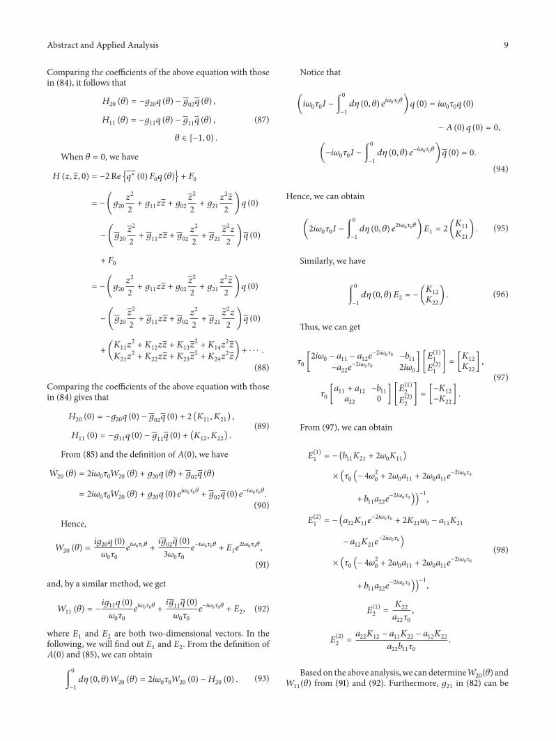
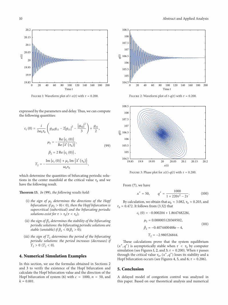
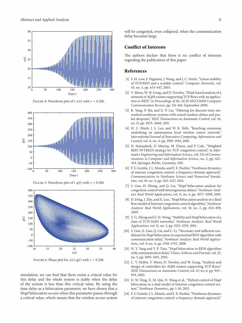
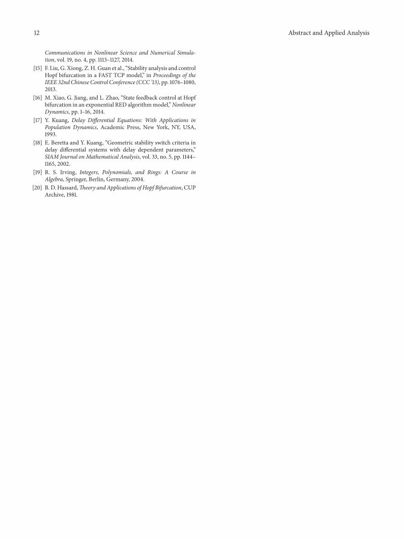