resampling in state space models - university of … · resampling in state space models∗ david...
TRANSCRIPT

Resampling in State Space Models∗
David S. Stoffer
Department of StatisticsUniversity of Pittsburgh
Pittsburgh, PA 15260 USA
Kent D. Wall
Defense Resources Management InstituteNaval Postgraduate SchoolMonterey, CA 93943 USA
Abstract. Resampling the innovations sequence of state space models has proved to be a useful tool in many
respects. For example, while under general conditions, the Gaussian MLEs of the parameters of a state space model
are asymptotically normal, several researchers have found that samples must be fairly large before asymptotic results
are applicable. Moreover, problems occur if the any of parameters are near the boundary of the parameter space. In
such situations, the bootstrap applied to the innovation sequence can provide an accurate assessment of the sampling
distributions of the parameter estimates. We have also found that a resampling procedure can provide insight into
the validity of the model. In addition, the bootstrap can be used to evaluate conditional forecast errors of state
space models. The key to this method is the derivation of a reverse-time innovations form of the state space model
for generating conditional data sets. We will provide some theoretical insight into our procedures that show why
resampling works in these situations, and we provide simulations and data examples that demonstrate our claims.
Key words. ARMAX models, Bootstrap, Finite sample distributions, Forecasting, Innovations filter, Kalman
filter, Reverse-time state space model, Stochastic regression, Stochastic volatility.
1 Introduction
A very general model that seems to subsume a whole class of special cases of interest is the statespace model or the dynamic linear model, which was introduced in Kalman (1960) and Kalmanand Bucy (1961). Although the model was originally developed as a method primarily for usein aerospace-related research, it has been applied to modeling data from such diverse fields aseconomics (e.g. Harrison and Stevens, 1976, Harvey and Pierse, 1984, Harvey and Todd, 1983,Kitagawa and Gersch 1984, Shumway and Stoffer, 1982), medicine (e.g. Jones, 1984) and molecularbiology (e.g. Stultz, et al, 1993). An excellent modern treatment of time series analysis based onthe state space model is the text by Durbin and Koopman (2001). We note, in particular, thatARMAX models can be written in state space form (see e.g. Shumway and Stoffer, 2000, §4.6), soanything we say and do here regarding state space models applies equally to ARMAX models.
Here, we write the state space model as
xxxt+1 = Φxxxt + Υuuut + wwwt t = 0, 1, ..., n (1)
yyyt = Atxxxt + Γuuut + vvvt t = 1, ..., n (2)
where xxxt represents the p-dimensional state vector, and yyyt represents the q-dimensional observationvector. In the state equation (1), the initial state xxx0 has mean µµµ0 and variance-covariance matrix
∗Chapter 9 of State Space and Unobserved Component Models: Theory and Applications, A. Harvey, S.J. Koopman
and N. Shephard (Eds). Cambridge University Press, 2004

Σ0; Φ is p× p, Υ is p× r, and uuut is an r× 1 vector of fixed inputs. In the observation equation (2),At is q × p and Γ is q × r. Here, wwwt and vvvt are white noise series (both independent of xxx0), withvar(wwwt) = Q, var(vvvt) = R, but we also allow the state noise and observation noise to be correlatedat time t; that is, cov(wwwt, vvvt) = S, and zero otherwise. Note, S is a p × q matrix. Throughout, weassume the model coefficients and the correlation structure of the model are uniquely parameterizedby a k × 1 parameter vector Θ; thus, Φ = Φ(Θ), Υ = Υ(Θ), Q = Q(Θ), At = At(Θ), Γ = Γ(Θ),R = R(Θ), and S = S(Θ).
We denote the best linear predictor of xxxt+1 given the data {yyy1, . . . , yyyt} as xxxtt+1, and denote the
covariance matrix of the prediction error, (xxxt+1 −xxxtt+1), as P t
t+1. The Kalman filter (e.g. Andersonand Moore, 1979) can be used to obtain the predictors and their covariance matrices successivelyas new observations become available. The innovation sequence, {εεεt; t = 1, . . . , n}, is defined tobe the sequence of errors in the best linear prediction of yyyt given the data {yyy1, . . . , yyyt−1}. Theinnovations are
εεεt = yyyt − Atxxxt−1t − Γuuut, t = 1, . . . , n, (3)
where the innovation variance-covariance matrix is given by
Σt = AtPt−1t A′
t + R, t = 1, . . . , n. (4)
The innovations form of the Kalman filter, for t = 1, . . . , n, is given by the following equationswith initial conditions xxx0
1 = Φµµµ0 + Υuuu0 and P 01 = ΦΣ0Φ′ + Q:
xxxtt+1 = Φxxxt−1
t + Υuuut + Ktεεεt, (5)
P tt+1 = ΦP t−1
t Φ′ + Q − KtΣtK′t, (6)
Kt = (ΦP t−1t A′
t + S)Σ−1t . (7)
In this article, we will work with the standardized innovations
eeet = Σ−1/2t εεεt, (8)
so we are guaranteed these innovations have, at least, the same first two moments. In (8), Σ1/2t
denotes the unique square root matrix of Σt defined by Σ1/2t Σ1/2
t = Σt. We now define the (p+q)×1vector
ξξξt =[xxxt
t+1
yyyt
].
Combining (3) and (5) results in a vector first-order equation for ξξξt given by
ξξξt = Ftξξξt−1 + Guuut + Hteeet, (9)
where
Ft =[
Φ 0At 0
], G =
[ΥΓ
], Ht =
[KtΣ
1/2t
Σ1/2t
].
Estimation of the model parameters Θ is accomplished by Gaussian quasi-maximum likelihood.The innovations form of the Gaussian likelihood (ignoring a constant) is
− lnLY (Θ) =12
n∑t=1
(ln |Σt(Θ)| + εεεt(Θ)′Σt(Θ)−1εεεt(Θ)
)
=12
n∑t=1
(ln |Σt(Θ)| + eeet(Θ)′eeet(Θ)
), (10)
1

where LY (Θ) denotes the likelihood of Θ given the data yyy1, . . . , yyyn assuming normality; note thatwe have emphasized the dependence of the innovations on the parameters Θ. We stress the fact thatit is not necessary for the data to be Gaussian to consider (10) as the criterion function to be usedfor parameter estimation. Furthermore, under certain rare conditions, the Gaussian quasi-MLEof Θ when the process is non-Gaussian is asymptotically optimal; details can be found in Caines(1988, Chapter 8).
2 Assessing the Finite Sample Distribution of Parameter
Estimates
Although, under general conditions (which we assume to hold in this section), the MLEs of theparameters of the model, Θ, are consistent and asymptotically normal, time series data are oftenof short or moderate length. Several researchers have found evidence that samples must be fairlylarge before asymptotic results are applicable (Dent and Min, 1978; Ansley and Newbold, 1980).Moreover, it is well known that problems occur if the parameters are near the boundary of theparameter space. In this section, we discuss an algorithm for bootstrapping state space models toassess the finite sample distribution of the model parameters. This algorithm and its justification,including the non-Gaussian case, along with examples and simulations, can be found in Stoffer andWall (1991).
Let Θ denote the Gaussian quasi-MLE of Θ, that is, Θ = argmaxΘLY (Θ), where LY (Θ) is givenin (10); of course, if the process is Gaussian, Θ is the MLE. Let εεεt(Θ) and Σt(Θ) be the innovationvalues obtained by running the filter under Θ. Once this has been done, the bootstrap procedureis accomplished by the following steps.
1. Construct the standardized innovations
eeet(Θ) = Σ−1/2t (Θ)εεεt(Θ).
2. Sample, with replacement, n times from the set {eee1(Θ), ..., eeen(Θ)} to obtain {eee∗1, ..., eee∗n}, abootstrap sample of standardized innovations.
3. To construct a bootstrap data set {yyy∗1, ..., yyy∗n}, solve (9) using eee∗t in place of eeet; that is, solve
ξξξ∗t = Ft(Θ)ξξξ∗t−1 + G(Θ)uuut + Ht(Θ)eee∗t , (11)
for t = 1, . . . , n. The exogenous variables uuut and the initial conditions of the Kalman filterremain fixed at their given values, and the parameter vector is held fixed at Θ. Note that abootstrapped observation yyy∗t is obtained from the final q rows of the (p + q) × 1 vector ξξξ∗t .Because of startup irregularities, it is sometimes a good idea to set yyy∗t ≡ yyyt for the first fewvalues of t, say t = 1, 2, . . . , t0, where t0 is small, and to sample from {eeet0+1(Θ), ..., eeen(Θ)}.That is, do not bootstrap the first few data points; typically setting t0 to 4 or 5 will suffice.
4. Using the bootstrap data set {yyy∗t ; t = 1, ..., n}, construct a likelihood, LY ∗(Θ), and obtainthe MLE of Θ, say, Θ∗.
2
5. Repeat steps 2 through 4, a large number, B, of times, obtaining a bootstrapped set ofparameter estimates {Θ∗
b ; b = 1, ..., B}. The finite sample distribution of (Θ − Θ) may beapproximated by the distribution of (Θ∗
b − Θ), for b = 1, ..., B.
2.1 Stochastic Regression
An interesting application of the state-space model was given in Newbold and Bos (1985, pp. 61-73).Of the several alternative models they investigate, we focus on the one specified by their equations(4.7a) and (4.7b). Their model has one output variable, the nominal interest rate recorded forthree-month treasury bills, yt. The output equation is specified by
yt = α + βtzt + vt,
where zt is the quarterly inflation rate in the Consumer Price Index, α is a fixed constant, βt is astochastic regression coefficient, and vt is white noise with variance σ2
v . The stochastic regressionterm, which comprises the state variable, is specified by a first-order autoregression,
(βt+1 − b) = φ(βt − b) + wt,
where b is a constant, and wt is white noise with variance σ2w. The noise processes, vt and wt, are
assumed to be uncorrelated.Using the notation of the state space model (1) and (2), we have in the state equation, xxxt = βt,
Φ = φ, uuut ≡ 1, Υ = (1 − φ)b, Q = σ2w, and in the observation equation, At = zt, Γ = α, R = σ2
v ,and S = 0. The parameter vector is Θ = (φ, α, b, σw , σv)′.
We consider the first estimation exercise reported in Table 4.3 of Newbold and Bos. This ex-ercise covers the period from the first quarter of 1953 through the second quarter of 1965, n = 50observations. We repeat their analysis so our results can be compared to their results. In addition,we focus on this analysis because it demonstrates that the bootstrap applied to the innovationsequence can provide an accurate assessment of the sampling distributions of the parameter esti-mates when analyzing short time series. Moreover, this analysis demonstrates that a resamplingprocedure can provide insight into the validity of the model.
The results of the Newton–Raphson estimation procedure are listed in Table 1. The MLEsobtained in Newbold and Bos are in agreement with our values, and differ only in the fourth decimalplace; the differences are attributed to the fact that we use a different numerical optimizationroutine. Included in Table 1 are the asymptotic standard errors reported in Newbold and Bos.Also shown in the Table 1 are the corresponding standard errors obtained from B = 500 runs ofthe bootstrap. These standard errors are simply the square root of
∑Bb=1(Θ
∗ib− Θi)2/(B−1), where
Θi, represents the ith parameter, i = 1, ..., 5, and Θi is the MLE of Θi.The asymptotic standard errors listed in Table 1 are typically smaller than those obtained from
the bootstrap. This result is the most pronounced in the estimates of φ, σw, and σv, where thebootstrapped standard errors are about 50% larger than the corresponding asymptotic value. Also,asymptotic theory prescribes the use of normal theory when dealing with the parameter estimates.The bootstrap, however, allows us to investigate the small sample distribution of the estimatorsand, hence, provides more insight into the data analysis.
For example, Figure 1 shows the bootstrap distribution of the estimator of φ. This distributionis highly skewed with values concentrated around 0.8, but with a long tail to the left. Some quantiles
3

Table 1: Comparison of Asymptotic Standard Errors (SE) andBootstrapped Standard Errors (B = 500).
Asymptotic Newbold & Bos BootstrapParameter MLE SE SE SE
φ 0.841 0.200 0.212 0.304α −0.771 0.645 0.603 0.645b 0.858 0.278 0.259 0.277
σw 0.127 0.092 na 0.182σv 1.131 0.142 na 0.217
Figure 1: Bootstrap distribution, B = 500, of the estimator of φ.
of the bootstrapped distribution of φ are −0.09 (2.5%), 0.03 (5%), 0.16 (10%), 0.87 (90%), 0.92(95%), 0.94 (97.5%), and they can be used to obtain confidence intervals. For example, a 90%confidence interval for φ would be approximated by (0.03, 0.92). This interval is rather wide, andwe will interpret this after we discuss the results of the estimation of σw.
Figure 2 shows the bootstrap distribution of the estimator of σw. The distribution is concen-trated at two locations, one at approximately σ∗
w = 0.15 and the other at σ∗w = 0. The cases in
which σ∗w ≈ 0 correspond to deterministic state dynamics. When σw = 0 and |φ| < 1, then βt ≈ b
for large t, so the approximately 25% of the cases in which σ∗w ≈ 0 suggest a fixed state, or con-
stant coefficient model. The cases in which σ∗w is away from zero would suggest a truly stochastic
regression parameter. To investigate this matter further, Figure 3 shows the joint bootstrapped es-timates, (φ∗, σ∗
w), for non-negative values of φ∗. The joint distribution suggests σ∗w > 0 corresponds
to φ∗ ≈ 0. When φ = 0, the state dynamics are given by βt = b + wt. If, in addition, σw is small
4

Figure 2: Bootstrap distribution, B = 500, of the estimator of σw.
o
o
o
o
oo
o
o
o
o
o
o
o
o
o
o
o
o
o
o
o
o
o
o
o
o
o
oo
o
o
o
o
o
o
o
o
o
o
o
o
o
o
o
o
o
o o
o
o
o
o
o
oo
o
o
o
o
o
oo
o
o
o
o
o
o
o
o
o
o
o
o
o
o
o
o
o
o
o
o
o
o
o
o
o
o
oo
o
oo
o
o
o
o
o
oo
o
o
o
oo
oo
o
o
o
o
o
o
o
o
o
o
o
o
o
o
o
o
o
oo oo o
o
o o
o oo
o
o
o
o
o
o
o
o
o
oo
o
o
o
o
o
o
oo
o
o
o
o
o
o
o
o
oo
o
o
o
o
o
o
o
o
o
o
o
o
o
o
o
o
o
o
o
o
o
o
o
o
o
o
o
o
o
o
o
o
o
o
o
o
o
o
o
o
o
oo
o
o
o
o
oo
o
o
o
o
o
o
o
o
o
o
o
o
o
o
o
o
o
o
o
o
o
o
o
oo
o
o
o o
o
o
o
o
o oo
o
o
o
o
oo
o
o
o
o
o
o
o
o
o
oo
o
o
o
o
o
o
o
o
o
o o
o
o
o
o
o
o
o
o
o
o
o
o
o
o
o
o
o
o
oo
o
o
o
o
o
oo
o
o
o
o
o
o
o
o
o
o
o
o
o
o
o
o
o
o
o
o
o
o
o
o
o
o
o
o
oo
o
o
o
o
o
o
o
o
o
o
o
o
o
o
oo
o
o
o
o
o
o
o
o
o
o
o
o
o
oo
o
o
o
o
o
o
oo o
o
o
o
o
o o
o
oo
o o
o
o
o
o
o
o
o
o
o
o
o
o
o
o
o
o
o
o
o
o
o
o
o
oo
o
o o
o
o
o
o
o
o
o
o
o
o
o
o
o
o
o
o
oo
o
o
o
o
o
o
o
oo
o
o
o
o
o
o
o
oo o
o
o
o
o
o
o
o
o
o
o
o
o
o
oo
o o
o
o
o
ooo
o
o
o
o
o
o
o
o
o
o
o
o
o
o
o
o
o
o
o
o
o
o
o
o
o
o o
phi
sigma
0.0 0.2 0.4 0.6 0.8 1.0
0.00.1
0.20.3
0.40.5
Figure 3: Joint bootstrap distribution, B = 500, of the estimators of φ and σw. Only the valuescorresponding to φ∗ ≥ 0 are shown.
relative to b (as it appears to be in this case), the system is nearly deterministic; that is, βt ≈ b.Considering these results, the bootstrap analysis leads us to conclude the dynamics of the data arebest described in terms of a fixed, rather than stochastic, regression effect.
5

If, however, we use the same model for the entire data set presented in Newbold and Bos(that is, 110 quarters of three-month treasury bills and inflation rate, covering 1953:I to 1980:II),stochastic regression appears to be appropriate. In this case the estimates using Newton-Raphsonwith estimated standard errors (“asymptotic” | “bootstrap”) are:
φ = 0.896 (0.067 | 0.274), α = −0.970 (0.475 | 0.538), b = 1.090 (0.158 | 0.221),
σw = 0.117 (0.037 | 0.122), σv = 1.191 (0.108 | 0.171).
We note that the asymptotic standard error estimates are still too small, and the bootstrappeddistribution of φ is still markedly skewed. In particular, a 90% bootstrap confidence interval for φ
is (.46, .92).
2.2 Stochastic Volatility
This problem is somewhat different than the previous section in that it is not a straight-forwardapplication of the algorithm. In this example, we consider the stochastic volatility model due toHarvey, Ruiz and Shephard (1994). Let rt denote the return or growth rate of a process of interest.For example, if st is the value of a stock at time t, the return or relative gain of the stock isrt = ln(st/st−1). Typically, it is var(rt) = σ2
t that is of interest. In the stochastic volatility model,we model ht = ln σ2
t as an AR(1), that is,
ht+1 = φ0 + φ1ht + wt, (12)
where wt is white Gaussian noise with variance σ2w; this comprises the state equation. The obser-
vations are taken to be yt = ln r2t , and yt is related to the state via
yt = α + ht + vt. (13)
Together, (12) and (13) make up the stochastic volatility model, where ht represents the unob-served volatility of the process yt. If vt was Gaussian white noise, (12)–(13) would form a Gaussianstate space model, and we could then use standard results to fit the model to data. Unfortunately,yt = ln r2
t is rarely normal, so one typically assumes that vt = ln z2t where zt is standard Gaussian
white noise. In this case, ln z2t is distributed as the log of a chi-squared random variable with one
degree of freedom. Kim, Shephard and Chib (1998) proposed modeling the log of a chi-squaredrandom variable by a mixture of normals.
Various approaches to the fitting of stochastic volatility models have been examined; thesemethods include a wide range of assumptions on the observational noise process. A good summaryof the proposed techniques, both Bayesian (via MCMC) and non-Bayesian approaches (such asquasi-maximum likelihood estimation and the EM algorithm), can be found in Jacquier et al (1994),and Shephard (1996). Simulation methods for classical inference applied to stochastic volatilitymodels are discussed in Danielson (1994) and Sandmann and Koopman (1998).
In an effort to keep matters simple, our method (see Shumway and Stoffer, 2000, §4.10) of fittingstochastic volatility models is to retain the Gaussian state equation (12), but in the observationequation (13), we consider vt to be white noise, and distributed as a mixture of two normals, onecentered at zero. In particular, we write
vt = (1 − ηt)zt0 + ηtzt1, (14)
6

where ηt is an iid Bernoulli process, Pr{ηt = 0} = π0, Pr{ηt = 1} = π1, with π0 + π1 = 1, andwhere zt0 ∼ iid N(0, σ2
0), and zt1 ∼ iid N(µ1, σ21).
The advantage of this model is that it is fairly easy to fit because it uses normality. The modelspecified by equations (12)–(14), and the corresponding filter, are similar to those presented inPena and Guttman (1988), who used the idea to obtain a robust Kalman filter, and, as previouslymentioned, Kim, Shephard and Chib (1998). In addition, this technique is similar to techniquediscussed in Shumway and Stoffer (2000, §4.8). In particular, the filtering equations for this modelare:
htt+1 = φ0 + φ1h
t−1t +
1∑j=0
πtjKtjεtj , (15)
P tt+1 = φ2
1Pt−1t + σ2
w −1∑
j=0
πtjK2tjΣtj , (16)
εt0 = yt − α − ht−1t , (17)
εt1 = yt − α − ht−1t − µ1, (18)
Σt0 = P t−1t + σ2
0 , (19)
Σt1 = P t−1t + σ2
1 , (20)
Kt0 = φ1Pt−1t / Σt0, (21)
Kt1 = φ1Pt−1t / Σt1. (22)
To complete the filtering, we must be able to assess the probabilities πt1 = Pr(ηt = 1 | y1, . . . , yt),for t = 1, . . . , n; of course, πt0 = 1− πt1. Let fj(t | t− 1) denote the conditional density of yt giventhe past y1, ..., yt−1, and ηt = j (j = 0, 1). Then,
πt1 =π1f1(t | t − 1)
π0f0(t | t − 1) + π1f1(t | t − 1), (23)
where we assume the distribution πj, for j = 0, 1 has been specified a priori. If the investigatorhas no reason to prefer one state over another the choice of uniform priors, π1 = 1/2, will suffice.Unfortunately, it is computationally difficult to obtain the exact values of fj(t | t− 1); although wecan give an explicit expression of fj(t | t − 1), the actual computation of the conditional density isprohibitive. A viable approximation, however, is to choose fj(t | t − 1) to be the normal density,N(ht−1
t + µj, Σtj), for j = 0, 1 and µ0 = 0; see Shumway and Stoffer (2000, §4.8) for details.The innovations filter given in (15)–(23) can be derived from the Kalman filter by a simple
conditioning argument. For example, to derive (15), we write
E (ht+1 | y1, . . . , yt) =1∑
j=0
E (ht+1 | y1, . . . , yt, ηt = j) Pr(ηt = j | y1, . . . , yt)
=1∑
j=0
(φ0 + φ1h
t−1t + Ktjεtj
)πtj
= φ0 + φ1ht−1t +
1∑j=0
πtjKtjεtj .
7

Estimation of the parameters, Θ = (φ0, φ1, σ20 , µ1, σ
21 , σ
2w)′, is accomplished via MLE based on
the likelihood given by
ln LY (Θ) =n∑
t=1
ln
⎛⎝ 1∑
j=0
πj fj(t | t − 1)
⎞⎠ , (24)
where the densities for fj(t | t−1) are approximated by the normal densities previously mentioned.To perform the bootstrap, we develop a vector first-order equation, as was done in (9). First,
using (17)–(18), and noting that yt = πt0yt + πt1yt, we may write
yt = α + ht−1t + πt0εt0 + πt1(εt1 + µ1). (25)
Consider the standardized innovations
etj = Σ−1/2tj εtj , j = 0, 1, (26)
and define the 2 × 1 vector
eeet =[et0
et1
].
Also, define the 2 × 1 vector
ξξξt =[ht
t+1
yt
].
Combining (15) and (25) results in a vector first-order equation for ξξξt given by
ξξξt = Fξξξt−1 + Gt + Hteeet, (27)
where
F =[φ1 01 0
], Gt =
[φ0
α + πt1µ1
], Ht =
[πt0Kt0Σ
1/2t0 πt1Kt1Σ
1/2t1
πt0Σ1/2t0 πt1Σ
1/2t1
].
Hence, the steps in bootstrapping for this case are the same as steps 1 through 5 previouslydescribed, but with (11) replaced by the following first-order equation:
ξξξ∗t = F (Θ)ξξξ∗t−1 + Gt(Θ; πt1) + Ht(Θ; πt1)eee∗t , (28)
where Θ = (φ0, φ1, σ20 , α, µ1, σ
21 , σ
2w)′ is the MLE of Θ, and πt1 is estimated via (23), replacing
f1(t | t − 1) and f0(t | t − 1) by their respective estimated normal densities (πt0 = 1 − πt1).To examine the efficacy of the bootstrap for the stochastic volatility model, we generated n = 200
observations from the following stochastic volatility model:
ht = .95ht−1 + wt, (29)
where wt is white Gaussian noise with variance σ2w = 1. The observations were then generated as
yt = ht + vt, (30)
where the observational white noise process, vt, is distributed as the log of a chi-squared randomvariable with one degree of freedom. The density of vt is given by
fv(x) =1√2π
exp{−1
2(ex − x)
}−∞ < x < ∞, (31)
8

Figure 4: Simulated data, n = 200, from the stochastic volatility model (29)–(30).
and its mean and variance are −1.27 and π2/2, respectively; the density (31) is highly skewedwith a long tail on the left. The data are shown in Figure 4. Then, we assumed the true errordistribution was unknown to us, and we fit the model (12)–(14) using the Gauss BFGS variablemetric algorithm to maximize the likelihood. The results for the state parameters are given in Table2 in the columns marked MLE and Asymptotic SE. Next, we bootstrapped the data, B = 500 times,using the incorrect model (12)–(14) to assess the finite sample standard errors (SE). The results arelisted in Table 2 in the column marked Bootstrap SE. Finally, using the correct model, (29)–(30), wesimulated 500 processes, estimated the parameters based on the model (12)–(14) also via a BFGSvariable metric algorithm, and assessed the SEs of the estimates of the actual state parameters.These values are listed in Table 2 in the column labeled “True” SE.
Table 2: Stochastic Volatility Simulation Results.State Actual Asymptotic Bootstrap “True”
Parameter Value MLE SE SE† SE‡φ 0.95 0.963 0.032 0.032 0.036σw 1 1.042 0.279 0.215 0.252
† Based on 500 bootstrapped samples. ‡ Based on 500 replications.
In Table 2 we notice that the bootstap SE and the asymptotic SE of φ are about the same; also,both estimates are slightly smaller than the “true” value. The interest here, however, is not so muchin the SEs, but in the actual sampling distribution of the estimates. To explore the finite sampledistribution of the estimate of φ, Figure 5 shows the centered bootstrap histogram: (φ∗
b − φ), forb = 1, . . . , 500 bootstrapped replications [the bars are filled with lines of positive slope], the centered
9

“true” histogram: (φj − φ), where φj is the MLE obtained on the j-th iteration, for j = 1, . . . , 500Monte Carlo replications [the bars are filled with flat lines], and the centered asymptotic normaldistribution of (φ − φ) [appropriately scaled for comparison with the histograms], superimposedon eachother. Clearly, the bootstrap distribution is closer to the “true” distribution than theestimated asymptotic normal distribution; the bootstrap distribution captures the positive kurtosis(peakedness) and asymmetry of the “true” distribution.
Figure 5: Sampling distributions of the estimate of φ; simulated data example: The centeredbootstrap histogram (lines with positive slope), the centered “true” histogram (flat lines), and thecentered asymptotic normal distribution.
In an example using actual data, we consider the analysis of quarterly U.S. GNP from 1947(1)to 2002(3), n = 223. The data are seasonally adjusted and were obtained from the Federal ReserveBank of St. Louis (http://research.stlouisfed.org/fred/data/gdp/gnpc96). The growth rateis plotted in Figure 6 and appears to be a stable process. Analysis of the data indicates the growthrate is an MA(2) [for more details of this part of the analysis, see Shumway and Stoffer, 2000, §2.8],however, the residuals of that fit, which appear to be white, suggest that there is volatility.
Figure 7 shows the log of the squared residuals, say yt, from the MA(2) fit on the U.S. GNPseries. The stochastic volatility model (12)–(14) was then fit to yt. Table 3 shows the MLEs of themodel parameters along with their asymptotic SEs assuming the model is correct. Also displayed inTable 3 are the means and SEs of B = 500 bootstrapped samples. As in the simulation, there is someamount of agreement between the asymptotic values and the bootstrapped values. Based on theprevious simulation, we would be more prone to focus on the actual sampling distributions, ratherthan assume normality. For example, Figure 8 compares the bootstrap histogram and asymptotic
10

Figure 6: U.S. GNP quarterly growth rate.
Figure 7: Log of the squared residuals from an MA(2) fit on GNP growth rate.
normal distribution of φ1. In this case, as in the simulation, the bootstrap distribution exhibitspositive kurtosis and skewness which is missed by the assumption of asymptotic normality. Basedon the simulation, we would be prone to believe the results of the bootstrap are fairly accurate.
11

Figure 8: Bootstrap histogram and asymptotic distribution of φ1 for the US GNP example.
Table 3: Estimates and Their Asymptotic and BootstrapStandard Errors for US GNP Example.
Asymptotic Bootstrap BootstrapParameter MLE SE Mean† SE†
φ0 0.068 0.274 −0.010 0.353φ1 0.900 0.099 0.864 0.102σw 0.378 0.208 0.696 0.375α −10.524 2.321 −10.792 0.748µ1 −2.164 0.567 −1.941 0.416σ1 3.007 0.377 2.891 0.422σ0 0.935 0.198 0.692 0.362
† Based on 500 bootstrapped samples.
3 Assessing the Finite Sample Distribution of Conditional
Forecasts
In this section we focus on assessing the conditional forecast accuracy of time series models using astate space approach and resampling methods. Our work is motivated by the following considera-tions. First, the state space model provides a convenient unifying representation for various models,including ARMA(p, q) models. Second, the actual practice of forecasting involves the predictionof a future point based on an observed sample path, thus conditional forecast error assessmentis of most interest. Third, real-life applications involving time series data are often characterizedby short data sets and lack of distributional information. Asymptotic theory provides little help
12

here and often there are no compelling reasons to assume Gaussian distributions apply. Finally,the utility and applicability already demonstrated by the bootstrap for prediction of AR processessuggests that it has much to offer in the prediction of other processes.
Early application of the bootstrap to assess conditional forecast errors can be found in Find-ley (1986), Stine (1987), Thombs and Schuchany (1990), Kabaila (1993) and McCullough (1994,1996). Interest in the evaluation of confidence intervals for conditional forecast errors has led tomethodological problems because a backward, or reverse-time, set of residuals must be generated.Findley (1986) first discussed this problem and Breidt, Davis and Dunsmuir (1992, 1995) offereda solution that is implemented in the work of McCullough (1994, 1996). To date there is a wellgrounded methodology for AR models and this work has established the utility of the bootstrap.
A similar state of affairs appears not to exist for other time series models. We suspect this isdue to the difficulty with which one can identify mechanisms required to generate bootstrap datasets, whether forwards or backwards in time. For AR models this is easily accomplished becausethe required initial, or terminal (in the case of conditional forecasts), conditions are given in termsof the observed series. With other time series models this may not be the case because the modelsrequire solutions of difference equations involving unobserved disturbances.
The state space model and its related innovations filter offer a way around this difficulty. It isworthwhile, therefore, to investigate how well this can be done in practice. In §2, such a combinationwas of use in assessing parameter estimation error, and this naturally leads to the same questionbeing asked in relation to conditional prediction errors. We find that the bootstrap is as usefulin evaluating conditional forecast errors as it has proven to be in assessing parameter estimationerrors, particularly in a non-Gaussian environment. Our presentation is based on the work of Walland Stoffer (2002).
3.1 Generating Reverse Time Datasets
As seen in §2, the generation of bootstrap data sets in forward time is easy. Given an initialcondition or prior, (11) is solved recursively for t = 1, . . . , n to produce realizations passing throughthe given initial condition. Such computations are all that is required in obtaining bootstrapestimates of parameter estimation error statistics or unconditional forecast error statistics. Thegeneration of bootstrap data sets for assessing conditional forecast errors is not so straight forwardbecause they must be generated backward and this requires a backward-time state space model.
An early discussion of the problems related to backward time models in assessing conditionalforecast errors is found in Findley (1986). Further consideration of the problem is found in Breidt,Davis and Dunsmuir (1992, 1995). This literature stresses the need to properly construct a set of“backward” residuals and Breidt, Davis and Dunsmuir (1992, 1995) provide an algorithm for thisthat solves the problem for AR(p) models. A similar result is needed for state space models, butdevelopment of backward-time representations has not received much attention in the literature.Notable exceptions are the elegant presentation found in Caines (1988, Ch 4) and a derivation inAoki (1989, Ch 5). Our work requires an extension of their results to the time-varying case.
The key system in generating bootstrap data sets is the innovations filter form, (9); recall
ξξξt = Ftξξξt−1 + Guuut + Hteeet, (9)
13

whereξξξt =
[xxxt
t+1
yyyt
], Ft =
[Φ 0At 0
], G =
[ΥΓ
], Ht =
[KtΣ
1/2t
Σ1/2t
].
We require a backward-time representation of this system. All the problems highlighted by Findley(1986) and Breidt, Davis and Dunsmuir (1992, 1995) appear here. For example, the first p rows of(9) cannot be solved backwards in time by simply expressing xxxt−1
t in terms of xxxtt+1. First, Φ is not
always invertible; e.g., MA(q) models. Second, even when Φ is invertible, Φ−1 has characteristicroots outside the unit circle whenever Φ has its characteristic roots inside the unit circle. Thissituation is intolerable in generating reverse time trajectories because of the explosive nature of thesolutions for ξξξt. In addition, we now have a time-varying system.
These difficulties are overcome by building on the method found in Caines (1988, pp. 236-237).Special attention must be given to the way in which the time-varying matrices propagate throughthe derivations and proper account must be taken of the effects of the known, or observed inputsequence uuut. For ease, we will assume here that uuut ≡ 000; the general case is presented in Wall andStoffer (2002). Application of the symmetry of minimal splitting subspaces yields the followingreverse-time state space representation for t = n − 1, n − 2, . . . , 1:
rrrt = Φ′rrrt+1 + Btxxxt−1t − Cteeet
yyyt = Ntrrrt+1 − Ltxxxt−1t + Mteeet
where
Bt = V −1t − Φ′V −1
t+1Φ
Ct = Φ′V −1t+1KtΣ
−1/2t ,
Dt = I − Σ−1/2t K ′
tV−1t+1KtΣ
−1/2t ,
Lt = Σ−1/2t C ′
t − AtVtBt,
Mt = Σ−1/2t Dt − AtVtCt,
Nt = AtVtΦ′ + Σ−1t K ′
t,
andVt+1 = ΦVtΦ′ + KtΣ−1
t K ′t.
The reverse-time state vector is rrrt. The backward recursion is initialized by rrrn = V −1n xxxn−1
n . Detailsof the derivation are given in Wall and Stoffer (2002).
The above recursion specifies a three step procedure for the generation of backward time datasets (written here for uuut ≡ 0):
1. Generate Vt, Bt, Ct,Dt, Lt,Mt and Nt forwards in time, t = 1, . . . , n, with initial condition
V1 = P 01 (32)
2. For given {eee∗t ; 1 ≤ t ≤ n − 1}, set xxx∗1 = 0 and generate {xxx∗
t ; 1 ≤ t ≤ n} forwards in time,t = 1, . . . , n, via
xxx∗t+1 = Φxxx∗
t + KtΣ1/2t eee∗t (33)
14
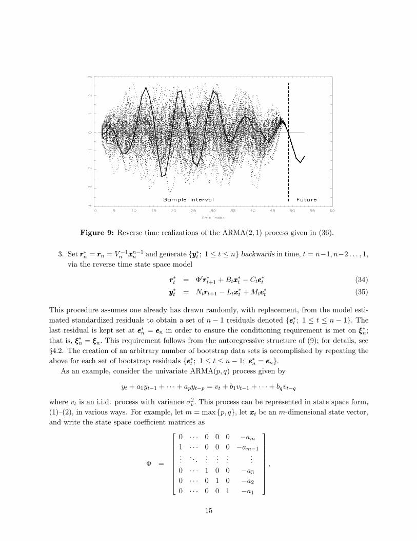
Figure 9: Reverse time realizations of the ARMA(2, 1) process given in (36).
3. Set rrr∗n = rrrn = V −1n xxxn−1
n and generate {yyy∗t ; 1 ≤ t ≤ n} backwards in time, t = n−1, n−2 . . . , 1,via the reverse time state space model
rrr∗t = Φ′rrr∗t+1 + Btxxx∗t − Cteee
∗t (34)
yyy∗t = Ntrrrt+1 − Ltxxx∗t + Mteee
∗t (35)
This procedure assumes one already has drawn randomly, with replacement, from the model esti-mated standardized residuals to obtain a set of n − 1 residuals denoted {eee∗t ; 1 ≤ t ≤ n − 1}. Thelast residual is kept set at eee∗n = eeen in order to ensure the conditioning requirement is met on ξξξ∗n;that is, ξξξ∗n = ξξξn. This requirement follows from the autoregressive structure of (9); for details, see§4.2. The creation of an arbitrary number of bootstrap data sets is accomplished by repeating theabove for each set of bootstrap residuals {eee∗t ; 1 ≤ t ≤ n − 1; eee∗n = eeen}.
As an example, consider the univariate ARMA(p, q) process given by
yt + a1yt−1 + · · · + apyt−p = vt + b1vt−1 + · · · + bqvt−q
where vt is an i.i.d. process with variance σ2v . This process can be represented in state space form,
(1)–(2), in various ways. For example, let m = max {p, q}, let xxxt be an m-dimensional state vector,and write the state space coefficient matrices as
Φ =
⎡⎢⎢⎢⎢⎢⎢⎢⎢⎢⎣
0 · · · 0 0 0 −am
1 · · · 0 0 0 −am−1...
. . ....
......
...0 · · · 1 0 0 −a3
0 · · · 0 1 0 −a2
0 · · · 0 0 1 −a1
⎤⎥⎥⎥⎥⎥⎥⎥⎥⎥⎦
,
15
A =[
0 · · · 0 0 0 1],
Υ = 0 and Γ = 0. The state noise process is defined by the wwwt = ggg vt where
ggg =[
bm − am, bm−1 − am−1, · · · b3 − a3, b2 − a2, b1 − a1
]′.
If m > p then a� = 0 for > p, and if m > q then b� = 0 for > q. The variance-covariance matricesare given by
Q = σ2v ggg ggg′, R = σ2
v , S = σ2v ggg.
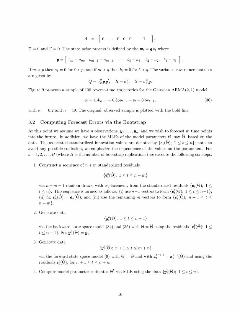
Figure 9 presents a sample of 100 reverse-time trajectories for the Gaussian ARMA(2, 1) model
yt = 1.4yt−1 − 0.85yt−2 + vt + 0.6vt−1, (36)
with σv = 0.2 and n = 49. The original, observed sample is plotted with the bold line.
3.2 Computing Forecast Errors via the Bootstrap
At this point we assume we have n observations, yyy1, . . . , yyyn, and we wish to forecast m time pointsinto the future. In addition, we have the MLEs of the model parameters Θ, say Θ, based on thedata. The associated standardized innovation values are denoted by {eeet(Θ); 1 ≤ t ≤ n}; note, toavoid any possible confusion, we emphasize the dependence of the values on the parameters. Forb = 1, 2, . . . , B (where B is the number of bootstrap replications) we execute the following six steps:
1. Construct a sequence of n + m standardized residuals
{eeebt(Θ); 1 ≤ t ≤ n + m}
via n + m− 1 random draws, with replacement, from the standardized residuals {eeet(Θ); 1 ≤t ≤ n}. This sequence is formed as follows: (i) use n−1 vectors to form {eeeb
t(Θ); 1 ≤ t ≤ n−1};(ii) fix eeeb
n(Θ) = eeen(Θ); and (iii) use the remaining m vectors to form {eeebt(Θ); n + 1 ≤ t ≤
n + m}.
2. Generate data{yyyb
t(Θ); 1 ≤ t ≤ n − 1}via the backward state space model (34) and (35) with Θ = Θ using the residuals {eeeb
t(Θ); 1 ≤t ≤ n − 1}. Set yyyb
n(Θ) = yyyn.
3. Generate data{yyyb
t(Θ); n + 1 ≤ t ≤ m + n}via the forward state space model (9) with Θ = Θ and with xxxt−1;b
t = xxxt−1t (Θ) and using the
residuals eeebt(Θ), for n + 1 ≤ t ≤ n + m.
4. Compute model parameter estimates Θb via MLE using the data {yyybt(Θ); 1 ≤ t ≤ n}.
16

5. Compute the bootstrap conditional forecasts
{yyybt(Θ
b); n + 1 ≤ t ≤ m + n}
via the forward time state space model (9) with Θ = Θb, and with xxxt−1;bt = xxxt−1
t (Θb) andeeeb
t = 0 for n + 1 ≤ t ≤ n + m.
6. Compute the bootstrap conditional forecast errors via:
δδδb� = yyyb
n+�(Θ) − yyybn+�(Θ
b); 1 ≤ ≤ m.
The extent to which the bootstrap captures the behavior of the actual forecast errors derivesfrom the extent to which these errors mimic the stochastic process δδδ� = yyyn+�(Θ) − yyyn+�(Θ); 1 ≤ ≤ m.
As an example, consider the univariate ARMA(1, 1) process given by
yt = 0.7yt−1 + vt + 0.10vt−1 (37)
where vt = 0.2zt and zt is a mixture of 90% N(µ = −1/9, σ = .15) and 10% N(µ = 1, σ = .15). Todemonstrate the benefits of resampling, we will assume that we do not know the true distributionof vt and will act as if it was normal. The model is first-order with
Φ = [0.70] A = [1] and ggg = [0.80] ,
in the notation of previous example.In this simulation we use B = 2, 000 and m = 4. The approximate “true” distribution is then
given by the relative frequency histogram of the observed conditional forecast errors. The resultsof the simulation is summarized by two sets of four histograms. One set (Figure 10) presents theapproximate “true” relative frequency histograms for each forecast lead time, while the other set(Figure 11) presents the relative frequency histograms obtained from application of the bootstrap.Superimposed on each is the Gaussian density that follows from application of the asymptoticGaussian theory. The simulation uses a short data set with n = 49 to emphasize the efficacy ofthe bootstrap when the use asymptotics is questionable and where bias is a factor in the forecasts.Prediction intervals follow immediately from the data summarized in the histograms. Althoughwe choose to present only the histograms, the percentile, the bias-corrected (BC), and the accel-erated bias-corrected (BCa) method all are applicable for generating confidence intervals using thegenerated data (see Efron, 1987).
Figures 10 and 11 reveal the value of the bootstrap. Indication of the mixture distribution isstriking in both the “true” and the bootstrap; the bimodality and asymmetry are clearly evident.
3.3 Stochastic Regression
We now illustrate the use of the bootstrap in assessing forecast errors in the data set analyzed in§2.1. Recall, the treasury bill interest rate is modeled as being linearly related to quarterly inflationas
yt = α + βtzt + vt,
17

Figure 10: “True” forecast histograms for the ARMA(1, 1) process given in (37).
Figure 11: Bootstrap forecast histograms for the ARMA(1, 1) process given in (37).
where α is a fixed constant, βt is a stochastic regression coefficient, and vt is white noise withvariance σ2
v . The stochastic regression term, which comprises the state variable, is specified by afirst-order autoregression,
(βt − b) = φ(βt−1 − b) + wt,
18

Figure 12: Dymanic behavior of the quantiles of ybn+�(Θ) [upper left panel], the quantiles of
ybn+�(Θ
b) [upper right panel], and the quantiles of the bootstrap conditional forecast errors ybn+�(Θ)−
ybn+�(Θ
b), for = 1, 2, 3, 4 [lower left panel]. The yt series [lower right panel] as a bold line andthe envelope of the backward data series as fine lines above and below the observed sample in thestochastic regression example.
where b is a constant, and wt is white noise with variance σ2w. The noise processes, vt and wt, are
assumed to be uncorrelated.The model parameter vector contains five elements, Θ = (φ, α, b, σw , σv)′ and is estimated via
Gaussian quasi-maximum likelihood using data from the first quarter of 1967 through the secondquarter of 1979 (49 observations). The MLEs and their estimated standard errors (in parentheses)were:
φ = 0.898 (0.101) α = −0.615 (1.457) b = 1.195 (0.278)
σw = 0.092 (0.049) σv = 1.287 (0.197)
Among the many forecast error assessment questions that can be asked concerning this modelare ones concerning the properties of the conditional forecast error distribution assuming that we
know the future values of the inflation rate. In particular, is a Gaussian assumption warrantedwhen assume we know the actual future values of zt? Such questions may arise within the contextof a “rational expectations” framework wherein economic agents are assumed so well informed thatthey “know” the inflation rate. The bootstrap, coupled with our methodology here, can shed somelight on just such a question as this.
Figure 12 depicts the bootstrap results with B = 2000. The upper left panel presents thedynamic behavior of the quantiles (specifically, 2.5%, 5%, 16%, 50%, 84%, 95%, 97.5%) of yb
n+�(Θ)and the upper right panel presents the quantiles of yb
n+�(Θb). Given the significant variability in
the upper right panel, it is clear that the variability due to the additive disturbances (upper left
19

Figure 13: Histograms of four conditional forecast errors, B = 2000, in the stochastic regressionexample.
Figure 14: Histograms of four conditional forecast errors, B = 10, 000, in the stochastic regressionexample.
panel) is not the dominant factor in the forecast uncertainty that it is so often assumed to be. Thelower left panel the depicts dynamic behavior of the quantiles of the bootstrap conditional forecasterrors yb
n+�(Θ)− ybn+�(Θ
b), for = 1, 2, 3, 4. The lower right panel plots the yt series as a bold line
20

and the envelope of the backward data series as fine lines above and below the observed sample.We find the backward generated series to be highly representative of the stochastic properties ofthe observed series.
Figure 13 presents histograms of the conditional forecast errors, ybn+�(Θ) − yb
n+�(Θb), for =
1, 2, 3, 4, when B = 2000 and Figure 14 presents the histograms when B = 10, 000. Each pic-ture gives indication of the problems in assuming that the asymptotic theory applies. Negativebias is indicated and t-tests reject zero means for = 2, 3, 4, in both bootstrap experiments. AKolmogorov-Smirnov test rejects the asymptotic Gaussian distribution (which are also displayed inthe figures) for all forecast lead times for both values of B. It appears little is gained in extendingthe bootstrap replications beyond B = 2000, other than the more “smooth” appearance of thehistograms.
4 Discussion
The state space model provides a convenient unifying representation for various time domain mod-els. This article demonstrates the utility of resampling the innovations of time domain models viastate space models and the Kalman (innovations) filter. We have based our presentation primarilyon the material in two articles, Stoffer and Wall (1991) and Wall and Stoffer (2002).
In Stoffer and Wall (1991) we developed a resampling scheme to assess the finite sample distri-bution of parameter estimates for general time domain models. This algorithm uses the eleganceof the state space model in innovations form to construct a simple resampling scheme. The keypoint is that while under general conditions, the MLEs of the model parameters are consistent andasymptotically normal, time series data are often of short or moderate length so that the use ofasymptotics may lead to wrong conclusions. Moreover, it is well known that problems occur if theparameters are near the boundary of the parameter space. We have provided additional exampleshere that emphasize the usefulness of the algorithm. We have also explained, heuristically, why theresampling scheme is asymptotically correct under appropriate conditions.
We have also discussed conditional forecast accuracy of time domain models using a state spaceapproach and resampling methods that was first presented in Wall and Stoffer (2002). Applicationsinvolving time series data are often characterized by short data sets and lack of distributionalinformation; asymptotic theory provides little help here and frequently there are no compellingreasons to assume Gaussian distributions apply. Interest in the evaluation of confidence intervalsfor conditional forecast errors in AR models led to methodological problems because a backward,or reverse-time, set of residuals must be generated. This problem was eventually solved and there isnow a well grounded methodology for AR models. Researchers were confined to AR models becausethe required initial, or terminal (in the case of conditional forecasts), conditions are given in termsof the observed series. With other time series models this may not be the case because the modelsrequire solutions of difference equations involving unobserved disturbances. The state space modeland its related innovations filter offered a way around this difficulty. We have exhibited a reverse-time state space in innovations form. We have presented additional examples here that demonstrateresampling as useful in evaluating conditional forecast errors as it has proven to be in assessingparameter estimation errors, particularly in a non-Gaussian environment. In the Appendix, weexplain, heuristically, why resampling works in large samples.
21

Appendix: Large Sample Heuristics
In §2, resampling techniques were used to determine the finite sample distributions of the parameter esti-mates when the use of asymptotics was questionable. In §3, we used resampling to assess the finite sampledistributions of the forecast errors. The extent to which resampling the innovations does what it is supposedto do can be measured in various ways. In the finite sample case, we can perform simulations—where thetrue distributions are known—and compare the bootstrap results to the known results. If the bootstrapworks well in simulations, we may feel confident that the bootstrap will work well in similar situations,but, of course, we have no guarantee that it works in general. In this way, the examples in §2 and §3 helpdemonstrate the validity of the resampling procedures discussed in those sections.
Another approach is to ask if the bootstrap will give the correct asymptotic answer. That is, if we havean infinite amount of data and can resample an infinite amount of times, do we get the correct asymptoticdistribution (typically, we require asymptotic normality). If the answer is no, we can assume that resamplingwill not work with small samples. If the answer is yes, we can only hope that resampling will work withsmall samples, but again, we have no guarantee. For state space models, how well the resampling techniquesperform in finite samples hinges on at least three things. First, the techniques are conditional on the data,so the success of the resampling depends on how typical the data set is for the particular model. Second, weassume the model is correct (at least approximately); if the proposed model is far from the truth, the resultsof the resampling will also be incorrect. Finally, assuming the data set is typical and the model is correct,the success of the resampling depends on how close the empirical distribution of the innovations is to theactual distribution of the innovations. We are guaranteed such closeness in large samples if the innovationsare stable and mixing in the sense of Gastwirth and Rubin (1975).
Section 2 Heuristics
Stoffer and Wall (1991) established the asymptotic justification of the procedure presented in §2 undergeneral conditions (including the case where the process is non-Gaussian). To keep matters simple, weassume here that the state space model, (1)–(2) with At ≡ A, is Gaussian, observable and controllable, andthe eigenvalues of Φ are within the unit circle. We denote the true parameters by Θ0, and we assume thedimension of Θ0 is the dimension of the parameter space. Let Θn be the consistent estimator of Θ0 obtainedby maximizing the Gaussian innovations likelihood, LY (Θ), given in (10). Then, under general conditions(n → ∞), √
n(Θn − Θ0
)∼ AN
[0, In(Θ0)−1
],
where In(Θ) is the information matrix given by
In(Θ) = n−1E[−∂2 ln LY (Θ)
/∂Θ ∂Θ′] .
Precise details and the proof of this result are given in Caines (1988, Chapter 7) and in Hannan and Deistler(1988, Chapter 4).
Let Θ∗n denote the parameter estimates obtained from the resampling procedure of §2. Let Bn be the
number of bootstrap replications and, for ease, we take Bn = n. Then, Stoffer and Wall (1991) establishedthat, under certain regularity conditions (n → ∞),
√n
(Θ∗
n − Θn
)∼ AN
[0, I∗
n(Θn)−1],
where I∗n(Θ) is the information matrix given by
I∗n(Θ) = n−1E∗
[−∂2 ln LY (Θ)/
∂Θ ∂Θ′] ,
and E∗ denotes expectation with respect to the empirical distribution of the innovations. It was then shownthat
In(Θ0) − I∗n(Θn) → 0 (38)
22

almost surely, as n → ∞; hence, the resampling procedure is asymptotically correct.It is informative to examine, at least partially, why (38) holds. Let Zta ≡ Zta(Θ) = ∂(eee′t eeet)/∂θa
where eeet ≡ eeet(Θ) is the standardized innovation, (8), and θa is the a-th component of Θ. Similarly, letZ∗
ta ≡ Z∗ta(Θ) = ∂(eee∗
′t eee∗t )/∂θa, where eee∗t ≡ eee∗t (Θ) is the resampled standardized innovation. The (a, b)-th
element of In(Θ0) is
n−1n∑
t=1
{E(ZtaZtb) − E(Zta)E(Ztb)}∣∣
Θ=Θ0(39)
whereas the (a, b)-th element of I∗n(Θn) is
n−1n∑
t=1
{E∗(Z∗taZ∗
tb) − E∗(Z∗ta)E∗(Z∗
tb)}∣∣
Θ=Θn. (40)
The terms in (40) are
E∗(Z∗ta) = n−1
n∑j=1
Zja and E∗(Z∗taZ∗
tb) = n−1n∑
j=1
ZjaZjb. (41)
Hence, (39) contains population moments, whereas (40) contains the corresponding sample moments. Itshould be clear that under appropriate conditions, (39) and (40) are asymptotically (n → ∞) equivalent.Details of these results can be found in Stoffer and Wall (1991, Appendix).
Section 3 Heuristics
As in the previous part, to keep matters simple, we assume the state space model (1)–(2), with At ≡ A, isobservable and controllable, and the eigenvalues of Φ are within the unit circle; these assumptions ensurethe asymptotic stability of the filter. We assume that we have N observations, {yyyn−N+1, . . . , yyyn} available,and that N is large. We let ΘN denote the (assumed consistent as N → ∞) Gaussian MLE of Θ, and letΘ∗
N denote a bootstrap parameter estimate.For one-step-ahead forecasting the model specifies that the process ξξξt, which we assume is in steady-state
at time n + 1, is given byξξξn+1 = F (Θ)ξξξn + G(Θ)uuun + H(Θ)eeen+1 (42)
where
ξξξt =[xxxxxxxxxt
t+1
yyyt
], (43)
and
F =[
Φ 0A 0
], G =
[ΥΓ
], H =
[KΣ1/2
Σ1/2
];
K and Σ represent the steady-state gain and innovation variance-covariance matrices, respectively. Recallthat {uuut} is a fixed and known input process.
For convenience, we have dropped the parameter from the notation when representing a filtered valuethat depends on Θ. For example, in (42) we wrote ξξξt ≡ ξξξt(Θ) and eeet ≡ eeet(Θ). The process eeet is thestandardized, steady-state innovation sequence so that E{eeet} = 000 and E{eeeteee
′t} = Iq.
The one-step-ahead conditional forecast estimate is given by
ξξξn+1 = F (ΘN)ξξξn + G(ΘN )uuun, (44)
where, in keeping consistent with the notation, we have written ξξξn ≡ ξξξn(ΘN ). The conditional forecastestimate is labeled with a tilde. Watanabe (1985) showed that, under the assumed conditions and notation,
23

xxxnn+1(ΘN ) = xxxn
n+1(Θ) + ooop(1) (N → ∞), and consequently, we write ξξξn = ξξξn + ooop(1), noting that the finalq elements of ξξξn and ξξξn are identical. Hence, the conditional prediction error can be written as
∆N ≡ ξξξn+1 − ξξξn+1
= [F (Θ) − F (ΘN)]ξξξn + +F (Θ)ooop(1) + [G(Θ) − G(ΘN )]uuun + H(Θ)eeen+1 (45)
From (45) we see the two sources of variation, namely the variation due to estimating the parameter Θ byΘN , and the variation due to the predicting the innovation value eeen+1 by zero.
In the conditional bootstrap procedure, we mimic (42) and obtain a pseudo observation
ξξξ∗n+1 = F (ΘN )ξξξn + G(ΘN )uuun + H(ΘN )eee∗n+1, (46)
where we hold ξξξn fixed throughout the resampling procedure. Note that because the filter is in steady-state,the data, {yyyn−N+1, . . . , yyyn}, completely determine ΘN and consequently ξξξn. For finite sample lengths, thedata and the initial conditions determine ΘN . As a practical matter, if precise initial conditions are unknown,one can drop the first few data points from the estimation of Θ so that changing the initial state conditionsdoes not change ΘN nor ξξξn. We remark that while the data completely determine ξξξn, the reverse is not true;that is, fixing ξξξn in no way fixes the entire data sequence {yyyn−N+1, . . . , yyyn}. For example, in the AR(1) case,fixing ξξξn is equivalent to fixing yyyn only. In addition, eee∗n+1 is a random draw from the empirical distributionof the standardized, steady-state innovations. Under the mixing conditions of Gastwirth and Rubin (1975),the empirical distribution of the standardized, steady-state innovations converges weakly (N → ∞) to thestandardized, steady-state innovation distribution.
To mimic the forecast in (44), the bootstrap estimated conditional forecast is given by
ξξξ∗n+1 = F (Θ∗
N)ξξξn + G(Θ∗N )uuun, (47)
which yields the bootstrapped conditional forecast error
∆∗N ≡ ξξξ∗n+1 − ξξξ
∗n+1
= [F (ΘN ) − F (Θ∗N )]ξξξn + [G(ΘN ) − G(Θ∗
N )]uuun + H(ΘN )eee∗n+1. (48)
Comparison of (45) and (48) shows why, in finite samples, the bootstrap works; that is, (48) is a sample-basedimitation of (45). Letting N → ∞ in (45), while holding ξξξn fixed, we have that, if ΘN →p Θ, then ∆N ⇒H(Θ)eee where eee is a random vector that is distributed according to the steady-state standardized innovationdistribution (⇒ denotes weak convergence). In addition, if conditional on the data, Θ∗
N − ΘN →p 000, then∆∗
N ⇒ H(Θ)eee as N → ∞. Extending these results to m-step-ahead forecasts follows easily by induction.Stoffer and Wall (1991) established conditions under which Θ∗
N − ΘN →p 000 as N → ∞ when the forwardbootstrapped samples are used. It remains to determine the conditions under which this result holds whenthe backward bootstrap data are used.
Acknowledgments: The work of D.S. Stoffer was supported, in part, by the National ScienceFoundation under Grant No. DMS-0102511.
24

References
Aoki, M. (1989). Optimization of Stochastic Systems: Topics in Discrete-time Dynamics (2nd ed.)New York: Academic Press.
Anderson, B.D.O. and J.B. Moore (1979). Optimal Filtering. Englewood Cliffs, NJ: Prentice-Hall.Ansley, C.F. and P. Newbold (1980). Finite sample properties of estimators for autoregressive
moving average processes. J. Econ., 13, 159-183.Breidt, J., Davis, R., and Dunsmuir, W. (1992). On Backcasting in Linear Time Series, in New
Directions in Time Series Analysis, Vol. 1, Brillinger, D. et al. (eds.), New York: Springer-Verlag, pp.25-40.
Breidt, J., Davis, R., and Dunsmuir, W. (1995). Time-reversibility, identifiability, and independenceof innovations in stationary time series. J. Time Series Anal., 13, 377-390.
Caines, P. E. (1988). Linear Stochastic Systems, New York: John Wiley & Sons.Danielson, J. (1994). Stochastic volatility in asset prices: Estimation with simulated maximum
likelihood. J. Econometrics, 61, 375-400.Dent, W., and A.-S. Min. (1978). A Monte Carlo study of autoregressive-integrated-moving average
processes. J. Econ., 7, 23-55.Durbin, J. and Koopman, S.J. (2001). Time Series Analysis by State Space Models. Oxford: Oxford
University Press.Efron, B. (1987). Better bootstrap confidence intervals. J. Amer. Stat. Assoc., 82, 171-185.Findley, D. (1986). On Bootstrap Estimates of Forecast Mean Square Errors for Autoregressive
Processes. In Computer Science and Statistics, D. Allen (ed). Amsterdam: The Interface,North-Holland, pp. 11-17.
Gastwirth, J. L. and Rubin, H. (1975). The asymptotic distribution theory of the empiric c.d.f. formixing processes. Annals of Statistics, 3, 809-824.
Hannan, E.J. and Deistler, M. (1988). The Statistical Theory of Linear Systems, New York: JohnWiley & Sons.
Harrison, P.J. and C.F. Stevens (1976). Bayesian forecasting (with discussion). J. R. Stat. Soc.B, 38, 205-247.
Harvey, A.C. and P.H.J. Todd (1983). Forecasting economic time series with structural and Box-Jenkins models: A case study. J. Bus. Econ. Stat., 1, 299-307.
Harvey, A. C. and R. G. Pierse (1984). Estimating missing observations in economic time series.J. Am. Stat. Assoc., 79, 125-131.
Harvey, A.C. (1991). Forecasting, Structural Time Series Models and the Kalman Filter. Cam-bridge: Cambridge University Press.
Harvey A.C., E. Ruiz and N. Shephard (1994). Multivariate stochastic volatility models”, Rev.Economic Studies, 61, 247-264.
Jacquier, E., N.G. Polson, and P.E. Rossi (1994). Bayesian analysis of stochastic volatility models.J. Bus. Econ. Stat., 12, 371-417.
Jones, R.H. (1984). Fitting multivariate models to unequally spaced data. In Time Series Analysisof Irregularly Observed Data, pp 158-188. E. Parzen ed. Lecture Notes in Statistics, 25, NewYork: Springer-Verlag.
25
Kabaila, P. (1993). On bootstrap predictive inference for autoregressive processes. J. Time SeriesAnal., 14, 473-484.
Kalman, R.E. (1960). A new approach to linear filtering and prediction problems. Trans ASME J.Basic Eng., 82, 35-45.
Kalman, R.E. and R.S. Bucy (1961). New results in filtering and prediction theory. Trans. ASMEJ. Basic Eng., 83, 95-108.
Kim S., N. Shephard and S. Chib (1998). Stochastic volatility: likelihood inference and comparisonwith ARCH models. Rev. Economic Studies, 65, p.361-393.
Kitagawa, G. and W. Gersch (1984). A smoothness priors modeling of time series with trend andseasonality. J. Am. Stat. Assoc., 79, 378-389.
McCullough, B. D. (1994). Bootstrapping forecasting intervals: An application to AR(p) models.J. Forecasting, 13, 51-66.
McCullough, B. D. (1996). Consistent forecast intervals when the forecast-period exogenous vari-ables are stochastic. J. Forecasting, 15, 293-304.
Newbold, P., and Bos, T. (1985). Stochastic Parameter Regression Models, Beverly Hills: SagePublications.
Pena, D. and I. Guttman (1988). A Bayesian approach to robustifying the Kalman filter. InBayesian Analysis of Time Series and Dynamic Linear Models, pp. 227-254. J.C. Spall ed.New York: Marcel Dekker.
Sandmann, G. and S.J. Koopman (1998). Estimation of stochastic volatility models via MonteCarlo maximum likelihood. J. Econometrics, 87 (no. 2), 271-301
Shephard, N. (1996). Statistical aspects of ARCH and stochastic volatility. In Time Series Modelsin Econometrics, Finance and Other Fields , pp 1-67. D.R. Cox, D.V. Hinkley, and O.E.Barndorff-Nielson eds. London: Chapman and Hall.
Shumway, R.H. and D.S. Stoffer (1982). An approach to time series smoothing and forecastingusing the EM algorithm. J. Time Series Anal., 3, 253-264.
Shumway, R.H. and D.S. Stoffer (2000). Time Series Analysis and Its Applications. New York:Springer.
Stine, R.A. (1987). Estimating properties of autoregressive forecasts. J. Amer. Stat. Assoc., 82,1072-1078.
Stoffer, D.S. and Wall, K.D. (1991). Bootstrapping state space models: Gaussian maximum likeli-hood estimation and the Kalman filter. J. Amer. Stat. Assoc., 86, 1024-1033.
Stultz, C.M., White, J.V. and Smith, T.F. (1993). Structural analysis based on state space mod-eling. Protein Sci., 2, 305-314.
Thombs, L. and Schuchany, W. (1990). Bootstrap prediction intervals for autoregression. J. Amer.Stat. Assoc., 85, 486-492.
Wall, K.D. and Stoffer, D.S. (2002). A state space approach to bootstrapping conditional forecastsin ARMA models. J. Time Series Anal., 23, 733-751.
Watanabe, N. (1985). Note on the Kalman filter with estimated parameters. J. Time Series Anal.,6, 269-278.
26