reprinted from international journal of flow control · reprinted from international journal of ......

Reprinted from

International Journal of Flow ControlVolume 3 · Number 4 · December 2011

Multi-Science PublishingISSN 1756-8250

Optimal Control of Shock WaveAttenuation using Liquid WaterDroplets with Application to IgnitionOverpressure in Launch Vehiclesby

Nathan D. Moshman, Sivaguru S. Sritharan and Garth V. Hobson

Volume 3 · Number 4 · 2011

Optimal Control of Shock WaveAttenuation using Liquid Water Dropletswith Application to Ignition Overpressure

in Launch VehiclesNathan D. Moshman, Sivaguru S. Sritharan and Garth V. Hobson

700 Dyer Road Monterey, CA 93943

AbstractThis paper presents the first solution of an optimal control problem concerning unsteadyblast wave attenuation where the control takes the form of the initial distribution of liquidwater droplets. An appropriate two-phase flow model is adopted for compressiblehomogeneous two-phase flows. The dynamical system includes an empirical model forwater droplet vaporization, the dominant mechanism for attenuating the jump in pressureacross the shock front. At the end of the simulation interval, an appropriate target state isdefined such that the jump in pressure of the target state is less than that of the simulatedblast wave. Given the nature of the non-linear system, the final time must also be a freevariable. A novel control algorithm is presented which can satisfy all necessary conditionsof the optimal system and avoid taking a variation at the shock front. The adjoint-basedmethod is applied to NASA’s problem of Ignition Overpressure blast waves generatedduring ignition of solid grain rocket segments on launch vehicles. Results are shown for arange of blast waves that are plausible to see in the launch environment of the shuttle.Significant parameters of effective droplet distributions are identified.

1. INTRODUCTIONThere exists a wide range of multi-phase and multi-fluid flow regimes. Much care must be taken inselecting an appropriate model and numeric method. Presently, the flow of interest consists of a gaseouscarrier phase with many suspended water droplets. These two fluids’ parameters are drasticallydifferent and the vast majority of numeric methods in the literature are ill-adapted since they introduceartificial diffusion and mixing at interfaces [1–3]. Other methods are poorly suited to mixtures wherethermodynamic equilibrium cannot be reasonably assumed except at interfaces. Since the waterdroplets of interest will be smaller than 1 mm, their properties can be assumed to be homogeneousbetween computational cells and, therefore, many interfaces will be present in each cell. It will beimpractical to use interface tracking methods or solve separate sets of equations for each fluid and tocouple their properties at the interface. Instead, the following calculations implement a methodproposed by [4] which has the advantage of solving the same set of differential equations throughoutthe domain. The method uses different equations of state for each phase and allows a difference intemperature at the gas-liquid interfaces. To close the system, a volume fraction variable α is introducedand a non-conservative PDE is appended to the conservative system. The method assumes that bothphases are compressible which yields a hyperbolic system.

Ignition overpressure (IOP) is a phenomenon present at the start of an ignition sequence in launchvehicles using solid-grain propellants. When the grain is ignited the pressure inside the combustionchamber quickly rises several orders of magnitude. This drives hot combustion products toward thenozzle and out to the open atmosphere at supersonic speeds. An IOP wave is an unsteady shock wavewhich originates from the exit plane of the nozzle and propagates spherically outward. From previouslaunch data [5–7] it is known that overpressures that the body of the rocket experiences are of the order2:1. The region below the nozzle, such as the launch pad trench, will experience further compressiondue to displacement of gas along the blast wave’s direction of propagation and overpressures can be ashigh as 10:1. The portions of the IOP wave that become incident on the rocket body or launch platformcomponents must have an overpressure below a known threshold to avoid costly damage and enable along operational lifetime. This is the purpose of the water suppression system which is integrated into

233

the launch platform. The current technique used by NASA and other launch providers is to spray waterinto the region around the nozzle before ignition. This forces the IOP wave to propagate through waterbefore becoming incident on the rocket body or platform components. Through several dissipativemechanisms this causes a sufficient decrease to the pressure jump across the shock, mitigating damage.

A survey of empirical data in the literature was carried out [8–15] to understand how droplets canbe used as a control action in two-phase flow. With blast mitigation as the process of interest, Ananthet al. [13] identified several desirable and undesirable effects. Drag on the droplets by the surroundinggas dissipates momentum. As droplets breakup, the gas does work against the surface tension whichdissipates energy from the gas. Droplets absorb sensible, latent and radiative heat which furthertransfers energy from the gas. Since water vapor has a higher heat capacity than air, after water changesphase from liquid to gas the resulting gas mixture can further absorb heat from the gas. An undesirableeffect occurs when liquid turns to water vapor so rapidly that the gas mixture density increasedominates the effect on pressure according to the constitutive relation. The relative importance of eachinteraction mechanism isn’t fully understood and will change depending on the flow regimes.

The flow regime of interest will have shocks present with pressure ratios (2:1–10:1) andtemperatures up to several thousand Kelvin. Practical droplet atomizers can make droplets withdiameters Dp between 25 µm and 500 µm; any larger and the assumption of homogenized dropletdistributions within computational cells will be begin to break down. A shock incident on a cloud ofwater droplets in this size range will pass through them so quickly that the droplets will not appear toreact until after the shock front is spatially isolated downstream. Droplets will start to get dragged alongin the direction of the gas flow, breakup and vaporize. If droplets are large, Dp ≥ 100 µm, then in thepresence of strong shocks they catastrophically breakup into many small droplets Dp ≤ 25 µm. Dropletbreakup ceases below a Weber number of 12, when inertial forces dominate over surface tension [11, 15].Shock attenuation will be greatest when the droplets can sink the most energy out of the gas in a giveninterval of space. This will cause the greatest decrease in pressure to the driving gas behind the shock.Pressure information will travel at the local sound speed toward the shock front and ultimately cause adecrease in pressure equal to the diminished driver gas pressure.

There are general trends in the data which help categorize the relative importance of all of the dissipativemechanisms present. First and foremost, droplet vaporization can extract orders of magnitude more energyfrom the gas than droplet breakup can. Secondly, the latent heat of vaporization is the most significantdissipative mechanism [13]. Lastly, it has been empirically demonstrated [15] that a non-dimensionaldroplet-flow parameter can predict overpressure attenuation level. The experiment showed that a non-dimensional flow parameter directly related to exposed droplet surface area could be correlated to thegreater decrease in overpressure as measured at a fixed location downstream. Shock tube experiments wereconducted which varied the droplet size and shock strength. The data suggests that maximizing the exposedsurface area of the droplets will yield the greatest enhancement of IOP attenuation.

1.1. Recent Research on IOP AttenuationFor many years, the water injection strategy for handling the shuttle’s IOP transient blast has been basedon order-of-magnitude estimates relating the amount of energy dissipation required to the total amountof water used [16]. More than enough water was used and the results were sufficient. For the heavy liftvehicles of the future, IOP blast waves will be more substantial and require a better understanding ofhow the water affects the IOP strength. More recently, CFD research is underway at NASA [17, 18] andin the private sector to predict, with greater precision, the launch environment during ignition forvarious solid grain rockets [19, 20].

The first work on optimizing one of these precise CFD simulations was a parametric study thatlooked at water arrangement in the nozzle region and how it affected the maximum IOP strength. AtNASA Huntsville, Canabal showed in his dissertation, [21], and a later publication, [22], thatattenuation is very insensitive to droplet velocity and demonstrated the existence of an optimal waterinjection arrangement. Water cooling the plume near the nozzle has the greatest desirable effect ofattenuating the transmitted IOP strength. However, an excessive amount of water near the nozzle causesobstruction to the blast wave and intensifies pressure. The results suggest an optimal arrangement ofwater exists but there are still an infinite number of possible water distributions even in one dimension.Trial and error, or cost gradient methods based on a few discrete inputs are the only option and can yieldonly coarse notions about continuous optimal water distributions.

234 Optimal Control of Shock Wave Attenuation using Liquid Water Droplets with Application to Ignition Overpressure in Launch Vehicles

International Journal of Flow Control

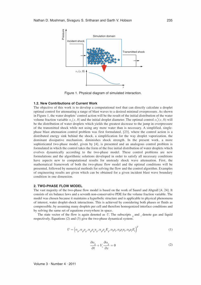
1.2. New Contributions of Current WorkThe objective of this work is to develop a computational tool that can directly calculate a dropletoptimal control for attenuating a range of blast waves to a desired minimal overpressure. As shownin Figure 1, the water droplets’ control action will be the result of the initial distribution of the watervolume fraction variable αl(x , 0) and the initial droplet diameter. The optimal control αl

*(x , 0) willbe the distribution of water droplets which yields the greatest decrease to the jump in overpressureof the transmitted shock while not using any more water than is necessary. A simplified, single-phase blast attenuation control problem was first formulated, [23], where the control action is adistributed energy sink behind the shock, a simplification for the way droplet vaporization, thedominant dissipative mechanism, diminishes shock strength. In the present work, a moresophisticated two-phase model, given by [4], is presented and an analogous control problem isformulated in which the control takes the form of the free initial distribution of water droplets whichevolves dynamically according to the two-phase model. These control problems are newformulations and the algorithmic solutions developed in order to satisfy all necessary conditionshave aspects new to computational results for unsteady shock wave attenuation. First, themathematical framework of both the two-phase flow model and the optimal conditions will bepresented, followed by numerical methods for solving the flow and the control algorithm. Examplesof engineering results are given which can be obtained for a given incident blast wave boundarycondition in one dimension.

2. TWO-PHASE FLOW MODELThe vast majority of the two-phase flow model is based on the work of Saurel and Abgrall [4, 24]. Itconsists of six balance laws and a seventh non-conservative PDE for the volume fraction variable. Themodel was chosen because it maintains a hyperbolic structure and is applicable to physical phenomenaof interest, water droplet-shock interactions. This is achieved by considering both phases or fluids ascompressible, by assuming many droplets per cell and therefore homogenized interface conditions andby solving the same set of equations everywhere in space.

The state vector of the flow is again denoted as U. The subscripts g and l denote gas and liquidrespectively. Equations (2) and (3) give the two-phase dynamical system.

(1)

(2)∂

∂+

∂

∂=

α αgi

g

tV

x0

U u E u Eg g g g g g g g g l l l l l l l l= (α α ρ α ρ α ρ α ρ α ρ α ρ, , , , , , ))T

Nathan D. Moshman, Sivaguru S. Sritharan and Garth V. Hobson 235


Simulation domain

Transmitted shock

Incident shock

Pre

ssur

e

αl (x, 0)

x

Figure 1. Physical diagram of simulated interaction.

The gas phase obeys the ideal gas equation of state while the stiffened gas equation of state is usedfor the liquid.

(4)

(5)

γ = 1.4 is the gas constant of air, γl = 4.4 is the analogous constant for water and πl = 6 ·108 Pa isthe stiffening constant that makes large changes in liquid pressure produce almost no changes indensity. Equations (6) and (7) are closure relations for the internal energy ρe to the total energy ρE, perunit volume, for each phase.

(6)

(7)

The volume fraction will propagate at a mean inter-facial velocity which is a center-of-mass estimategiven in eqn (8).

(8)

Ei and Pi are volume averages of total energy and pressure respectively at the interface shownin eqn (9).

(9)

The sum of the volume fractions of each phase will always equal 1 everywhere in the one-dimensional simulation domain. When either volume fraction tends toward zero, the 1D Euler systemis recovered.

(10)

Let U be the state vector in primitive form in eqn (11). The two-phase system can then be writtenin non-conservative form in eqns (12–13).

(11)U u P u Pg g g g l l l

T= ( )α ρ ρ, , , , , ,

α αg l+ = 1

E E E

P P Pi g g l l

i g g l l

= +

= +

α α

α α

Vu u

ig g g l l l

g g l l

=+

+

α ρ α ρ

α ρ α ρ

ρ ρ ρl l l l l lE e u= +1

22

ρ ρ ρg g g g g gE e u= +1

22

ρπ γ

γl ll l l

l

eP

=+

−1

ργg g

geP

=−1

(3)∂∂

t

u

E

u

E

g g

g g g

g g g

l l

l l l

l l l

α ρ

α ρ

α ρ

α ρ

α ρ

α ρ

+∂

∂

+

+( )x

u

u P

u E P

g g g

g g g g g

g g g g g g

l

α ρ

α ρ α

α ρ α

α ρ

2

ll l

l l l l l

l l l l l l

u

u P

u E P

α ρ α

α ρ α

2 +

+( )

=

−

−

0

0

P

PV

P

PV

i

i i

i

i i

∂

∂+

αg

xS U( )



(12)

The source term H(U) which multiplies in eqn (3) has been coupled into the Jacobian matrixin eqn (13) and the two-phase quasi-linear system now has simply the form shown in eqn (12).

With this fortunate manipulation, the seven eigenvalues can be found by diagonalizing A(U ). Thecharacteristic speeds are (Vi, ug, ug − cg, ug + cg, ul, ul − cl, ul + cl), where cg and cl are the localspeeds of sound in the gas and liquid phases respectively. The velocity of the phase interface is theseventh characteristic wave speed of the system. All are distinct except locally where they aredegenerately zero.

The source vector S(U) is broken up into three separate interactions as defined in eqn (14).

The source vector for mass and heat exchange between the phases is denoted as MH(U). The sourceterms for velocity and pressure equilibration are VR(U) and PR(U) respectively. As is pointed out in[4], an interface separating two phases must reach the same pressure through microscopic interactions.Indeed, without enforcing this condition, notions of thermodynamic properties such as temperaturecannot be determined and numerical oscillations due to pressure differences will grow withoutsignificant artificial dissipation [25].

The equilibrium condition Pg = Pl is chosen thereby neglecting the effect of surface tension. Themicroscopic pressure equilibration causes a volume and internal energy variation of each phase.Isolating the ODE = PR(U) in eqn (14) yields conditions better suited to computation.

(15)

(16)∂

∂= − −

α ρµg g g

i g l

E

tP P P( )

∂

∂= −

αµg

g ltP P( )

∂∂Ut

(14)S U MH U VR U PR U

mmV

m L E Qi

hv i i( ) ( ) ( ) ( ) ( )= + + = + +

0

−−−

− + −

mmV

m L E Qi

hv i i( )

+

0

0

F

Fd

dd i

d

d i

V

F

F V

0

−

−

+

−

−

µ

µ

( )

(

P P

P

g l

i

0

0

PP P

P P P

g l

i g l

−

−

)

( )

0

0

µ

∂

∂

αg

x

(13) AU

V

V u u

u

i

i g g g

P Pg

g

g

g i

g g

( )

( )

=

−

−

0 0 0 0 0 0

0 0 0 0

0 1

ρ

α

α ρ

ρ

//

( )

( )

ρ

ρρ

α

ρ

α

g

ci g g g g

i l

g gi

g

l

l

V u c u

V u

0 0 0

0 0 0 0

0 0 0

22−

− uu

u

V u c

l l

P Pl l

ci l l

l i

l l

l li

l

ρ

ρ

ρ

α ρ

ρ

α

0

0 0 0 0 1

0 0 0 02

−

−

/

( ) ll lu2

∂

∂+

∂

∂=

U

tA U

U

xS Ui

ijj

i( ) ( )



(17)

Inserting eqn (15) into eqns (16–17) reduces the ODE system to eqns (18–19).

(18)

(19)

In a closed system, this is just the first law of thermodynamics for an isentropic transformation. Timeintegration of both sides yields conditions given in eqn (20) and (21) whose solution is achieved via aNewton method which iteratively solves for αg

PR.

(20)

(21)

The superscript PR denotes the solution to the ODE for pressure relaxation while 0 denotes thestarting value which comes from the solution to the balance PDE at the current time step. The drag forceFd exerted by the gas onto a spherical water droplet, which is responsible for the VR(U ) source term,is given by the empirical drag law in eqn (22) where Dp is the diameter of the water droplet.

(22)

The droplets’ diameter is a dynamic variable distributed in space with the assumption of locallymono-dispersed droplets. Cd is a constant drag coefficient.

The exchange of mass and heat between the phases will be mainly due to vaporization of liquidwater droplets by the surrounding gas. The rate of gaseous mass production in the form of water vaporfrom the liquid phase, m , is defined in eqn (23).

(23)

The rate of change of the volume fraction of water within a fixed volume of space ∆x3 is related tothe diameter rate of change via eqn (24).

(24)

Sp denotes the total surface area of droplets per a fixed volume defined in eqn (25).

(25)SD

Npp

p=

4

2

2

π

αlp pS

x

D

t=

∆

∂

∂3

m PH Ov g l= ( )ρ α2

F C D u ud d g p l g l= −ρ α2 2( )

α ρ α ρ αα

α

l l lPR

l l l i gE E P dg

gPR

( ) −( ) = − ⋅∫0

0

α ρ α ρ αα

α

g g g

PR

g g g i gE E P dg

gPR

( ) −( ) = ⋅∫0

0

∂

∂= −

∂

∂

α ρ αg l li

gE

tP

t

∂

∂=

∂

∂

α ρ αg g gi

gE

tP

t

∂

∂= − −

α ρµg g g

i g l

E

tP P P( )



Np is the number of droplets per the same fixed volume as is uniquely determined by the volumefraction of water αl for mono-dispersed droplets.

(26)

The evolution of droplet size needed in eqn (26) is determined by the rate of vaporization. In thiswork, the Empirical-Beta vaporization law is implemented with constant values coming from [12].

(27)

(28)

As will be demonstrated in the Results section, the range of pressure magnitude for the flows ofinterest to the IOP attenuation problem are from 1–10 atm. According to steam tables [26], the watervapor density will vary by an order of magnitude over this pressure range. Consequently, water dropletvaporization will be much more effective to high pressure shocks. Equation (29) is the least-squaresquadratic fit to the steam table data for water vapor density as a function of the surrounding gas pressure.

(29)

The last term in the MH(U) vector, Qi, is the rate of heat exchange between phases at the interface,given in eqn (30) where h is the heat transfer coefficient.

(30)

For water droplets of diameter Dp, where Nu is the Nusselts Number and λ = 0.6 W/mK,

is the thermal conductivity of water.

2.1. Well-PosednessThe eigenvalues of A above are (Vi , ug , ug –cg , ug + cg , ul , ul –cl , ul + cl ). From the definition forinterface velocity and sound speeds it can be seen that all these eigenvalues are real and distinct if a fewconditions hold. If there are regions in our domain where a single phase is completely absent, then theinterface velocity will be degenerate to the velocity of the phase 100% present. Therefore, our calculation restricts the volume fraction of either phase to remain above a certain small threshold. As with the single-phase Euler system in one dimension, well-posedness can be shown by the existence of a real, positive-definite symmetrizer. It was shown by [27] that a necessary condition on the positive-definiteness of thesymmetrizer depends on the positiveness of a certain constitutive variable that should always physically bepositive such as density, temperature etc. The two-phase system has the same requirement. The Jacobianmatrix in eqn (13) is symmetrizeable if, in addition to the restriction that density and temperature remainpositive, the volume fraction of each phase remain non-zero. Since our model dictates that the sameequations be solved in each cell, no further care is needed to maintain well-posedness.

3. METHOD OF SOLUTION FOR TWO-PHASE GAS-LIQUID COUPLINGThe two-phase balance equations, point-wise relations, interface quantities and source terms defined inthe previous section are the basis for the overarching numeric method used to couple the two-phasesystem. While defining the mathematical model is essential to describing the optimal control system,the details of the numeric method for solving the flow are summarized for brevity and the reader isreferred to [4] for greater detail.

h NuDp

=λ

Q hS T Ti p g l= −( )

ρH Ov g g gP atm P P2

0024344 5368 077242( / ) . . .≈ − ⋅ + ⋅ − 66 3kg m/

β µ( ) ( . ( ) ) /.T T K m sg g= + ⋅ −−+7600 1 7 4 10 3007 2 7548 2

∂

∂= −

D

tTp

g

2

β( )

N x

Dp l

p

= ⋅∆

α

π

3

3

4

3 2



The sequence of numeric operations which progresses the solution from the nth to the (n + 1)th

time-step are given in eqn (31).

(31)

The operator Lh represents solving the discretization of the hyperbolic system shown in eqn (32).

(32)

The operator Ls represents solving the discretization of the three separate source terms systemshown in eqns (33–34).

(33)

(34)

A conservative Godunov method [28], second-order accurate in space, is used to solve the system ineqn (32). Details on that method are described in [29]. In order to maintain second order accuracy, thesolution involving the source term operators must therefore be performed for a half time-step as isshown in eqn (31), [30].

Details on the method of evolution of the droplets’ sizes and other properties related to vaporizationare provided since they were developed specifically for the current work. The present calculationassumes that droplets are mono-dispersed and spherical. Their initial size is denoted Dp

0(xi, 0). Whensurrounded by hot gas, the droplets will start to vaporize and their diameter will evolve according toeqn (35), a discrete integration of eqn (27).

(35)

Once the new size of the droplets are known, the added amount of gas volume fraction is known.

(36)

The critical quantity for sinking energy from the gas via vaporization is m which is given in discreteform below based on eqn (37).

(37)

The density of water is calculated from eqn (29).With the additional mass of water vapor in the gas phase, the gas density will increase according to

eqn (38) while the density of liquid water does not change.

(38)

The last source term operator in eqn (34), LMH, can now be integrated since the terms definingMH(U) in eqn (14) are now known at the current time-step.

4. DERIVATION OF NECESSARY CONDITIONS OF OPTIMAL SYSTEMOptimal control of fluid dynamics has undergone rapid developments during the past two decades[31–33]. Optimal control theory of hyperbolic systems of conservation laws for applications of gasdynamics with shock waves is addressed in [34, 35]. This section gives a brief derivation of all first order

ρ α ρ αgn

gn

gn

gnm+ += +1 1( )/&

&m x t P x t atm x tin

H Ov g in

g in( , ) ( ( , ) / )( ( ,+ +=1

21ρ α ++ −1) ( , ))αg i

nx t

α α πgn

gn p

npnD D

++

= + −

11

4

3 2 2

3 3

NNpn

D x t D x t t T x tp in

p in

g in2 1 2( , ) ( , ) ( ( , ))+ = − ∆ ⋅ β

L L L Ls MH VR PR≡ ⋅ ⋅

L Ut

S Us : ( )∂∂

=

L Ut

F U H Uxh xg: ( ) ( )

∂∂

+ =∂

∂

α

U L L L Uns

th

ts

t n+ =1 2 2 2/ / /∆ ∆ ∆



necessary conditions of optimality. Let a nonlinear partial differential operator N, which operates on astate vector U and control vector z take the form of eqn (39).

(39)

After the dynamical system is known, a cost, or objective, functional must be intelligently defined.In the most general framework there can be a cost associated with the initial data I, a cost involving thefinal data K and a running cost L that accumulates over the time interval of the control problem [0, T ].So far, initial and final data can still be free or fixed, no restriction has been made. The cost functionalsdescribe the objective associated with how these parameters are distributed. Let J be the total costfunctional.

(40)

To incorporate the constraint in the minimization, N is multiplied by a generic continuous vector V (x, t) and added to J. The problem then becomes minimizing the augmented cost functional J .

(41)

It is standard to refer to Vi(x, t) as the costate or adjoint vector. It is a m-dimensional vector sincethere is an adjoint state for every state variable. The notation (·, ·) signifies a spatial integral.

Let (z*, U *, V*, T*) be the optimal control, state vector, adjoint vector and final time respectively.Let a perturbed control function δz be added to the optimal control solution so that:

(42)

where ε > 0 is a small constant. The perturbed optimal control introduces a perturbation to theoptimal state and adjoint state:

(43)

(44)

Another way to see δU which will be useful shortly is:

(45)

It has been pointed out in the literature [36–38] that if the state variables have shocks, a perturbationis not small in the neighborhood of the shock and does not have the vanishing properties as ε → 0. Aslight increase in the amplitude behind the shock perturbs the shock speed and therefore also thelocation of the shock front. This causes small perturbations to induce variations on the order of the jumpacross the shock. The presented method of solution avoids this issue, as will be demonstrated later.Since only decreasing the amplitude of a shock wave is desired it is apparent that any realistic controlaction will only slow the shock wave down. The target state Q(x) and final time penalty will beconstructed in such a way that all variations of the solution will occur upstream of the shock front only.Matching the simulated pressure profile under control action with the target final state near the shockfront will occur by allowing the final time to be free. Henceforth, it can be assumed that all variationsare taken in smooth regions of the flow and that the solution procedure will not depend on an additionalshock location variable and corresponding adjoint state, nor is a different type of variation required.

The first order necessary optimal condition that must be satisfied by a perturbed control, state,adjoint state and final time (δz, δU, δV, δt ) is:

δ δU dd

U z z= + =εε ε( )* | 0

V V V= +* εδ

U U U= +* εδ

z z z= +* εδ

%J I U K U T L U z V N U z dt= + + +( (., )) ( (., )) ( , ) ( , ( , ))00

TT

∫

J I U K U T L U z dtT

= + + ∫( (., )) ( (., )) ( , )00

N U zUt

A UU

xS U zi

ijj

ki i( , ) ( ) ( )=

∂

∂+

∂

∂− − = 0



(46)

Equations (47–50) are what is obtained after expanding all of the terms and grouping the ones withlike variations. xR and xL denote the right and left points of the spatial boundary in a single dimension.

(48)

(49)

Recall that the final time is free to vary. Therefore, a necessary condition for the final time must beconstructed. This is known as the Transversality condition. The variation of the state at the final time

will have a first order term expanded in space . Therefore, there is a

change to the final time boundary condition.

(50)

The pseudo-Hamiltonian is defined in general in eqn (51).

(51)

Using this definition, the Transversality Condition takes it’s familiar form in eqn (52).

(52)

5. TWO-PHASE CONTROL PROBLEM FORMULATION AND SOLUTIONThe solution procedure will iteratively reach a control, state, adjoint and final time that satisfy all firstorder necessary conditions. An adjoint PDE must be solved backward in time to fix an initial conditionon a free state variable. The cost functional J, given in continuous form in eqn (53) and shown indiscrete form in eqn (56), will be minimized while all constraints of the two-phase model are obeyed.

(53)J a x dx b P x T Q x dxl gs

= ( ) + −( )Ω

+Ω

∫ ∫20

2

2 2α ( , ) ( , ) ( )

δt H dKdtt T, *|

=+

= 0

H L V Ut

= +∂∂

,

δ δ δU x T U x Tt

t KU

V U( , )( , )

, *+∂

∂∂∂

+

= ,, ,* *∂∂

+

+∂∂

∂∂

+

KU

V t Ut

KU

Vδ

δ δ δU x T U U x Tt

t( , )( , )

= +∂

∂

∂∂

+

=KU

V x T U x T*( , ), ( , )δ 0

∂∂

−

=IU

V x U x*( , ), ( , )0 0 0δ

(47)

∂∂

−

+

−∂

∂+

∂

∂

∫Lz

V z x t

V

t

A

U

T

j ij

k

*

*

, ( , )δ0

∂∂

∂−

∂

∂

−

∂

∂−

∂

∂

Ux

A

xV A

Vx

SU

k iji ij

i i**

jji

jj

ij i j

V LU

U

xA V U

*

*

,

,

+∂

∂

+

−∂

∂

δ

δ(( )

=

=+ + =

=

x x

x xL V N U z tR

L t T

( ( , ( , )))* * * δ 0

dd

J z zε

ε ε%( )* + ==δ | 0 0



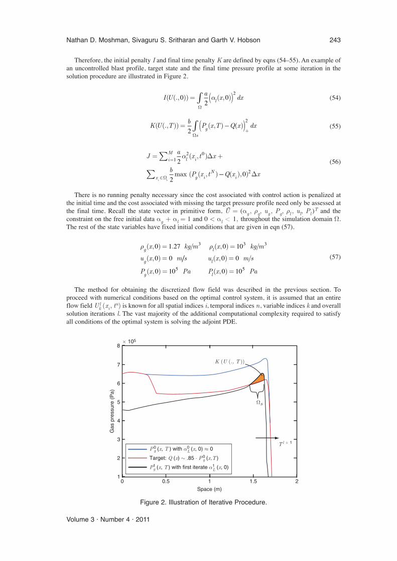
Therefore, the initial penalty I and final time penalty K are defined by eqns (54–55). An example ofan uncontrolled blast profile, target state and the final time pressure profile at some iteration in thesolution procedure are illustrated in Figure 2.

(54)

(55)

(56)

There is no running penalty necessary since the cost associated with control action is penalized atthe initial time and the cost associated with missing the target pressure profile need only be assessed atthe final time. Recall the state vector in primitive form, U = (αg , ρg, ug , Pg, ρl , ul, Pl )

T and theconstraint on the free initial data αg + αl = 1 and 0 < αl < 1, throughout the simulation domain Ω.The rest of the state variables have fixed initial conditions that are given in eqn (57).

(57)

The method for obtaining the discretized flow field was described in the previous section. Toproceed with numerical conditions based on the optimal control system, it is assumed that an entireflow field Ul

k (xi, tn) is known for all spatial indices i, temporal indices n, variable indices k and overallsolution iterations l. The vast majority of the additional computational complexity required to satisfyall conditions of the optimal system is solving the adjoint PDE.

ρ ρg l

g

x kg m x kg m

u x m

( , ) . / ( , ) /

( , )

0 1 27 0 10

0 0

3 3 3= =

= // ( , ) /

( , ) ( , )

s u x m s

P x Pa P x Pal

g l

0 0

0 10 0 105 5

=

= =

J a x t x

b P x t

l iiM

x g iN

i s

= ∆ +=

∈Ω

∑

∑2

2

2 01

α ( , )

max ( ( , )−− ∆Q x xi( ), )0 2

K U T b P x T Q x dxgs

( (., )) ( , ) ( )= −( )+

Ω∫2

2

I U a x dxl( (., )) ( , )02

02

= ( )Ω∫ α



7

T l + 1

K (U (., T ))

8

6

5

4

3

Space (m)

Gas

pre

ssur

e (P

a)

2

0.51

0 1 1.5 2

Ωs

P 0 g (x, T ) with α0 L (x, 0) ≈ 0

Target: Q (x) ∼ .85 ⋅ P 0 g (x,T )

P1g (x, T ) with first iterate α1 L (x, 0)

× 105

Figure 2. Illustration of Iterative Procedure.

It is convenient to define the target state in terms of the pressure. Since the Jacobian has already beenprovided in the primitive basis in [4] the adjoint PDE is simpler to derive in that same basis. The non-trivial elements of the matrices are given in [39]. The necessary condition on the adjoint vector at thefinal time is given for all xi ∈ Ωs. As shown in Figure 2, Ωs is defined as the region in space where aniterate of the final time pressure is greater than the target state.

(58)

Starting with the final time boundary condition in eqn (58), the adjoint PDE can be solved backwardin time to arrive at a value for Vl

1 (xi, 0). From the necessary condition given in eqn (48), the volumefraction of liquid at each point in space will be iterated, within the constraints, via a fixed-point Newtonmethod shown in eqn (59).

(59)

A survey of the literature on adjoint-based methods for optimal control [40–43] gave insight on howto construct a solution algorithm. However, there were no methods specifically for distributed controlwith free initial and final data and final time for unsteady shock attenuation.

To solve for the optimal final time, the Transversality Condition for the two-phase system, given ineqn (52), is defined as a continuous function f(T) with the final time as the independent variable. Thenf (T*) = 0 at the optimal final time T*. The optimal final time, T*, can be solved iteratively with theNewton method from using the discretization of f in eqn (60).

(60)

The definition of and its discretization are also given in [39]. The overall algorithm which is used

to satisfy all of the above necessary optimal conditions is shown in block-diagram form in Figure 3.The continuous form of the adjoint PDE system is shown as the pairing with δUj in eqn (47). The

system is linear in the adjoint variables. The time derivative of the entire adjoint vector for all space ata discrete time tn is shown in column-upon-column form in eqn (61). Let m be the number of spatialgrid points and k be the number of adjoint variables. Then the adjoint vector V at a discrete moment intime will be of size km by 1 and the matrices in eqn (47) will be of size km by km. A single componentof the adjoint vector, eg. V1(x, t), will be size m by 1 at each time step.

(61)

∂

∂↔

∂∂

( )

( )

Vt t

V x t

V x t

kl

n

mn

1 1

1

,

,

M

( )

( )

V x t

V x t

n

mn

2 1

2

,

,

M

( )

(

M

M

V x t

V x t

kn

k mn

1,

, ))

dfdt

f T P x t Q xP x t P x t

lg i

Ni

g iN

g iN

( ) = ( )− ( )( ) ( )− ( −

,, , 1))

=∑∆

∆t

xim

1

α αα

gl

i gl

igl

il

ix t x t

a x t V x t+ ( ) = ( )−

− ( )( )−1 0 0

011

, ,, , 00

1 11( )

−= −+ +

a ll

llα α

V x T b P x T Q x kkl

il i

li( , )

max (( ( , ) ( )), )=

⋅ −

=0

0

4kk ≠ 4



All of the matrices in eqn (47) have a diagonal-block structure. The Jacobian matrix for all of spaceat tn is shown in eqn (62).

The adjoint PDE is given in discrete form with an explicit integration in eqns (63–64).

(63)

(64)R U A DU Ax

AU

Ux

SU

( ) = ⋅ +∂∂

−∂∂

⋅∂∂

+∂∂

101

∆−( )+ =−

tI V V R U Vk

nkn n

in( )

(62)

A U

A x t

A x t

kn

n

mn

ν( )

( , )

( , )

↔

11 1

11

O

L O

A x t

A x t

kn

k mn

1 1

1

( , )

( , )

M O M

O

A x t

A x t

kn

k mn

1 1

1

( , )

( , )

L O

A x t

A

kkn

kk

( , )

(

1

xx tmn, )



Calculate cost

Iterate T l+1 according tonewton method

Calculate intial data iterateαl

l+1 (x, 0) from adjoint Vll+1 (x, 0)

Solve two phase flow withnew initial condition αl

l+1 (x, 0)

Using final time conditionsolve adjoint PDEbackward in time

Converge to optimal(U ∗, V ∗, T ∗)

Set target state

Solve two phase flowwith no control

Gradually decreaseamplitude oftarget state

Output

Figure 3. Block diagram of solution procedure for two-phase control calculation.

The matrix D is made up of discrete spatial derivative block matrices, central differencing in the domaininterior, upwind differencing at the outlet and downwind at the inlet. A single block is shown in eqn (65).

For adjoint calculations of a scalar PDE with a discontinuity, it has been shown [44, 45] that arelaxed system with second order dissipation will recover the non-linear PDE in the limit of vanishingviscosity. A small numerical viscosity can stabilize the adjoint solution. These ideas have been extendedto fluid dynamics systems in [45] and are implemented in the current work, in a manner whichmaintains consistency for the two-phase numerical adjoint solutions.

6. RESULTSData on the shuttle grain and chamber pressure from [46] was input to Cequel [47] a code for steadystate rocket property calculations. The output gives the temperature and gas velocity at the nozzle exitplane for a given pressure ratio. Initially, ambient conditions inside the domain are present. The ignitionsequence was simulated in 2D using the ESI-Fastran commercial software, [48]. The spatialdiscretization scheme used was Van Leer’s flux vector splitting and was extended to second orderaccuracy by a Barth limiter. The Barth limiter enforces monotonicity and, therefore, is appropriate forsolutions with strong discontinuities. Time integration was fully implicit with a tolerance of 10−4 in theresiduals over a maximum of 20 sub-iterations.

Constant mass-flow boundary conditions equivalent to the steady state exit plane of the rocketnozzle on the shuttle were used in the bottom center of the domain on the right face of the step as shownin Figure 4.a. Mach number is depicted in three snapshots in Figure 4.a, 4.c and 4.e and pressure inFigure 4.b, 4.d, and 4.f. The last frame is roughly 10 ms after ignition. The bottom left edge of thedomain represents the rocket body while the bottom right edge is the centerline of the normal to thenozzle exit plane and a symmetry boundary. All other edges are non-reflecting boundaries.

Flow conditions over time were recorded at two locations marked in Figure 4.a. Point 1 is near therocket body 2.5 meters above the nozzle and Point 2 is 1.5 meters along the symmetry boundary andthe plane normal to the nozzle exit. The conditions at the recorded locations are used as the boundaryconditions in both the single- and two-phase control calculations.

Figure 5.a shows the flow conditions over time at Monitor Points 1 near the rocket body and Figure5.b shows the flow conditions over time for Monitor Point 2 directly downstream of the nozzle.

It is worth mentioning that the two-dimensional flow cannot be truly replicated by an inlet boundarycondition to a single-dimensional calculation. Neglecting motion in the transverse direction whiletaking (ρ, u , P) explicitly means that the resulting driver gas has a lower temperature. This is notdiscouraging since intuition would suggest that hotter gas has more potential to vaporize water dropletsand hence, by the nature of the control action, there is more potential for effectiveness. The goal is tobe able to handle a range of blast waves that will plausibly be seen in an IOP environment.

The results for the two-phase control problem were obtained with the algorithm shown in Figure 3.In each case, the spatial grid size was 1 cm and the time-step was 1 µs. Figure 6.a shows the optimalinitial condition for the free water volume fraction variable. The inlet condition is given by the datafrom Monitor Point 1 pictured in Figure 4.a and graphed over time in Figure 5.a. The curves give theoptimal water volume fraction distributions for four target states with successively decreasing jumps inpressure at the shock front. The legend tells what percentage of the absolute overpressure of theuncontrolled blast wave was used to define the target state.

Figures 7.a and 7.b are analogous to Figure 6.a and 6.b except that now the driving inlet boundarycondition is from Monitor Point 2; which is pictured in Figure 4.a and graphed over time in Figure 5.b.Monitor Point 1 data gives a shock with a little less than a 2:1 jump in pressure at the shock front, anda driving gas temperature of less than 500 K. Monitor Point 2 data gives a shock with about an 8:1 jumpin pressure at the shock and a driving gas temperature of more than 1000 K. Several differences in the

(65)Dxmxm =

∆

−−

−−

1

2

2 2

1 0 1

1 0 1

2 2

O O O





Mach3.414

Mach3.414

3

(a) (b)

(c) (d)

(e) (f)

2.5

2

1

2

1.5

1

0.5

3.358E-021

3.358E-021

3

2.5

2

1.5

1

0.5

6E+005

5E+005

4E+005

3E+005

2E+005

1E+005

2.635E+004

p − N/m^26.845E+005

6E+005

5E+005

4E+005

3E+005

2E+005

1E+005

6E+005

5E+005

4E+005

6E+005

2E+005

1E+005

p − N/m^26.845E+005

2.635E+004

Mach3.414

3.358E-021

3

2.5

2

1.5

1

0.5

p − N/m^26.845E+005

2.635E+004

Figure 4. Simulated Shuttle IOP: Mach Number at (1.2 ms, 4 ms, 10 ms) after ignition(a, c, e); Pressure at (1.2 ms, 4 ms, 10 ms) after ignition (b, d, f).

0.00100

5

1000

−1000

0

0.002 0.003 0.004 0.005 0.006 0.007 0.008 0.009 0.01

0.0010 0.002

Den

sitiy

(kg

/m3 )

Vel

ocity

(m

/s)

Pre

ssur

e (P

a)

0.003 0.004 0.005 0.006 0.007 0.008 0.009 0.01

3× 105

1

2

0.0010 0.002 0.003 0.004 0.005 0.006 0.007 0.008 0.009 0.01

0.00100

5

4000

0

2000

0.002 0.003 0.004 0.005 0.006 0.007 0.008 0.009 0.01

0.0010 0.002

Den

sitiy

(kg

/m3 )

Vel

ocity

(m

/s)

Pre

ssur

e (P

a)

0.003 0.004 0.005 0.006 0.007 0.008 0.009 0.01

10× 105

0

5

0.0010 0.002 0.003 0.004 0.005 0.006 0.007 0.008 0.009 0.01

(a) (b)

Time (s) Time (s)

Figure 5. Flow conditions over time for Monitor Point 1 (a) and Monitor Point 2 (b).

solution are worth noting as they give insight into how differently the water droplets affect blast wavesover the range of overpressure that may be encountered in an IOP environment.

The largest fractional decrease in overpressure achievable in 2 ms with with the MP1 inlet conditionis 87.5% of the uncontrolled wave, (OP0) while the largest fractional decrease in overpressure achievable(in the same time interval) with with the inlet condition of MP2 is 76% of the uncontrolled wave. Noticethat the MP2 shock travels nearly twice as far as the MP1 shock. The shape and maximum height ofthe optimal water distributions for these two cases are nearly the same. This shows that the water dropletsare able to affect a greater decrease in shock strength when the shock is driven by hotter gas since hottergas will vaporize water more quickly and cause a larger decrease in the pressure of the gas pushing theshock. This is illustrated in Figure 6.b and 7.b. Notice that in Figure 6.b, the most attenuated shock profileis flat while this is not true of the most attenuated profile in Figure 7.b. The difference comes from the gastemperature. The lower temperature gas from the MP1 data has entirely cooled to about 300 K at the endof the simulation which leaving no more potential for droplet vaporization. In contrast, the hottertemperature gas from the MP2 data has not yet entirely cooled to 300 K, meaning that further dropletvaporization is possible and that the pressure profiles have yet to flatten out.



95% OP0

95% OP0

OP0

× 105(b)(a)

92.5% OP0

92.5% OP090% OP0

90% OP087.5% OP0

87.5% OP0

2

1.9

1.8

1.7

1.6

1.5

1.4

Gas

pre

ssur

e (P

a)

1.3

1.2

1.1

1

1

0.9

0.8

0.7

0.6

0.5

0.4

Gas

pre

ssur

e (P

a)

Space (m)

0.3

0.2

0.1

00 0.1 0.2 0.3 0.4 0.5 0.6 0.7 0.8 0.9 1

Space (m)

0 0.1 0.2 0.3 0.4 0.5 0.6 0.7 0.8 0.9 1

Figure 6. (a) Unconstrained optimal water volume fraction distributions at initial moment intime αl* (x, 0) for MP1 inlet condition (b) Optimal final time pressure profiles P* (x, T *)

resulting from initial data in Figure a.

00 1.20.2 1.40.4

Space (m)

Vol

ume

frac

tion

1.60.6 1.80.8 1 2 01

2

3

4

5

6

7

8

1.20.2 1.40.4 1.60.6 1.80.8 1 2

Space (m)

0.1

0.2

0.3

0.4

0.5

0.6

0.7

0.8

0.9

1(b)(a)

Gas

pre

ssur

e (P

a)

× 105

85% OP082% OP079% OP076% OP0

85% OP0

OP0

82% OP079% OP076% OP0

Figure 7. (a) Unconstrained optimal water volume fraction distributions at initial moment intime αl* (x, 0) for MP2 inlet condition (b) Optimal final time pressure profiles P* (x, T *)

resulting from initial data in Figure a.

The convergence of the algorithm is shown in Figure 8.a. Every 25 iterations, the target state’samplitude is ramped down so that optimal solutions that yield ever increasing attenuation levels can bedetermined in a single execution of code. The history of the final time variable over the iterativesolution procedure is shown in Figure 8.b. As the final time changed, the time-step size changed slightlyfrom 1 µs so that the nearest integer number of time-steps yielded the final time iterate.

If the target amplitude is set too low, first-order variation conditions fail to maintain convergence ofthe overall algorithm. The argument that the solution is indeed a minimum can be readily illustrated inFigure 8.a. The final time penalty is weighted to a much larger magnitude than the initial penaltythereby ensuring that the solution definitely is one which attenuates the shock wave. At the same timethe control action is ever-increasing at a decreasing rate. Therefore, if less control is used, J willincrease because K will increase. Similarly if more control is used J will still increase because I willincrease and K cannot decrease any further.

Another case was run with an upper bound on the volume fraction of water at 70%. The calculatedoptimal water distributions are shown in Figure 9.a with the resulting pressure profiles shown in Figure 9.b.



00

0.12.02

2.04

2.06

2.08

2.1

2.12

2.14

0.2

0.3

0.4

0.5

10 20 30 40 50

Nor

mal

ized

cos

t

60 70 80 90 101 20Iteration Iteration

30 40

Fin

al ti

me

(s)

50 60 70 80 90 100100

0.6

0.7

0.8

0.9

1(b)(a)

Initial costFinal costTotal cost

× 10−3

Figure 8. (a) Cost functional J in red and initial penalty I over iterations of solution procedure(b) Final time, in seconds, vs iteration number for the unconstrained case. The regions of

greatest slope are after iterations where the target state has been changed. The slope tendingtoward zero means that the solution for the optimal final time is converging.

0.9

1

0.8

0.7

0.6

0.5

0.4

0.3

0.2

0.1

0.20 0.4 0.6 0.8 1Space (m)

Vol

ume

frac

tion

1.2 1.4 1.6 1.8 20 0.20 0.4 0.6 0.8 1

Space (m)

Gas

pre

ssur

e (P

a)

1.2 1.4 1.6 1.8 2

2

1

3

4

5

6

7

8(a) (b) × 105

OP095% OP092.5% OP090% OP087.5% OP085% OP082.5% OP080% OP0

95% OP092.5% OP090% OP087.5% OP085% OP082.5% OP080% OP0

Figure 9. (a) Optimal initial water volume fraction distributions, αl(x, 0) ≤ .7 (b) The optimalpressure profiles at the final time resulting from the control initial data.

A final case was run, this time with an upper bound on the volume fraction of water at 50%. Thecalculated optimal water distributions are shown in Figure 10.a with the resulting pressure profilesshown in Figure 10.b.

A few more isolated results were obtained in the interest of categorizing the significance of modelparameters. Figure 11.a shows the effect of droplet size on overpressure attenuation. Each pressureprofile is plotted after two milliseconds of shock propagation from the left boundary toward the right.For a constant amount of water mass, more surface area of the droplets are exposed to the flow whenthe droplets are smaller. This is verified in eqn (66) for mono-dispersed droplets with diameter Dp.

This result agrees with empirical results, [15], that the more droplet surface area exposed, the greaterthe overpressure attenuation. Since surface area is maximized with infinitely small droplets, initialdroplet size isn’t an optimizeable parameter. Droplets with a diameter Dp = 25 µm were used in all ofthe preceding results since that size is small enough to have a significant effect over two meters, is areasonable size based on injector atomizer specifications and prevents the droplets from beingcompletely vaporized within the simulation time T*. Note that the result in Figure 11.a isolates theeffect of droplet size without considering droplet breakup which would presumably diminish thedifference in the results to some degree.

Water vapor density was shown to have a drastic effect on results for optimal water distributions.Water vapor density increases by an order of magnitude from ambient pressure to the 8 atm level behindthe shock front of the MP2 data. Therefore, if water vaporizes under high pressures, mass changesphase at a higher steam density and, consequently, the dissipative effect of vaporization is much moresignificant. The results in Figure 11.b show that more than twice as much water is needed to get 5%attenuation in pressure depending on the density of the water vapor produced.

(66)

SD

N

N x

D

pp

p

p l

p

=

⋅

=∆

42

4

3 2

2

3

π

α

π

⇒

3

1SDp

p

∼



0.9

1

0.8

0.7

0.6

0.5

0.4

0.3

0.2

0.1

0.20 0.4 0.6 0.8 1Space (m)

Vol

ume

frac

tion

1.2 1.4 1.6 1.8 20 0.20 0.4 0.6 0.8 1

Space (m)

Gas

pre

ssur

e (P

a)

1.2 1.4 1.6 1.8 2

2

1

3

4

5

6

7

8(a) (b) × 105

OP0

90% OP0

87.5% OP0

85% OP0

82.5% OP0

90% OP0

87.5% OP0

85% OP0

82.5% OP0

Figure 10. (a) Optimal initial water volume fraction distributions, αl(x, 0) ≤ .5 (b) Optimalfinal time pressure profiles resulting from initial data.

7. CONCLUSIONSA new iterative solution procedure was developed which can calculate optimal distributed controlsolutions for systems of quasi-linear hyperbolic partial differential equations with free initial and finaldata and final time. This procedure has been successfully applied to two-phase compressible gasdynamics in one dimension with the goal of diminishing overpressure at the shock front of a blast wavegenerated by an ignition overpressure. Examples of optimal attenuation to blast waves typicallyencountered in the launch environment of the Shuttle’s SRBs during an ignition are given. Optimalwater volume fractions are calculated for increasing levels of attenuation. Cases where the maximumvolume fraction of water is restricted to 50% and 70% are also presented.

The results give several key insights relevant to implementing water injection systems for blast waveattenuation. Smaller droplets will vaporize quicker since the total surface area exposed to the flow islarger resulting in cooler gas driving a shock with an attenuated jump at the shock front. This wouldsuggest that large regions of space completely filled with water are sub-optimal for blast attenuationsince connected streams or ligaments of water expose less surface area to the gas.

The degree of attenuation depends largely on the rate of mass changing phase from liquid water togaseous water vapor due to forced vaporization m, which is equal to the product of the water vapordensity and the rate of change of the volume occupied by the water droplets. In the high pressure andhigh temperature region behind the shock front, water vapor density is high and the rate of vaporizationis high as well which both contribute to a large value for m. As the control takes effect, the pressureand temperature of the gas both decrease meaning that the effects are being felt by the shock front at aslower rate. These results show that, in general, stronger shocks can be attenuated more rapidly thanweaker shocks via water droplet vaporization.

In a two meter domain using the MP2 data, 76% OP0 was the target with the lowest overpressurefor which the solution still converged. The case with the volume fraction of water restricted to amaximum of αl < 70% converged with the lowest target overpressure of 80% OP0. With the waterrestricted to below αl < 50% by volume, the most attenuation achievable with a two meter domain is82.5% OP0. In a one meter domain using the MP1 data, the lowest target state achievable was 87.5%OP0 .

ACKNOWLEDGMENTSN. D. Moshman would like to thank Professors Chris Brophy, Frank Giraldo and Wei Kang at theNaval Postgraduate School and Bruce Vu at NASA Kennedy Space Center. In addition, N. D.Moshman thanks the Naval Postgraduate School and the Army Research Office for funding thisresearch.



0.9

1(b)(a)

0.8

0.7

0.6

0.5

0.4

0.3

0.2

0.1

0.20 0.4 0.6 0.8 1Space (m)

Opt

imal

vol

ume

frac

tion

1.2 1.4 1.6 1.8 20

0.20 0.4 0.6 0.8 1Space (m)

Gas

pre

ssur

e (P

a)

1.2

25 µm50 µm100 µm250 µm

1.4 1.6 1.8 2

3

2

1

4

5

6

7

8

9× 105

1.5 kg/m3

2.0 kg/m3

2.5 kg/m3

3.0 kg/m3

3.5 kg/m3

4.0 kg/m3

Saturation

Figure 11. (a) effect of varying droplet size (b) effect of varying water vapor density.

REFERENCES[1] D. B. Kothe, and W. J. Rider, Comments on Modeling Inter-facial Flows with Volume-of-Fluid

Methods, Technical Report LA-UR-3384, Los Alamos National Laboratory, 1995.

[2] R. Caiden, R. P. Fedkiw, and C. Anderson, A Numerical Method for Two-Phase Flow Consistingof Separate Compressible and Incompressible Regions, Journal of Computational Physics, 166,2001, 1–27.

[3] C. A. Lowe, Two-phase Shock-Tube Problems and Numerical Methods of Solution, Journal ofComputational Physics, 204, 2005, 598–632.

[4] R. Saurel, and R. Abgrall, A Multiphase Godunov Method for Compressible Multifluid andMultiphase Flows, Journal of Computational Physics, 150, 1999, 425–467.

[5] S. Lai, and F. S. Laspesa, Ignition Overpressure Measured on STS Lift-Off and Correlation withSubscale Model Tests, JANNAF, 13th Plume Technology Meeting, 1982.

[6] E. J. Walsh, and P. M. Hart, Flight-Measured Lift-off Ignition Overpressure, A Correlation withSub-scale Model Tests, Martin Marietta Aerospace, AIAA Paper, 1981, 81–2458.

[7] D. Alvord, Ares 1-X Ignition Overpressure T+30 Day Analysis and Results, Jacobs ESTS Group,January 2010, Kennedy Space Center, FL, ESTSG-FY10-00793.

[8] W. G. Reinecke, and G. D. Waldman, A Study of Drop Breakup Behind Strong Shocks withApplications to Flight, AVCO Report, AD-871218, May 1970.

[9] J. Woo Jr., J. H. Jones, and S. H. Guest, A Study of Effects of Water Addition on Supersonic GasStreams, JANNAF, 13th Plume Technology Meeting, 1982.

[10] C. Crowe, M. Sommerfeld, and Y. Tsuji, Multiphase Flows with Droplets and Particles, CRCPress, New York, 1998.

[11] G. O. Thomas, On the Conditions Required for Explosion Mitigation by Water Sprays,Transactions of the Institution of Chemical Engineers, 78, Part B, September 2000, 339–354.

[12] D. Schwer, and K. Kailasanath, Blast Mitigation by Water Mist (2), Shock Wave Mitigation usingGlass Particles and Water Droplets, NRL Memorandum Report, January 21, 2003,6410–03–8658.

[13] R. Ananth, H. D. Ladouceur, H. D. Willauer, J. P. Farley, and F. W. Williams, Effect of Water Miston a Confined Blast, Suppression and Detection Research and Applications Technical WorkingConference (SUPDET), Orlando, FL., March 11–13, 2008.

[14] H. D. Willauer, R. Ananth, J. P. Farley, G. Back, M. Kennedy, J. O’Connor, and V. M. Gameiro,Blast Mitigation Using Water Mist: Test Series II, NRL Memorandum Report, March 12, 2009,6180–09–9182.

[15] G. Jourdan, L. Biamino, C. Mariani, C. Blanchot, E. Daniel, J. Massoni, L. Houas, R. Tosello, andD. Praguine, Attenuation of a Shock Wave Passing Through a Cloud of Water Droplets, ShockWaves, 20, No. 4, 2010, 285–296.

[16] H. Ikawa, and F. S. Laspesa, Space Shuttle SRM Ignition Overpressure Prediction Methodology,JANNAF, 13th Plume Technology Meeting, 1982.

[17] C. Kiris, W. Chan, D. Kwak, and J. A. Housman, Time-Accurate Computational Analysis of theFlame Trench, The Fifth International Conference on Computational Fluid Dynamics, Seoul,Korea, July 7–11, 2008.

[18] C. Kiris, J. A. Housman, and D. Kwak, Space-Time Convergence Analysis of a IgnitionOverpressure in the Flame Trench, CFD Review 2010, World Scientific.

[19] H. Ikawa, and F. S. Laspersa, Analytical Understanding of WTR Ignition/Duct OverpressureInduced by Space Shuttle Solid Rocket Motor Ignition Transient, AIAA/SAE/ASME 19th JointPropulsion Conference, Seattle, WA, June 27–29, 1983.

[20] J. Troyes, I. Dubois, V. Borie, and A. Boischot, Multi-phase Reactive Numerical Simulations of aModel Solid Rocket Motor Exhaust Jet, 42nd AIAA/ASME/SAI/ASEE Joint PropulsionConference and Exhibit, Sacramento, CA, July 9–12, 2006.

[21] F. Canabal III, Suppression of the Ignition Overpressure Generated by Launch Vehicles, Ph.D.Dissertation, Mechanical and Aerospace Engineering Department, University of Alabama,Huntsville, 2004.



[22] F. Canabal III, and A. Frendi, “Study of the Ignition Overpressure Suppression Technique byWater Addition,” Journal of Spacecraft and Rockets, 43, No. 4, 2006, 853–865.

[23] N. D. Moshman, G. V. Hobson and S. S. Sritharan, A Method for Optimally Controlling UnsteadyShock Strength in One Dimension, AIAA Journal, accepted for publication July 2012.

[24] R. Saurel, and R. Abgrall, A Simple Method for Compressible Multifluid Flows, SIAM Journal ofScientific Computing 21, No. 3, 2000, 1115–1145.

[25] R. Abgrall, How to Prevent Pressure Oscillations in Multicomponent Flow Calculations: A QuasiConservative Approach, Journal of Computational Physics, 125, 1996, 150–160.

[26] IAPWS Industrial Formulation 1997 for the Thermodynamic Properties of Water and Steam.(IAPWS-IF97)

[27] B. Texier, Lecture 2: Symmetrizable Systems, RMMC Summer School, Laramie, WY, June 2010.

[28] S. K. Godunov, A Finite difference Method for the Numerical Computation of DiscontinuousSolutions of the Equations of Fluid Dynamics, Matematicheskii Sbornik, 47, 1959, 257–393.

[29] B. Van Leer, Toward the Ultimate Conservative Difference Scheme (5) A Second-Order Sequelto Godunov’s Method, Journal of Computational Physics, 32, July 1979, 101–136.

[30] T. I. P. Shih, and W. J. Chyu, Approximate Factorization with Source Terms, AIAA JournalTechnical Notes, 29, No. 10, 1759–1760.

[31] Gad-el-Hak, M., Flow Control: Passive, Active and Reactive Flow Management, CambridgeUniversity Press, New York, 2000.

[32] Sritharan, S. S. editor. Optimal Control of Viscous Flow, SIAM Books, Philadelphia, PA, 1998.

[33] Gunzburger, M. D. Perspectives in Flow Control and Optimization, SIAM Books, Philadelphia,PA, 2003.

[34] A. Bressan, and A. Marson, A Maximum Principle for Optimally Controlled Systems ofConservations Laws, Rendiconti del Seminario Matematico della Universita di Padova, 94, 1995,79–94.

[35] Fursikov, A. V., Optimal Control of Distributed Systems: Theory and Applications. AmericanMathematical Society, Providence, Rhode Island, 2000.

[36] A. Bressan, and A. Marson, A Variational Calculus for Discontinuous Solutions to ConservationLaws, Communications on Partial Differential Equations, 20, 1995, 1491–1552.

[37] S. Ulbrich, A Sensitivity and Adjoint Calculus for Discontinuous Solutions of HyperbolicConservation Laws with Source Terms, SIAM Journal of Control and Optimization, 41, 2002,740–783.

[38] S. Ulbrich, Adjoint-Based Derivative Computations for the Optimal Control of DiscontinuousSolution of Hyperbolic Conservation Laws, Systems and Control Letters, 3, 2003, 309–323.

[39] Moshman, N. D. 2011 Optimal Control of Unsteady Shock Wave Attenuation in Single- and Two-Phase Flow with Application to Ignition Overpressure in Launch Vehicles. Ph.D.Dissertation, Mechanical and Astronautical Engineering Department, Naval Postgraduate School,Monterey, CA.

[40] M. B. Giles, and N. A. Pierce, Adjoint Equations in CFD; Duality, Boundary Conditions andSolution Behavior, AIAA-97-1850, A97-32424, pp. 182–198.

[41] R. Giering, and T. Kaminski, Recipes for Adjoint Code Construction, ACM Transactions onMathematical Software, 24, No. 4, December 1998, 437–474.

[42] C. Bushens, and H. Maurer, SQP-Methods for Solving Optimal Control Problems with Controland State Constraints; Adjoint Variables, Sensitivity Analysis and Real-Time Control, Journal ofComputational and Applied Mathematics, 120, 2000, 85–108.

[43] E. E. Prudencio, R. Byrd, and X. C. Cai, Parallel Full Space SQP Lagrange-Newton-Krylov-Schwarz Algorithms for PDE-Constrained Optimization Problems, SIAM Journal of ScientificComputation 27, No. 4, 2006, 1305–1328.

[44] M. K. Banda, and M. Herty, Adjoint IMEX-based Schemes for Control Problems Governed byHyperbolic Conservation Laws, Computational Optimization and Applications, published onlineOctober 14, 2010, Springer, DOI: 10.1007/s10589-010-9362-2.

[45] A. K. Alekseev, and I. M. Navon, On Adjoint Variables for Discontinuous Flow, Submitted for



publication in Systems and Control Letters, 2002.

[46] G. Sutton, and O. Biblarz, Solid Propellant Rocket Fundamentals, Rocket Propulsion Elements,8th Ed., John Wiley and Sons. Hoboken, New Jersey, 2010, 437–438.

[47] Cequel, Chemical Equilibrium in Excel, ©2003, Software and Engineering Associates, Inc.

[48] CFD-FASTRAN User’s Manual, version 2002, CFD Research Corporation, Huntsville, AL,2002.



reprinted from international journal of flow control · reprinted from international journal of ......

Documents