representation of low impact development scenarios … · representation of low impact development...

Zhang, G., J.M. Hamlett and T. Saravanapavan. 2010. "Representation of Low Impact Development Scenarios in SWMM." Journal of Water Management Modeling R236-12. doi: 10.14796/JWMM.R236-12.© CHI 2010 www.chijournal.org ISSN: 2292-6062 (Formerly in Dynamic Modeling of Urban Water Systems. ISBN: 978-0-9808853-3-0)

183

12 Representation of Low Impact

Development Scenarios in SWMM

Guoshun Zhang, James M. Hamlett and Tham Saravanapavan

The low impact development (LID) practice is an increasingly popular concept in stormwater management for controlling the adverse hydrologic and water quality impacts of urban sprawl (Elliott and Trowsdale 2007). LID uses distrib-uted, small-scale, integrated management practices to infiltrate and treat stormwater runoff at the source (Coffman et al. 1999). Despite the growing acceptances of the LID concept among government regulators, municipal deci-sion-makers, and designers, approaches for modeling LID hydrologic impacts have not keep pace with LID implementations. Past LID simulation methods vary from representing LID as a subcatchment and manipulating the curve number, routing the flow from the impervious surfaces to neighboring pervious surfaces, to increasing the depression storage of a pervious subcatchment (Prince George’s County 1999; Huber and Cannon 2002; Paul 2005; PSAT 2005). While these methods provide some general estimates on hydrologic benefits from LID, a consistent approach is needed to more directly account for the real hydrologic processes in LID.

The U.S. Environmental Protection Agency’s Stormwater Management Model (SWMM) is a dynamic rainfall-runoff model capable of continuous simulation of runoff quantity and quality (Rossman 2008). The model has been applied worldwide for analyses related to stormwater runoff, combined sewers, sanitary sewers, and other drainage systems (Guitierrez 2006). The current SWMM (Version 5.0.014) does not have modules to simulate LID components, although work is currently ongoing to incorporate this capability. Numerous

http://dx.doi.org/10.14796/JWMM.R236-12

Representation of Low Impact Development Scenarios in SWMM 184

suggestions have been made in the past for enhancing SWMM with the capabil-ity of LID simulations (Guitierrez 2006; USEPA 2006).

This chapter proposes SWMM representation schemes for two of the most frequently used LIDs—bioretention and porous pavement. The model represen-tations use existing SWMM components to simulate the hydrologic processes in LIDs, such as infiltration, percolation, ponding, and underdrain discharge. The proposed model representations for the bioretention and porous pavement and have been tested against long term observed data from the University of New Hampshire Stormwater Center (UNHSC). The test was carried out on two parameters reported in the UNHSC study: average peak flow reduction, and average lag time.

12.1 Methodology

12.1.1 SWMM Representation for Bioretention

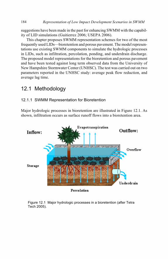
Major hydrologic processes in bioretention are illustrated in Figure 12.1. As shown, infiltration occurs as surface runoff flows into a bioretention area.

Figure 12.1 Major hydrologic processes in a bioretention (after Tetra Tech 2005).


The infiltrated water fills porous spaces in the planting soil mix, and the ex-cess water percolates into the natural soil. The infiltrated water can also discharge downstream through an underdrain pipe, if one is used. During this process, if the inflow rate to the bioretention facility exceeds the infiltration rate to the planting soil, water starts ponding on the ground surface. When the pond-ing depth is exceeded, the excess water becomes overflow. During the dry periods between two events, water held in the planting soil mix leaves the bioretention through percolation to natural soil, the underdrain pipe, and evapotranspiration. The processes of percolation and underdrain drainage stop when the water content of the planting soil mix is equal to the field capacity.

Hydrologic processes illustrated in Figure 12.1 can be grouped into two modules: a planting soil mix module and a ponding area module. The planting soil module determines whether the inflow runoff should be infiltrated by com-paring inflow rate to the infiltration rate of the planting soil. On the basis of the total inflow volume and the planting soil field capacity, the planting soil mix module determines when percolation and underdrain drainage occur, and when these processes stop. It also designates the rate for percolation, underdrain flow and evapotranspiration. The ponding area module determines when the over-flow occurs, the rate of ponding water infiltrating into the planting soil mix, and the evaporation rate.

The behavior of the two bioretention modules (planting soil mix and pond-ing area) described above can be simulated using existing SWMM components. A SWMM representation of the bioretention area that has both modules is shown in Figure 12.2. The representation includes an optional sediment fore-bay, which can be disconnected if not present.

As shown in the schematic, outflow from the sediment forebay is first routed to a flow divider (divider 1), which separates flow to the planting soil mix module and flow to the ponding area module (overflow). The threshold cutoff flow rate for divider 1 is calculated as the bioretention cell surface area multiplied by the planting soil mix infiltration rate; flows up to this rate are routed to the soil mix module, while any remaining increment of flow above this rate is routed to the ponding area module. The planting soil mix module consists of a storage unit (storage unit 1), an overflow orifice (overflow 1), a percolation orifice (percolation 1), and an underdrain orifice (underdrain 1). The ponding area module consists of a storage unit (storage unit 2), an overflow orifice (overflow 2), an orifice that represents ponding water infiltration (infil-tration 1), and a flow divider (divider 2) that separates the infiltrated ponding water between percolation (percolation 2) and underdrain drainage (un-derdrain 2).


Figure 12.2 Schematic for representation of bioretention in SWMM.

Storage unit 1 receives flow routed to the planting soil mix module. The area of storage unit 1 is the same as the bioretention surface area, and the maximum depth (heff) is equal to the effective depth of the planting soil. When the maximum depth of storage unit 1 is exceeded, the excess flow is routed to the ponding area module through an orifice (overflow 1). Percolation to natural soil and underdrain from the planting soil occur only after inflow exceeds the planting soil mix field capacity, which can be expressed as an equivalent depth (hfc) of water in the storage unit. Percolation to the natural soil is assumed to be at a constant rate, which is calculated as the surface area of the bioretention


multiplied by the natural soil infiltration rate. An outlet (percolation 1) with a constant rating curve is used to simulate the percolation, with the height of the outlet being set as hfc. Flow in the underdrain pipe is also simulated using an outlet (Underdrain 1). The rating curve for the underdrain outlet is from an equivalent orifice, and the curve is obtained by setting storage unit 1 with an initial depth of heff and an orifice of the same size as the underdrain pipe at the bottom. After the rating curve table for the equivalent orifice is created, hfc needs to be added to the depth column to ensure that no underdrain occurs be-fore hfc is reached. The height for the underdrain outlet is set as hfc. An evaporation factor is assigned to storage unit 1 to represent the evapotranspira-tion from the bioretention.

Flow that exceeds the planting soil mix infiltration rate is routed to the ponding area module and to storage unit 2, which has the same area as the bioretention. Maximum depth of storage unit 2, or the ponding area, is usually assumed to be 6 in. (0.15 m). When inflow exceeds the storage volume pro-vided by the ponding area, the excess flow is discharged downstream through an orifice (overflow 2). Even though the volume in storage unit 2 represents flow that exceeds the planting soil mix infiltration rate, the ponded water will infiltrate back into the planting soil mix once water starts leaving the bioreten-tion through percolation and underdrain. This happens only after the field capacity of the planting soil mix is exceeded. The infiltration from the ponding area into the planting soil mix is simulated using an orifice (infiltration 1). The diameter of the orifice can be calculated using the following equations:

d = 4aπ

(12.1)

where: d = diameter for the orifice that represents ponding area

infiltration (ft or m), and a = cross-sectional area of the orifice (ft2 or m2).

The cross-sectional area a in Equation 12.1 is calculated as follows:

a = QC 2ghavg

(12.2)

where: Q = infiltration rate from the ponding area into the planting

soil mix (ft3/s or m3/s), C = orifice discharge coefficient, g = constant of gravity, 32.2 ft/s2 (9.81 m/s2), and


havg = average hydraulic head (ft or m).

The infiltration rate Q in Equation 12.2 can be calculated as the surface area of the bioretention multiplied by the planting soil infiltration rate. The average hydraulic head, havg, is calculated as half of the maximum depth in the ponding area, which is usually assumed to be 3 in. (0.08 m).

Because infiltration to planting soil mix from the ponding area should occur only after the field capacity is exceeded, a control rule needs to be specified in SWMM to operate the orifice of Infiltration 1. The rule can be stated as fol-lows:

RULE InfilOrifice1 IF NODE (Storage Unit 1) DEPTH ≥ (hfc) THEN (Infiltration 1) SETTING = 1

RULE InfilOrifice2 IF NODE (Storage Unit 1) DEPTH < (hfc) THEN (Infiltration 1) SETTING = 0

Under the above orifice control rule, infiltration 1 is turned on once the wa-ter depth in storage unit 1 is higher than the depth equivalent to the planting soil mix field capacity (hfc). Infiltration 1 is turned off once the water depth in stor-age unit 1 is lower than hfc due to percolation and underlain drainage.

The infiltrated water from the ponding area is routed to a flow divider (di-vider 2), where the flow is separated for percolation (percolation 2) and underdrain drainage. The percolation rate is the same as the percolation rate at storage unit 1, and the rest of the flow goes to underdrain (underdrain 2). The underdrain flow and the overflow from the ponding area are routed down-stream, and the percolated flow is routed to dummy outfalls for tracking purposes.

12.1.2 SWMM Representation for Porous Pavement

A schematic drawing of major hydrologic processes in porous pavement is shown in Figure 12.3. As rain falls onto porous pavement, the rainfall infiltrates into the porous pavement and then drains through the underlain permeable lay-ers. As the porous spaces in the permeable layers are filled up, water percolates into the natural soil or discharges downstream through an underdrain pipe. Dur-ing this process, surface runoff occurs if the rainfall intensity exceeds the infiltration rate of the porous pavement.


Figure 12.3 Schematic drawing of a simplified porous pavement system (after Tetra Tech 2005).

When representing the porous pavement in SWMM, the multilayer design can be aggregated into an equivalent composite layer, the porous space of which can be simulated using a storage unit. The percolation and underdrain processes can be simulated using approaches that are similar to those in the bioretention. The infiltration rate of the composite layer is a function of the infiltration rate and depth of each permeable layer (Jury et al. 1991), which is stated as follows:

Kcomp =LJ

J=1

N

∑LJKJ

⎛⎝⎜

⎞⎠⎟J=1

N

∑(12.3)

where: Kcomp = infiltration rate for the composite layer (in./h or m/h),

LJ = depth of permeable layer J (in. or m), KJ = infiltration rate for permeable layer J (in./h or m/h),

and N = total number of permeable layers.

A schematic for the porous pavement representation in SWMM is shown in Figure 12.4. As shown, when runoff is routed to the porous pavement, the flow


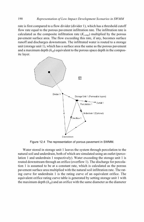
rate is first compared to a flow divider (divider 1), which has a threshold cutoff flow rate equal to the porous pavement infiltration rate. The infiltration rate is calculated as the composite infiltration rate (Kcomp) multiplied by the porous pavement surface area. The flow exceeding this rate, if any, becomes surface runoff and discharges downstream. The infiltrated water is routed to a storage unit (storage unit 1), which has a surface area the same as the porous pavement and a maximum depth (heff) equivalent to the porous space depth in the compos-ite layer.

Figure 12.4 The representation of porous pavement in SWMM.

Water stored in storage unit 1 leaves the system through percolation to the natural soil and underdrain, both of which are simulated using an outlet (perco-lation 1 and underdrain 1 respectively). Water exceeding the storage unit 1 is routed downstream through an orifice (overflow 1). The discharge for percola-tion 1 is assumed to be at a constant rate, which is calculated as the porous pavement surface area multiplied with the natural soil infiltration rate. The rat-ing curve for underdrain 1 is the rating curve of an equivalent orifice. The equivalent orifice rating curve table is generated by setting storage unit 1 with the maximum depth (heff) and an orifice with the same diameter as the diameter


pipe at the bottom. The heights of both percolation 1 and underdrain 1 are set as zero, assuming that the relatively low field capacity of the permeable layers does not affect the start and stop of the percolation and underdrain processes.

12.1.3 Testing of LID Representations

SWMM representations for bioretention and porous pavement were tested against observed data from UNHSC. UNHSC maintains a comprehensive LID monitoring program, through which multiple LIDs are designed, monitored, and analyzed (UNHSC 2007). Long term performances of LIDs, for both aver-age peak-flow reduction and average lag time, are documented in annual reports by UNHSC. Using this data, the SWMM representations of bioretention and porous pavement in this study were tested for these two indicators accord-ingly.

When testing the bioretention and porous pavement representations, the SWMM representation was run for the full 2004–2006 monitoring period (UNHSC 2007). After the simulation was completed, the inflow to and the out-flow from the LIDs for each event were compiled, and the individual peak flow reduction and lag time were calculated. An average peak flow percentage re-duction and an average lag time across the whole simulation period were then calculated. The average values for each LID were compared to the UNHSC-reported values for assessment of the representation schemes.

12.2 Data

Three-year (01/01/2004–12/31/2006) hourly rainfall data were obtained from the nearby Rochester Airport, New Hampshire (COOP ID: 277253). The ob-served annual average evaporation rate from the airport is 0.09 in./d (0.002 3 m/d). The rainfall data were used to generate runoff from a 1 acre parking lot, which is the same as the contributing areas for individual LIDs in the UNHSC experiment lot (UNHSC 2007). The runoff time series were then used as input to the bioretention and porous pavement model representations.

Dimensions for the bioretention facility were obtained from the UNHSC re-port. In the report, the bioretention includes a sediment forebay, which has a capacity of 25% of the water quality volume. The bioretention is 8 ft (2.44 m) wide and 34 ft (10.36 m) long. The planting soil is 30 in. (0.76 m) deep, under-lain with a 12 in. (0.30 m) gravel layer. The field capacity for the sandy loam planting soil mix is assumed to be 0.12 (BCMAFF 2002). A 6 in. (0.15 m) un-derdrain pipe in the gravel layer is used to discharge the infiltrated water


downstream. The underlain natural soil is of the Hydrologic Soils Group (HSG) B, with an infiltration rate of 1.18 in./h (0.03 m/h). The ponding area depth for the bioretention is 6 in. (0.15 m). A summary of the bioretention design is in Table 12.1.

Table 12.1 Design of the bioretention at UNHSC.

Components Design parameters Value Ponding Maximum depth 6 in. (0.15 m)

Depth 30 in. (0.76 m) Porosity 40%

Planting soil mix

Infiltration rate 4 in./h (0.10 m/h) Depth 12 in. (0.30 m) Porosity 40%

Gravel layer

Infiltration rate 14 in./h (0.36 m/h) Orifice Diameter 6 in. (0.15 m)

In the UNHSC design, the porous pavement consists of four layers—a po-rous asphalt layer, a stone choker course layer, a sand filter course layer and a gravel stone layer (UNHSC 2007). A 6 in. (0.15 m) underdrain pipe is placed in the gravel stone layer to discharge infiltrated water. The porous pavement is on an HSG C soil area, and the infiltration rate is 0.20 in./h (0.005 m/h). A sum-mary of the porous pavement design is in Table 12.2.

Table 12.2 Design of the porous pavement at UNHSC.

Components Design parameters Value Depth 4 in. (0.10 m) Porosity 15%

Porous asphalt


Chocker course


Sand filter


Gravel layer

Infiltration rate 14 in./h (0.36 m/h) Orifice Diameter 6 in. (0.15 m)

After the bioretention and porous pavement dimension data were transferred into the SWMM representations, the model was run to evaluate the hydrologic benefits from each LID. The calculation time step for SWMM was set as one minute.


12.3 Results and Discussion

12.3.1 The Bioretention Facility

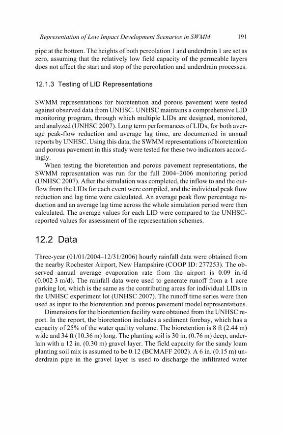
A total of 73 events occurred during the period 01/01/2004—12/31/2006. In-flow to the bioretention representation was compared to the outflow for each of the events over the 3 y period. The peak flow reductions were calculated and plotted in Figure 12.5. The average peak flow percentage reduction is 77%. As a comparison, the UNHSC-reported average bioretention peak flow rate reduc-tion is 82%.

Figure 12.5 Peak flow percentage of reductions for the bioretention representation.

After the 3 y run of the SWMM was completed, the outflow hydrograph from each event was analyzed and the peak flow occurrence time recorded. The outflow peak flow rate occurrence time was then compared to the timing of the peak rainfall intensity and the resulting lag time calculated. Out of the 73 events, 18 events were fully captured by the bioretention and thus had no outflow. The lag times in minutes for the remaining 55 events are plotted in Figure 12.6. The average modeled outflow lag time is 97 minutes, which is close to the UNHSC-reported 92 minutes.


Figure 12.6 Outflow lag time for the bioretention representation.

The bioretention hydrologic performance characteristics are compared with the UNHSC-reported values in Table 12.3. As shown, the long term simulation results from the bioretention representation are close to the UNHSC-observed bioretention performance characteristics.

Table 12.3 Hydrologic performance characteristics of the bioretention representation.

UNHSC report value SWMM represen-tation

Difference

Average peak flow reduction 82% 77% –5%Average lag time (min) 92 97 5

Although the proposed SWMM representation scheme for the bioretention facility has satisfactory results when compared to the observed data, it must be pointed out that the ponding area module of the model representation will bene-fit from additional refinement. In the current scheme (Figure 12.2 above) the infiltrated water from the ponding area is routed to divider 2, where the percola-tion flow is separated and all the rest goes to underdrain flow (underdrain 2). In a more strict representation, the infiltrated flow should be introduced back to


storage unit 1, the water level of which determines the percolation and un-derdrain flow rate from the planting soil cell. However, this approach is not immediately applicable in SWMM, because the introduction of flow from stor-age unit 2 (lower elevation) to storage unit 1 (higher elevation) will inevitably involve the use of a pump and a complex looped configuration.

12.3.2 The Porous Pavement

The porous pavement representation was also run for the 3 y period, and the peak flow reductions from each of the 73 events were calculated and plotted in Figure 12.7. The average peak flow percentage reduction is 77%, in comparison to the UNHSC-reported value of 68%.

Figure 12.7 Peak flow percentage of reductions for the porous pavement representation.

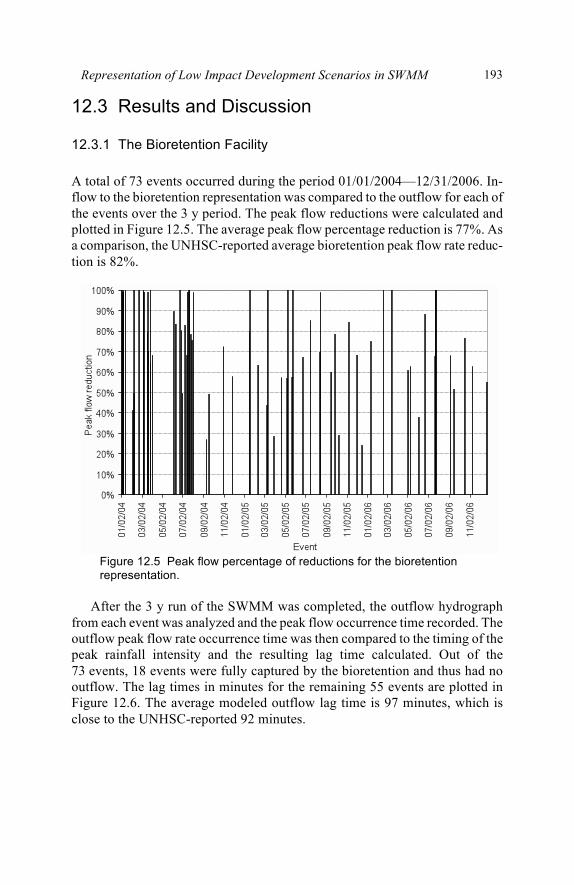
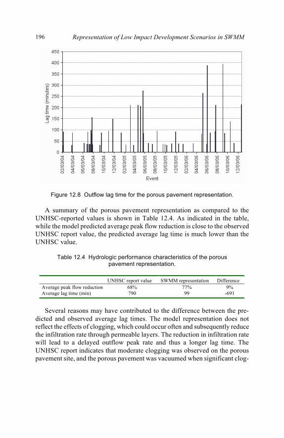
Lag times for the porous pavement representation were calculated for events that had predicted outflow. Out of the 73 events, 50 had outflow in the model simulation. The calculated lag times in minutes for the 50 events are plotted in Figure 12.8. The average modeled lag time is 99 min, in comparison to the UNHSC-reported 790 min.


Figure 12.8 Outflow lag time for the porous pavement representation.

A summary of the porous pavement representation as compared to the UNHSC-reported values is shown in Table 12.4. As indicated in the table, while the model predicted average peak flow reduction is close to the observed UNHSC report value, the predicted average lag time is much lower than the UNHSC value.

Table 12.4 Hydrologic performance characteristics of the porous pavement representation.

UNHSC report value SWMM representation Difference Average peak flow reduction 68% 77% 9% Average lag time (min) 790 99 -691

Several reasons may have contributed to the difference between the pre-dicted and observed average lag times. The model representation does not reflect the effects of clogging, which could occur often and subsequently reduce the infiltration rate through permeable layers. The reduction in infiltration rate will lead to a delayed outflow peak rate and thus a longer lag time. The UNHSC report indicates that moderate clogging was observed on the porous pavement site, and the porous pavement was vacuumed when significant clog-


ging occurred (UNHSC 2007). Clogging also reduces the porosity of the per-meable layers, resulting in less space to store the infiltrated water and decrease in peak flow reduction. The fact that the model representation has a higher av-erage peak flow reduction percentage than the observed value also substantiates this. Another possible reason for the smaller lag time in the model prediction could be related to the assumption that the field capacity of the permeable lay-ers is negligible. If a field capacity value is assigned to the composite layer, no percolation or underdrain will occur before the field capacity is reached. This will delay the occurrence of the outflow peak rate in the model and, thus, in-crease the lag time.

12.4 Conclusions

The SWMM representation schemes for two LIDs, bioretention and porous pavement, were proposed and tested in this study. The proposed representations accounted for the dominant hydrologic processes in each LID, and the represen-tations were based on existing SWMM components. The testing results indicate that the SWMM representation for the bioretention facility resulted in a good match with observed UNHSC data on average peak flow reduction (77% versus the observed 82%) and average lag time (97 min versus the observed 92 min). The representation for porous pavement resulted in a good match with observed UNHSC data on average peak flow reduction (77% versus the observed 68%), but the predicted average lag time (99 min) was much lower than the observed value (790 min). The difference in lag time could be attributed to clogging ef-fects on the site during the data collection period.

In general, the proposed SWMM representations can be used as a basis for evaluating the hydrologic benefits from bioretention and porous pavement im-plementations. In addition, the optional features in the representation schemes provide some flexibility, and can help accommodate variations in LID designs between specific facilities.

Acknowledgments

The authors are grateful for the generous help provided by Dr. Robert Roseen and his research team at the UNHSC. The authors also want to thank the two anonymous reviewers for their thorough and constructive comments that helped to improve this chapter.


References

BCMAFF (British Columbia Ministry of Agriculture, Food, and Fisheries). 2002. Water Conservation Factsheet: Soil Water Storage Capacity and Available Soil Moisture. No. 619.000–1.

Coffman, L.S., R. Goo, and R. Federick. 1999. Low impact development: An innovative alternative approach to stormwater management. In Proc. 26th Water Resources Planning and Management Conference. ASCE, Tempe, AZ.

Elliott, A.H., and S.A. Trowsdale. 2007. A review of models for low impact urban stormwater drainage. Environmental Modeling and Software 22(3): 394–405.

Guitierrez, S. 2006. USEPA’s urban watershed research program in BMPs and restora-tion for water quality improvement. In BMP Technology in Urban Watersheds: Current and Future Directions, 1–17. ASCE Publications, ISBN 0784408726.

Huber, W.C., and L. Cannon. 2002. Modeling non-directly connected impervious areas in dense neighborhoods. In Proc. 9th International Conference on Urban Drainage. ASCE, Portland, OR.

Jury, W.A., W.R. Gardner and W.H. Gardner. 1991. Soil Physics, 5th edition. John Wiley & Sons, New York.

Paul, R.K. 2005. A Milwaukee model for LID hydrologic analysis. In Proc. 2005 Water-shed Management Conference. ASCE, Williamsburg, VA.

Prince George’s County Department of Environmental Resources, Programs and Plan-ning Division. 1999. Low-Impact Development Design Strategies: An Integrated Design Approach. Prince George’s County, MD.

PSAT (Puget Sound Action Team). 2005. Low Impact Development Technical Guidance Manual for Puget Sound. Olympia, WA.

Rossman, L.A. 2008. Stormwater Management Model User’s Manual, Version 5.0. EPA-600-R05-040. Office of Research and Development, USEPA, Cincinnati, OH.

Tetra Tech. 2005. BMP/LID Decision Support System for Watershed-Based Stormwater Management: Users Guide. Prepared for Prince George’s County, Department of En-vironmental Resources, by Tetra Tech, Inc., Fairfax, VA.

UNHSC (University of New Hampshire Stormwater Center). 2007. 2007 Annual Report. University of New Hampshire Stormwater Center, Durham, NH.

USEPA (U.S. Environmental Protection Agency). 2006. BMP Modeling Concepts and Simulation. EPA-600-R06-033. U.S. Environmental Protection Agency, Washington, DC.

representation of low impact development scenarios … · representation of low impact development...

Documents