NBER WORKING PAPER SERIES

REPAIRING A MORTGAGE CRISIS:HOLC LENDING AND ITS IMPACT ON LOCAL HOUSING MARKETS

Charles CourtemancheKenneth A. Snowden

Working Paper 16245http://www.nber.org/papers/w16245

NATIONAL BUREAU OF ECONOMIC RESEARCH1050 Massachusetts Avenue

Cambridge, MA 02138July 2010

Snowden is corresponding author. We thank Price Fishback, Stephen Holland, and seminar participantsat the University of North Carolina Greensboro, the St. Louis Federal Reserve and the 2010 ASSAMeetings for comments and suggestions. We also thank David Cornejo, Diana Liu, Anders Olson,and Spencer Snowden for assistance in assembling the data. All errors are our own. The views expressedherein are those of the authors and do not necessarily reflect the views of the National Bureau of EconomicResearch.

NBER working papers are circulated for discussion and comment purposes. They have not been peer-reviewed or been subject to the review by the NBER Board of Directors that accompanies officialNBER publications.

© 2010 by Charles Courtemanche and Kenneth A. Snowden. All rights reserved. Short sections oftext, not to exceed two paragraphs, may be quoted without explicit permission provided that full credit,including © notice, is given to the source.

Repairing a Mortgage Crisis: HOLC Lending and its Impact on Local Housing MarketsCharles Courtemanche and Kenneth A. SnowdenNBER Working Paper No. 16245July 2010JEL No. E44,G01,G18,G21,G22,G28,N22,N62,N92,R31,R51

ABSTRACT

The Home Owners’ Loan Corporation purchased more than a million delinquent mortgages from privatelenders between 1933 and 1936 and refinanced the loans for the borrowers. Its primary goal was tobreak the cycle of foreclosure, forced property sales and decreases in home values that was affectinglocal housing markets throughout the nation. We find that HOLC loans were targeted at local (county-level)housing markets that had experienced severe distress and that the intervention increased 1940 medianhome values and homeownership rates, but not new home building.

Charles CourtemancheBryan School of Business and EconomicsP.O. Box 26165University of North Carolina at GreensboroGreensboro, NC 27402cjcourte@uncg.edu

Kenneth A. SnowdenBryan School of Business and EconomicsP.O. Box 26165University of North Carolina at GreensboroGreensboro, NC 27402and NBERsnowden@uncg.edu

1

REPAIRING A MORTGAGE CRISIS:

HOLC LENDING AND ITS IMPACT ON LOCAL HOUSING MARKETS

Abstract

The Home Owners‘ Loan Corporation purchased more than a million delinquent mortgages

from private lenders between 1933 and 1936 and refinanced the loans for the borrowers.

Its primary goal was to break the cycle of foreclosure, forced property sales and decreases

in home values that was affecting local housing markets throughout the nation. We find

that HOLC loans were targeted at local (county-level) housing markets that had

experienced severe distress and that the intervention increased 1940 median home values

and homeownership rates, but not new home building.

―[A] tremendous surge of residential building in the [last] decade…was matched by an ever-

increasing supply of homes sold on easy terms [and only]… a small decline in prices was

necessary to wipe out this equity. Unfortunately, deflationary processes are never satisfied with

small declines in values. They feed upon themselves and produce results out of all proportion

to their causes… In the field of real-estate finance, particularly, we have depended so much

upon credit that our whole value structure can be thrown out of balance by relatively slight

shocks. When such a delicate structure is once disorganized, it is a tremendous task to get it

into a position where it can again function normally.‖ (Hoagland, 1935)

Introduction

Between 1929 and 1933 hundreds of thousands of homeowners defaulted on mortgages,

thousands of mortgage lending institutions failed, and surviving mortgage lenders dramatically curtailed

their lending operations. Observers of events since 2007 will find striking parallels in the background and

character of the housing and mortgage crisis of the 1930s. That episode also followed a decade of rapid

growth and innovation in the residential mortgage market that quickly reversed into a self-reinforcing

cycle of loan delinquency, foreclosure, forced property sales and decreases in home values.1 Henry

Hoagland was well-positioned to characterize the crisis as a member of the Federal Home Loan Bank

1 See Wheelock (2008) for an overview of the housing boom of the 1920s and crisis in the 1930s.

2

Board. The FHLBB supervised most depression-era housing programs including the Home Owners‘

Loan Corporation which was in the midst of refinancing about one million delinquent mortgages when

Hoagland penned his observations in 1935. All of these distressed loans were held by private mortgage

lenders before HOLC purchased and refinanced them, so the program provided assistance not only to

homeowners but also to a severely disrupted mortgage market. By 1936 HOLC held mortgage loans on 1

out of every 10 nonfarm owner-occupied home in the U.S. and held nearly 20 percent of the nation‘s

home mortgage debt.

Because it combined the purchase of distressed mortgages with a loan modification program, the

HOLC could have ameliorated the impacts of the 1930s crisis through three different channels.2 First, by

refinancing so many distressed loans it immediately reduced the number of home foreclosures and

moderated the cycle of forced home sales, lower housing prices and additional foreclosures. Second,

HOLC continued to reduce the number of foreclosures after its lending operations ended in 1936 by

adopting generous servicing and work-out policies (Harriss, 1951, 64-70).3 Finally, HOLC strengthened

the balance sheet of private home lending agencies by substituting liquid, low-risk, government-insured

bonds for delinquent mortgages so that they could be more patient servicers of their remaining loans and

resume new mortgage lending activities.4

2 HOLC is an interesting case study for observers of the recent mortgage crisis because it combined purchases of

toxic mortgages with loan modifications. During the recent crisis, in contrast, programs have been designed to

perform only one of these functions. Toxic mortgage loans, for example, were supposed to have been purchased by

the Troubled Assert Relief Program (TARP) and the Public-Private Investment Program (PPIP). Loan modification

programs, on the other hand, have included the White House/Treasury HAMP and HARP programs, the FDIC‘s

IndyMac Loan Modification program and Federal Housing Finance Agency‗s program to modify loans held by

FannieMae or FreddieMac.

3 Harriss (1951, 64-71) describes HOLC‘s loan servicing model which included postponement of principal payments

for the first three years and extensive personal contact and counseling if the loan became delinquent. HOLC,

nonetheless, foreclosed on 20 percent of its loans.

4 HOLC paid for mortgages with its own bonds on which both principal and interest were guaranteed by early 1934

and for which a broad secondary market developed. HOLC bonds paid low interest rates (3 or 4 percent) relative to

mortgages, but they were replacing delinquent mortgages in investors‘ portfolios.

3

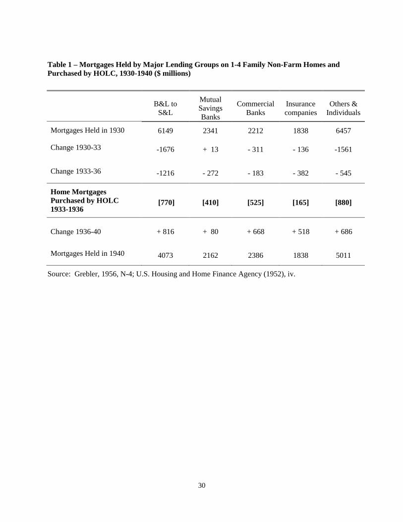
Table 1 provides a broad overview of the disruptions in the residential mortgage market during

the 1930s and the magnitude and scope of HOLC activities against that backdrop. Between 1930 and

1933 privately-held mortgage debt on 1-4 family nonfarm homes contracted by $3.6 billion or about 19

percent of the total. The bulk of the decrease occurred in the portfolios of Building & Loans and

individual investors which were the two investor groups most heavily connected to innovation and growth

within the residential of mortgage market during the 1920s. 5 Over the next three years privately held

mortgage debt fell by another 17 percent and, as be seen in the third and fourth rows of Table 1, HOLC

purchases represented nearly two-thirds of the decrease for Building & Loans and more than the total

decrease for individual investors, mutual savings banks and commercial banks. The payments lenders

received from these transactions, moreover, were sufficient to fund more than 80 percent of the

subsequent increase in mortgage holdings between 1936 and 1940 for each lending group except

insurance companies.

[INSERT TABLE 1 ABOUT HERE.]

HOLC loan purchases were substantial in magnitude and widely distributed, but privately held

home mortgage debt still decreased by 20 percent between 1930 and 1940 while nonfarm homeownership

fell from 46 percent to 41 percent and the median value of nonfarm homes decreased by 37 percent. But

even though HOLC did not reverse all of the damage from the crisis, its lending and purchase programs

might have mitigated the impacts if they were well-targeted and effective. We explore that possibility in

this paper. After briefly discussing the literature on the HOLC, we examine county-level rates of HOLC

applications, approvals and loans and find that they were all related to indicators of economic and housing

distress as well as other demographic, economic and political characteristics. Among these other

5 Difficulties that persisted throughout the decade includes the foreclosed real estate accounts of Massachusetts

mutual savings banks which still represented two-thirds of their capital surplus in 1940, the liquidation of 1920s

securitization structures that occupied state and federal regulators into the early 1940s and the Building & Loan

which lost 3,000 associations after 1933 and still held 12 percent of its assets in real estate in 1940. See Lintner

(1948, 272) for the mutual savings banks, Snowden (2003) for the B&L industry and Snowden (2010) for the failure

of the mortgage guarantee companies and real estate bond houses during the 1930s.

4

influences was the distance between the county and the nearest HOLC office which indicates,

unsurprisingly, that residential mortgage markets were still spatially segmented by information and

transaction costs in the 1930s.6 Based on this evidence, we exploit the spatial configuration of the HOLC

program to identify the impacts of HOLC lending on home values and homeownership rates in 1940, and

on new housing construction in 1935-1940. We find that HOLC lending boosted home values and

homeownership rates during the second half of the 1930s, but that the program did not stimulate new

home construction.

Background and Literature on HOLC

HOLC was a remarkable federal initiative in at least two respects. First, the agency organized and

began to operate a truly national mortgage loan origination network just a few months after being created

in the summer of 1933. Second, the corporation dissolved as originally intended in 1951 after it had

finished servicing the loan portfolio that it had created between 1933 and 1936. Harriss (1951) describes

HOLC procedures, operations and structure over this entire life span and his account remains the

indispensable reference for any analysis of the agency.7 To gain insights about the program‘s operation

and effectiveness, however, Harriss‘s largely descriptive account needs to be supplemented with

systematic examination of three issues: the factors which determined participation by homeowners and

lenders in the HOLC program, the forces which shaped the allocation of HOLC loan purchases and

refinancing across the nation‘s markets, and the program‘s impact on local and national housing market

outcomes. In this paper we make contributions along all three fronts.8

By name and legislative intent HOLC was first and foremost a program designed to assist

distressed homeowners, but no one has yet systematically examined why nearly two million households

6 Snowden (1997, 2003) documents spatial segmentation in the residential mortgage market before 1930.

7 Tough (1951) also provides an important view of the ultimate success of HOLC at the program‘s end.

8 The research employs newly digitized county-level data on number of HOLC applications and acceptances (from

U.S. Federal Home Loan Bank Board 1937 Annual Report) and the number of homes built in four quinquennia:

1920-24, 1925-29, 1930-35 and 1935-40 (from 1940 U.S. Census of Housing).

5

applied to HOLC for mortgage relief between 1933 and 1936.9 We do so and find that variation in HOLC

application rates across counties reflected, most importantly, the structure of local housing markets and

the distress felt within them. We take this as evidence that the program successfully attracted applicants

who were in need of loan modification rather than individuals seeking general economic relief.

We also examine the determinants of the rate at which these applications were accepted into the

program. Rose (2009) has examined the issue for a sample of individual HOLC loans made in New

York, New Jersey and Connecticut with a focus on the terms that the agency offered to lenders in its role

as a ―bad bank‖.10

He shows that the agency set appraisals, loan balances and loan prices above the levels

warranted by current property values in order to encourage the participation of lenders by reducing the

losses on loan sales that they had to write down.11

Rose‘s work establishes that HOLC acceptance rates

were determined by the interaction of several factors—the program‘s eligibility requirements, staff

judgments regarding borrower need and property value, and the negotiating strength of lenders. We assess

the net impact of all of these by examining the determinants of county-level acceptance rates into the

program. We find that the pattern of acceptance at this level of aggregation was closely associated with

local housing characteristics and measures of distress that should have mattered in a targeted mortgage

relief program.

Our measure of HOLC loan activity—the percentage of 1930 nonfarm households in each county

that received HOLC refinancing—is the product of the loan application and acceptance rates and so was

determined by similar influences. In the second section we estimate the impact that HOLC intervention

had on three outcomes in local housing markets—home values and homeownership rates in 1940 and the

9 Harriss (1951, 16-23) provides a descriptive account for HOLC applicants in the aggregate.

10 See Ergungor (2007) and Bernanke (2009) for discussions of modern versions of ―bad banks‖ to purchase toxic

assets in Sweden, Peru and other countries during crises.

11 Under HOLC procedures the higher appraisals also increased the amounts borrowers had to refinance on their

HOLC loans. Rose‘s work clarifies, therefore, that HOLC faced a tradeoff by serving both sides of the mortgage

transaction—actions and policies that generated greater lender participation also raised the delinquency rate on

HOLC‘s own loan portfolio.

6

number of new homes built in each county between 1935 and 1940. We chose these measures to assess

the program‘s impact on goals that were emphasized in legislation and contemporary discussion—

preserving homeownership, stabilizing home values and stimulating a recovery in residential construction

activity. The distinction among the three is important because other major New Deal housing programs,

most notably the FHA mortgage insurance program, were specifically designed to stimulate home

building. Taken in this light our findings reveal an interesting and revealing pattern—HOLC loan activity

increased home values and homeownership rates in 1940, but not residential construction.

In concurrent work Fishback, Lagunes, Horrace, Kantor, and Treber (2010) (henceforth FLHKT)

also examine the impact of HOLC lending and find that it had positive effects on home values and the

stocks of owned and rented homes in the 2,463 counties with 1930 populations below 50,000. We also

find HOLC impacts on home values and ownership for a restricted sample of counties, but in our case this

includes counties (more than 2,730) that did not contain an HOLC loan office. In the next-to-last section

we examine the differences in the methods we and FLHKT used and, more importantly, differences in the

interpretations of the results. FLHKT conjecture that HOLC intervention was more effective in smaller,

less populated counties because the institutional structure of mortgage markets was thinner in these areas

than in larger cities. We argue, in contrast, that the ―distance-from-HOLC office‖ instrument that is used

in both papers to identify treatment effects is an effective instrument only outside the relatively large

counties in which HOLC offices were located. Our view, therefore, is that the impact of HOLC within

the nation‘s largest urban markets remains an important, but open, issue.

The story of HOLC complements other literature that has shown that disruptions in credit markets

contributed to both the depth and length of the Great Depression. Mishkin (1979) attributes the dramatic

fall in consumption spending in the early 1930s to the negative impacts that decreases in stock values and

home prices, and increases in the real burden of debt, had on household balance sheets. HOLC was

designed to ameliorate the housing market shocks that Mishkin examined, but also the disruptions

associated with foreclosure that his analysis did not address. Bernanke (1983), on the other hand,

establishes context for the second side of the HOLC story—the impact the agency had on mortgage

7

lending institutions. Bernanke showed that an index of bank failure, which he uses to proxy for the ―cost

of credit intermediation,‖ helps to explain the severity of the decline in real output during the 1930s. No

segment of the nation‘s financial structure suffered greater damage during the 1930s than the mortgage

market. Taken in this light, Bernanke‘s argument provides good reason to view HOLC as an attempt to

repair credit channels. We conclude that it did.

Allocation of HOLC Loans across Counties

In its Fifth Annual Report in 1937, the Federal Home Loan Bank Board reported the number of

HOLC loans applied for and the number made for each county between 1933 and 1936. Scaling these

numbers by the number of occupied and owner-occupied nonfarm housing units as measured in the

Census of 1930, we construct four measures of HOLC loan activity: 1) the number of HOLC applications

in each county as a percentage of owner-occupied nonfarm homes in 1930 (application rate), 2) the

percentage of HOLC applications accepted for purchase and refinancing (acceptance rate), 3) the number

of homes refinanced by HOLC as a percentage of the number of owner-occupied homes in 1930 (loan

rate 1), and 4) the number refinanced as a percentage of all nonfarm homes in 1930 (loan rate 2). The

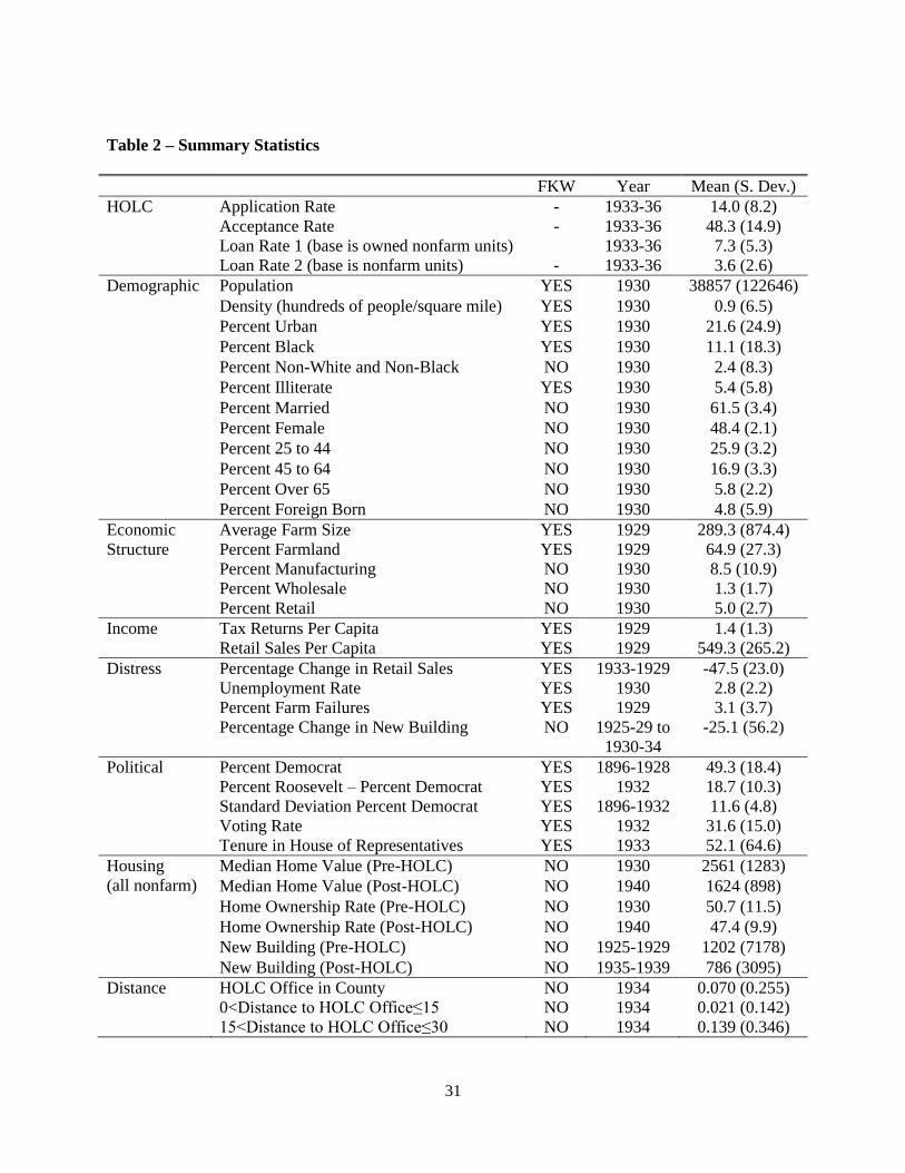
first panel of Table 2 shows that fourteen percent of owner-occupied households in the average county

applied for HOLC loans, that an average of just under fifty percent of applications were accepted, and that

HOLC financed an average of just over 7 percent of owned homes, or 3.6 percent of all nonfarm homes.12

[INSERT TABLE 2 ABOUT HERE.]

We examine county-level variation in application, acceptance and loan rates in this section to

gain insight into the characteristics of borrowers who applied for HOLC relief, the factors that were

associated with HOLC loan approval and the considerations that explained the pattern of HOLC activity

across local housing markets. The overall HOLC loan rate for each county is simply the product of the

application and acceptance rates, so we focus on the latter two first.

12

Harriss (1951, 21) approximates application rates as percentages of estimates of owner-occupied, mortgaged

homes in each state, but he admits the estimates are crude because they rely on patterns of mortgage drawn from the

1940 Census of Housing.

8

HOLC mortgages dominated refinancing alternatives available from private lenders in 1933

because the agency‘s loans were offered on relatively generous terms and were readily available for

eligible borrowers. The HOLC loan rate, for example, was 5 percent when prevailing rates in the private

market were six percent and higher.13

The agency could also lend up to 80 percent of generously

appraised home values for a term of fifteen year terms with full amortization of principal. HOLC helped

popularize the familiar modern mortgage contract, in fact, at a time when the contractual structure of the

mortgages that had financed the housing boom of the 1920s contributed to severe disruptions and

rationing in the private mortgage market. Many homeowners, for example, were forced to find new

lenders in the early 1930s who would refinance short-term, straight mortgage loans on which only interest

had been paid up to that point; many other borrowers lost equity they had accumulated in Building &

Loan shares that served as a sinking fund to pay off the loans they had taken out from these institutions.14

So by 1933 hundreds of thousands of mortgagors sought refinancing or renegotiation on existing

mortgage loans at the same time thousands of private lending institutions had failed and surviving

mortgage lenders were severely curtailing their lending operations.

In this environment Harriss (1951, 22) estimates that 40 percent of the nation‘s home mortgage

borrowers applied for HOLC loans; given the generous terms offered by the agency it is perhaps

surprising that even greater numbers did not apply. The demand for HOLC loans was restricted,

however, by eligibility requirements that should have controlled whether a loan application was approved

and, therefore, the number and types of borrowers who would have found it worthwhile to apply.15

The

program was designed to serve only nonfarm owners of 1-to-4 family residential property who had

13

Volume II of the reports from the 1932 President‘s Report on Homeownership provides an extensive discussion of

loan terms available in the private mortgage market. See Gries and Ford, 1932, 52-97.

14 Snowden (2003) describes the fragility of the traditional share accumulation loan used by B&Ls during the 1930s

mortgage crisis.

15 See Rose (2009) for an examination of the HOLC acceptance decision at the individual loan level for a sample of

loans that the agency made in New York, New Jersey and Connecticut. He focuses on how HOLC used the

appraisal decision to elicit lender‘s willingness to sell their loans.

9

become delinquent on an existing mortgage. HOLC loans were also restricted in size: to no more than 80

percent of the property‘s appraised value, to amounts of not more than $14,000, and to property that was

valued at no more than $20,000. In addition, the applicant had to establish that she had been unable to

refinance with a private lender, that she was financially capable of fulfilling the terms of the HOLC loan

and that her property was sufficiently valuable to leave the agency whole if she did not.

HOLC was not designed to be a general relief program, therefore, but to serve as a temporary,

targeted intervention to fill gaps in a severely disrupted private mortgage market. To determine whether

this mission actually shaped the character of loan applications and the patterns of loan approval, we

employ a modified version of the empirical model that Fishback, Kantor and Wallis (2003) (henceforth

FKW) used to examine variations in county-level per capita spending levels for 20 New Deal grant and

loan programs, including HOLC. FKW were particularly concerned in assessing whether the variation in

spending levels across localities was associated strictly with the need for relief, recovery and reform, or

whether political considerations were also at work. To measure these influences they included

demographic controls (population, density, urban, race and literacy), measures of economic structure and

income (importance and size of farms, and per capita levels of tax returns and retail sales), proxies for

distress (unemployment in 1930 and farm failures and the change in retail sales between 1929 and 1933),

and a rich set of political variables.16

We augment their model with a number of additional independent variables in an effort to build a

model specifically tailored to HOLC as opposed to New Deal programs in general. We add to the set of

demographic characteristics variables representing age, gender, marital status and nativity, all of which

should have influenced the rate and method of financing homeownership. We then add to the set of

economic structure variables the share of gainful workers employed in manufacturing, retail and

wholesale establishments to provide a fuller picture of the makeup of the nonfarm economy in each

16

We thank FKW for the use of their political variables, retail sales and tax return measures. We omit their

committee chair political variables, as we were unable to find a clear connection between them and any of our

dependent variables.

10

county.17

Perhaps most importantly, we add to the set of distress variables a county-level measure of

housing market distress—the percentage change between 1925-1929 and 1930-1934 in the number of

nonfarm dwelling units built.18

We consider this a key measure of disruption in local housing and

mortgage markets that should have influenced the perceived need for HOLC refinancing among

borrowers and the judgments of HOLC administrators about that need.

We also build on FKW‘s model by including a set of additional housing market variables to

capture factors that should have influenced eligibility for HOLC refinancing and, therefore, both

application and acceptance rates. First and foremost, the property already had to be encumbered to be

considered for an HOLC loan. Some of the demographic variables—such as population, density, and the

proportion of the population that was urban and middle-aged—should proxy for access to mortgage

finance within the county prior to the crisis. To these we add the natural logarithms of nonfarm median

home values in 1930 and the number of new homes built between 1925 and 1929 since newer and higher-

priced homes were more likely to have already been encumbered by 1930. High-priced homes of recent

vintage should also have appraised for greater property values in 1933, so these same two variables could

have been associated with higher acceptance as well as application rates. We also include the nonfarm

homeownership rate in each county to see if loan applications or acceptances were sensitive to the mix of

owned and rented housing in the local market.19

Finally, we add distance from the nearest HOLC office location to our specification to reflect one

of HOLC‘s most impressive accomplishments—in a matter of months the agency created a loan

origination and servicing network that was truly national in scope. HOLC had opened more than 200

17

The demographic and economic structure variables were taken from ICPSR data set 2896.

18 The 1930 and 1940 median nonfarm home values are taken from ICPSR data set 2896. The number of nonfarm

housing units built in each county between 1925-1929, 1930-1934 and 1935-1940 were taken from the self-reported

―vintage‖ data for the housing stock that was reported in Volume II of the 1940 Census of Housing of 1940.

19 The application rate and loan rate 1 dependent variables already incorporate the county‘s homeownership rates by

construction, so we add the homeownership rate to the model to assess if local tenure patterns had an impact other

than arithmetic on application and acceptance rates.

11

offices by 1934, with at least one in every state.20

Office location mattered for HOLC lending volume

because distance increased the costs of mortgage lending for both borrowers and the agency—appraisals

required onsite inspections and mortgage applications and documents had to move among homeowners,

county officials and HOLC staff. We include an indicator for counties containing an HOLC office,

another for counties located within 15 miles of an office but not containing an office, and a third for

counties located between 15 and 30 miles away from the nearest office. The omitted base category is a

distance of greater than 30 miles.21

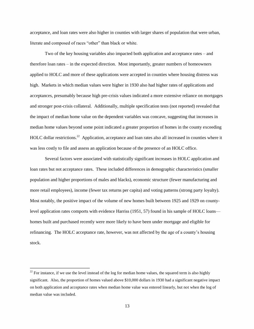
Our model, therefore, includes seven sets of regressors and takes the following form:

where i and s index counties and states. HOLC represents either loan rate, application rate, or acceptance

rate. DEMO, ECON, INC, DISTRESS, POL, and HOUS are the sets of demographic, economic

structure, income, distress, political, and housing variables. OFFICE includes the variable for whether

there was an HOLC office in the county as well as the two distance variables. Following FKW, we

include state fixed effects, denoted by . Table 2 provides descriptive statistics for variables in each of

these categories, along with information on whether they were included in FKW‘s model.

20

The location of HOLC offices in 1934 were taken from Federal Home Loan Bank Board (1934) which provides

the location of all HOLC offices on January 15, 1934 by which time 880,000 applications, or more than 40 percent

of the 1933-35 total, had been filed. At this time FHLB reported 301 offices, of which 79 were listed as agencies,

sub-district offices or wholesale operations offices. For this paper we defined HOLC offices to be only the 48 state

offices and 174 district offices open as of January 1934—these combine into 209 counties which contained an

HOLC office in our sample. HOLC continued to open offices and by November 1934 there were a total of 458

offices at which HOLC applications could be filed. The number of offices fell beyond this point (Harriss, 140).

21 We measure distance between the center of each county and the city in which nearest HOLC office was located.

We considered alternative distance specifications but found no evidence that additional distance impacted HOLC

loan rate beyond 30 miles. Within the 30 mile range, we chose 15-mile groupings of counties because these

distances maximize the F statistic from a test of joint significance of the office variables.

12

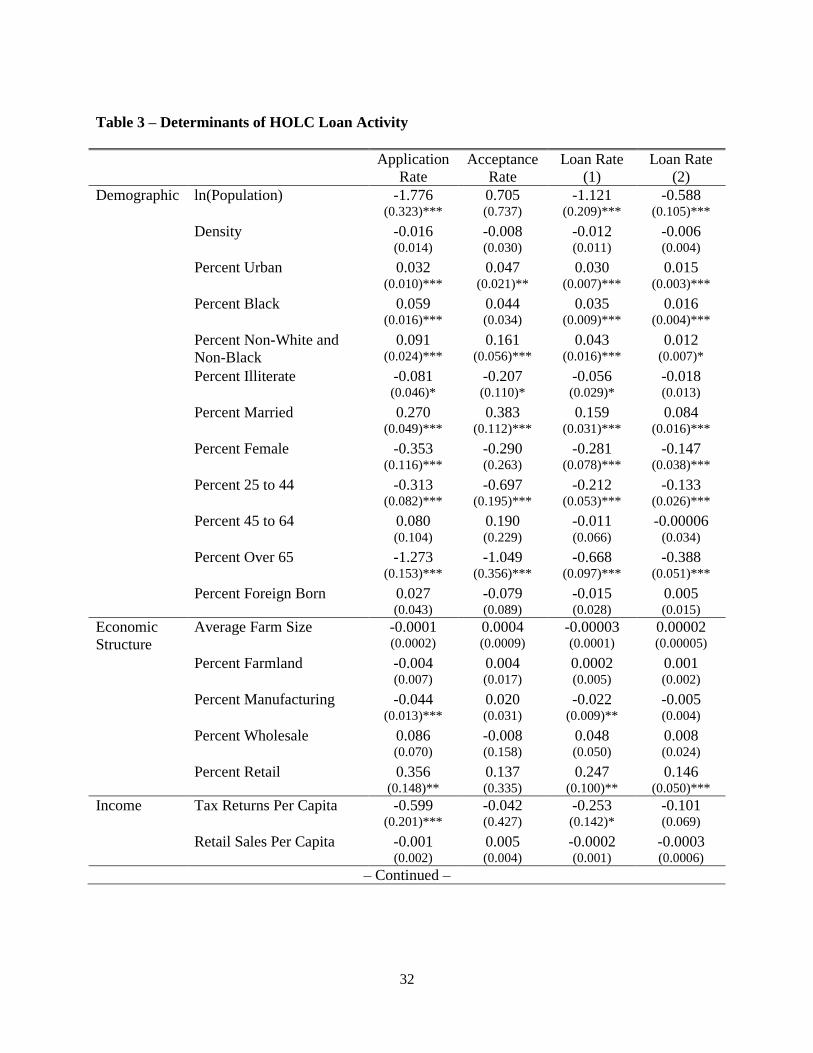
A comparison of the results for the application and acceptance regressions (see columns 1 and 2

of Table 3) reveals interesting patterns about the broad set of factors that were at work in the interactions

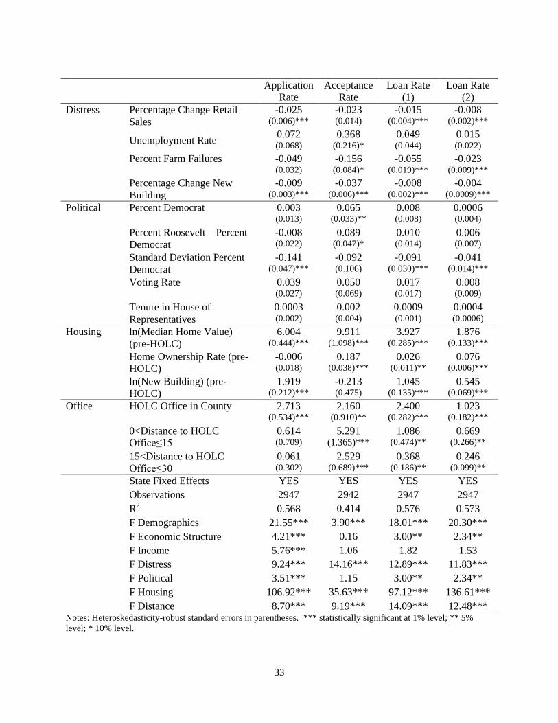
among borrowers, lenders and the HOLC staff. The bottom rows of Table 3 report F-statistics for the

joint significance of the different categories of independent variables. The demographic, economic

structure, income and political variables explain more of the variation in application rates than in

acceptance rates across local housing markets. The distress, housing and distance variables taken as

groups, on the other hand, explain substantial variation in the rate at which applications were both filed

and accepted. These latter groups of variables have been chosen to reflect the structure of local housing

markets, and the distress and lending costs within them. The importance of these influences as a group

provides evidence that HOLC staff, borrowers and lenders all understood the goals and limits on HOLC

as a targeted housing program.

The third and fourth columns of Table 3 report the regression results for the number of HOLC

loans as a percentage of owner-occupied homes (loan rate 1) and a percentage of all nonfarm homes (loan

rate 2). The former is simply the product of the application and acceptance rates in each county so these

results provide a useful representation of the impacts of specific variables on application and acceptance

rates. The latter is the best measure of the overall extent of HOLC treatment in the county and will

therefore be important when examining impacts in the next section. We can partition the factors that

influenced variations in overall HOLC loan activity across counties into three groups: those that only had

a statistically significant effect on application rates, those that only had a significant effect on acceptance

rates and those had significant effects on both. We begin the discussion with the last group.

Marital status and middle-age were associated with both higher application and acceptance rates –

and therefore loan rates – in our national sample of counties just as Harriss (1951, 51-2) found for a

sample of HOLC loans made in New York, New Jersey and Connecticut. His explanation was that

middle-aged heads of households applied to HOLC in greater numbers because they were more likely to

have outstanding mortgages than younger, older or single persons. They were also more likely to be

approved for the loan because they had relatively steady employment and income. Application,

13

acceptance, and loan rates were also higher in counties with larger shares of population that were urban,

literate and composed of races ―other‖ than black or white.

Two of the key housing variables also impacted both application and acceptance rates – and

therefore loan rates – in the expected direction. Most importantly, greater numbers of homeowners

applied to HOLC and more of these applications were accepted in counties where housing distress was

high. Markets in which median values were higher in 1930 also had higher rates of applications and

acceptances, presumably because high pre-crisis values indicated a more extensive reliance on mortgages

and stronger post-crisis collateral. Additionally, multiple specification tests (not reported) revealed that

the impact of median home value on the dependent variables was concave, suggesting that increases in

median home values beyond some point indicated a greater proportion of homes in the county exceeding

HOLC dollar restrictions.22

Application, acceptance and loan rates also all increased in counties where it

was less costly to file and assess an application because of the presence of an HOLC office.

Several factors were associated with statistically significant increases in HOLC application and

loan rates but not acceptance rates. These included differences in demographic characteristics (smaller

population and higher proportions of males and blacks), economic structure (fewer manufacturing and

more retail employees), income (fewer tax returns per capita) and voting patterns (strong party loyalty).

Most notably, the positive impact of the volume of new homes built between 1925 and 1929 on county-

level application rates comports with evidence Harriss (1951, 57) found in his sample of HOLC loans—

homes built and purchased recently were more likely to have been under mortgage and eligible for

refinancing. The HOLC acceptance rate, however, was not affected by the age of a county‘s housing

stock.

22

For instance, if we use the level instead of the log for median home values, the squared term is also highly

significant. Also, the proportion of homes valued above $10,000 dollars in 1930 had a significant negative impact

on both application and acceptance rates when median home value was entered linearly, but not when the log of

median value was included.

14

Two variables that reflect policies implemented by HOLC staff had statistically significant effects

on acceptance and loan rates but not application rates. Applications were approved at lower rates in

counties with high number of farm failures because HOLC staff was instructed to transfer applications

from farmers to the Farm Credit Administration (Harriss, 24). Applications were accepted with greater

frequency in markets with higher rates of homeownership, consistent with Harriss‘ observation (1951, 51)

that HOLC viewed properties located in settled, established residential areas more favorably than those in

mixed, transitional neighborhoods.

Three other variables were weakly associated with higher acceptance rates, but had no significant

impact on overall HOLC loan rates or application rates: the unemployment rate in 1930 and higher shares

of Democratic and Roosevelt votes in 1932. We take this as evidence that HOLC was successful in not

becoming either a general relief program or an instrument of patronage. Note as well that the political

variables as a group explain small shares of the overall variability in either the application or acceptance

rate (refer to the F-stats).

We close the discussion of HOLC allocations by focusing on the results for the HOLC office

variables separately, as they will prove crucial to the identification of HOLC‘s impacts in the next section.

Having an HOLC office increases a county‘s application, acceptance and loan rates. Interestingly,

though, the nearest HOLC office being outside the county but less than 15 miles away or between 15 and

30 miles away had a strong impact on acceptance and loan rate but not application rate.23

This result is

important and interesting for two reasons. First, it indicates that spatial segmentation in the mortgage

market of lending operated more through supply than demand—the costs to HOLC of on-site appraisals

and filing loan documents were greater for loans that were made in more distant counties. Second, the

23

Note also the non-monotonic relationship between distance and acceptance rates: counties within 15 miles of the

nearest HOLC office actually had a higher acceptance rate ceteris paribus than counties containing an HOLC office.

One possible explanation is that, because of the higher application rates in counties with an HOLC office, these

applications were on average weaker than those from surrounding counties, leading to more rejections.

15

impact that these costs had on HOLC treatment levels is plausibly exogenous and provides an avenue

through which we can identify the impacts of HOLC loan activity on local housing outcomes.

HOLC’s Impacts on Local Housing Markets

We next turn to an evaluation of the effectiveness of HOLC intervention in stabilizing the

housing market. An OLS estimator of the relationship between percentage of homes refinanced by

HOLC and housing market outcomes would likely be biased downward since HOLC loans were

distributed disproportionately to areas facing the greatest housing market and overall distress, as shown in

the preceding section. We therefore estimate HOLC‘s impact with two-stage instrumental variables

models in which the first stage predicts HOLC treatment intensity using an equation similar to (1) and the

second examines the relationship between treatment intensity and 1940 non-farm home values and

ownership rates, as well as new non-farm housing units from 1935 to 1940. Identification requires one or

more regressors from (1) that can be excluded from the second stage, meaning that, conditional on the

controls, they must only be correlated with post-HOLC home values, ownership rates, and new building

through their effect on HOLC treatment. Of the independent variables that strongly predicted loan rates

in the preceding section, the three HOLC office variables – whether the nearest HOLC office was located

in the county, outside the county but less than 15 miles away, or 15 to 30 miles away – are the most

plausible candidates to satisfy such an exclusion restriction.

However, the non-random nature of HOLC office locations poses a potential problem for such an

identification strategy: offices may have been placed in areas facing the greatest housing market distress.

This could have occurred for two distinct reasons. First, HOLC administrators generally placed offices in

large cities, and it appears that the Great Depression impacted housing markets in large cities more

severely than in other areas. Specifically, the correlation between county population in 1930 and our

measure of housing market distress – percentage change in new building between 1925-29 and 1930-34 –

is a highly significant -0.25. Second, conditional on population HOLC administrators could have

16

intentionally placed offices in the most distressed areas in an effort to best meet the needs of homeowners

and lenders. These phenomena may lead to a downward bias if all three office variables are used as

instruments. The controls for population, population density, percent urban, distress and 1930 housing

market conditions would mitigate the extent of the bias but may not eliminate it completely.

Fortunately, our indicator of nonfarm housing market distress – percentage change in new

building during the early stages of the depression – allows us to test whether HOLC offices were indeed

placed in areas in which housing markets were the most troubled. We begin by computing correlations

between percentage change in new building from 1925-29 to 1930-34 and each of the three distance from

HOLC office variables. The correlation between percentage change in new building and whether the

county contains an office is -0.22 and significant at the 0.01 percent level. This strong relationship is not

surprising given the preceding discussion. Interestingly, though, the correlations for the other two office

variables are much smaller. The correlation between percentage change in new building and whether the

nearest office is outside the county but less than 15 miles away is -0.04 and significant at only the 5

percent level despite the large sample. The correlation between percentage change in new building and

whether the nearest office is 15 to 30 miles away is a statistically insignificant -0.01.

In Figure 1 we display kernel density functions for percentage change in new building, stratified

by nearest HOLC office location. These plots reveal a similar story. The kernel density function for

counties with an office lies well to the left of the function for the ―control group‖ of counties whose

nearest office is more than 30 miles away. The kernel density functions for counties whose nearest office

is less than 15 miles away and those whose nearest office is 15 to 30 miles away, however, are similar to

that of the control group in shape and value at which the function is maximized.24

The correlations and

kernel density plots therefore suggest that HOLC offices were indeed located in counties facing the most

housing market distress, but that the degree to which this relationship spilled over into surrounding areas

was minimal. Consequently, the under 15 and 15-30 mile groups are the most appropriate comparison

24

The kernel density functions for these groups are less smooth and have a narrower range than the kernel density

function of the control group, but this is likely because the control group is much larger (2,373 counties).

17

groups for the over 30 mile control group, while the counties containing an office form a less appropriate

comparison group.

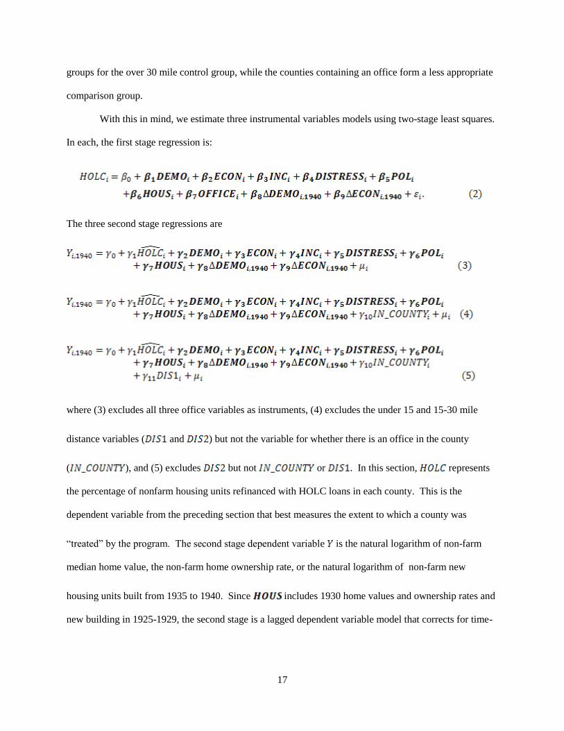
With this in mind, we estimate three instrumental variables models using two-stage least squares.

In each, the first stage regression is:

The three second stage regressions are

where (3) excludes all three office variables as instruments, (4) excludes the under 15 and 15-30 mile

distance variables ( and ) but not the variable for whether there is an office in the county

( ), and (5) excludes but not or . In this section, represents

the percentage of nonfarm housing units refinanced with HOLC loans in each county. This is the

dependent variable from the preceding section that best measures the extent to which a county was

―treated‖ by the program. The second stage dependent variable is the natural logarithm of non-farm

median home value, the non-farm home ownership rate, or the natural logarithm of non-farm new

housing units built from 1935 to 1940. Since includes 1930 home values and ownership rates and

new building in 1925-1929, the second stage is a lagged dependent variable model that corrects for time-

18

invariant sources of endogeneity bias.25

We include the changes in the demographic and economic

structure variables between 1930 and 1940 (represented by and ) since the outcome

variables in the second stage regression are measured in 1940. We do not include changes in the other

independent variables, such as the income and distress measures, since their values in 1940 are potentially

functions of HOLC treatment.26

We omit state fixed effects for now to allow the substantial between-

state variation in the number of offices that resulted from the states‘ autonomy in administering the

program to increase the explanatory power of our instruments.27

We later add them as a robustness check.

In (3), the parameter of interest is identified under the assumption that distance from the

nearest HOLC office is uncorrelated with unobservable characteristics that impacted housing markets

during the 1930s. In (4), the identifying assumption is that distance from the nearest office is

uncorrelated with these unobservable characteristics conditional on the county not having an office. The

identifying assumption in (5) is that distance is uncorrelated with these unobservables conditional on there

not being an office within 15 miles. Given the aforementioned correlations and kernel density plots, we

suspect that the identifying assumption is more likely to hold in (4) and (5) than in (3). In it conceivable,

of course, that the controls might capture the potential sources of bias in (3), making a valid

instrument. Our suspicion, though, is that the key differences in observables between the

group and the control group suggest that there are likely key differences in unobservables as well.

Table 4 reports the results for each of the three dependent variables. The column labeled OLS

displays the results from an OLS version of (3), while the columns labeled IV (1), IV (2), and IV (3)

25

Because of the lagged dependent variables, the estimates are identical if we use changes in the dependent

variables instead of levels. Our model can therefore alternatively be interpreted as a differences model that also

includes lagged levels.

26 Conceivably, the values of the demographic and economic structure variables in 1940 could also depend on

HOLC treatment. Results are virtually identical if we do not include changes in these variables.

27 To illustrate, a diverse group of states (California, Connecticut, Florida, Indiana, New Mexico, New Jersey and

Virginia) had the greatest number of state and district offices (between 7 and 9). Other states opted for a more

centralized structure, with two (Arizona and Idaho) having only a single office.

19

represent the three aforementioned instrumental variables models. Our preferred specifications IV (2) and

IV (3) control for instead of using it as an instrument, while IV (3) controls for as

well. We display the coefficient estimates for HOLC loan rate in the second stage. When applicable, we

also report the Kleibergen-Paap F statistic from a test of the joint significance of the instruments in the

first stage, along with the p-value from the overidentification test. Finally, we conduct Hausman tests of

the consistency of the OLS and IV (1) estimators relative to the preferred IV (2) estimator; we do not

report the results in the table but discuss them below.

[INSERT TABLE 4 ABOUT HERE.]

Panel A of Table 4 displays the results for median home values. In the OLS regression, HOLC

loan rate is statistically significant at the 10 percent level but its effect is minimal. Using all three office

variables as instruments, loan rate becomes significant and its effect is larger: each percentage point

increase is associated with an increase in median home value of approximately 3.5 percent. In our

preferred specifications, the effect is an even larger 7.2-8.5 percent, implying that an additional standard

deviation of HOLC lending raised the average county‘s median home value by 19-22 percent. Hausman

tests reject the consistency of both the OLS estimator and the IV estimator with all three office variables

as instruments, confirming our predictions that both would suffer from a downward bias. The

overidentification test rejects the null hypothesis that the set of instruments is valid when all three office

variables are used as instruments, but fails to reject the null when and are the only

instruments. The F statistics are large enough to rule out weak instrument bias using a maximum

acceptable bias of 5 percent in IV (1), 20 percent (barely missing the cutoff point for 15 percent) in IV

(2), and 15 percent in IV (3).

Panel B reports the results for home ownership rate. The coefficient estimate for HOLC loan rate

is essentially zero in both naïve specifications. However, in the preferred specifications the effect is large

and statistically significant: a one percentage point increase in loan rate is associated with a 1.3-1.5

percentage point increase in home ownership rates. Importantly, the estimates are greater than 1, meaning

20

that the HOLC preserved more than one homeowner for every home it refinanced. The magnitudes imply

that an additional standard deviation of HOLC lending increased the average county‘s home ownership

rate by 3.4-3.9 percentage points. Again, Hausman tests reject the consistency of both naïve estimators

while the overidentification test rejects the null when all three office variables are used as instruments but

not when only and are used. The F statistics are virtually identical to those from the median

home value regressions, differing only because of the slightly larger sample size.

Panel C shows the results for new building. The estimated effect of HOLC loan rate in the OLS

regression is negative and significant, but the magnitude is small. A one percentage point increase in loan

rate is associated with a 1.3 percent reduction in new building, which would translate to only a 0.15

percent reduction in overall housing stock based on the sample means for new building and number of

housing units. In all three IV regressions, loan rate is insignificant and its effect remains small. The

evidence is therefore consistent with HOLC having a minimal effect on housing production. Since all

four estimates are close to zero, neither the Hausman nor overidentification tests reject the null hypothesis

in any regression. The first stage F statistics are identical to those for homeownership rates as the sample

is the same.

Robustness Checks

To assess the sensitivity of our results we report results from a variety of robustness checks in

Table 5. In all cases we present estimates from the regressions that use both and as

instruments, although similar estimates are obtained if only is used for this purpose. Panel A of the

table reports the impact of adding three additional sets of control variables. First, we include per capita

spending on five New Deal programs besides HOLC with possible links to housing markets to determine

if our base estimates of HOLC impacts confound the effect of other New Deal programs.28

Second, we

28

The five are Federal Housing Administration loans insured, relief and public works grants, Reconstruction

Finance Corporation loans, Agricultural Adjustment Administration grants, and farm loans. These variables, which

were graciously shared by Price Fishback, are the New Deal controls used by Fishback et al. (2010).

21

add state fixed effects to ensure that unobservable state-level characteristics are not biasing our estimator.

Finally, we also test whether our results are spuriously driven by patterns of county-specific shocks by

controlling for the changes in each of the dependent variables within the farm portion of each county

during the 1930s.29

Since HOLC was exclusively a program for nonfarm homeowners, changes in the

farm sector should proxy (albeit imperfectly) for specific locational shocks that would have impacted the

nonfarm housing sector even without HOLC intervention. None of these additional controls lead to

statistically significant changes in the results reported for our base specification.

The pattern of our results also does not change when we consider several alternative functional

forms (see panel B). We first employ alternative methods of measuring distance from the nearest HOLC

office. We split the 30 miles outside the county into three 10 mile distance dummies instead of two 15

mile dummies. We also consider a linear instead of discrete distance specification within the 30 mile

range by including a single 30 mile distance dummy plus the interaction of this dummy with linear

distance. Next, we experiment with more flexible specifications for population, population density and

percent urban. HOLC offices were disproportionately located in large, dense urban areas, so it is

important to verify the results are not sensitive to different functional forms for the control variables that

measure these influences. We model these three variables using sets of 10 dummies, representing

population and population density deciles and 10 percent increments of percent urban. We also report

estimates from specifications in which treatment levels are measured by either the proportion of owned

homes (instead of all homes) refinanced by HOLC or the per capita dollar measure of HOLC lending

employed by FLHKT. Finally, we use the levels rather than the logs of median home values (1930 and

1940) and new home construction (1925-29, 1930-34, and 1935-40).

29

Specifically, when using the natural logarithm of non-farm median home value in 1940 as the dependent variable,

we control for the change in the natural logarithm of the value of the average farm building between 1930 and 1940.

Average farm building value is the closest analog to median non-farm home value available in the data. When non-

farm home ownership rate in 1940 is the dependent variable, we include change in farm ownership rate from 1930 to

1940. When the natural logarithm of new non-farm dwellings from 1935-1940 is the dependent variable, we

include change in the natural logarithm of new farm dwellings from 1925-1929 to 1935-1940.

22

In Panel C of Table 5 we show the results are also robust to weighting by the natural log of

population and the natural log of nonfarm housing units. Weighting allows the estimated coefficients to

reflect average effects across the entire country as opposed to effects in the average county. Weighting

would reduce the magnitude of the estimates if the effect is weakest in large urban areas, and vice versa.

The fact that weighting does not affect the results suggests that there is not substantial heterogeneity in

the treatment effect, at least among the counties without an HOLC office that we rely on for

identification.

Next, we verify in Panel D that our conclusions are robust to alternative methods of sample

construction. Recall that our preferred specifications control for whether the county contained an office,

restricting the identifying variation to the counties that did not contain an office. We consider an

alternative approach to doing this by simply dropping the counties in which offices were located from the

sample. We also estimate a model that drops all counties within 15 miles of an office, leaving as

the only instrument.

Together, the results reported in Panels A, B, C, and D of Table 5 provide strong evidence that

our results are not sensitive to minor specification changes. In all of these regressions, HOLC loan rate

has a positive and significant impact on median home value and the homeownership rate but an

insignificant effect on new building activity. Excluding the three regressions which yield incomparable

magnitudes due to differences in scale (alternate HOLC rate, amount of HOLC loans per capita, and

levels instead of logs), all of the results indicate that a one percentage point increase in loan rate increases

median home value by 7-12 percent and home ownership rate by 1.3-2.2 percentage points. We next turn

to a discussion of the final panel of Table 5, which reports the results from utilizing artificial HOLC

office locations. It turns out that these results not only help establish robustness, they also shed light on

the broader assessment of HOLC program effects.

23

Artificial Offices, Large Urban Markets and Identifying the Impacts of the HOLC

In this section we tie our results together with those of FLHKT in order to provide a clear picture

of what we have and have not learned about the impacts HOLC had on local housing markets during the

Great Depression. Like us, FLHKT both exploit distance from HOLC offices in their identification

strategy and recognize the potential endogeneity of these office locations. Whereas we account for this

potential endogeneity by controlling for whether the county has an office, their proposed solution is to use

―artificial‖ instead of actual office locations. Noting that HOLC offices were typically placed in large

cities, they place an artificial office in each state‘s capital and four most heavily populated counties, and

then create the instrument by computing distances from these artificial locations. Constructing artificial

office locations using pre-depression characteristics such as size should indeed correct for bias from

HOLC administrators deliberately placing offices in counties facing the greatest housing market distress.

However, placing artificial offices in large counties leaves this approach susceptible to bias from large

counties experiencing different housing market shocks than other areas in the 1930s for reasons aside

from HOLC. The controls should mitigate the extent of this bias but may not eliminate it completely.

In this section, we consider two variations of the artificial HOLC office approach. The first

specification (referred to as ―Artificial Offices 1‖) duplicates the artificial office locations used by

FLHKT: each state‘s capital and four largest counties. The second specification (―Artificial Offices 2‖)

offers our own method of constructing artificial office locations. We first estimate a probit model with

as the dependent variable and county characteristics from 1920 – before both the 1920s

boom and 1930s bust – as the independent variables. These 1920 variables include the set of

demographic characteristics plus dummy variables for the state capital and the five most heavily

populated counties in the state. We then assign offices to the 209 counties with the highest predicted

probabilities, subject to the constraint that every state has at least one office. This method correctly

predicts 147 of the 209 actual office locations, while FLHKT‘s artificial office approach correctly

predicts 138. We then construct distances from the nearest artificial HOLC office, using the same

24

divisions as before: in the county, outside the county but within 15 miles, within 15-30 miles, and beyond

30 miles.

As with actual offices, a key to assessing a priori the validity of these artificial office approaches

is the relationship between proximity to artificial office locations and our measure of nonfarm housing

market distress – the percentage change in new building from 1925-29 to 1930-34. Using ―Artificial

Offices 1,‖ the correlation between and percentage change in new building from 1925-29 to

1930-34 is -0.19 and significant at the 0.01 percent level. The correlations between change in new

building and and , however, are both only -0.03 and insignificant at the 5 percent level. Using

―Artificial Offices 2,‖ the correlation between change in new building and is a significant -

0.24, while the correlations between change in new building and and are both an insignificant

-0.03. Accordingly, the kernel density plots in Figures 2 and 3 both show that the distress distribution for

counties with an artificial office lies to the left of the distributions for the other three groups of counties.

The correlations and kernel density plots therefore point to the same conclusion reached with actual

offices: relative to the ―control group‖ of counties whose nearest artificial HOLC office is more than 30

miles away, counties whose nearest artificial office is within 15 miles (but not in the county) or 15-30

miles away are more appropriate comparison groups than counties that contain an artificial office.

Panel E of Table 5 displays the results from 1) regressions that utilize all three distance from

artificial office variables as instruments and 2) regressions that use as a control and

and as instruments. The correlations and kernel density plots suggest that the results from the

regressions controlling for will be more reliable. Indeed, the patterns observed are

strikingly similar to those obtained using actual offices. With all three distance variables as instruments,

HOLC loan rate has a small effect on home values and no effect on home ownership rates or new

building. With as a control, HOLC loan rate has a larger effect on home values and a

positive effect on home ownership rates, though still no effect on new building. The fact that both actual

25

and artificial offices lead to the same pattern suggests that the bias observed with actual office locations

more likely reflects differential shocks in large urban markets than the intentional placement of offices in

distressed areas.

At this point, we can combine our results with those of FLHKT to form a summary of what we

know and do not know about HOLC‘s role in stabilizing home values and home ownership. Importantly,

both papers agree that HOLC increased housing values and home ownership (stock of owned homes in

their case, ownership rate in ours) once the few hundred largest counties are excluded from the sources of

identifying variation. We prevent the largest counties from providing identifying variation by controlling

for whether counties had an actual or artificial HOLC office, while FLHKT do this by simply dropping

the 394 counties with over 50,000 residents from the sample. The evidence therefore indicates that

HOLC successfully repaired credit channels and prevented further disruptions in the housing and

mortgage markets in most counties.

We also agree with FLHKT that, once the largest counties are allowed to provide identifying

variation, HOLC‘s estimated impacts are weakened dramatically. FLHKT conjecture that the different

impacts estimated for the full and small-county samples are due to heterogeneity in impacts across the

sample. The failure of an individual mortgage lender may have been more catastrophic in small markets

because good substitutes were not readily available. In contrast, we argue – based on the regression

results plus the observation that counties with an actual or artificial office faced the greatest housing

market distress in the early stages of the depression – that distance-based instrumental variable

approaches are not appropriate to identify HOLC‘s impacts in the largest counties.

Our results combined with those of FLHKT point to the need for future research to examine

HOLC‘s impacts in the largest counties. Large urban markets took the brunt of the mortgage crisis in

terms of average decreases in home values, homeownership rates and housing production—and many of

them suffered from large numbers of failed mortgage lending institutions. They also received a

disproportionately large share of HOLC funds. In our data only 7 percent of counties contained an HOLC

26

office, but together they received 58 percent of all HOLC loans. Understanding HOLC‘s impacts in these

areas is therefore an important part of the HOLC story.

Conclusion

The Home Owner‘s Loan Corporation was created during FDR‘s first hundred days—at the nadir

of the deepest housing crisis in American history. In less than two years the HOLC assembled a

nationwide home mortgage lending network and made long-term, amortized loans on more than a million

homes. The goal was to break the self-reinforcing cycle of foreclosure, forced property sales and

decreases in home values by creating the nation‘s most patient, and largest, home mortgage lender and by

removing toxic mortgage loans off the balance sheets of private lenders so that they could resume lending

and help stabilize the mortgage market on their own.

The purpose of this paper is to characterize how HOLC loan activity was allocated across local

housing markets, and how well it worked. The evidence indicates that both homeowners and the agency‘s

staff viewed HOLC as a targeted housing program rather than a general assistance program, and that its

lending activities were concentrated in local markets where economic and housing market distress was the

greatest. Our IV estimates, moreover, provide evidence that HOLC lending worked as intended. HOLC

activity led to increases in median home values and homeownership rates, but had no significant impact

on the level of new home building. We take this as evidence that HOLC repaired mortgage credit

channels and shut off the destructive foreclosure—housing value—delinquency cycle without stimulating

new production in markets where the housing stock was, if anything, in surplus. A limitation of our IV

analysis, however, is that endogeneity concerns force us to exclude the largest counties from the sources

of identifying variation, leaving HOLCs impacts in these areas as an important direction for future

research.

An additional topic that deserves further investigation is the role of the New Deal in contributing

to the recovery in housing production during the late 1930s. The 1920s boom in homebuilding left an

uneven spatial pattern of housing surpluses due to different secular trends in rates of household formation

27

across regions and city-sizes. Our findings suggest HOLC had little to do with where and how fast

housing production recovered in the late 1930s. However, other New Deal programs were explicitly

designed to stimulate new home building. The FHA loan insurance program was heavily used by

mortgage companies, commercial banks and life insurance companies, while the modern S&L industry

arose with the support of the FHLB discount system, federal S&L charters and FSLIC deposit insurance.

It is important to assess whether and how well these stimulants to home building worked if we are to fully

understand the impact of New Deal interventions on the housing and mortgage crisis of the 1930s.

28

References

Ben Bernanke. ―Nonmonetary Effects of the Financial Crisis in the Propagation of the Great Depression.‖

American Economic Review, Vol. 73(3), 1983, 257-76.

Bernanke, Ben S. (2009). ―The Crisis and the Policy Response,‖ The Stamp Lecture, London School of

Economics, London, England, January 13, 2009

Ergungor, O. Emre (2007). ―On the Resolution of Financial Crises: The Swedish Experience,‖ Policy

Discussion paper No. 21, Federal Reserve Bank of Cleveland, June.

Federal Home Loan Bank Board (1934). ―Operations of the Home Owners‘ Loan Corporation,‖ U.S.

Senate Document No. 145, 73 Congress, 2nd

Session, February 20, 1934.

Federal Home Loan Bank Board. Annual Report of the Federal Home Loan Bank Board. Various years.

Washington: Government Printing Office, 1934-40.

Fishback, Price, Shawn Kantor and John Wallis, (2003) ―Can the New Deal‘s Three R‘s Be

Rehabilitated? A Program-by-Program, County-by-County Analysis,‖ with Shawn Kantor and

John Wallis. Explorations in Economic History , October): 278-307.

Fishback, Price, Alfonso Flores Lagunes, William C. Horrace, Shawn Kantor, and Jaret Treber (2010).

―The Influence of the Home Owners‘ Loan Corporation on Housing Markets During the 1930s.‖

Grebler, Leo, David M. Blank, and Louis Winnick, Capital Formation in Residential Real Estate: Trends

and Prospects (Princeton, NJ: Princeton University Press, 1956).

Gries, John M. and James Ford, eds. (1932). Home Finance and Taxation (Washington, D.C.: National

Capital Press, Inc).

Haines, Michael. Historical, Demographic, Economic, and Social Data: The United States, 1790-2000,

Computerized data tapes from ICPSR.

Harriss, C. Lowell (1951). History and Policies of the Home Owners‘ Loan Corporation, National

Bureau of Economic Research Financial Research Program: Studies in Urban Mortgage

Financing (New York: National Bureau of Economic Research, Inc. 1951).

Frederic Mishkin (1978). ―The Household Balance Sheet and the Great Depression.‖ The Journal of

Economic History, Vol. 38, No. 4 (Dec., 1978), pp. 918-937

Rose, Jonathan D. ―The Incredible HOLC? Mortgage Relief During the Great Depression. Unpublished

working paper, Board of Governors, Federal Reserve, November 2009.

Snowden, Kenneth (1997). "Building and Loan Associations in the US, 1880-1893: the Origins of

Localization in the Residential Mortgage Market," Research in Economics, 51, 227-50.

Snowden, Kenneth (2003). ―The Transition from Building and Loan to Savings and Loan,‖ in S.

Engerman, P. Hoffman, J. Rosenthal and K. Sokoloff (eds.), Finance, Intermediaries and

Economic Development, Cambridge, 157-206.

29

Snowden, Kenneth (2009). ―The Anatomy of a Residential Mortgage Crisis: A Look Back to the 1930s.‖

Tough, Rosalind (1951). ―The Life Cycle of the Home Owners' Loan Corporation,‖ Land Economics,

Vol. 27, No. 4 (Nov.), pp. 324-331.

Wheelock, David (2008). ―The Federal Response to Home Mortgage Distress: Lessons from the Great

Depression.‖ Federal Reserve Bank of St. Louis Review.

U.S. Bureau of the Census, Sixteenth Census of the United States: 1940, Housing (Washington, DC:

GPO, 1943).

U.S. Housing and Home Finance Agency (1952). Final Report : Home Owners‘ Loan Corporation, 1933-

1951. Washington, D.C.

U.S. Federal Home Loan Bank Board (1933-40). Annual Reports. Washington, D.C.

30

Table 1 – Mortgages Held by Major Lending Groups on 1-4 Family Non-Farm Homes and

Purchased by HOLC, 1930-1940 ($ millions)

B&L to

S&L

Mutual

Savings

Banks

Commercial

Banks

Insurance

companies

Others &

Individuals

Mortgages Held in 1930 6149 2341 2212 1838 6457

Change 1930-33 -1676 + 13 - 311 - 136 -1561

Change 1933-36 -1216 - 272 - 183 - 382 - 545

Home Mortgages

Purchased by HOLC

1933-1936 [770] [410] [525] [165] [880]

Change 1936-40 + 816 + 80 + 668 + 518 + 686

Mortgages Held in 1940 4073 2162 2386 1838 5011

Source: Grebler, 1956, N-4; U.S. Housing and Home Finance Agency (1952), iv.

31

Table 2 – Summary Statistics

FKW Year Mean (S. Dev.)

HOLC Application Rate - 1933-36 14.0 (8.2)

Acceptance Rate - 1933-36 48.3 (14.9)

Loan Rate 1 (base is owned nonfarm units) 1933-36 7.3 (5.3)

Loan Rate 2 (base is nonfarm units) - 1933-36 3.6 (2.6)

Demographic Population YES 1930 38857 (122646)

Density (hundreds of people/square mile) YES 1930 0.9 (6.5)

Percent Urban YES 1930 21.6 (24.9)

Percent Black YES 1930 11.1 (18.3)

Percent Non-White and Non-Black NO 1930 2.4 (8.3)

Percent Illiterate YES 1930 5.4 (5.8)

Percent Married NO 1930 61.5 (3.4)

Percent Female NO 1930 48.4 (2.1)

Percent 25 to 44 NO 1930 25.9 (3.2)

Percent 45 to 64 NO 1930 16.9 (3.3)

Percent Over 65 NO 1930 5.8 (2.2)

Percent Foreign Born NO 1930 4.8 (5.9)

Economic

Structure

Average Farm Size YES 1929 289.3 (874.4)

Percent Farmland YES 1929 64.9 (27.3)

Percent Manufacturing NO 1930 8.5 (10.9)

Percent Wholesale NO 1930 1.3 (1.7)

Percent Retail NO 1930 5.0 (2.7)

Income Tax Returns Per Capita YES 1929 1.4 (1.3)

Retail Sales Per Capita YES 1929 549.3 (265.2)

Distress Percentage Change in Retail Sales YES 1933-1929 -47.5 (23.0)

Unemployment Rate YES 1930 2.8 (2.2)

Percent Farm Failures YES 1929 3.1 (3.7)

Percentage Change in New Building NO 1925-29 to

1930-34

-25.1 (56.2)

Political Percent Democrat YES 1896-1928 49.3 (18.4)

Percent Roosevelt – Percent Democrat YES 1932 18.7 (10.3)

Standard Deviation Percent Democrat YES 1896-1932 11.6 (4.8)

Voting Rate YES 1932 31.6 (15.0)

Tenure in House of Representatives YES 1933 52.1 (64.6)

Housing

(all nonfarm)

Median Home Value (Pre-HOLC) NO 1930 2561 (1283)

Median Home Value (Post-HOLC) NO 1940 1624 (898)

Home Ownership Rate (Pre-HOLC) NO 1930 50.7 (11.5)

Home Ownership Rate (Post-HOLC) NO 1940 47.4 (9.9)

New Building (Pre-HOLC) NO 1925-1929 1202 (7178)

New Building (Post-HOLC) NO 1935-1939 786 (3095)

Distance HOLC Office in County NO 1934 0.070 (0.255)

0<Distance to HOLC Office≤15 NO 1934 0.021 (0.142)

15<Distance to HOLC Office≤30 NO 1934 0.139 (0.346)

32

Table 3 – Determinants of HOLC Loan Activity

Application

Rate

Acceptance

Rate

Loan Rate

(1)

Loan Rate

(2)

Demographic ln(Population) -1.776 (0.323)***

0.705 (0.737)

-1.121 (0.209)***

-0.588 (0.105)***

Density -0.016 (0.014)

-0.008 (0.030)

-0.012 (0.011)

-0.006 (0.004)

Percent Urban 0.032 (0.010)***

0.047 (0.021)**

0.030 (0.007)***

0.015 (0.003)***

Percent Black 0.059 (0.016)***

0.044 (0.034)

0.035 (0.009)***

0.016 (0.004)***

Percent Non-White and

Non-Black

0.091 (0.024)***

0.161 (0.056)***

0.043 (0.016)***

0.012 (0.007)*

Percent Illiterate -0.081 (0.046)*

-0.207 (0.110)*

-0.056 (0.029)*

-0.018 (0.013)

Percent Married 0.270 (0.049)***

0.383 (0.112)***

0.159 (0.031)***

0.084 (0.016)***

Percent Female -0.353 (0.116)***

-0.290 (0.263)

-0.281 (0.078)***

-0.147 (0.038)***

Percent 25 to 44 -0.313 (0.082)***

-0.697 (0.195)***

-0.212 (0.053)***

-0.133 (0.026)***

Percent 45 to 64 0.080 (0.104)

0.190 (0.229)

-0.011 (0.066)

-0.00006 (0.034)

Percent Over 65 -1.273 (0.153)***

-1.049 (0.356)***

-0.668 (0.097)***

-0.388 (0.051)***

Percent Foreign Born 0.027 (0.043)

-0.079 (0.089)

-0.015 (0.028)

0.005 (0.015)

Economic

Structure

Average Farm Size -0.0001 (0.0002)

0.0004 (0.0009)

-0.00003 (0.0001)

0.00002 (0.00005)

Percent Farmland -0.004 (0.007)

0.004 (0.017)

0.0002 (0.005)

0.001 (0.002)

Percent Manufacturing -0.044 (0.013)***

0.020 (0.031)

-0.022 (0.009)**

-0.005 (0.004)

Percent Wholesale 0.086 (0.070)

-0.008 (0.158)

0.048 (0.050)

0.008 (0.024)

Percent Retail 0.356 (0.148)**

0.137 (0.335)

0.247 (0.100)**

0.146 (0.050)***

Income Tax Returns Per Capita -0.599 (0.201)***

-0.042 (0.427)

-0.253 (0.142)*

-0.101 (0.069)

Retail Sales Per Capita -0.001 (0.002)

0.005 (0.004)

-0.0002 (0.001)

-0.0003 (0.0006)

– Continued –

33

Application

Rate

Acceptance

Rate

Loan Rate

(1)

Loan Rate

(2)

Distress Percentage Change Retail

Sales

-0.025 (0.006)***

-0.023 (0.014)

-0.015 (0.004)***

-0.008 (0.002)***

Unemployment Rate

0.072 (0.068)

0.368 (0.216)*

0.049 (0.044)

0.015 (0.022)

Percent Farm Failures -0.049 (0.032)

-0.156 (0.084)*

-0.055 (0.019)***

-0.023 (0.009)***

Percentage Change New

Building

-0.009 (0.003)***

-0.037 (0.006)***

-0.008 (0.002)***

-0.004 (0.0009)***

Political Percent Democrat 0.003 (0.013)

0.065 (0.033)**

0.008 (0.008)

0.0006 (0.004)

Percent Roosevelt – Percent

Democrat

-0.008 (0.022)

0.089 (0.047)*

0.010 (0.014)

0.006 (0.007)

Standard Deviation Percent

Democrat

-0.141 (0.047)***

-0.092 (0.106)

-0.091 (0.030)***

-0.041 (0.014)***

Voting Rate 0.039 (0.027)

0.050 (0.069)

0.017 (0.017)

0.008 (0.009)

Tenure in House of

Representatives

0.0003 (0.002)

0.002 (0.004)

0.0009 (0.001)

0.0004 (0.0006)

Housing ln(Median Home Value)

(pre-HOLC)

6.004 (0.444)***

9.911 (1.098)***

3.927 (0.285)***

1.876 (0.133)***

Home Ownership Rate (pre-

HOLC)

-0.006 (0.018)

0.187 (0.038)***

0.026 (0.011)**

0.076 (0.006)***

ln(New Building) (pre-

HOLC)

1.919 (0.212)***

-0.213 (0.475)

1.045 (0.135)***

0.545 (0.069)***

Office HOLC Office in County 2.713 (0.534)***

2.160 (0.910)**

2.400 (0.282)***

1.023 (0.182)***

0<Distance to HOLC

Office≤15

0.614 (0.709)

5.291 (1.365)***

1.086 (0.474)**

0.669 (0.266)**

15<Distance to HOLC

Office≤30

0.061 (0.302)

2.529 (0.689)***

0.368 (0.186)**

0.246 (0.099)**

State Fixed Effects YES YES YES YES

Observations 2947 2942 2947 2947

R2 0.568 0.414 0.576 0.573

F Demographics 21.55*** 3.90*** 18.01*** 20.30***

F Economic Structure 4.21*** 0.16 3.00** 2.34**

F Income 5.76*** 1.06 1.82 1.53

F Distress 9.24*** 14.16*** 12.89*** 11.83***

F Political 3.51*** 1.15 3.00** 2.34**

F Housing 106.92*** 35.63*** 97.12*** 136.61***

F Distance 8.70*** 9.19*** 14.09*** 12.48*** Notes: Heteroskedasticity-robust standard errors in parentheses. *** statistically significant at 1% level; ** 5%

level; * 10% level.

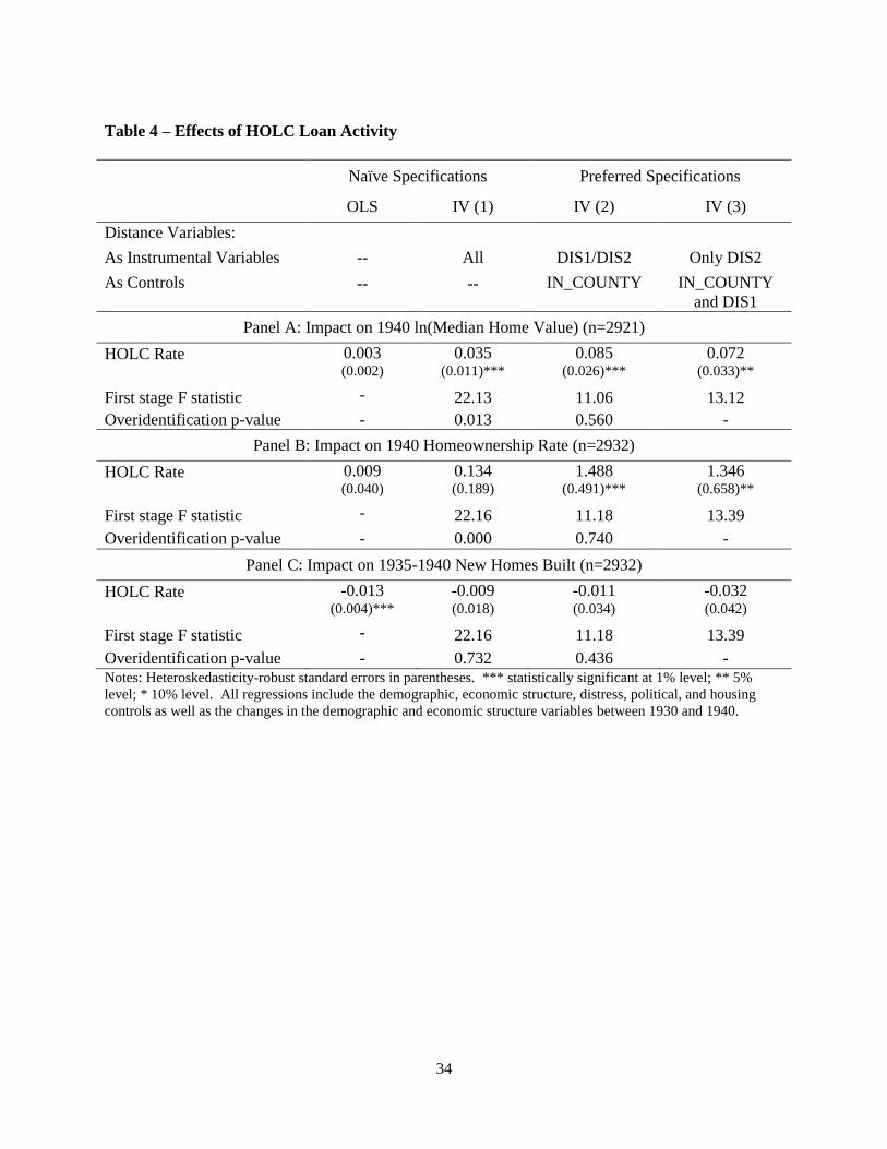
34

Table 4 – Effects of HOLC Loan Activity

Naïve Specifications Preferred Specifications

OLS IV (1) IV (2) IV (3)

Distance Variables:

As Instrumental Variables -- All DIS1/DIS2 Only DIS2

As Controls -- -- IN_COUNTY IN_COUNTY

and DIS1

Panel A: Impact on 1940 ln(Median Home Value) (n=2921)

HOLC Rate 0.003 (0.002)

0.035 (0.011)***

0.085 (0.026)***

0.072 (0.033)**

First stage F statistic - 22.13 11.06 13.12

Overidentification p-value - 0.013 0.560 -

Panel B: Impact on 1940 Homeownership Rate (n=2932)

HOLC Rate 0.009 (0.040)

0.134 (0.189)

1.488 (0.491)***

1.346 (0.658)**

First stage F statistic - 22.16 11.18 13.39

Overidentification p-value - 0.000 0.740 -

Panel C: Impact on 1935-1940 New Homes Built (n=2932)

HOLC Rate -0.013 (0.004)***

-0.009 (0.018)

-0.011 (0.034)

-0.032 (0.042)

First stage F statistic - 22.16 11.18 13.39

Overidentification p-value - 0.732 0.436 - Notes: Heteroskedasticity-robust standard errors in parentheses. *** statistically significant at 1% level; ** 5%

level; * 10% level. All regressions include the demographic, economic structure, distress, political, and housing

controls as well as the changes in the demographic and economic structure variables between 1930 and 1940.

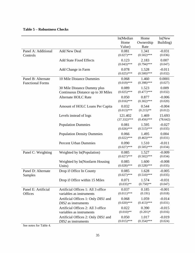
35

Table 5 – Robustness Checks

ln(Median

Home

Value)

Home

Ownership

Rate

ln(New

Building)

Panel A: Additional

Controls

Add New Deal 0.081 (0.027)***

1.341 (0.502)***

-0.031 (0.036)

Add State Fixed Effects 0.123 (0.043)***

2.183 (0.794)***

0.007 (0.047)

Add Change in Farm 0.078 (0.025)***

1.528 (0.500)***

-0.011 (0.032)

Panel B: Alternate

Functional Forms

10 Mile Distance Dummies 0.068 (0.019)***

1.460 (0.398)***

0.0001 (0.027)

30 Mile Distance Dummy plus

Continuous Distance up to 30 Miles

0.089 (0.025)***

1.523 (0.477)***

0.009 (0.032)

Alternate HOLC Rate 0.050 (0.016)***

0.877 (0.302)***

-0.006 (0.020)

Amount of HOLC Loans Per Capita 0.032 (0.013)***

0.544 (0.215)**

-0.004 (0.012)

Levels instead of logs 121.402 (37.332)***

1.469 (0.456)***

15.693 (78.642)

Population Dummies 0.081 (0.026)***

1.595 (0.515)***

-0.027 (0.035)

Population Density Dummies 0.066 (0.022)***

1.495 (0.463)***

0.004 (0.031)

Percent Urban Dummies 0.090 (0.027)***

1.510 (0.505)***

-0.011 (0.034)

Panel C: Weighting Weighted by ln(Population) 0.085 (0.027)***

1.527 (0.502)***

-0.009 (0.034)

Weighted by ln(Nonfarm Housing

Units)

0.085 (0.028)***

1.600 (0.528)***

-0.008 (0.035)

Panel D: Alternate

Samples

Drop if Office In County 0.085 (0.027)***

1.628 (0.510)***

-0.005 (0.035)

Drop if Office within 15 Miles 0.071 (0.035)**

1.574 (0.750)**

-0.031 (0.047)

Panel E: Artificial

Offices

Artificial Offices 1: All 3 office

variables as instruments

0.037 (0.011)***

0.185 (0.191)

-0.001 (0.018)

Artificial Offices 1: Only DIS1 and

DIS2 as instruments

0.068 (0.020)***

1.059 (0.413)***

-0.014 (0.031)

Artificial Offices 2: All 3 office

variables as instruments

0.022 (0.010)**

0.390 (0.201)*

-0.015 (0.016)

Artificial Offices 2: Only DIS1 and

DIS2 as instruments

0.050 (0.015)***

1.017 (0.354)***

-0.019 (0.024)

See notes for Table 4.

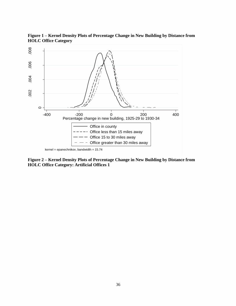
36

Figure 1 – Kernel Density Plots of Percentage Change in New Building by Distance from

HOLC Office Category 0

.00

2.0

04

.00

6.0

08

Den

sity

-400 -200 0 200 400Percentage change in new building, 1925-29 to 1930-34

Office in county

Office less than 15 miles away

Office 15 to 30 miles away

Office greater than 30 miles away

kernel = epanechnikov, bandwidth = 15.74

Figure 2 – Kernel Density Plots of Percentage Change in New Building by Distance from

HOLC Office Category: Artificial Offices 1

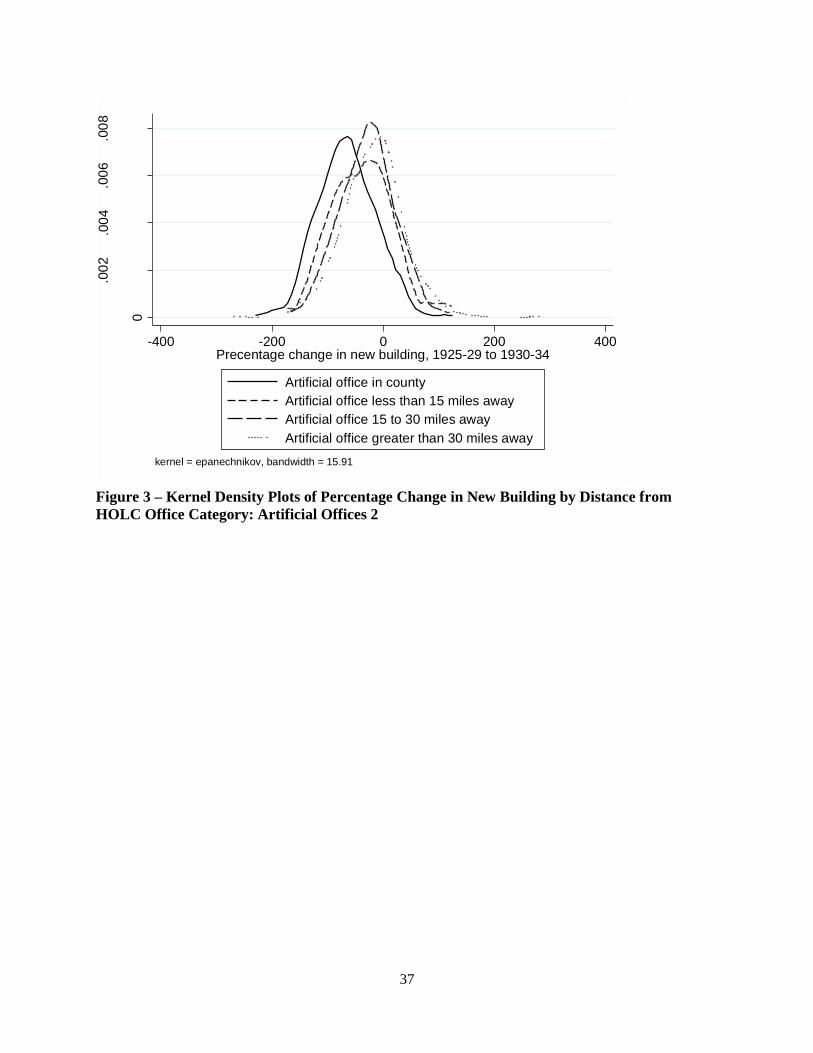
37

0

.00

2.0

04

.00

6.0

08

Den

sity

-400 -200 0 200 400Precentage change in new building, 1925-29 to 1930-34

Artificial office in county

Artificial office less than 15 miles away

Artificial office 15 to 30 miles away

Artificial office greater than 30 miles away

kernel = epanechnikov, bandwidth = 15.91

Figure 3 – Kernel Density Plots of Percentage Change in New Building by Distance from

HOLC Office Category: Artificial Offices 2

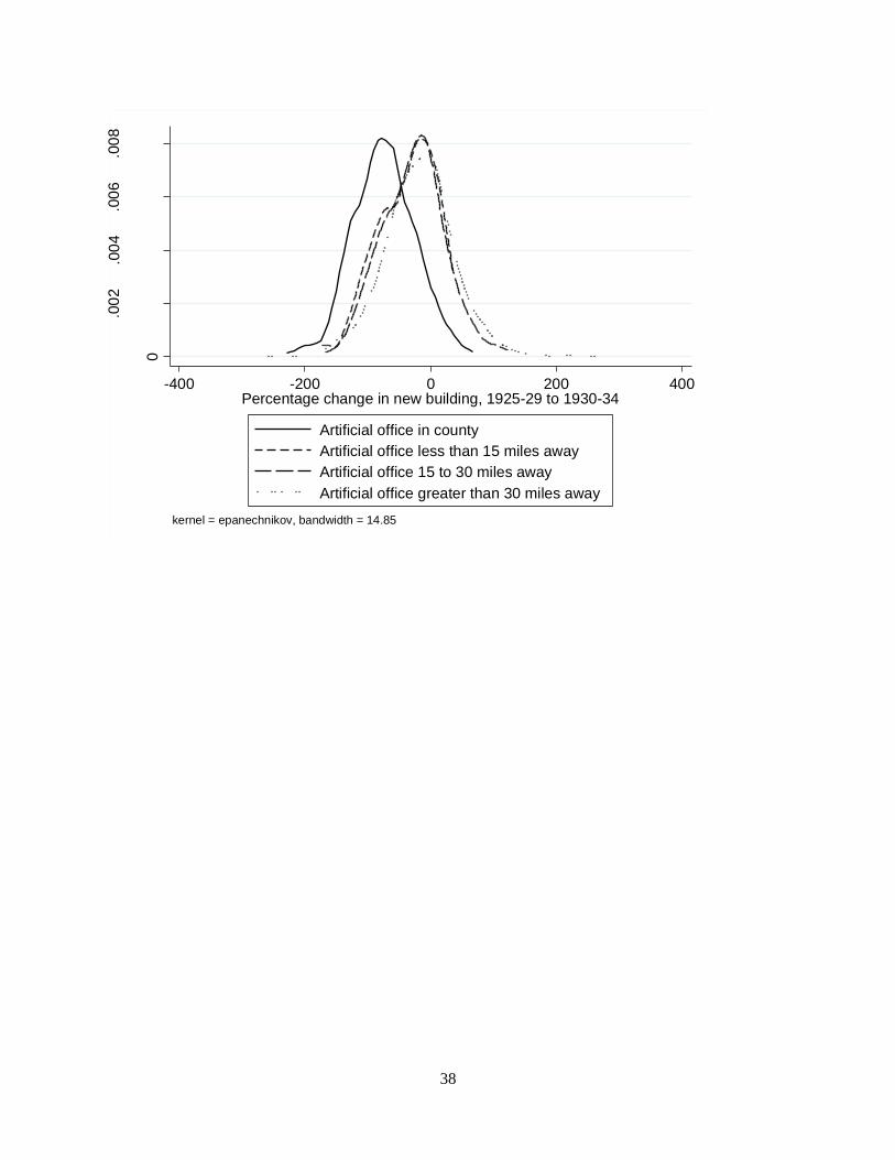
38

0

.00

2.0

04

.00

6.0

08

Den

sity

-400 -200 0 200 400Percentage change in new building, 1925-29 to 1930-34

Artificial office in county

Artificial office less than 15 miles away

Artificial office 15 to 30 miles away

Artificial office greater than 30 miles away

kernel = epanechnikov, bandwidth = 14.85