NBER WORKING PAPER SERIES

RENT RIGIDITY, ASYMMETRIC INFORMATION, AND VOLATILITY BOUNDSIN LABOR MARKETS

Bjoern BruegemannGiuseppe Moscarini

Working Paper 13030http://www.nber.org/papers/w13030

NATIONAL BUREAU OF ECONOMIC RESEARCH1050 Massachusetts Avenue

Cambridge, MA 02138April 2007

We thank seminar participants at the 2005 NBER Summer Institute, University of Connecticut, Yale,Hunter College, Tinbergen Institute, MIT, LABORatorio R.R., Harvard, Penn, 2006 SED, NYU andGeorgetown for comments. We gratefully acknowledge insightful conversations with Dino Gerardi.The views expressed herein are those of the author(s) and do not necessarily reflect the views of theNational Bureau of Economic Research.

© 2007 by Bjoern Bruegemann and Giuseppe Moscarini. All rights reserved. Short sections of text,not to exceed two paragraphs, may be quoted without explicit permission provided that full credit,including © notice, is given to the source.

Rent Rigidity, Asymmetric Information, and Volatility Bounds in Labor MarketsBjoern Bruegemann and Giuseppe MoscariniNBER Working Paper No. 13030April 2007JEL No. E24,E32

ABSTRACT

Recent findings have revived interest in the link between real wage rigidity and employment fluctuations,in the context of frictional labor markets. The standard search and matching model fails to generatesubstantial labor market fluctuations if wages are set by Nash bargaining, while it can generate fluctuationsin excess of what is observed if wages are completely rigid. This suggests that less severe rigiditymay suffice. We study a weaker notion of real rigidity, which arises only in frictional labor markets,where the wage is the sum of the worker's opportunity cost (the value of unemployment) and a rent.With wage rigidity this sum is acyclical; we consider rent rigidity, where only the rent is acyclical.We offer two contributions. First, we derive upper bounds on labor market volatility that apply if themodel of wage determination generates weakly procyclical worker rents, and that are attained by rentrigidity. Quantitatively, the bounds are tight: rent rigidity generates no more than a third of observedvolatility, an outcome that is closer to Nash bargaining than to wage rigidity. Second, we show thatthe bounds apply to a sequence of famous solutions to the bargaining problem under asymmetricinformation: at best they generate rigid rents but not rigid wages.

Bjoern BruegemannYale UniversityDepartment of EconomicsPO Box 208268New Haven, CT 06520-8268bjoern.bruegemann@yale.edu

Giuseppe MoscariniYale UniversityDepartment of EconomicsPO Box 208268New Haven, CT 06520-8268and NBERgiuseppe.moscarini@yale.edu

1 Introduction

The role of real wage rigidity in shaping employment fluctuations is a perennial subject of

macroeconomics. Interest in this subject has recently been revived by the finding that a

conventional calibration of the baseline textbook search and matching model driven by labor

productivity shocks of plausible magnitude and persistence grossly fails to account for the

observed volatility of unemployment and vacancies (Shimer, 2005; Hall, 2005; Costain and

Reiter, 2005). If the standard assumption of Nash-bargained wages is replaced by a rigid

wage, however, then the model is capable of generating fluctuations in excess of what is

observed (Hall, 2005). Thus in principle other models of wage determination may be able

to match observed volatility by generating wages which are not completely yet sufficiently

rigid. Specifically, Shimer (2005) asks whether bargaining under asymmetric information may

enhance amplification. What characteristics must a model of wage determination have in

order to match observed volatility?

In this paper we study a notion of rigidity weaker than wage rigidity. It arises naturally in

frictional labor markets, where the compensation of the worker is the sum of his opportunity

cost (the value of unemployed job search), and a quasi-rent that accrues when he finds a job.

With wage rigidity as in Hall (2005) overall compensation is acyclical. Because the value of

unemployment is higher in booms, when jobs are much easier to find, the worker’s quasi-rent

must be countercyclical to keep wages constant. We consider rent rigidity, where only the rent

component is acyclical, and ask the following question: must a model of wage determination

generate countercyclical rents to match observed volatility, or is rent rigidity sufficient?

Our answer is clear-cut: rent rigidity alone does not come close to matching observed

volatility. Second, we show that many famous and quite different solutions to the wage-

setting problem feature at best rent rigidity, but never wage rigidity. We put special but not

exclusive emphasis on environments with asymmetric information, thereby shedding light on

the question raised by Shimer. These are our two main contributions. We now provide some

details.

To show that rent rigidity alone can produce only very limited amplification, we derive

two upper bounds on labor market volatility, which apply if the model of wage determination

generates weakly procyclical worker rents, and are attained if rents are rigid. The first, weak

1

bound applies under mild regularity conditions on the model of wage determination, while

the second, strong bound applies under slightly more demanding conditions. The latter has

the advantage that only information from Shimer’s (2005) calibration is needed to conclude

that it is quantitatively tight : it allows for at most a third of observed volatility. The

same conclusion obtains for the weak bound if one additional element is added to Shimer’s

calibration: empirical information on the average cost of hiring a worker. Thus, unlike wage

rigidity, rent rigidity alone does not enable the model to generate labor market fluctuations

as large as in the data.

The mechanics behind the volatility bounds are as follows. Firms must be compensated

for the initial expense of hiring a worker by receiving quasi-rents over the life of the match.

Assume that worker rents are acyclical, the best case scenario for amplification if they cannot

be countercyclical. There are two possibilities, depending on the size of hiring costs.

First, suppose the average cost of filling a vacancy is small relative to overall gains from

trade in the labor market. In this case only small rents go to firms in compensation for hiring

costs, and worker rents must be large. In other words, finding a job yields unemployed workers

a large capital gain, both in booms and recessions as worker rents are acyclical. Now consider

an increase in the job finding rate. Since worker rents are large and constant, this has a large

positive effect on the opportunity cost of the worker: although the capital gain from finding a

job does not increase, it is large and more likely to accrue to the worker. Added to the constant

rents from employment, this larger value of unemployment translates one to one into a strong

increase in wages. Thus if an increase in productivity raises the job finding rate, then this

feedback effect through wages counteracts the increase in profits and thereby mutes vacancy

creation. Notice that this mechanism is similar to the reason why Nash bargaining generates

little amplification, with one important difference: with Nash bargaining the feedback effect

is driven both by an increase in worker rents and by an increase in the job finding rate. Rigid

rents preserve only the latter effect, but this is strong enough to severely curtail amplification.

The weak bound is solely based on this mechanism, which has bite only if hiring cost are

small. Evidence on hiring costs suggest that they are indeed small relative to overall gains

from trade, allowing us to conclude that the weak bound is quantitatively tight.

The strong bound requires no calibration of hiring costs, because it takes into account a

second effect which curtails amplification if hiring costs are large relative to overall gains from

2

trade in the labor market. In this case firms must receive large quasi-rents as compensation

for the initial hiring expense. Hence worker rents are small. While this weakens the feedback

effect, it introduces a second effect. The matching technology is such that a vacancy is less

likely to result in a match if the ratio of vacancies to unemployment in the economy is large, a

congestion effect. As a consequence, an increase in the vacancy-unemployment ratio induces

a proportional increase in the cost of filling a vacancy. If hiring costs are large on average,

this increase is large in absolute value. More importantly, if the increase in the vacancy-

unemployment ratio is caused by an increase in productivity, then the increase in hiring costs

is large relative to the original increase in productivity, once again muting vacancy creation.

To summarize our first contribution, rent rigidity is quantitatively much closer to Nash

bargaining than it is to wage rigidity. Thus merely switching to a different model of wage

determination does not allow the search and matching model to match observed volatility,

unless the model of wage determination is capable of generating countercyclical worker rents.

Our second contribution is to show that rent rigidity, thus our volatility bounds, apply to an

interesting class of models of wage determination. We focus on environments with asymmetric

information, thereby shedding light on Shimer’s question whether this can amplify the response

of the model to productivity shocks. We assume that, upon being matched, the firm privately

draws a match-specific productivity component and the worker a match-specific amenity value

of the job. The distributions are fixed and independent of (publicly observed) aggregate labor

productivity, and satisfy standard regularity conditions, but are otherwise unrestricted. In this

environment, we study in detail three classical wage determination models. In the monopoly

(or monopsony) solution, where either the firm or the worker makes a take-it-or-leave-it wage

proposal to the other privately informed party, it follows naturally that worker rents cannot

be countercyclical. If the firm is making the offer, it becomes more eager to trade in a boom,

and as a consequence it will concede more informational rents to the worker. If the worker is

making the offer, then in a boom once again firms are more eager to trade, thus the worker is

in a better position to extract rents through more aggressive wage requests. In both cases the

most that can be hoped for is no increase in worker rents in a boom. This basic intuition carries

over when we relax the commitment assumptions associated with take-it-or-leave-it offers, and

study strategic bargaining, both repeated one-sided offers (Coase conjecture) and alternating

offers. Finally, in an environment with bilateral asymmetric information, we consider the

3

constrained efficient allocation, obtained with the help of a mediator (e.g. an arbitrator in

wage contracting), as in Myerson and Satterthwaite (1983). Again we show that rent rigidity

is the most that can be obtained, for a similar reason: in a boom the mediator desires to induce

more trade, and in order to do so he has to increase informational rents going to workers.

To summarize our second contribution, at the very least asymmetric information intro-

duces, through the distribution of types, many additional degrees of freedom that can be

exploited to generate wage rigidity. In the models we study, however, these degrees of free-

dom are not enough to match observed labor market volatility.

Others have taken up Shimer’s question and investigated whether asymmetric information

enables the search and matching model to produce larger labor market fluctuations. Guerrieri

(2006) studies competitive search equilibrium, whereas we analyze bargaining games with

random matching, making the two analyses complementary. The approaches are different,

however. She simulates the model for some specific distributions of types. We derive labor

market volatility bounds that apply for any distribution of types. In fact, one can show that

our bounds also apply to her model. Her results are consistent with ours: she finds very little

amplification. Kennan (2006) and Menzio (2005b) take a different route, relying on exogenous

fluctuations in the shape of the distribution of types as the key driving force of labor market

fluctuations. In contrast, Guerrieri’s and this paper keep the extent of asymmetric information

itself acyclical, examining how the presence of asymmetric information amplifies the response

of the model to a productivity shock.

In Section 2 we introduce the economy. The labor market volatility bounds are derived

in Section 3. In Section 4 we verify these bounds for the models of wage bargaining under

asymmetric information. For simplicity, the analysis in Sections 2–4 restricts attention to

permanent labor productivity shocks. A fortiori, our results also apply to transitory shocks,

which generate a weaker response of the labor market. For completeness, Section 5 formally

derives the bounds for the case of transitory shocks, and provides an illustration using the

monopoly model. Section 6 concludes.

4

2 The Economy

We consider the baseline search-and-matching model employed by Shimer (2005). We extend

it to allow for bilateral asymmetric information about match-specific values: the worker may

have private information about how much he likes the job, and the firm may have private

information about productivity.

2.1 Preferences and Technology

The economy is populated by a measure 1 of workers and a much larger measure of firms. All

agents are infinitely-lived, risk neutral and share the discount rate r > 0. Workers can either be

employed or unemployed. An unemployed worker receives flow utility b and searches for a job.

Employed workers receive endogenously determined wage payments from their employers and

cannot search for other jobs. Firms can search for a worker by maintaining an open vacancy

at flow cost c. Free entry implies that the value of an open vacancy is zero. Unemployed

workers u and vacancies v are matched at rate m(u, v) where m is a constant returns to scale

matching function. Let θ ≡ vu

denote the vacancy-unemployment ratio. Then vacancies are

matched at rate m (1/θ, 1) ≡ q(θ) and workers are matched at rate m(1, θ) = θq(θ).

Upon being matched, the worker draws a match specific amenity value z from the distrib-

ution FZ and the firm draws a match specific productivity component y from the distribution

FY . The draws are once and for all until the match dissolves. Without loss in generality, the

two distributions have mean zero. Output of the match is given by p + y, so p is ex ante

average labor productivity. However, in general, not all matches are formed and p will not

equal labor productivity averaged across existing matches. We will refer to p as the aggregate

component of labor productivity. The amenity value z adds to the wage to determine the

flow value of employment for the worker. This value z may be private information of the

worker, and the idiosyncratic productivity component y may be private information of the

firm. Matches are destroyed exogenously at rate δ.

We want to study the magnitude of the response of the labor market to aggregate labor

productivity shocks. One way to proceed would be to specify a stochastic process for labor

productivity and evaluate the labor market volatility it induces. But to obtain upper bounds

on labor market volatility we can simply examine the response of the model to a permanent

5

unanticipated productivity shock. This response provides an upper bound to the volatility

induced by a stochastic process with transitory shocks for an intuitive reason: a given increase

in productivity increases incentives to create jobs more the longer it is expected to last.1 Of

course, this simpler approach introduces some slack and it may be possible to obtain tighter

bounds which explicitly account for the degree of persistence of productivity shocks. However,

due to the strong persistence of labor productivity in US data, the gain from such a tighter

bound would be quantitatively small. Thus the analysis in Sections 2–4 analyzes the case

of permanent productivity shocks, as the the cost of doing so is small relative to the gains

in terms of both simplicity and transparency of the analysis. In Section 5 we generalize the

analysis to the case of transitory shocks.

2.2 Wage Determination

Due to search frictions, a match generates quasi-rents. Thus we need to make assumptions

regarding how these rents are split between the worker and the firm. In other words, we need

a model of wage determination: a mapping of the relevant variables that describe the environ-

ment of the match into a decision whether to trade and how to split the quasi-rents associated

with the match. We work with a general definition of a model of wage determination, because

our objective is to obtain volatility bounds that apply to entire classes of models of wage

determination.

Here the assumption that productivity shocks are unanticipated and permanent keeps

matters simple: the environment of the match is characterized by only two aggregate variables.

The first is productivity p, which is expected to be constant over the life of the match. The

second variable is the endogenous opportunity cost of the worker, which is given by the

utility associated with unemployment U . It will be convenient to let n = rU represent

the opportunity cost of the worker in flow terms. This opportunity cost is a jump variable

1An extreme example may help in building intuition. Suppose matches last for several years on average.

Moreover, suppose that the economy switches between boom and recession every week. Clearly matches

created in booms and recessions are essentially the same, and the additional incentives to create matches in

booms are minimal relative to the case in which the economy switches from boom to recession only every few

years. See Section 5 as well as Mortensen and Nagypal (2005) and Hornstein, Krusell, and Violante (2005)

for a more formal development of this point.

6

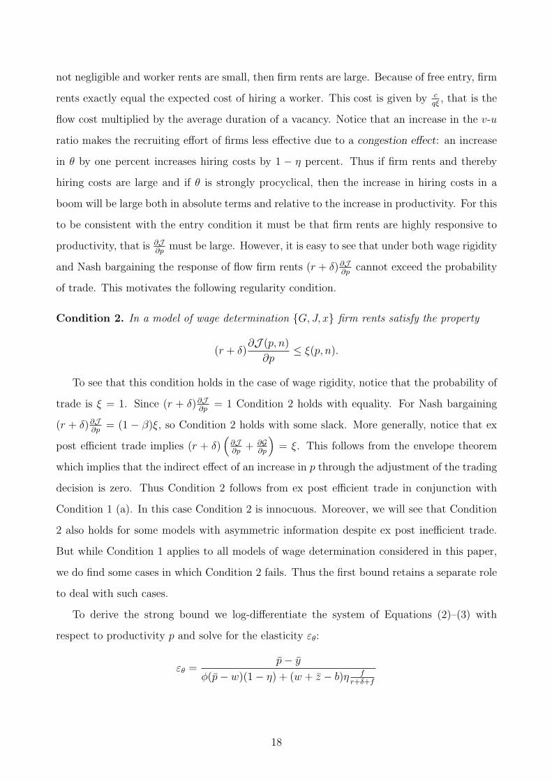
Figure 1: Model of Wage Determination

n w(p, n, y, z) + z

(r + δ)J(p, n, y, z)

(r + δ)G(p, n, y, z)

and constant along the equilibrium path of the economy following a productivity shock, a

convenient feature of the standard search and matching model.

For each pair of match-specific values y and z, a model of wage determination maps the

two variables p and n into a trade decision and a split of quasi-rents. It is important to

emphasize that the timing of wage payments over the life of a match is of no importance for

labor market fluctuations. Only the present value of rents going to the worker and the firm

matter. Thus we formulate a model of wage determination directly in terms of the present

values of rents.

Let G(y, z, p, n) denote the present value of rents going to the worker, J(y, z, p, n) denote

the present value of rents going to the firm, and x(y, z, p, n) be the probability that a match

is formed conditional on the realizations y and z.

Definition 1. A model of wage determination is a triple of functions {G, J, x} mapping R4

into R2+ × [0, 1] and satisfying

(r + δ) [G(y, z, p, n) + J(y, z, p, n)] = x(y, z, p, n)(y + z + p − n).

In terms of standard notation, the overall payoff of the employed worker is W = G + U ,

so G = W − U is the familiar capital gain an unemployed worker receives from being hired.

Although the timing of wage payments over the life of the match is not important, in order

to provide a link with wages, one can define the annuity value of the present value of wages

w(p, n, y, z) = (r + δ)G(y, z, p, n) + n − z, which would be the level of the wage if payments

were constant over the life of the match. Figure 1 illustrates the concept of a model of

wage determination. The entire bar represents the value of the match in flow terms, namely

7

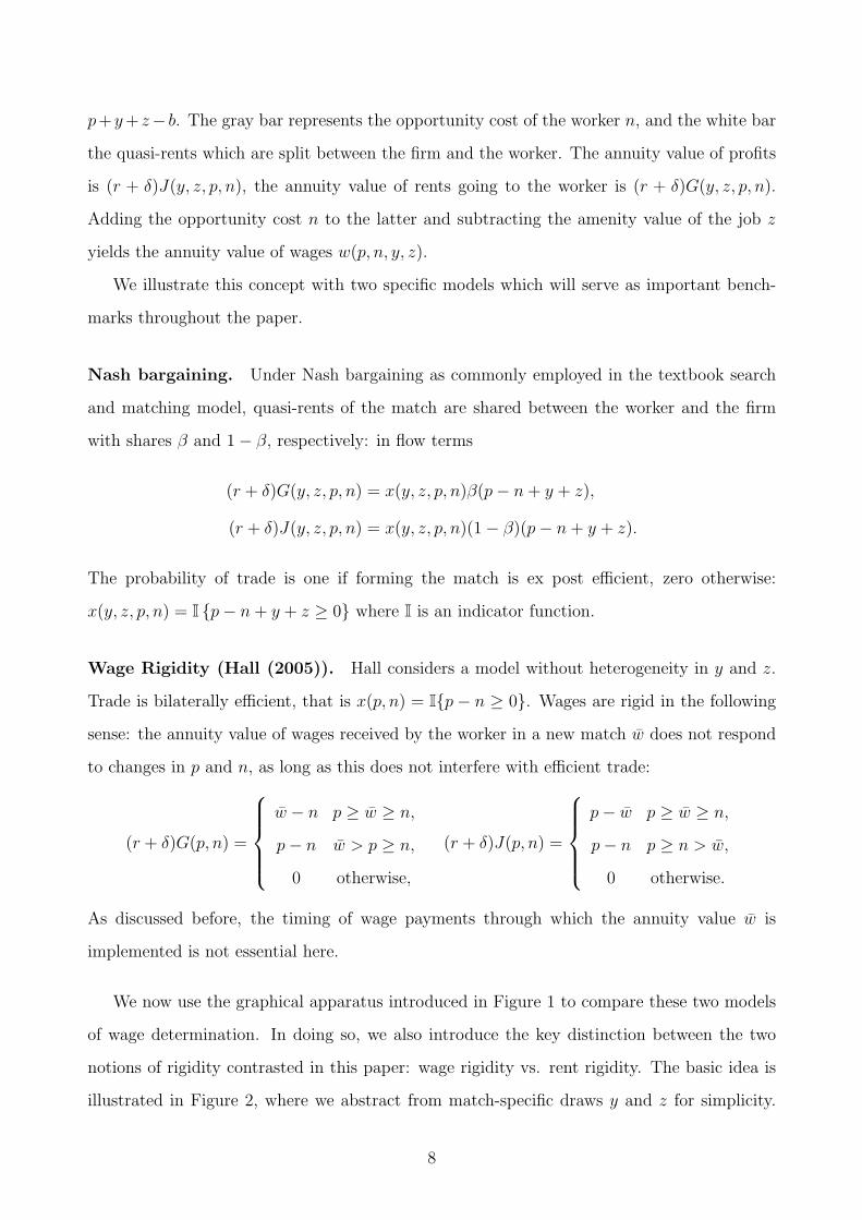
p+y + z− b. The gray bar represents the opportunity cost of the worker n, and the white bar

the quasi-rents which are split between the firm and the worker. The annuity value of profits

is (r + δ)J(y, z, p, n), the annuity value of rents going to the worker is (r + δ)G(y, z, p, n).

Adding the opportunity cost n to the latter and subtracting the amenity value of the job z

yields the annuity value of wages w(p, n, y, z).

We illustrate this concept with two specific models which will serve as important bench-

marks throughout the paper.

Nash bargaining. Under Nash bargaining as commonly employed in the textbook search

and matching model, quasi-rents of the match are shared between the worker and the firm

with shares β and 1 − β, respectively: in flow terms

(r + δ)G(y, z, p, n) = x(y, z, p, n)β(p − n + y + z),

(r + δ)J(y, z, p, n) = x(y, z, p, n)(1 − β)(p − n + y + z).

The probability of trade is one if forming the match is ex post efficient, zero otherwise:

x(y, z, p, n) = I {p − n + y + z ≥ 0} where I is an indicator function.

Wage Rigidity (Hall (2005)). Hall considers a model without heterogeneity in y and z.

Trade is bilaterally efficient, that is x(p, n) = I{p − n ≥ 0}. Wages are rigid in the following

sense: the annuity value of wages received by the worker in a new match w does not respond

to changes in p and n, as long as this does not interfere with efficient trade:

(r + δ)G(p, n) =

w − n p ≥ w ≥ n,

p − n w > p ≥ n,

0 otherwise,

(r + δ)J(p, n) =

p − w p ≥ w ≥ n,

p − n p ≥ n > w,

0 otherwise.

As discussed before, the timing of wage payments through which the annuity value w is

implemented is not essential here.

We now use the graphical apparatus introduced in Figure 1 to compare these two models

of wage determination. In doing so, we also introduce the key distinction between the two

notions of rigidity contrasted in this paper: wage rigidity vs. rent rigidity. The basic idea is

illustrated in Figure 2, where we abstract from match-specific draws y and z for simplicity.

8

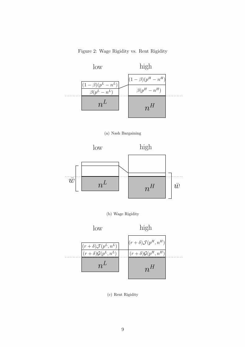
Figure 2: Wage Rigidity vs. Rent Rigidity

nL

(1 − β)(pL − nL)

β(pL − nL)

nH

(1 − β)(pH − nH)

β(pH − nH)

low high

(a) Nash Bargaining

nLwnH w

low high

(b) Wage Rigidity

nL

(r + δ)J (pL, nL)

(r + δ)G(pL, nL)

nH

(r + δ)J (pH , nH)

(r + δ)G(pH , nH)

low high

(c) Rent Rigidity

9

Each panel encompasses two replicas of Figure 1, one for a low aggregate state pL and one for

a high aggregate state pH > pL.

Panel (a) displays the case of Nash Bargaining. The quasi-rent is split with fixed shares

β and (1 − β). As the overall quasi-rent is procyclical, it follows that the rent going to the

worker is also procyclical.2

Panel (b) shows the case of wage rigidity. Even with rigid wages the opportunity cost of

workers are procyclical in the stochastic equilibrium of the economy.3 As shown in the figure,

this implies that rents must be countercyclical.

Panel (c) illustrates the contrast with the notion of rent rigidity. Here the rent going to the

worker does not increase in a boom, but the annuity value of wages w(p, n) increases because

the opportunity cost of the worker n does. In this sense, rent rigidity is weaker than wage

rigidity.

It is instructive to relate rent rigidity to Nash bargaining with an ad hoc countercyclical

bargaining share β(p). Shimer (2005) shows in a reduced form experiment that making the

bargaining share somewhat countercyclical helps in generating more volatile unemployment

and vacancies. We emphasize that a countercyclical bargaining share per se does not imply

countercyclical rents. It is clear from Figure 2 (c) that if the bargaining share is only slightly

countercyclical, then rents remain procyclical. As one continues to make the bargaining share

more countercyclical, eventually the qualitative threshold will be crossed at which rents also

become countercyclical. One way of putting the question we will answer in the next section

is then as follows: do we need to cross this threshold in order to generate the observed extent

of volatility?

2.3 Equilibrium Conditions

Having defined models of wage determination we can now write down the equilibrium condi-

tions of the model. Before doing so, it is useful to make precise how we will evaluate the extent

of labor market volatility generated by the model. We follow the literature and focus on the

2Procyclicality of the overall quasi-rent is an equilibrium implication of the standard search and matching

model with Nash bargaining, which we discuss in detail in Section 3.3As we will show in Section 3, in a boom, even though unemployed workers do not get a higher wage should

they find a job, they are more likely to find a job, so the value of unemployment increases.

10

vacancy-unemployment ratio θ = vu

rather than unemployment and vacancies separately. In

US data, detrended vacancies and unemployment are strongly negatively correlated, so their

ratio is especially volatile. Thus the volatility of the v-u ratio presents a convenient way of

capturing the challenge facing the model in a single statistic.4

The model has two endogenous variables: the v-u ratio θ and the opportunity cost of the

worker n. Both immediately jump to their new steady state values in response to a permanent

productivity shock.5 Thus one can compute the elasticity εθ of the v-u ratio with respect to

a productivity shock by differentiating the steady state equations of the model.

Given a model of wage determination, we can compute the ex ante (before matching)

averages of rents and the probability of trade

G(p, n) ≡

∫∫G(y, z, p, n)dFY (y)dFZ(z),

J (p, n) ≡

∫∫J(y, z, p, n)dFY (y)dFZ(z), (1)

ξ(p, n) ≡

∫∫x(y, z, p, n)dFY (y)dFZ(z).

With this notation we study two steady state conditions in (θ, n).6 First, the free entry

condition, equating the flow cost of posting a vacancy c to the expected capital gain, which is

the rate q(θ) at which open vacancies meet a worker, times the expected value J (p, n) to the

firm of meeting a worker, taking into account that the match may potentially fail to form:

c = q(θ)J (p, n). (2)

Second, the equation determining the flow value of unemployment as the flow value of leisure

b plus the expected capital gain, the rate θq(θ) at which unemployed workers contact open

vacancies times the expected return G(p, n) from the contact, again taking into account that

the match may potentially fail to form:

n = b + θq(θ)G(p, n). (3)

4Moreover, as discussed by Shimer (2005) the model already does reasonably well at capturing comove-

ment and relative volatility of unemployment and vacancies. In this sense there is little need to examine

unemployment and vacancies separately, and it is sufficient to focus on the volatility of the v-u ratio.5Pissarides (2000), pp. 26-33.6Once θ = v

uhas been computed from these conditions, steady state levels of unemployment u and then

vacancies v = θu are computed using the Beveridge curve u = δδ+θq(θ) . Since we focus on the v-u ratio we do

not make use of this relationship.

11

3 Labor Market Volatility Bounds

In this section we derive two bounds on labor market volatility and evaluate them quantita-

tively. These bounds apply to models of wage determination which generate weakly procycli-

cal, that is at best rigid but not countercyclical, worker rents.

So far we have not put any structure on the three functions that make up the model of

wage determination. We now introduce a set of regularity conditions. They are quite weak

and are satisfied by all models of wage determination considered in this paper, including Nash

bargaining and wage rigidity. This is important since we are interested in models of wage

determination which lie in some sense in between these two benchmark models.

Condition 1. The model of wage determination {G, J, x} satisfies three properties:

(a) The partial effect of aggregate labor productivity p on ex ante worker rents is non-

negative: for all p, n,∂G(p, n)

∂p≥ 0.

(b) The partial effect of the worker’s opportunity cost n on ex ante firm rents is non-positive:

for all p, n,∂J (p, n)

∂n≤ 0.

(c) The trade probability x(p, n, y, z) depends on p and n only through their difference p −

n, and is weakly increasing in both match-specific outcomes, the firm’s idiosyncratic

productivity component y and the worker’s amenity value for the job z.

Part (a) requires that holding worker opportunity cost n constant, an increase in labor

productivity will not reduce worker rents. Importantly, this does not imply procyclical worker

rents: under wage rigidity the partial effect of labor productivity is exactly zero; thus worker

rents are countercyclical as worker opportunity costs n increase in booms. Similarly, part (b)

does not imply that firm profits are countercyclical. Again wage rigidity represents the extreme

case in which the partial effect is zero; firm rents under wage rigidity are then procyclical as

the productivity component p is higher in booms.

Both Nash bargaining and wage rigidity feature ex post efficient trade, that is trade occurs

if and only if p−n+ y + z ≥ 0. Ex post efficiency immediately implies part (c). The converse

12

is not true, that is part (c) is weaker than ex post efficiency. We will see that part (c)

holds for all the models featuring ex post inefficient trade considered in Section 4. For an

interpretation of this property, first consider comparative statics with respect to p and n. If p

and n increase by the same amount, this shifts up the location of the bargaining problem to

a higher level of productivity and opportunity cost, but leaves the average gains from trade

p − n unchanged. Condition 1 (c) requires that such a shift leaves the probability of trade

unaffected. The second requirement of Condition 1 (c) specifies that matches are positively

selected. Let y(p, n) ≡ ξ(p, n)−1∫∫

x(p, n, y, z)ydFY (y)dFZ(z) be the average match specific

productivity component conditional on trade. Condition 1 (c) implies y(p, n) ≥ 0.7 Similarly,

it implies that the conditional mean amenity value z(p, n) is non-negative.

We now derive two bounds on labor market volatility, referred to as weak and strong,

respectively. The weak bound is less tight theoretically, and more empirical information must

be utilized in order to conclude that it is tight quantitatively. The second bound holds under

more stringent conditions on the model of wage determination.

3.1 Weak Labor Market Volatility Bound

The first bound applies to all models of wage determination that satisfy the following property

(along with regularity Condition 1).

Definition 2. (Increasing Worker Rents) In a model of wage determination {G, J, x},

worker rents are Increasing if, for all p, n,

∂G(p, n)

∂p≥ −

∂G(p, n)

∂n≥ 0.

Notice that this property is stronger than Condition 1 (a): the partial effect of aggregate

labor productivity p on worker rents is not only non-negative, but it is required to exceed in

absolute value the effect of the worker’s opportunity cost n on worker rents.

To explain the role of Increasing worker rents, it is useful to define the following property

of the equilibrium.

Definition 3. (Procyclical Worker Rents) Worker rents are Procyclical in equilibrium

7Recall that the unconditional mean of match specific productivity has been normalized to zero.

13

ifdG(p, n)

dp=

∂G(p, n)

∂p+

∂G(p, n)

∂n

dn

dp≥ 0.

As will emerge clearly from the derivation, the weak labor market volatility bound applies

whenever worker rents are Procyclical in equilibrium. Procyclicality, however, is a feature

of the equilibrium and not a condition that can be verified only examining the model of

wage determination. Increasing worker rents is a sufficient condition on the model of wage

determination which insures that worker rents are Procyclical in equilibrium.

We obtain the volatility bound for θ in three steps. First we show that if worker rents are

Procyclical and the elasticity εθ = d ln θ/d ln p has to be positive, then the opportunity cost

of the worker responds less than one for one to an increase in productivity, that is dndp

< 1.

Second we transform this inequality for dndp

into the desired upper bound on εθ, which applies

whenever worker rents are Procyclical. Finally we show that if worker rents are Increasing,

then they are Procyclical.

First, we show that εθ > 0 implies dndp

< 1. If the increase in the outside option of the

worker in a boom was so large as to overturn the increase in productivity, then firm rents

would shrink, which is inconsistent with more intensive hiring activity of firms. We refer to

∂J∂n

dndp

as the feedback effect, as it captures how an increase in profits that raises vacancies and

thereby the job finding rate feeds back negatively into profits through a higher opportunity

cost of workers. To see that firm profits must shrink, namely dJdp

≤ 0, if dndp

≥ 1, first suppose

that ∂J∂p

≤ 0. Then both the increase in productivity and — by virtue of part Condition 1

(b) — the increase in n reduce firm profits. If instead ∂J∂p

≥ 0 it follows from parts (a) and

(c) of Condition 1 that the sum of worker and firm rents must be increasing in p− n. In this

case dndp

≥ 1 implies that total rents fall, and Procyclical worker rents imply that once again

firm rents must decrease. Through the entry condition (2) lower firm rents in turn imply that

labor market tightness must fall, contradicting εθ > 0.

Second, from Equation (3), it is clear that an increase in worker rents raises the opportunity

cost n: a larger capital gain from finding a job increases the utility of unemployed workers.

Specifically, Procyclical worker rents and Equation (3) imply the following lower bound on

dndp

:dn

dp≥ ηεθθq

G

p. (4)

14

Here η ≡ 1 − dq

dθθq

denotes the elasticity of the matching function with respect to vacancies,

evaluated at the initial equilibrium. Similarly, θ, q, and G are the v-u ratio, the contact rate of

vacancies, and worker rents, all evaluated at the initial equilibrium. Inequality (4) holds as an

equality if worker rents are completely rigid. Notice that even in that case dndp

is positive: the

value of unemployment increases because it is easier to find a job. Moreover, a large elasticity

εθ implies that the job finding rate responds strongly to an increase in productivity, leading

to a larger value of dndp

. Combining (4) with dndp

< 1 from the first step implies an upper bound

on the elasticity εθ

εθ ≤1

η

1

θq

p

G. (5)

The interpretation of this upper bound is straightforward. If η is large, then the job finding

rate responds strongly to an increase in θ because vacancies are very productive in the creation

of matches. This is associated with a stronger feedback effect and leads to a tighter bound on

εθ. If the job-finding rate θq is larger, then a given percentage increase in θ translates into a

larger increase in the chances of finding a job, also tightening the bound. Finally, the bound

is tighter if the level of rents going to the worker is higher. If the capital gain of finding a job

is zero, then a higher job-finding rate does not translate into a higher value of unemployment

because there is nothing to be gained from finding a job.

To turn (5) into a bound that can be evaluated quantitatively we need to calibrate worker

rents G. For this purpose we introduce some additional notation. First the annuity value of

wages in the initial equilibrium is w ≡ (r + δ)ξ−1G + n − z (recall that the average amenity

value z must be deducted from the average flow utility of an employed worker in order to

obtain wages). Next define the job finding rate

f ≡ θqξ,

which is the product of the matching rate θq and the probability of match formation ξ. Finally

define observed average labor productivity, the average of p+y conditional on trade p ≡ p+ y.

Using this notation together with Equation (3) we can rewrite (5) as

εθ ≤p − y

w + z − b

1

η

r + δ + f

f.

At this point we use Condition 1 (c): the fact that matches that do form are positively selected

15

implies that y ≥ 0 and z ≥ 0. This yields

εθ ≤p

p − b

p − b

w − b

1

η

r + δ + f

f≡ εθ,WEAK .

The third and final step is to show that if worker rents are Increasing, then they are

Procyclical. Suppose not. This can only happen if dndp

> 1. Increasing worker rents in

conjunction with Condition 1 (c) imply ∂J∂p

+ ∂J∂n

≤ 0. Thus dndp

> 1 and Condition 1 (b)

imply that firm rents decrease in response to an increase in p. For firms to be willing to post

vacancies in the face of lower rents the v-u ratio must fall, that is equilibrium condition (2)

implies εθ ≤ 0. But with both worker rents and the job finding rate countercyclical it follows

from Equation (3) that the utility of unemployed workers must be lower, that is dndp

≤ 0, a

contradiction.

We have established the following:

Proposition 1. (Weak Volatility Bound) If the model of wage determination satisfies

Condition 1 and worker rents are Procyclical, then εθ ≤ εθ,WEAK. If worker rents are Increas-

ing, then they are Procyclical.

Our approach in Section 4 is to show that a given model of wage determination under

asymmetric information satisfies both Condition 1 and Increasing worker rents. Proposition 1

then allows us to conclude that this model of wage determination is subject to the weak labor

market volatility bound. Proposition 1 can also be applied in a different way: if a model of

wage determination satisfies Condition 1 but generates amplification in excess of the bound,

then it must produce countercyclical worker rents. That is, finding a job yields a larger gain

in a slump. We illustrate this application with the following model of wage determination.

Outside Option Principle. Hall and Milgrom (2007) consider the bargaining theory of

Binmore, Rubinstein, and Wolinsky (1986). According to this theory, the relevant threat

point of the worker is not unemployment but delay of bargaining, say a strike. Let bs be the

flow payoff of the worker during a strike, which could be different from the flow payoff during

unemployment b. The game has a unique subgame perfect equilibrium which yields a wage

w(p, n) = bs + 12(p − bs). This is similar in form to the Nash bargaining wage, but with the

strike value bs replacing the opportunity cost n. The model is given by x(p, n) = I{p−n ≥ 0}

16

and

(r + δ)G(p, n) =

12(p + bs) − n 1

2(p + bs) ≥ n,

0 otherwise,

(r + δ)J(p, n) =

12(p − bs) 1

2(p + bs) ≥ n,

p − n p ≥ n ≥ 12(p + bs),

0 otherwise.

Condition 1 is easily verified, but since ∂G∂p

+ ∂G∂n

= −12

worker rents are not Increasing.

Moreover, with an elasticity

εθ,HM =1

1 − η

p

p − bs

the model can generate a volatility exceeding the bound εθ,WEAK , by choosing bs sufficiently

close to p. However, Proposition 1 allows us to conclude that the only way this can occur is

if the model generates countercyclical worker rents in equilibrium. This is not obvious, as in

principle the model can generate procyclical worker rents if bs is sufficiently close to b.8

3.2 Strong Labor Market Volatility Bound

We now derive a second volatility bound which is stronger in that it uses more theory, is

qualitatively tighter. Moreover, less empirical information is required to conclude that it is

quantitatively tight.

As the starting point, notice that the derivation of the weak bound was based almost

entirely on the second equilibrium condition (3). The entry condition (2) was used only to a

limited extent, to show that a more than one for one response of opportunity costs dndp

≥ 1

is inconsistent with a positive elasticity εθ. In particular, the weak bound is based on the

feedback effect arising from condition (3). As we discussed this effect is strong if the annuity

value of wages and thus worker rents are large. As the annuity value of wages approaches b (or

equivalently worker rents approach zero) the feedback effect vanishes and the bound becomes

very loose, asymptoting to infinity.

We now show that if worker rents are small, then a second effect neglected by the weak

bound comes into play and limits amplification. The strong bound is obtained by fully ex-

ploiting the entry condition. The mechanics are as follows. If total rents from a match are

8One can check that worker rents are procyclical for b = bs under Shimer’s calibration.

17

not negligible and worker rents are small, then firm rents are large. Because of free entry, firm

rents exactly equal the expected cost of hiring a worker. This cost is given by cqξ

, that is the

flow cost multiplied by the average duration of a vacancy. Notice that an increase in the v-u

ratio makes the recruiting effort of firms less effective due to a congestion effect: an increase

in θ by one percent increases hiring costs by 1 − η percent. Thus if firm rents and thereby

hiring costs are large and if θ is strongly procyclical, then the increase in hiring costs in a

boom will be large both in absolute terms and relative to the increase in productivity. For this

to be consistent with the entry condition it must be that firm rents are highly responsive to

productivity, that is ∂J∂p

must be large. However, it is easy to see that under both wage rigidity

and Nash bargaining the response of flow firm rents (r + δ)∂J∂p

cannot exceed the probability

of trade. This motivates the following regularity condition.

Condition 2. In a model of wage determination {G, J, x} firm rents satisfy the property

(r + δ)∂J (p, n)

∂p≤ ξ(p, n).

To see that this condition holds in the case of wage rigidity, notice that the probability of

trade is ξ = 1. Since (r + δ)∂J∂p

= 1 Condition 2 holds with equality. For Nash bargaining

(r + δ)∂J∂p

= (1 − β)ξ, so Condition 2 holds with some slack. More generally, notice that ex

post efficient trade implies (r + δ)(

∂J∂p

+ ∂G∂p

)= ξ. This follows from the envelope theorem

which implies that the indirect effect of an increase in p through the adjustment of the trading

decision is zero. Thus Condition 2 follows from ex post efficient trade in conjunction with

Condition 1 (a). In this case Condition 2 is innocuous. Moreover, we will see that Condition

2 also holds for some models with asymmetric information despite ex post inefficient trade.

But while Condition 1 applies to all models of wage determination considered in this paper,

we do find some cases in which Condition 2 fails. Thus the first bound retains a separate role

to deal with such cases.

To derive the strong bound we log-differentiate the system of Equations (2)–(3) with

respect to productivity p and solve for the elasticity εθ:

εθ =p − y

φ(p − w)(1 − η) + (w + z − b)η f

r+δ+f

18

where the term

φ ≡ξ + f

∂G

∂p+ ∂G

∂ndndp

1− dndp

(r + δ)

(∂J∂p

+ ∂G∂p

−∂G

∂p+ ∂G

∂ndndp

1− dndp

) (6)

equals one if the equilibrium exhibits acyclical worker rents and if the trading decision is ex

post efficient. Thus deviations of φ from one capture departures from these two properties. We

first show that Increasing worker rents in conjunction with Condition 2 implies φ ≥ 1. First

recall from Proposition 1 that if worker rents are Increasing, then they are Procyclical. This

allows us to bound the numerator in Equation (6) from below by (r + δ)∂J∂p

. Moreover, this

also implies ∂G∂p

−∂G

∂p+ ∂G

∂ndndp

1− dndp

≤ 0. Together with Condition 2 this insures that the denominator

is bounded from above by ξ. Thus φ ≥ 1 as desired. When this is combined with positive

selection z ≥ 0 and y ≥ 0 from Condition 1 (c), then Equation (6) yields the strong volatility

bound

εθ ≤p

p − b

(p − w

p − b

11

1−η︸ ︷︷ ︸congestion

+w − b

p − b

11η

r+δ+f

f︸ ︷︷ ︸feedback

)−1

≡ εθ,STRONG. (7)

The first term p

p−bof the product in Equation (7) captures the percentage increase in the flow

gain from market activity p − b associated with a percentage increase in labor productivity

p. If b is close to p, then the flow gains from market activity are very elastic with respect

to productivity. Thus everything else equal a large b enables the model to generate large

fluctuations in the v-u ratio.

Next consider the second term, the harmonic weighted mean of the two terms 11−η

and

1η

r+δ+f

f. The latter is familiar from the first bound and captures the feedback effect. The

weight on this term in the mean is the fraction of the gains from market activity going to

the worker w−bp−b

: as was reflected in the first bound, the feedback effect puts a tighter limit

on amplification if the annuity value of wages is large. The first term of the weighted average

11−η

is new and captures the congestion effect. This effect is more severe if η is low, that is if

an increase in the v-u ratio has a strong negative effect on the rate at which vacancies contact

workers. The weight on this term is the fraction of the gains from market activity going to

firms. Recall that this fraction is large precisely when the level of hiring costs is large. A large

level of hiring costs combined with a low η means that the absolute increase in hiring costs in

a boom is large relative to the increase in productivity, putting a tight limit on amplification.

19

We have established the following:9

Proposition 2. (Strong Volatility Bound) If the model of wage determination satisfies

Conditions 1 and 2 and if worker rents are Increasing, then εθ ≤ εθ,STRONG.

We now show how the strong bound can be attained. This is of theoretical interest because

one would like to know whether the bound is tight for the class of models of wage determination

satisfying Conditions 1 and 2. It will also turn out to be of some interest quantitatively to

the extent that the bound allows for some amplification vis-a-vis Nash bargaining.

Complete Rent Rigidity. Consider the following mode of wage determination. Trade is

bilaterally efficient, that is x(p, n) = I{p−n ≥ 0}. The worker receives a fixed flow rent g > 0

which does not respond to changes in p and n, unless it would interfere with efficient trade:

(r + δ)G(p, n) =

g p ≥ n + g,

p − n n + g > p ≥ n,

0 otherwise,

(r + δ)J(p, n) =

p − n − g p ≥ n + g,

0 otherwise.

Notice that worker rents are acyclical by construction. Conditions 1 and 2 are easily verified.

It is straightforward to check that the elasticity of the v-u ratio generated by the model is

exactly εθ,STRONG, where the annuity value of wages is related to the rent parameter g through

the formula g = r+δr+δ+f

(w − b). This model is ad hoc in the same way as Hall’s rigid wage. In

analogy to Hall (2005), one may think of it as an alternative equilibrium selection of a double

auction, and interpret it as a norm or social consensus which applies to worker rents rather

than the level of wages. An alternative well-known model of wage determination that delivers

complete rent rigidity is the Shapiro and Stiglitz (1984) efficiency wage shirking model.10

9The weak bound applies not only if worker rents are Increasing, but also if they are just Procyclical. For

the strong bound we can obtain an analogous result, but it requires a stronger version of Condition 2. If

worker rents are Procyclical but not Increasing, then we cannot conclude that ∂G∂p

−∂G∂p

+ ∂G∂n

np

1− dndp

≤ 0. To insure

that φ ≥ 1 we need to strengthen (r+δ)∂J∂p

≤ ξ to (r+δ)(

∂J∂p

+ ∂G∂p

)≤ ξ. If the model of wage determination

satisfies this property along with Condition 1, then the strong bound applies if worker rents are Procyclical.10 According to Equation (5) in their paper, the worker receives a flow rent g = (r+δ+q)e

qwhere e is the

cost to the worker of providing effort, and q is the rate at which a shirking worker is caught. Thus rents are

completely rigid in response to a shock to aggregate labor productivity as long as both e and q do not vary

with productivity p.

20

An interesting question is whether the bound can be attained not only through complete

rent rigidity, but also by the models of wage determination under asymmetric information

considered in Section 4. There we provide an affirmative answer for the monopoly model.

The model of complete rent rigidity attains the strong bound. The difference between

the two bounds is that the first bound neglects the congestion effect. This implies that the

weak bound cannot be attained by any model of wage determination that generates a non-

zero congestion effect. The congestion effect is positive as long as ∂J∂p

is finite. With ex post

efficient trade this is always the case. Since the model of complete rent rigidity features ex

post efficient trade, it cannot attain the weak bound. Introducing ex post inefficient trade in

an ad hoc fashion into the model of complete rent rigidity would enable it to attain the weak

bound.11

3.3 Calibration

We now evaluate the two volatility bounds quantitatively and compare them to Nash bargain-

ing and wage rigidity. To make this comparison we need to compute the elasticities of the

v-u ratio associated with these models of wage determination. In analogy to the bounds we

express these elasticities in terms of the parameters η, p, b, r, δ, together with the equilibrium

job finding rate f and the equilibrium annuity value of wages w. The formulas are written to

facilitate comparison with the bounds:

εθ,NASH =p

p − b

(11

1−η

+w − b

p − b

11η

r+δ+f

f

)−1

, εθ,HALL =p

p − b

(p − w

p − b

11

1−η

)−1

,

for Nash bargaining and wage rigidity, respectively.12 Nash bargaining differs from the strong

bound through a higher weight on the term 11−η

, which stems from the procyclicality of rents.

Wage rigidity differs through a zero weight on 1η

r+δ+f

f, as it completely severs the feedback

effect. Our quantitative evaluation is based Shimer’s (2005) calibration, which is displayed

in Table 1. The model period is a quarter. The interest rate is chosen to match an annual

discount factor of 0.953. Shimer infers time series of quarterly separation and job finding

11Let ξ(p−n) = eζ(p−n) be the probability of trade. Set (r+δ)J(p, n) = ξ(p−n)(p−n)−g if ξ(p−n)(p−n) ≥ g,

setting it to zero otherwise. Then the weak bound is attained for ζ → ∞.12In the case of Nash bargaining the annuity value of wages is related to the bargaining parameter through

w = (r+δ)[(1−β)b+βp]+βfp

(r+δ)+βf. With wage rigidity the annuity value of wages is simply the rigid wage w = w.

21

Table 1

Parameter Value

r 0.012

δ 0.1

η 0.28

bp

0.4

f 1.35

β 0.72

rates from BLS data. He sets δ equal to the average separation rate of 0.1. The data on

the job finding rate together with data on the v-u ratio is used to estimate the matching

function elasticity, yielding η = 0.28. Given the value of the matching function elasticity,

Shimer chooses the Nash bargaining parameter β such that the Hosios (1990) condition is

satisfied, that is β = 1 − η = 0.72.13 It is more difficult to calibrate the value of non-market

activity b. If one is willing to assume that it stems solely from unemployment benefits one

can use replacement rates. Proceeding along these lines Shimer sets bp

= 0.4. We return to

the calibration of this parameter below.

Notice that the vacancy cost c does not appear in the table. It is pinned down by calibrating

the model to match the average job finding rate f = 1.35.

Shimer’s calibration provides all the information needed to evaluate the bounds except

for the annuity value of wages (normalized by productivity) wp. In his calibration of the

model with Nash bargaining Shimer does not need to directly calibrate the annuity value of

wages since it is pinned down by choosing the bargaining parameter β to satisfy the Hosios

condition. The implied value is wNB

p= 0.9826. When calibrating the model with a rigid wage,

Hall (2005) and Shimer (2004) must choose a level of the rigid wage and thus of the annuity

value of wages. They sidestep the issue of independently calibrating the wage by adopting

the level implied by the model with Nash bargaining under the Hosios condition. We could

proceed in the same way. It is desirable, however, to calibrate the wage level independently,

13Shimer assumes a Cobb-Douglas matching function, for which β = 1 − η implies social efficiency of the

equilibrium.

22

using data on hiring costs. To see how this works, notice that Equation (2) can be written as

c

qξ=

p − w

r + δ. (8)

The left hand side is the expected cost of hiring a worker, that is the flow cost c times the

expected duration of a vacancy 1qξ

. Over the life of the match the firm receives the flow p−w.

The present value of this flow must be such that the firm recoups the initial hiring costs. Both

Silva and Toledo (2007) as well as Hagedorn and Manovskii (2006) utilize evidence provided by

Barron, Berger, and Black (1997) which in turn is based on the 1982 Employment Opportunity

Project and the 1992 Small Business Administration survey. This evidence suggests that the

average labor cost of hiring a worker corresponds to between 3 and 4.5 percent of the quarterly

wage. This does not include costs such as advertisement, and citing further evidence Silva

and Toledo (2006) argue that total hiring costs could be as high as 14 percent of the quarterly

wage. This is close to the estimate of 13 percent provided by Abowd and Kramarz (2003)

for French data. For our purposes it suffices to identify a region in which hiring costs could

reasonably lie. Proceeding conservatively based on the evidence above we consider hiring costs

between 3 percent and 30 percent of quarterly wages. Using Equation (8) this yields a range[

wmin

p, wmax

p

]= [0.9675, 0.9967] for the wage w

p. Notice that the wage level wNB

pimplied by

the model with Nash bargaining under the Hosios condition is contained in this range and

corresponds to hiring costs of 16 percent of quarterly wages.

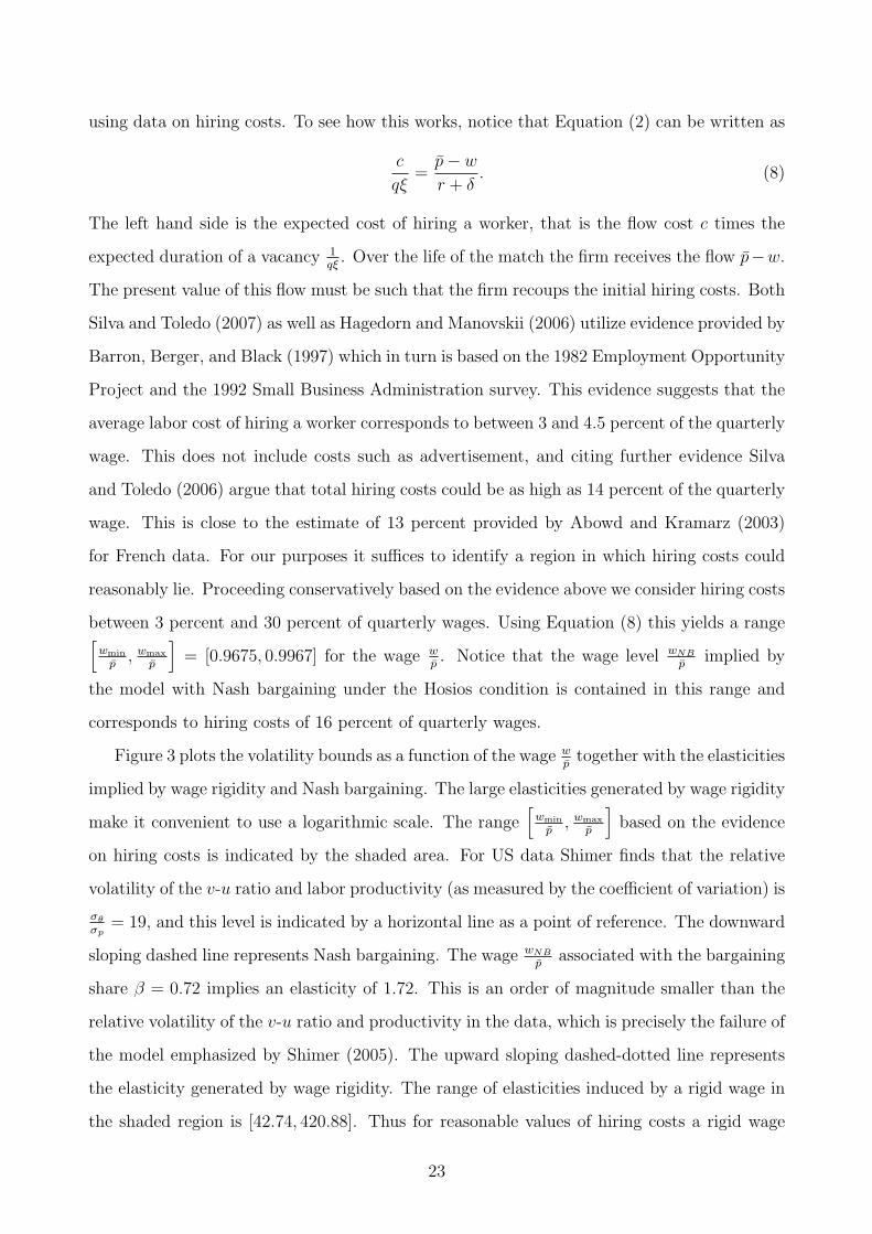
Figure 3 plots the volatility bounds as a function of the wage wp

together with the elasticities

implied by wage rigidity and Nash bargaining. The large elasticities generated by wage rigidity

make it convenient to use a logarithmic scale. The range[

wmin

p, wmax

p

]based on the evidence

on hiring costs is indicated by the shaded area. For US data Shimer finds that the relative

volatility of the v-u ratio and labor productivity (as measured by the coefficient of variation) is

σθ

σp= 19, and this level is indicated by a horizontal line as a point of reference. The downward

sloping dashed line represents Nash bargaining. The wage wNB

passociated with the bargaining

share β = 0.72 implies an elasticity of 1.72. This is an order of magnitude smaller than the

relative volatility of the v-u ratio and productivity in the data, which is precisely the failure of

the model emphasized by Shimer (2005). The upward sloping dashed-dotted line represents

the elasticity generated by wage rigidity. The range of elasticities induced by a rigid wage in

the shaded region is [42.74, 420.88]. Thus for reasonable values of hiring costs a rigid wage

23

Figure 3: Volatility Bounds

b = 0.4 0.6 0.8 1wp

1.72

6.82

19

50

100 εθ,HALL

εθ,WEAK

εθ,STRONG

εθ,NASH

generates an elasticity εθ in excess of the empirical relative volatility σθ

σp. This suggests that

wage rigidity generates more than enough amplification, leaving room for the possibility that a

weaker form of rigidity could suffice to match observed labor market volatility.14 In particular,

one may ask whether rent rigidity is capable of doing so.

A negative answer to this question is provided by the plots of the two volatility bounds.

Both are represented by solid lines, the strong bound with crosses. Over the shaded region of

interest the two bounds are quantitatively close and vary little: the weak bound ranges from

6.48 to 6.82 whereas the strong bound ranges from 5.88 to 6.38. Thus for reasonable values of

hiring costs, models of wage determination that generate procyclical worker rents can generate

at most a third of observed volatility.15 In other words, replacing Nash bargaining by a model

14 The range of elasticities [42.74, 420.88] overstates the case that a rigid wage generates more than enough

amplification. As discussed before, the case of permanent shocks provides an upper bound for the case in which

persistence is calibrated to US data. To investigate this issue we calibrated the rigid wage model following

the approach of Shimer (2005) for wage levels in the shaded range and obtained the range [20.8, 57.9] for the

relative coefficient of variation σθ

σp

µp

µθ. Thus it is still the case that a rigid wage generates relative volatility in

excess of what is observed.15 Mortensen and Nagypal (2005) argue that 7.52 is a more appropriate target for the elasticity εθ than

the value of 19 implicit in Shimer (2005). Their argument is based on the relatively low empirical correlation

24

with rigid rents does not provide a silver bullet for resolving the inability of the model to

match observed labor market fluctuations. Nevertheless, some amplification vis-a-vis Nash

bargaining is not ruled out by the bound. Thus it is of interest whether the bound can be

attained. We have already shown that the strong bound can be attained with complete rent

rigidity, and in Section 4 we show how it is attained by a model of wage determination under

asymmetric information.16

Notice that the two bounds coincide for wp

= 1. Recall that the difference between the

two bounds is that the weak bound neglects the congestion effect. This effect is zero for

wp

= 1. If the model is calibrated to a lower annuity value of wages wp

< 1, then a gap appears

between the two bounds. The weak bound increases as it only reflects the feedback effect,

whose strength is reduced if wages and thus worker rents are small. It asymptotes to infinity

because the feedback effect disappears as the annuity value of wages approaches the value of

non-market activity b. In contrast, the strong bound is an increasing function of the annuity

value of wages. Recall from Equation (7) that the strong bound is a weighted average of the

feedback and the congestion effect. The weight on the feedback effect is an increasing function

of the annuity value of wages. Thus the slope of the strong bound depends on which of the two

effects puts a tighter limit on labor market fluctuations. The plot shows that the congestion

effect is more severe: calibrating the model to match a lower annuity value of wages reduces

the amplification generated by rent rigidity. Setting w = b puts all weight on the congestion

effect and yields εθ,STRONG = p

p−b1

1−η= 2.31; putting all weight on the feedback effect by

setting w = p yields εθ,STRONG = p

p−b1η

r+δ+f

f= 6.45. Importantly, the strong bound is finite

between labor market tightness and labor productivity, suggesting that part of fluctuations in labor market

tightness is due to other shocks. Rent rigidity comes close to attaining their 7.52 target. Thus while rent

rigidity alone cannot enable the model solely driven by productivity shocks to match observed volatility, a

model with rigid rents and multiple shocks could get close. On the other hand, the appropriate target for εθ

could be even higher than Shimer’s 19 if the low empirical correlation between labor market tightness and

labor productivity reflects measurement error in the latter rather than other shocks.16That the model can attain the bound does not mean that the relative coefficient of variation σθ

σp

µp

µθfrom

simulations with productivity persistence calibrated to US data is necessarily close to the strong bound, for

the reason already discussed in Footnote 14. Simulating the model for the usual range of wages, following the

approach of Shimer (2005), yields yields the range [5.18, 6.30] for the relative coefficient of variation, compared

to the corresponding values for the bound [5.88, 6.38]. Thus the simulated model comes very close to attaining

bound.

25

irrespective of the annuity value of wages. In this sense it requires less empirical information

than the weak bound. In particular, using only parameters from Shimer’s calibration and

without calibrating hiring costs we can conclude that models of wage determination subject

to the strong bound cannot generate more than a third of observed volatility.

The congestion effect is maximized if the annuity value of wages w equals the value of

non-market activity. In this case Nash bargaining, rent rigidity and wage rigidity all coincide.

The plot of the strong bound illustrates that rent rigidity lies between Nash bargaining and

wage rigidity, but quantitatively it is much closer to the former (remember that the scale is

logarithmic).

Why does the congestion effect put a tighter limit on fluctuations than the feedback effect in

Shimer’s calibration? The size of the feedback effect is determined by the term 1η

r+δ+f

f. Since

f ≫ r + δ this is well approximated by 1η. The strength of the congestion effect is determined

by 11−η

. Thus which one of the two effects puts a tighter bound on amplification in essence

just depends on the matching function elasticity η. If η is below 12

as in Shimer’s calibration,

then an increase in the number of vacancies primarily causes congestion with little effect on

the job finding rate and a correspondingly weak feedback effect. If instead η is above 12

an

increase in vacancies is associated with a strong response of the number of matches, causing

little congestion while substantially increasing the job finding rate of unemployed workers.

Since the elasticity η plays such an important role it is useful to consider how changing this

parameter affects the bounds. This is particularly important since Shimer’s value lies at

the low end of the reasonable range of [0.3, 0.5] identified in the survey by Petrongolo and

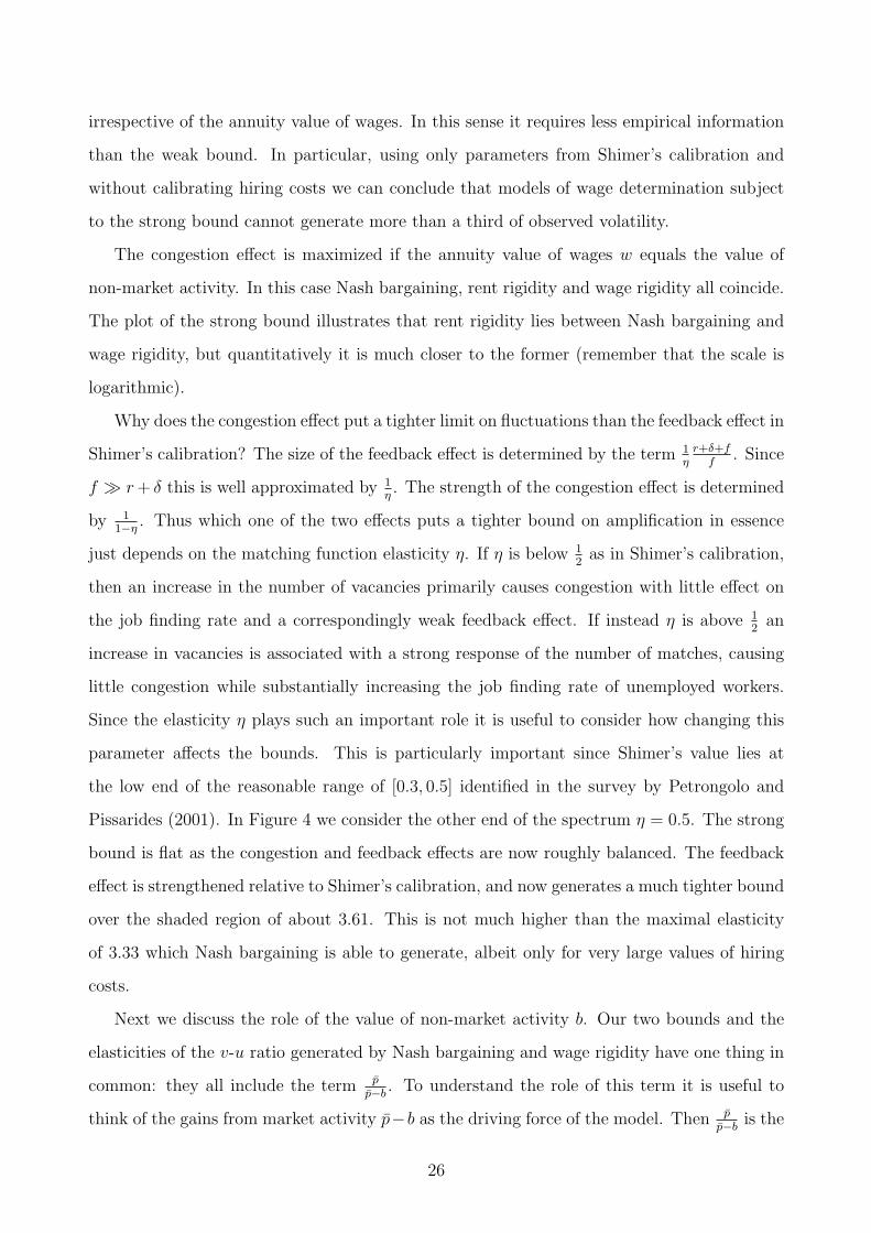
Pissarides (2001). In Figure 4 we consider the other end of the spectrum η = 0.5. The strong

bound is flat as the congestion and feedback effects are now roughly balanced. The feedback

effect is strengthened relative to Shimer’s calibration, and now generates a much tighter bound

over the shaded region of about 3.61. This is not much higher than the maximal elasticity

of 3.33 which Nash bargaining is able to generate, albeit only for very large values of hiring

costs.

Next we discuss the role of the value of non-market activity b. Our two bounds and the

elasticities of the v-u ratio generated by Nash bargaining and wage rigidity have one thing in

common: they all include the term p

p−b. To understand the role of this term it is useful to

think of the gains from market activity p−b as the driving force of the model. Then p

p−bis the

26

Figure 4: Volatility Bounds η = 0.5

b = 0.4 0.6 0.8 1wp

1.76

3.82

19

50

100εθ,HALL

εθ,WEAK

εθ,STRONG

εθ,NASH

elasticity of this driving force with respect to productivity. If b is close to p, then even small

fluctuations in productivity can generate large fluctuations in the driving force of the model.

Thus even if the model does not strongly amplify fluctuations in p − b it could still generate

large labor market fluctuations for sufficiently large b. In Shimer’s calibration p

p−b= 1.67

is small. Hagedorn and Manovskii (2006) show that with bp

= 0.955 even Nash bargaining

can match observed labor market fluctuations. Analogously one may ask: at what value of

non-market activity can the model of complete rent rigidity match observed volatility? For

an annuity value of wages wNB

p= 0.9826 the answer is b

p= 0.828.

4 Wage Determination under Asymmetric Information

We now consider classic models of bargaining with incomplete information, that have been

studied very extensively. We want to check whether these models exhibit the properties, such

as Increasing worker rents, under which the labor market volatility bounds apply. These are

comparative statics properties of equilibrium outcomes of the bargaining game. Comparative

statics are meaningful only when the equilibrium prediction is unique. Thus, we focus our

attention on bargaining protocols for which the literature has established outcome uniqueness,

27

possibly subject to appropriate refinements: one-sided offers with and without commitment

to the offer, strategic bargaining with one-sided asymmetric information, and the constrained

efficient allocation maximizing expected gains from trade. In each case, the comparative

statics properties of the unique equilibrium outcome are unknown, so we have to derive them

anew.

There is an additional reason to focus on unique outcomes. If the bargaining game has

multiple outcomes, then this could be exploited to generate amplification by selecting an

outcome favorable to firms in booms and an outcome favorable to workers in recessions.

However, asymmetric information is not needed to do this. In fact, Hall (2005) exploits

multiplicity in this way to provide a foundation for wage rigidity in the model with symmetric

information. He assumes that the wage is set through a double auction. The key feature of

the double auction under symmetric information environment is that any split of the gains

from trade is an equilibrium. Thus one can select the rigid wage as the equilibrium for all

combinations of p and n, as long as this wage is always in the bargaining set [n, p]. Since

multiplicity can be used to generate the observed amount of volatility even under symmetric

information, the only interesting question is whether models with asymmetric information are

capable of doing so without exploiting multiplicity. Hence our focus on bargaining protocols

with unique outcomes.

In our setting, private information concerns the idiosyncratic productivity component of

the match, y, and amenity value for the worker, z. The distributions FY and FZ have support

[y, y] and [z, z], respectively, with y, z, y, z ∈ R. We now introduce a standard technical

assumption about private information.

Assumption 1. (Monotone Virtual Valuations) The “virtual valuations” y − 1−FY (y)F ′

Y(y)

and z − 1−FZ(z)F ′

Z(z)

are strictly increasing and continuously differentiable on [y, y] and [z, z], re-

spectively.

For each of the rent-sharing models that we examine, we proceed as follows: we show that

Condition 1 (c) holds, and then that expected rents are a function of p and n only through

their difference p − n, with G ′(p − n) ≥ 0 and J ′(p − n) ≥ 0. This is all that we need for the

first bound to apply. In fact, it implies that

∂G

∂p= G ′(p − n) = −

∂G

∂n≥ 0

28

which implies Increasing worker rents and thereby Condition 1 (a). It also implies

−∂J

∂n= J ′(p − n) ≥ 0

which is Condition 1 (b). For the second bound, we also verify Condition 2 directly.

4.1 Monopoly

First, we consider the simplest game in which the privately uninformed party makes a take-

it-or-leave-it offer to the informed party. This is the model suggested by Shimer (2005) in

his conjecture that asymmetric information may generate amplification. In this model, the

relationship ends if the informed party rejects the offer. In other words, the uninformed party

can commit not to make another offer if its first offer is rejected. This game has a unique

equilibrium, which is constrained ex ante efficient in the sense that the offer-making party’s

welfare cannot be improved further given information asymmetry (Satterthwaite and Williams

(1989)). Yet, it does not maximize ex ante gains from trade, due to the monopoly distortion.

We analyze separately the two cases of unilateral wage offer by the firm and wage request

by the worker, because the properties used to derive the second bound are not symmetric for

firms and workers.

Take-It-or-Leave-It Wage Offer by the Firm. A firm of type y offers a wage wM to the

job applicant, who is then indifferent between accepting and rejecting it to stay unemployed

when his amenity value is exactly zM = n−wM . If z ≥ zM , and the offer is accepted, an event

with chance 1−FZ(zM), the firm earns flow profits p+y−wM = p−n+y+zM . Equivalently,

the firm chooses the threshold zM , rather than the wage wM , to maximize the PDV of:

[1 − FZ(zM)](p − n + y + zM). (9)

The well-known first order condition is

p − n + y + zM =1 − FZ(zM)

F ′Z(zM)

. (10)

The left hand side is the gain from trading with an additional worker. However, if the firm

wants to trade with more workers, it has to pay higher informational rents to the workers

(types, values of z) it is already trading with. The right hand side gives the number of

workers that receive higher rents relative to the number of workers gained from reducing zM .

29

If (10) has an interior solution zM(p−n+y), by Assumption 1, this is unique, differentiable,

and the global maximizer. Assumption 1 allows for finite lower and upper bounds, so zM(p−

n + y) could be at a corner, equal to the lower bound z (the offer is accepted for sure) if

p−n+y + z ≥ [F ′Z(z)]−1, that is if the gain from trading with more workers always outweighs

the cost of higher informational rents, and equal to the upper bound z (the offer is rejected

for sure) if p − n + y + z ≤ 0. One may expect that corner solutions may generate sufficient

wage rigidity to escape the bounds. We will show that this is not the case.

From acceptance of its offer, the firm learns that the type of the worker is at least zM(p−

n + y). Although it has obtained this information, the firm would not want to revise its wage

offer if it were allowed to do so.17 Thus the key assumption regarding commitment is not that

the firm can commit not to make a lower wage offer after acceptance, but that it can commit

not to make a higher wage offer after being rejected.

It is now straightforward to map this model of wage determination into the notation of

Section 2, and check that it satisfies the properties there introduced:

G(y, z, p, n) = x(y, z, p − n)z − zM(p − n + y)

r + δ,

J(y, z, p, n) = x(y, z, p − n)p − n + y + zM(p − n + y)

r + δ,

x(y, z, p − n) = I {z ≥ zM(p − n + y)} . (11)

The trade decision x depends on p and n only through their difference p−n. Moreover, the

same is true for the functions G and J and for their unconditional counterparts, that we can

write as ξ(p− n), G(p− n) and J (p− n) from now on. Inspecting the firm’s objective in (9),

an increase in p−n + y raises the marginal gain from trade by lowering the threshold zM . By

a monotone comparative statics argument, or by the implicit function theorem, zM(p−n+ y)

is weakly decreasing (and strictly so over the range where the solution is interior). Consulting

Equation (11), this implies that x(y, z, p−n) is non-decreasing in both y and z, and Condition

1 (c) is verified. As discussed earlier, for the first bound we just need G ′(p−n), J ′(p−n) ≥ 0.

Define the worker’s average gains from trading with a firm of type y:

(r + δ)G(p − n|y) ≡

∫ z

zM (p−n+y)

[z − zM(p − n + y)] dFZ(z).

17Formally, the objective of the firm facing the distribution of worker types truncated at zM (p − n + y) is

given by p−n+ y + zM for zM ≤ zM (p−n+ y) and 1−FZ(zM )1−FZ(zM (p−n+y)) (p−n+ y + zM ) for zM ≥ zM (p−n+ y).

The unique maximizer is still zM (p − n + y).

30

This function is differentiable everywhere, including at the two threshold values of y where

the first order condition (10) holds with equality for the corners z and z, with

(r + δ)G ′(p − n|y) = −z′M(p − n + y)[FZ(zM(p − n + y))] ≥ 0.

The firm expands the range of workers it is trading with by −z′M(p−n+y), so the informational

rents of all worker types that it is already trading with have to increase by exactly this amount.

If zM(p−n+y) is at a corner z or z, clearly z′M(p−n+y) = 0 and the inequality still applies.

By definition G(p − n) =∫G(p − n|y)dFY (y), so that

G ′(p − n) =

∫G ′(p − n|y)dFY (y) ≥ 0.

For the firm, the maximized value for type y is

(r + δ)J (p − n|y) = [1 − FZ(zM(p − n + y)) [p − n + y + zM(p − n + y)] .

Differentiation yields

(r + δ)J ′(p − n|y) = 1 − FZ(zM(p − n + y)).

If the firm is at a corner this follows immediately, as zM(p − n + y) does not respond to a

change in p−n. If the solution to the firm’s problem is interior, this relationship follows from

the envelope theorem. Since the threshold zM is chosen optimally, the firm cannot gain at

the margin from adjusting the threshold, so the benefit from an increase in p − n is just the

direct effect on the rents that the firm earns from the workers that it is already trading with.

It follows that J (p−n|y) is continuously differentiable, and differentiation under the integral

sign yields

(r + δ)J ′(p − n) =

∫(r + δ)J ′(p − n|y)dFY (y)

=

∫[1 − FZ(zM(p − n + y))]dFY (y) = ξ(p − n) ≥ 0.

This also establishes that Condition 2 holds with equality. Recall our discussion that Condition

2 is innocuous if trade is ex post efficient, because in this case the envelope theorem implies

(r + δ)(

∂G∂p

+ ∂J∂p

)= ξ. Here Condition 2 again follows from the envelope theorem which

delivers (r + δ)∂J∂p

= ξ. At the same time, due to the monopoly inefficiency, trade is generally

not ex post efficient (r + δ)(

∂G∂p

+ ∂J∂p

)> ξ.

We summarize these results in the following:

31

Proposition 3. Under Assumption 1 the model of wage determination through a take-it-

or-leave-it offer by the firm to a privately informed worker satisfies Conditions 1 and 2 and

Increasing worker rents. Thus, both labor market volatility bounds of Propositions 1 and 2

apply.

Take-It-or-Leave-It Wage Request by the Worker. By symmetry with the case that

we just analyzed, when the worker makes a take-it-or-leave-it wage request from the firm,

Condition 1 is satisfied and worker rents are Increasing. These are all the properties needed

to apply the weak bound of Proposition 1.

To apply the strong bound, we cannot invoke symmetry with the previous case: there, we

only established that the rents of the offer-making party satisfy Condition 2, while now the

firm is at the receiving end of the offer. Using notation symmetric to the firm offer model, in

the worker request model

(r + δ)J ′(p − n|z) = −y′M(p − n + z)[1 − FY (yM(p − n + z))] (12)

at points of differentiability of yM(p − n + z), the threshold productivity level chosen by

the worker with amenity value z. Only firm types that the worker has already been trading

with experience an increase in their informational rent, which is why the probability of trade

1−FY (yM(p− n + z)) appears in Equation (12). How large the increase in the informational

rent is for these firm types depends on how many more firm types the worker wants to trade

with, that is, on the drop in the threshold −y′M(p− n + z). If the worker reduces the request

and thus the feasible productivity threshold substantially, then the firm will experience a large

increase in its informational rents. Now suppose that the worker reduces the threshold less

than one for one with an increase in p − n, that is −y′M(p − n + z) ≤ 1. Then

(r + δ)J ′(p − n) =

∫−y′

M(p − n + z)[1 − FY (yM(p − n + z))]dFZ(z)

≤

∫[1 − FY (yM(p − n + z))]dFZ(z) = ξ(p − n),

enough for Condition 2. The following strengthening of the second part of Assumption 1

suffices for −y′M ≤ 1.

Assumption 2. (Monotone Hazard Rate) The hazard rateF ′

Y (y)

1−FY (y)is weakly increasing

and continuously differentiable on [y, y].

32

To understand the role of a monotone hazard rate, consult the worker’s first order condition

for an optimal wage request to the firm:

p − n + yM + z =1 − FY (yM)

F ′Y (yM)

.

If in response to an increase in p − n the worker reduced yM one for one, then the left hand

side, which is the marginal benefit from trading with another firm type, would be unchanged.

However, under Assumption 2 the worker would end up at a point with a lower hazard rate,

that is the loss of trade associated with a more aggressive wage request would be smaller

relative to the number of firms that would pay the higher wage. It follows that it is optimal

to reduce the threshold less than one for one.

Thus we obtain the following:

Proposition 4. Under Assumption 1 the model of wage determination through a take-it-or-

leave-it request by the worker to a privately informed firm satisfies Condition 1 and Increasing

worker rents. Thus, the weak labor market volatility bound of Proposition 1 applies. If As-

sumption 1 is strengthened to Assumption 2, then this model also satisfies Condition 2 and

the strong volatility bound of Proposition 2 also applies.

Kennan (2006) also considers the model with take-it-or-leave-it offers, and he is able to

generate large fluctuations in unemployment and vacancies. As discussed in the introduction,

his approach exploits asymmetric information in a different way from what we consider in this

paper. We ask how the presence of asymmetric information changes the response of the labor

market to an increase in aggregate labor productivity, but the extent of private information

itself is acyclical. In contrast, in Kennan (2006) exogenous fluctuations in the shape of the

distribution of types are the key driving force of labor market fluctuations. Specifically, he

assumes that the match specific productivity component can be either high or low, and that

the high value is more likely in booms. He assumes that parameters are such that pooling

occurs in both booms and recessions: workers always request the wage that makes the low

firm type indifferent. Since the value of unemployment is procyclical, it follows that worker

rents are countercyclical.18

18 Translated into our notation, in Kennan (2006) both p and FY vary over the cycle. It is straightforward

to decompose labor market volatility into three sources: p, FY , and an interaction term. In his calibration

33

In Section 3.2 we demonstrated that the strong labor market volatility bound can be

attained by the model of complete rent rigidity. We now show that there exist beliefs such

that the monopoly model also attains the bound.

Attaining the Strong Bound in Firm Offer Monopoly. The idea is to construct beliefs

such that the monopoly model maps exactly into the model of complete rent rigidity, that is

the worker receives a fixed flow rent g > 0. For simplicity there is no heterogeneity on the firm

side, that is FY is degenerate. Let w = b+ r+δ+f

r+δg. As in the model with complete rent rigidity,

this turns out to be the equilibrium annuity value of wages. Let j = p − w = p − b − r+δ+f

r+δg,

which will be the equilibrium value of profits. Consider beliefs

FZ(z) ≡1 − j

z+g+j

1 − j

z+g+j

with support [z, z] where the lower bound is z = −g and the upper bound is chosen to insure

a zero mean, that is it is the unique positive solution to the equation∫ z

zzFZ(dz) = 0. We will

show that in steady state the firm trades with all worker types. Steady state flow rents are

p−n = g + j. More importantly, we show that trading with all worker types remains optimal

in response to a productivity shock, which in turn implies G ′(g + j) = 0. Thus this example

maps exactly into the model of complete rent rigidity.

First note that if the firm chooses to trade with all worker types, then flow worker rents

are

(r + δ)

∫ z

z

(z − z)dFZ(z) = −z = g.

Furthermore, if flow worker rents are g, then equilibrium condition (3) implies that in equi-

librium p−n = g + j. Thus it remains to show that it is indeed optimal for the firm to choose

the lower bound z for a neighborhood around p − n = g + j. Evaluating the objective of the

firm at p − n = g + j yields

(1 − FZ(z))(p − n + z) = (1 − FZ(z))(z + g + j) =j

1 − j

z+g+j

(1 −

z + g + j

z + g + j

),

a strictly decreasing function of z.

While monopoly can attain the bound for some beliefs, this is not to say that it generically

leads to amplification vis-a-vis Nash bargaining. It is easy to construct beliefs such that the

fluctuations in FY alone generate about 85 percent of observed volatility in the v-u ratio, while the contribution

of p and of the interaction term are small.

34

response of the labor market to a productivity shock is muted. Indeed, in his conjecture

Shimer (2005) merely argues that the model breaks the direct link between labor productivity

and the v-u ratio by making the response to a productivity shock a function of the hazard

rate. Thus at least the model adds may degrees of freedom that one may expect should

enable the model to match observed volatility. Our results imply that this is not the case:

the degrees of freedom are not enough to generate amplification in excess of the strong labor

market volatility bound. Moreover, if one chooses the distribution of beliefs to maximize

amplification, one obtains precisely complete rent rigidity.

4.2 Strategic Bargaining with One-Sided Private Information

We now move away from the case of extreme commitment to a (take-it-or-leave-it) offer, and

towards repeated, strategic bargaining. The theory of sequential non-cooperative bargaining

with private information has produced compelling predictions only for the case of one-sided

asymmetric information, that we address first. In the two-sided case, the wealth of Bayesian

equilibria makes alternating-offer games problematic as tools of analysis, despite the realism

of the setup. In that case, we will consider the unique allocation that maximizes expected

gains from trade through a mediator.

We focus on some popular and natural extensive forms of the bargaining game. In the

previous subsection we analyzed the case of a unilateral offer with commitment to a privately

informed party. In that case, the private information of the offer-making party is irrelevant,

so that solution applies both to one-sided and two-sided asymmetric information. We showed

that our bounds apply. Therefore, we now assume that parties cannot commit to walk away

when the opponent declines its offer, but they can commit to their offer should it be accepted.

The only change in the environment is that information is private only on one side. To

fix ideas, assume that the firm is uninformed about z but the worker observes y. The parties

then enter a bargaining phase. The firm (uninformed party) makes the first wage offer w. If

this is accepted, from then until the (exogenous) end of the match the firm has flow profits

p+y−w, the worker has flow payoffs w+z−n, the total surplus is p+y+z−n. If negotiations

end unsuccessfully, the firm obtains zero and the worker obtains a flow value n. Fix numbers

β ∈ [0, 1], ρwork ≥ 0, ρfirm ≥ 0. If the first offer is declined, negotiations break down with

35

chance 1− e−(1−β)∆, continue with chance e−(1−β)∆ and, after a delay ∆ and with discounting

cost e−ρfirm∆, the worker makes a new wage request. Again, if this is declined by the firm,

negotiations break down with chance 1− e−β∆ and continue with complementary probability,

in which case payoffs are further discounted at rate e−ρwork∆. Notice then that the discount

rate after a firm offer is declined is effectively equal to 1−β +ρfirm, and after a worker offer is

declined it equals β + ρwork. We study Perfect Bayesian Nash Equilibria (PBE) when ∆ → 0.

This model nests several well-known models as special cases. First, let the uninformed

party i ∈ {work, firm} make the first offer. If the discount rate ρi that applies after the first

offer is infinite, we are back to the previous case of monopoly with commitment. Therefore,

from now on we assume ρi < ∞. We analyze first the simpler case where repeated offers are

effectively one-sided.

Coase Conjecture. Suppose again for illustration that the firm is uninformed and β =

ρwork = 0 ≤ ρfirm < ∞. In this case, any request by the worker can be rejected at no cost by

the firm, because negotiations continue for sure and there is no discounting after a worker’s

request is declined, but declining a firm’s offer implies an efficiency loss (1 − β > 0). Thus,

offers are effectively one-sided. This is the case of a monopolist (firm) selling a durable good

(job) to a buyer (worker) who has private information about his own valuation (z) for the job.

The firm (uninformed) makes the first offer. As is well-known, the unique PBE as ∆ → 0

dictates that negotiations end immediately and the worker extracts all rents from the firm,

the Coase Conjecture (Gul and Wilson (1986)). We now examine the properties of this model

of wage determination. We have two subcases.

In the Gap case the firm’s draw of match productivity y is such that there are gains from

trade for sure, p + y + z − n > 0. Then the sequential equilibrium wage of the subgame

following the observation of y is w(p, n, y) = n − z < p + y, all worker types accept if payoffs

are w + z − n = z − z > 0, the firm makes profits p + y − w = p − n + y + z > 0. In the

No-Gap case, given productivity y, gains from trade exist only for some worker types z, such

that p + y + z − n ≤ 0 < p + y + z − n. Then, the unique equilibrium satisfying a stationarity

condition on strategies has the following outcome. The wage offer w(p, n, y) = p+y is accepted

immediately, the firm is left with nothing, workers with z ≥ n − (p + y) accept and obtain

rents p + y + z − n, the other worker types decline.

36

Trade is ex post efficient, so the ex ante probability of trade is simply ξ(p − n) = Pr(p −

n + y + z ≥ 0) and Condition 1 (c) is verified. Notice that once again not only the trade

decision but also the split of rents depends on p and n only through their difference p − n.

We are left to verify G ′, J ′ ≥ 0. The firm’s rents are

(r + δ)J (p − n) = Ey,z [p + y − w(p, n, y)] =

∫ y

n−p−z

(p − n + y + z) dFY (y)

with

(r + δ)J ′(p − n) = 1 − FY (n − p − z) ∈ [0, ξ(p − n)]

implying Conditions 1 (b) and 2. The fact that trade is ex post efficient implies that (r +

δ)(G ′ + J ′) = ξ, so it immediately follows that (r + δ)G ′ ∈ [0, ξ]. Therefore, the worker and

firm informational rents have symmetric properties, and we can swap their roles. These facts

establish:

Proposition 5. Under Assumption 1 the “Coase Conjecture” model of wage determination

through quickly repeated unilateral offers by the uninformed party in stationary strategies satis-

fies Conditions 1 and 2 and Increasing worker rents. Thus, the labor market volatility bounds

of Propositions 1 and 2 apply.

Menzio (2005b) proposes a model of wage determination that delivers the same implications

as the Coase conjecture, albeit through a different mechanism. In his model workers are

uninformed. As under the Coase conjecture, the wage requested by the worker in equilibrium

is given by the productivity of the lowest firm type: w = p + y. The mechanism is as follows.

The firm employs many workers. If the firm grants a wage in excess of p + y to one worker,

then all its other employees learn that the firm’s type is higher than y, and they successfully

request wage increases. This spillover of information enables the firm to reject wage requests

in excess of p + y. As the implied wage is the same as under the Coase conjecture, it follows

that the labor market volatility bounds apply to this model of wage determination as well, as

long as private information is acyclical as it is assumed to be here. Menzio uses this model to

generate rigid wages as follows. He assumes that the lower bound of the distribution of firm

productivity is acyclical. Translated into our notation, p + y remains constant over the cycle.

As aggregate labor productivity is higher in booms while the lower bound is acyclical, it must

be that the shape of the distribution FY is changing over the cycle. Thus Menzio’s approach

37

is similar to Kennan (2006) in the sense that it relies on exogenous fluctuations in the shape

of the distribution of types in order to generate large labor market fluctuations.

Alternating Offers. Now suppose that β ∈ (0, 1), so declining an offer can always lead to

a breakdown in negotiations, and ρfirm = ρwork = r ≥ 0. These assumptions provide some

physical commitment to parties to walk away after receiving a negative answer to an offer, and

enhance the bargaining power of the uninformed party. We illustrate equilibrium predictions

drawing from Grossman and Perry (1986), Gul and Sonnenschein (1988), and Menzio (2005a).

In this game, Stationarity of equilibrium strategies is not sufficient to pin down a unique

PBE, and one needs to impose also a Monotonicity requirement on beliefs. Then, the unique

PBE is similar to the Coase conjecture, with the only twist that β measures the bargaining

power of the worker. That is, suppose now (for the sake of variety) that the firm is privately

informed about y, while z is common knowledge and the worker of type z makes the first

wage request. Then, in the Gap case, p+y+z − n > 0, the unique PBE wage first requested

by the worker of type z (and accepted by all firms) is w(p, n, z) = β(p+y) + (1 − β)(n − z)

and the worker obtains payoff z − n + w = β(p+y+z − n). That is, the wage must reflect

the worker’s valuation because with some probability (decreasing in β): negotiations break

down, the firm does not get its turn to counteroffer and it loses everything. This makes the

firm more willing to accept a high wage requests, the more so the higher β. The firm earns

p + y − w(p, n, z) = y − βy + (1 − β)(p − n + z). In the No-Gap case, the worker requests

w(p, n, z) = β(p + n − p − z)+ (1 − β)(n − z) = n − z and is left with zero payoffs, the firm

accepts if y ≥ n−p−z and earns p+y−w(p, n, z) = p+y−n+z. So the outcome is different

from that of one-sided repeated offers only in the Gap case.

The chance of trading ξ(p−n) is the same as in the previous model, so it satisfies Condition

1 (c), and

(r + δ)G(p − n) = β

∫ z

n−p−y

(p + y + z − n)dFZ(z).

Hence

(r + δ)G ′(p − n) = β[1 − FZ(n − p − y)

]∈ (0, ξ(p − n)) .

By the ex post efficiency of trade, this implies (r + δ)J ′(p−n) = ξ(p−n)− (r + δ)G ′(p−n) ∈

(0, ξ(p − n)). Again, these are the desired properties and are symmetric. We conclude:

38

Proposition 6. Under Assumption 1 the model of wage determination through quickly re-

peated alternating offers between an uninformed and an informed party, in stationary strate-

gies and monotone beliefs, satisfies Conditions 1 and 2 and Increasing worker rents. Thus,

both labor market volatility bounds of Propositions 1 and 2 apply.

4.3 Two-Sided Private Information: Constrained Efficient Alloca-

tion

The theory of strategic bargaining in the presence of bilateral asymmetric information, whether

with one-sided or alternating offers, has not produced compelling (unique) predictions based

on the Perfect Bayes Nash equilibrium notion even after restricting the space of strategies

by requirements such as stationarity of strategies and monotonicity of beliefs. The wealth of

reasonable off-equilibrium beliefs simply sustains many robust equilibria, even after applying

additional refinements.

We then turn to the constrained efficient allocation that maximizes expected gains from

trade, as in Myerson and Satterthwaite (1983), henceforth MS83. This corresponds to the

efficient allocation where both parties receive equal weight in the welfare function. Parties have

access to a mediator, who receives announcements about the draws of private information, y

and z, and recommends a binding allocation: a trading decision and a wage. After learning

their type, parties are willing to participate in the mechanism and truthfully reveal their

types. In this wage negotiation context, the mediator enforcing the rules of the game can be

thought of as an arbitrator of a labor dispute. The resulting constrained efficient allocation

can be implemented with a multiplicity of payment functions, but importantly it produces a

unique sharing of expected rents. This allocation is of great interest for its uniqueness, which

allows us to apply our test, and for two additional reasons: it features the maximal expected

gains from trade in the equilibrium of any unmediated bargaining game and, for some classes

of belief distributions, it can be implemented through a sealed-bid double auction. In this

subsection, we show that our weak bound from Proposition 1 applies to this allocation too.

We have not been able to either establish or disprove Condition 2 and the strong bound.

The Mechanism Design Problem. A mediator, or principal, receives reports y and z by

the two parties and enforces a probability of trade x(y, z, p, n) and a wage w(y, z, p, n) so as

39

to maximize the sum of expected values to the two parties. The reports are a Bayesian Nash

equilibrium of this optimal mechanism. That is, the efficient mechanism is a direct revelation

game whose Bayesian Nash equilibrium produces the constrained efficient allocation.

Given a pair of reports y, z and realizations y, z, the firm’s value is

(r + δ)J(y, z, y, p, n) = p + y − w(y, z, p, n)

and the worker’s value is

(r + δ)W (y, z, z, p, n) = z + w(y, z, p, n) + δU = z + w(y, z, p, n) + δn

r.

The constrained efficient allocation obtained through a direct revelation mechanism max-

imizes the total expected value to firm and worker

maxx,w

∫ z

z

∫ y

y

[J(y, z, y, p, n) + W (y, z, z, p, n)] x(y, z, p, n)dFY (y)dFZ (z)

+

∫ z

z

∫ y

y

U [1 − x(y, z, p, n)] dFY (y)dFZ (z)

subject to (interim) Individual Rationality (IR) and Incentive Compatibility (IC) constraints

of the firm: for all y, y ∈ [y, y]

∫ z

z

J(y, z, y, p, n)x(y, z, p, n)dFZ (z) ≥ max

⟨0,

∫ z

z

J(y, z, y, p, n)x (y, z) dFZ (z)

⟩

and of the worker: for all z, z ∈ [z, z]

∫ y

y

{W (y, z, z, p, n)x(y, z, p, n) + U [1 − x(y, z, p, n)]} dFY (y)

≥ max

⟨U,

∫ y

y

{W (y, z, z, p, n)x(y, z) + U [1 − x(y, z, p, n)]} dFY (y)

⟩.

Notice that this is not a constrained efficient allocation for society: here parties take the

outside option n = rU as given, and just mind the division of rents. The objective function is

independent of the wage w, which only plays the role of a transfer function to induce parties to

truthfully reveal their valuations, thus only enters the IC and IR constraints. In the appendix

we prove:

Lemma 7. Under Assumption 1, there exists a unique constrained efficient trading rule: trade

iff y ≥ y∗(z, p − n) where the decreasing function y∗ = y∗(z, p − n) uniquely solves

y∗ + p − n + z =µ

1 + µ

{1 − FY (y∗)

F ′Y (y∗)

+1 − FZ (z)

F ′Z (z)

}(13)

40

and µ ≥ 0 is the Lagrange multiplier on the constraint

∫ z

z

∫ y

y∗(z,p−n)

[p + y + z − n −

1 − FY (y)

F ′Y (y)

−1 − FZ (z)

F ′Z (z)

]dFY (y)dFZ (z) ≥ 0

which is equivalent to all IC and IR constraints.

The ex post probability of trade is x∗(y, z, p − n) = I{y ≥ y∗(z, p − n)} and the ex ante

chance of trade, unconditional on private information, is

ξ∗(p − n) =

∫ z

z

[1 − FY (y∗(z, p − n))]dFZ(z) =

∫ y

y

[1 − FZ(z∗(y, p − n))]dFY (y). (14)

Corner solutions are encompassed: if y∗(z) <y for some worker type z, this and all higher

types z′ > z who like the job even better than z are sure to trade. Conversely if y∗(z) > y for

some worker type z, this and all lower types z′ < z who like the job even less than z are sure

not to trade. Notice that the ex post efficient trading rule, trade iff y + p − n + z ≥ 0, holds

if and only if the constraint is not binding, or µ = 0. This happens in the Gap case, when

p − n is large enough that the supports of p + y and z − n are disjoint.

We can also state the constrained efficient trading rule in terms of the worker’s private

value: trade occurs iff z ≥ z∗(y, p − n) = y∗−1(y, p − n). Either way, the higher the valuation

a party has for the match, the more likely she expects trade to be. By the implicit function

theorem, these cutoff functions y∗ and z∗ are also differentiable in p − n. We now move to

verify the conditions stated at the beginning of this Section 4.

Expected Rents. As shown in MS83, the expected value to each party, unconditional on

trade but conditional on private information, can be written as

(r + δ)G∗(z|p, n) = (r + δ)G∗(z|p, n) +

∫ z

z

[1 − FY (y∗(z′, p − n))] dz′

(r + δ)J ∗(y|p, n) = (r + δ)J ∗(y|p, n) +

∫ y

y

[1 − FZ (z∗(y′, p − n))]dy′.

Notice that G∗(z|p, n) is increasing in z and J ∗(y|p, n) is increasing in y, so the IR constraints

G∗(z|p, n) ≥ 0 and J ∗(y|p, n) ≥ 0 for each type of worker and firm are satisfied if they are for

the lowest types y and z. By Theorem 2 in MS83, these are binding at the optimum:

G∗(p, n|z) = J ∗(p, n|y) = 0.

41

Taking expectations w.r. to private information, we obtain the expected values to each party

unconditional on trade and on private information. In the second and fourth equalities we

use integration by parts:

(r + δ)G∗(p − n) =

∫ z

z

∫ z

z

[1 − FY (y∗(z′, p − n))] dz′F ′Z(z)dz

=

∫ z

z

[1 − FY (y∗(z, p − n))] [1 − FZ(z)] dz

=

∫ z

z

∫ y

y

F ′Y (y)dy [1 − FZ(z)] x∗(y, z, p, n)dz

=

∫ y

y

F ′Y (y)

∫ z

z∗(y,p−n)

[1 − FZ(z)] dzdy

=

∫ y

y

∫ z

z∗(y,p−n)

(z − z∗(y, p − n))F ′Z(z)F ′

Y (y)dzdy.

Similarly

(r + δ)J ∗(p − n) =

∫ z

z

∫ y

y∗(z,p−n)

(y − y∗(z, p − n))F ′Y (y)F ′

Z(z)dzdy.

Notice the analogy with the monopoly model: a trading party enjoys expected rents equal to

the expected difference between its own valuation and the minimum acceptable valuation for

trade.

These rents are uniquely defined by the trading rule y∗, that we proved to uniquely exist,

and do not depend on the payment function w∗, which is defined residually. Therefore, G∗ and

J ∗ are uniquely defined as functions of p − n only.

Verifying the Conditions. Lemma 7 immediately implies Condition 1 (c). In the Appen-

dix, we prove the key result:

Lemma 8. G∗′(p − n) ≥ 0.

Since the roles of the worker and the firm in the mechanism design problem are symmetric,

as long as both distributions of types satisfy Assumption 1, we also obtain J ∗′(p − n) ≥ 0.

Intuitively, when the average gains from trade p − n rise, the mediator optimally re-adjusts

his mechanism so as to spread the benefits across both parties. One might expect that, in

situations where private information is lopsided and the IC constraint is much more binding for

one party, larger gains from trade p−n might be used by the mediator to relax that constraint

42

and to greatly increase the chance of trade. This may require reducing the expected payoffs

to the other party. Lemma 8 shows that this is impossible. Under bilateral asymmetric

information satisfying Assumption 1, labor market fluctuations of the empirically observed

magnitude are a symptom of wage-setting institutions that, albeit not necessarily privately

inefficient in the Pareto sense, do not fully exploit all possible gains from trade.

Proposition 9. Under bilateral asymmetric information satisfying Assumption 1, the con-

strained efficient model of wage determination, in which a mediator maximizes ex ante expected

gains from trade, satisfies Condition 1 and Increasing worker rents. Therefore, the labor mar-

ket volatility bound of Proposition 1 applies.

4.4 Summary

There are essentially two kinds of allocations that emerge in the games that we considered.

Either one party is left with no rents, as in the Coase conjecture, or an interior trading

cutoff on private information is chosen to maximize the rents of one or both parties, as in

the models of take-it-or-leave-it offers and the constrained efficient allocation. In the former

case, our conditions apply trivially. In the latter, they follow in part from an implication of

optimality, the envelope theorem.

The various models that we analyzed suggest a connection between private (in)efficiency

of wage setting and labor market volatility. To this purpose, it is useful to describe the Pareto

frontier under bilateral asymmetric information, interim participation and incentive compat-

ibility constraints. Barring transfers between parties at the ex ante stage, the constrained

efficient allocation is just one point on this frontier, right in the middle of it where both

parties receive equal weights. The extreme points of the frontier correspond to take-it-or-

leave-it offers, where one party obtains all the weight. Although the entire frontier of this

trading problem has not been fully characterized, in these three benchmark cases (points on

the frontier) either one or both of our bounds apply. We conjecture that all the allocations

on the frontier, for any given Pareto weights that do not change with aggregate productivity

p, satisfy our conditions for volatility bounds. Verifying this conjecture is a task for future

research. Some of the strategic bargaining models that we considered feature inefficiency but

no amplification, so inefficiency in wage setting may be necessary but is certainly not sufficient

43

for amplification of aggregate labor productivity shocks.

For belief distributions that give rise to linear “virtual valuations” (as defined in Assump-

tion 1) the unique constrained efficient allocation can be implemented through a sealed-bid

double auction (Satterthwaite and Williams 1989), the same mechanism as in Hall (2005), but

cannot provide the desired amplification. Yet, the double auction with two-sided asymmetric

information has multiple equilibria that are privately Pareto undominated, although they do

not maximize average gains from trade. Therefore, Hall’s mechanism, based on an appropriate

selection from the set of Pareto undominated equilibria, might still deliver the desired wage

rigidity and amplification with private information. Verifying this conjecture is difficult, for

two reasons. First, any amount of asymmetric information restricts the equilibrium set of the

double-auction, relative to the latitude exploited by Hall in the complete information case.

Second, the literature has not found a complete characterization of this equilibrium set. So

we leave also this conjecture for future research.

5 Transitory Aggregate Productivity Shocks

We have justified our focus on permanent productivity shocks claiming that labor market

volatility is even smaller if shocks are transitory. Thus the labor market volatility bounds

should still apply if shocks are not fully permanent. In this section we show that this is the

case, generalizing the labor market volatility bounds to an economy that switches between a

high state pH and a low state pL of aggregate labor productivity. Transitions from the high

state to the low state occur at rate λL, reverse transitions at rate λH . As an illustration

we generalize the firm offer monopoly model to this environment and demonstrate that the

bounds apply.

The equilibrium conditions now read

c

q(θH)= J H(pH , nH , pL, nL),

c

q(θH)= J L(pH , nH , pL, nL),

(15)

for free entry and

nH = b + θHq(θH)GH(pH , nH , pL, nL),

nL = b + θLq(θL)GL(pH , nH , pL, nL).(16)

44

for the opportunity cost of the worker.19 A model of wage determination is now a sextuple

{GH , GL, JH , JL, xH , xL} where for instance GH(y, z, pH , pL, nH , nL) is the initial worker rent

from a match formed in a high aggregate state with idiosyncratic productivity component y

and amenity value z. Worker rents of matches created in the high state depend on pL and nL

because labor productivity is no longer completely persistent and the match may eventually

find itself in the low state. The probability of trade is now a more complicated object. Let

h(s) denote the history of a match of age s. It includes the history of the aggregate state

and the history of trade within the match between match formation and the time at which

it reaches age s. Then xH(y, z, pH , nH , pL, nL, h(s)) denotes the probability of trade at age

s after history h(s). The sum GH + JH is the joint present value of the match induced by

the trade probability xH . The ex ante functions GH , GL, J H , J L are defined analogously to

Equation (1). Thus GH(pH , nH , pL, nL) is the ex ante worker rent of a match created in the

high aggregate state. We make the natural assumption that for identical states pH = pL and

nH = nL the model maps into the case we already studied: rents do not depend on the state

in which the match is created and the probability of trade is independent of history, so we

can define:

G(y, z, p, n) ≡ GH(y, z, p, n, p, n) = GL(y, z, p, n, p, n),

J(y, z, p, n) ≡ JH(y, z, p, n, p, n) = JL(y, z, p, n, p, n),

x(y, z, p, n) ≡ xH(y, z, p, n, p, n, h(s)) = xL(y, z, p, n, p, n, h(s)),

(17)

and Equation (1) yields the corresponding ex ante functions G, J and ξ.

For the case of permanent shocks we derived upper bounds on the elasticity of the v-u ratio

with respect to aggregate labor productivity p. Analogously, here we derive upper bounds on

the relative coefficient of variation of the v-u ratio and aggregate labor productivity σθ

σp

µp

µθ. In

the two state model the coefficient of variation for the v-u ratio can be written as

σθ

µθ

=

√λH

λH + λL

(λL

λH + λL

)2

+λL

λH + λL

(λH

λH + λL

)2θH − θL

λH

λH+λL θH + λL

λH+λL θL, (18)

19In standard notation Equation (16) for the high state reads

rUH = b + θHq(θH)GH(pH , nH , pL, nL) + λL(UL − UH).

Thus here nH = rUH − λL(UL − UH) and by symmetry nL = rUL − λH(UH − UL). As before

GH(pH , nH , pL, nL) = WH(pH , nH , pL, nL) − UH where WH(pH , nH , pL, nL) is the utility of a worker in

a job created in the high state.

45

and an analogous formula holds for the coefficient of variation of productivity σp

µp. Next we

provide the natural generalization of Condition 1 for this environment.

Condition 1′. The model of wage determination {GH , GL, JH , JL, xH , xL} satisfies three

properties:

(a) The partial effect of aggregate labor productivity in the high state pH on the difference

in worker rents across states is non-negative

∂GH

∂pH−

∂GL

∂pH≥ 0.

(b) The partial effect of worker’s opportunity cost in the high states nH on the difference in

firm rents across states is non-positive

∂J H

∂nH−

∂J L

∂nH≤ 0.

(c) The trade probabilities xH and xL depend on pH and nH only through their difference

pH − nH , on pL and nL only through their difference pL − nL, and are weakly increasing

in both match-specific outcomes, the firm’s idiosyncratic productivity y and the worker’s

amenity value for the job z.

To see that this is a generalization of Condition 1, consider for instance part (a). Suppose

productivity shocks are permanent. Then ∂GL

∂pH = 0: productivity in the high state is irrelevant

for rents in the low state as the low state lasts forever. Moreover ∂GH

∂pH = ∂G∂pH because the high

state lasts forever. Thus Condition 1′ (a) reduces to Condition 1 (a) if productivity shocks

are permanent.

5.1 Weak Labor Market Volatility Bound

To derive the weak bound we also need a generalization of Increasing worker rents.

Definition 1′. (Increasing Worker Rents) In a model of wage determination

{GH , GL, JH , JL, xH , xL} worker rents are Increasing if

∂GH

∂pH−

∂GL

∂pH≥ −

(∂GH

∂nH−

∂GL

∂nH

)≥ 0.

46

Our approach to deriving the bounds in this setting is as follows. As before we consider

small productivity shocks. Specifically, we linearize the model around a steady state with

productivity p. That is, the two productivity values pH , pL must satisfy λH

λH+λL pH + λH

λH+λL pH =

p. Importantly, with respect to the transition rates λH and λL we provide an upper bound,

that is the bounds apply not only if λH and λL are close to zero, but for any values of λH and

λL.

First we note a fact that will be convenient in the linearization. In what follows all

derivatives are evaluated at (p, n, p, n) where n is the steady state opportunity cost of the

worker induced by productivity p. Identity (17) yields

∂J H

∂pH+

∂J H

∂pL=

∂J L

∂pH+

∂J L

∂pL,

and an analogous relationship holds among the derivatives of GH and GL. These relationships

allow us to compactly write the linearization of the model using only the derivatives with

respect to productivity pH and opportunity cost nH in the high state. Linearizing the model,

we obtain

(1 − η)JθH − θL

θ=

(∂J H

∂pH−

∂J L

∂pH

)(pH − pL) +

(∂J H

∂nH−

∂J L

∂nH

)(nH − nL) (19)

from Equation (15) and

nH −nL = ηf

ξG

θH − θL

θ+

f

ξ

[(∂GH

∂pH−

∂GL

∂pH

)(pH − pL) +

(∂GH

∂nH−

∂GL

∂nH

)(nH − nL)

](20)

from Equation (16). The second term on the right hand side of Equation (20) capture the

change in worker rents. This leads to the following definition of procyclical worker rents for

the linearized model:

Definition 2′. (Procyclical Worker Rents) Worker rents are Procyclical in equilibrium

if (∂GH

∂pH−

∂GL

∂pH

)(pH − pL) +

(∂GH

∂nH−

∂GL

∂nH

)(nH − nL) ≥ 0.

In the appendix we prove the following version of Proposition 1 for the linearized model:

Proposition 1′. (Weak Volatility Bound) If the model of wage determination satisfies

Condition 1′ and worker rents are Procyclical, then σθ

σp

µp

µθ≤ εθ,WEAK. If worker rents are

Increasing, then they are Procyclical.

47

5.2 Strong Labor Market Volatility Bound

For the strong bound a generalization of Condition 2 is needed.

Condition 2′. In a model of wage determination {GH , GL, JH , JL, xH , xL} firm rents satisfy

the property

(r + δ)

(∂J H

∂pH−

∂J L

∂pH

)(p, n, p, n) ≤ ξ(p, n).

In the appendix we prove the following for the linearized model:

Proposition 2′. (Strong Volatility Bound) If the model of wage determination satisfies

Conditions 1′ and 2′ and if worker rents are Increasing, then σθ

σp

µp

µθ≤ εθ,STRONG.

5.3 Monopoly

We consider take-it-or-leave-it offers by the firm and analyze the case without firm hetero-

geneity for simplicity. Again the firm has the power to commit not to make further offers to

workers that have rejected an offer. It does not matter whether the firm also can commit not

to make further offer to workers who accepted an offer. Thus we could assume that the firm

makes a take-it-or-leave-it offer of a contract which specifies wage payments conditional on the

history of the aggregate state, and has the ability to commit to this contract. Or we could let

the firm change the wage whenever it finds it optimal to do so (but importantly, never makes

a follow up offer to workers who reject a wage change). Both cases lead to the same outcome,

which takes the following form. First consider a match created in the low state. Optimal firm

offers yield the firm rent

(r + δ)J L(pH , nH , pL, nL) =1

r + δ + λH + λL

· maxz

[(r + δ + λL)(1 − FZ(z))

(pL − nL + z

)+ λH(1 − FZ(z))

(pH − nH + z

)].

To understand this expression, recall that in the absence of transitions between the two states,

the firm would like to trade with more worker types in the high state. Here the firm starts in

the low state, but expects the match to be in the high state for part of its duration. In this

situation it is not optimal to hire workers only up to the point where profits in the low state

(1− FZ(z))(pL − nL + z

)are maximized, because this constrains the set of worker types the

firm can trade with once the boom comes. This consideration leads to a kind of labor hoarding:

48

the cutoff chosen by the firm, denoted by zLM(pH − nH , pL − nL), strikes a balance between

the time the match spends in the two states, which is captured by the weights r + δ + λL and

λH .

The situation is somewhat different for a match created in the high state. The reason is

that hiring many worker types does not put a binding constraint on the set of worker types

the firm wants to trade with once the slump comes, because in the slump the firm actually

wants to shed worker types. Thus when a match is created in a boom, it is optimal to hire

worker types up to the point where profits in the high state (1 − FZ(z))(pH − nH + z

)are

maximized. Let zM(pH −nH) denote the corresponding cutoff. Once the match enters a slump

for the first time, it is essentially the same as a match created in the slump, and it is optimal

to shed workers below the threshold zLM(pH − nH , pL − nL). Thus the firm rent is given by

(r + δ + λL)J H(pH , nH , pL, nL) = maxz

[(1 − FZ(z))

(pH − nH + z

)]+ λLJ L(pH , nH , pL, nL).

This behavior of the firm generates worker rents

(r + δ)GL(pH , nH , pL, nL) =

∫ z

zbM

(pH−nH ,pL−nL)

[z − zb

M(pH − nH , pL − nL)]dFZ(z),

GH(pH , nH , pL, nL) =1

r + δ + λL

∫ z

zM (pH−nH)

[z − zM(pH − nH)

]dFZ(z)

+λL

r + δ + λLGL(pH , nH , pL, nL).

Having derived firm and worker rents for this model of wage determination, we now show

that both the weak and the strong bound apply. Condition 1′ (c) is clearly satisfied, as trade

follows a cutoff rule, and the cutoffs depend on pH , nH , pL and nL only trough the differences

pH − nH and pL − nL. Next we verify Condition 1′ (b) along with Condition 2′. We have

(r + δ)∂J L

∂pH(p, n, p, n) =

λH

r + δ + λH + λL(1 − FZ(zM(p − n))) =

λH

r + δ + λH + λLξ(p, n)

where we exploit the fact that zLM(p−n, p−n) = zM(p−n). Differentiating J H with respect

to pH and combining results then yields

(r + δ)

(∂J H

∂pH−

∂J L

∂pH

)(p, n, p, n) =

r + δ

r + δ + λH + λLξ(p, n). (21)

This verifies Condition 2′. Recall that with permanent shocks Condition 2 holds with equality.

Equation (21) is consistent with this result as the right hand side reduces to ξ(p − n) for

49

λH = λL = 0. But with λH > 0 or λL > 0 there is some slack: fluctuations in firm rents

across states and thereby labor market volatility are smaller if aggregate productivity shocks

are more transient. Condition 1′ (b) immediately follows as ∂JH

∂nH − ∂JL

∂nH = −(

∂JH

∂pH − ∂JL

∂pH

).

It remains to show that worker rents are Increasing. Since ∂GH

∂nH − ∂GL

∂nH = −(

∂GH

∂pH − ∂GL

∂pH

)it

is enough to show that ∂GH

∂pH − ∂GL

∂pH ≥ 0. We have

(∂GH

∂pH−

∂GL

∂pH

)(p, n, p, n) =

ξ(p − n)

r + δ + λL

[∂zL

M

∂(pH − nH)(p − n, p − n) −

∂zM

∂(p − n)(p − n)

].

Rents in the high state respond more to an increase in pH than rents in the low state if the

threshold zM declines more than the threshold zLM . Differentiating the first order condition

implicitly defining zLM

r + δ + λL

r + δ + λH + λL(pL − nL) +

λH

r + δ + λH + λL(pH − nH) + zL

M =1 − FZ(zH

M)

fZ(zHM)

with respect to pH yields

∂zLM

∂(pH − nH)(p − n, p − n) = −

λH

r + δ + λH + λL

[1 −

(d

dz

1 − FZ(z)

fZ(z)

)∣∣∣∣z=zM (p−n)

]−1

.

Thus the response of zLM is proportional to the fraction of time the match spends in the high

aggregate state. Since zM does not put any weight on the low aggregate state it declines more

strongly

∂zM

∂(p − n)(p − n) = −

[1 −

(d

dz

1 − FZ(z)

fZ(z)

)∣∣∣∣z=zM (p−n)

]−1

and it follows that worker rents are Increasing.

Proposition 3′. Under Assumption 1 the model of wage determination through a take-it-or-

leave-it offer by the firm to a privately informed worker satisfies Conditions 1′ and 2′ and

Increasing worker rents. Thus, both labor market volatility bounds of Propositions 1′ and 2′

apply.

6 Conclusion

In this paper we have made two contributions to the debate on whether modifications to the

model of wage determination allow the search and matching model to generate larger labor

market fluctuations in response to productivity shocks. First, we have shown that models of

50

wage determination that cannot generate countercyclical rents, and thus at best generate rent

rigidity, are subject to labor market volatility bounds which are quantitatively tight. The

extent of amplification generated by rent rigidity is thus quite limited, and quantitatively rent

rigidity is much closer to Nash bargaining than it is to wage rigidity. Second, for a sequence of

classic models of wage determination under asymmetric information we have shown that rents

are not countercyclical. Thus a model with asymmetric information in which merely rents are

rigid cannot be the silver bullet which allows the search and matching model to match the

magnitude of observed fluctuations in unemployment and vacancies. Allowing the model to do

so solely through a modification of wage determination forces one to consider models that can

generate countercyclical rents. On the other hand, rent rigidity can generate a limited but not

insignificant amount of amplification. A full answer to Shimer’s (2005) findings may involve

more than one modification of the baseline model, of which a model of wage determination

with rigid rents could be one.

References

Abowd, J.M., and F. Kramarz. 2003. “The Costs of Hiring and Separations.” Labour

Economics 10 (5): 499–530.

Barron, J. M., M. C. Berger, and D. A. Black. 1997. On-the-Job Training. Kalamazoo, MI:

Upjohn Foundation for Employment Research.

Binmore, K., A. Rubinstein, and A. Wolinsky. 1986. “The Nash Bargaining Solution in

Economic Modeling.” RAND Journal of Economics 17 (2): 176–188.

Costain, J. S., and M. Reiter. 2005. “Business Cycles, Unemployment, and the Calibration

of Matching Models.” Working paper 872, Universitat Pompeu Fabra.

Grossman, S., and M. Perry. 1986. “Perfect Sequential Equilibrium.” Journal of Economic

Theory 39:97–119.

Guerrieri, V. 2006. “Heterogeneity and Unemployment Volatility.” mimeo.

Gul, F., and H. Sonnenschein. 1988. “On Delay in Bargaining with One-Sided Uncertainty.”

Econometrica 56:601–11.

Gul, F. Sonnenschein, H., and R. Wilson. 1986. “Foundations of Dynamic Monopoly and

the Coase Conjecture.” Journal of Economic Theory 39:155–190.

51

Hagedorn, M., and I. Manovskii. 2006. “The Cyclical Behaviour or Equilibrium Unemploy-

ment and Vacancies Revisited.” mimeo.

Hall, R. E. 2005. “Employment Fluctuations with Equilibrium Wage Stickiness.” American

Economic Review 95 (1): 50–65.

Hall, R. E., and P. R. Milgrom. 2007. “The Limited Influence of Unemployment on the

Wage Bargain.” mimeo., Stanford University.

Hornstein, A., P. Krusell, and G. Violante. 2005. “Unemployment and Vacancy Fluctua-

tions in the Matching Model: Inspecting the Mechanism.” Economic Quarterly (Federal

Reserve Bank of Richmond) 91:19–51.

Hosios, A. 1990. “On the Efficiency of Matching and Related Models of Search and Unem-

ployment.” Review of Economic Studies 57:279–298.

Kennan, J. 2006. “Private Information, Wage Bargaining and Employment Fluctuations.”

mimeo.

Menzio, G. 2005a. “A Cheap-Talk Theory of Random and Directed Search.” mimeo.

. 2005b. “High-Frequency Wage Rigidity.” mimeo.

Mortensen, D. T., and E. Nagypal. 2005. “More on Unemployment and Vacancy Fluctua-

tions.” Working paper 11692, NBER.

Myerson, R. B., and M. A. Satterthwaite. 1983. “Efficient Mechanisms for Bilateral Trading.”

Journal of Economic Theory 29:265–281.

Petrongolo, B., and C. A. Pissarides. 2001. “Looking into the Black Box: A Survey of the

Matching Function.” Journal of Economic Literature 39:390–431.

Pissarides, C. A. 2000. Equilibrium unemployment theory. 2. Cambridge and London: MIT

Press.

Satterthwaite, M. A., and S. R. Williams. 1989. “Bilateral Trade with the Sealed Bid

k-Double Auction: Existence and Efficiency.” Journal of Economic Theory 48:107–133.

Shapiro, C., and J. E. Stiglitz. 1984. “Equilibrium Unemployment as a Worker Discipline

Device.” American Economic Review 74 (3): 433–44.

Shimer, R. 2004. “The Consequences of Rigid Wages in Search Models.” Journal of the

European Economic Association 2 (2-3): 469–479.

. 2005. “The Cyclical Behaviour of Equilibrium Unemployment and Vacancies.”

American Economic Review 95 (1): 25–49.

Silva, J., and M. Toledo. 2007. “Labor Turnover Cost and the Cyclical Behavior of Vacancies

and Unemployment.” mimeo.

52

A Appendix: Omitted Proofs

Proof of Lemma 7. To solve this mechanism design problem, we appeal to MS83’s formula-

tion, and map our problem in their framework. Let υ ≡ p+y, ζ ≡ n−z, Φ (ζ) ≡ 1−FZ (n − ζ),

so Φ′ (ζ) dζ = F ′Z (n − ζ) dζ = −F ′

Z (z) dz, Γ (υ) ≡ FY (υ − p), so Γ′ (υ) dυ = F ′Y (υ − p)dυ =

F ′Y (y)dy. Then the efficient mechanism maximizes expected gains from trade subject to IC,

IR and budget balance.

maxx,w

∫ ∫(υ − ζ) x (υ, ζ) dΦ (ζ) dΓ(y)

s.t.

∫[υ − w(υ, ζ)] x (υ, ζ) dΦ (ζ) ≥ max

⟨0,

∫[υ − w(υ, ζ)] x (υ, ζ) dΦ (ζ)

⟩

∫[w(υ, ζ) − ζ] x (υ, ζ) dΓ (υ) ≥ max

⟨0,

∫ [w(υ, ζ) − ζ

]x(υ, ζ)

dΓ (υ)

⟩.

This is the same formulation as in MS83. We apply their terminology and results. Let the

“virtual types” be

Qf (υ, α) ≡ υ − α1 − Γ (υ)

Γ′ (υ)and Qw (ζ, α) ≡ ζ + α

Φ (ζ)

Φ′ (ζ)

which are, respectively, increasing in υ and decreasing in ζ by Assumption 1. Then IR, IC

and budget balance are equivalent to∫ ∫

[Qf (υ, 1) − Qw (ζ, 1)] x (υ, ζ) dΦ (ζ) dΓ(y) ≥ 0

with equality if there is positive probability of no gains from trade (which we will assume to

avoid trivialities).

Form a Lagrangian

maxx

∫ ∫{υ − ζ + µ [Qf (υ, 1) − Qw (ζ, 1)]} x (υ, ζ) dΦ (ζ) dΓ(y)

where µ is the multiplier. The FOC is

x∗ (υ, ζ) = I {υ − ζ + µ [ Qf (υ, 1) − Qw (ζ, 1)] > 0} = I {Qf (υ,M) > Qw(ζ,M)}

where I is the indicator function and

M ≡µ

1 + µ∈ [0, 1] .

This, in particular, implies that trade occurs iff υ ≥ ζ. More precisely, let the trading cutoff

υ∗(ζ,M) solve

Qf (υ∗(ζ,M),M) = Qw(ζ,M)

so that trade occurs iff υ > υ∗(ζ,M), which is the same as y ≥ y∗ ≡ υ∗ − p.

Assumption 1 implies that y∗ is decreasing in z, and that Qf (., 1) and Qw(., 1) are increas-

ing. Then Qf (υ,M) and Qw(ζ,M) are also increasing for every M ∈ [0, 1] (see MS83 who

53

state this without proof; there is a simple proof by contradiction). It follows (MS83 Theorem

2) that an efficient mechanism exists, and the efficient rule is: trade iff υ > υ∗ (ζ,M) for a

cutoff function υ∗ defined implicitly by

υ∗ (ζ,M) − ζ = M

{1 − Γ (υ∗ (ζ,M))

Γ′ (υ∗ (ζ,M))+

Φ (ζ)

Φ′ (ζ)

}.

Using our definitions, this is (13).

To show uniqueness, proceed by contradiction. Suppose that there exist two distinct

efficient allocations {x∗i }i=1,2. Given the nature of the optimal rule (trade if υ > υ∗ (ζ,M))

these two mechanisms must be associated with two different values of the Lagrange multiplier,

M1 and M2 > M1. Then M2 > M1 ⇔ υ∗ (ζ,M2) > υ∗ (ζ,M1) , which implies

x∗2 (υ, ζ) = x∗

1 (υ, ζ) = 1 for all υ > υ∗ (ζ,M2)

x∗1 (υ, ζ) = 1 > 0 = x∗

2 (υ, ζ) for all υ ∈ (υ∗ (ζ,M1) , υ∗ (ζ,M2)]

x∗1 (υ, ζ) = x∗

2 (υ, ζ) = 0 for all υ ≤ υ∗ (ζ,M1)

Therefore∫ ∫

(υ − ζ) x∗1 (υ, ζ) dΦ (ζ) dΓ(y) >

∫ ∫(υ − ζ) x∗

2 (υ, ζ) dΦ (ζ) dΓ(y)

so that the second mechanism, associated with the higher Lagrange multiplier, yields a strictly

smaller objective function, and cannot be optimal.

Proof of Lemma 8. We use

dy∗(z, p − n)

d(p − n)= −

1 − dµ

d(p−n)1

(1+µ)2

[1−FY (y∗(z,p−n))

F ′Y

(y∗(z,p−n))+ 1−FZ(z)

F ′Z

(z)

]

1 − µ

1+µ

(ddy

1−FY (y)F ′

Y(y)

)∣∣∣y=y∗(z,p−n)

(22)

and the analogous expression for z∗, which exist by the implicit function theorem.

There are two cases. First suppose that the Lagrange multiplier µ weakly declines in

average gains from trade p − n. Notice that as p − n → ∞ the incentive problem disappears,

and µ eventually vanishes, so this case must occur for a sufficiently high value of p− n. Then

the trading cutoff z∗(y, p − n) or y∗(z, p − n) strictly declines in p − n. From the above

expression for the rents, it is immediate to show both parties strictly gain. Intuitively, when

µ does not rise with p−n the incentive constraint is no more severe, so trade becomes no less

likely, and the planner still has additional gains from trade to distribute, so both parties gain.

Second, suppose that µ is (locally) strictly increasing in p−n. The IC constraint tightens,

and trading may become less likely. By the envelope theorem, the maximized total expected

gains from trade have derivative

G∗′(p − n) + J ∗′(p − n) =(1 + µ) ξ∗(p − n)

(r + δ).

54

So the claim is equivalent to

(1 + µ) ξ∗(p − n) ≥ (r + δ)J ∗′(p − n) =

∫ z

z

−dy∗(z, p − n)

d(p − n)[1 − FY (y∗(z, p − n))]F ′

Z(z)dzdy.

Using (14), it suffices to show that

−dy∗(z, p − n)

d(p − n)≤ 1 + µ.

for all z ∈ [z, z]. By contradiction, suppose this inequality is reversed for some z ∈ [z, z].

Using (22) and multiplying through by the denominator of dy∗(z, p − n)/d(p − n), which is

positive by Assumption 1 (see MS83)

−dµ

d(p − n)

1

(1 + µ)2

[1 − FY (y∗(z, p − n))

F ′Y (y∗(z, p − n))

+1 − FZ (z)

F ′Z (z)

]

> µ

[1 −

(d

dy

1 − FY (y)

F ′Y (y)

)∣∣∣∣y=y∗(bz,p−n)

].

The RHS is positive by µ > 0 and by Assumption 1. Therefore dµ/d(p − n) < 0, the desired

contradiction.

Proof of Proposition 1′. The linearized counterpart of the formula for the coefficient of

variation (18) is

σθ

µθ

=

√λH

λH + λL

(λL

λH + λL

)2

+λL

λH + λL

(λH

λH + λL

)2θH − θL

θ.

Dividing by the corresponding formula for aggregate labor productivity yields

σθ

σp

µp

µθ

=θH − θL

pH − pL

p

θ.

The proof proceeds in the same three steps followed in Section 3.1.

The first step is to show that pH − pL ≤ nH − nL implies θH − θL ≤ 0. According to

Condition 1′ (c), total rents in both aggregate states depend only on the differences pH − nH

and pL − nL. This implies

(∂J H

∂pH−

∂J L

∂pH

)+

(∂J H

∂nH−

∂J L

∂nH

)+

(∂GH

∂pH−

∂GL

∂pH

)+

(∂GH

∂nH−

∂GL

∂nH

)= 0

Using this relationship to eliminate(

∂JH

∂nH − ∂JL

∂nH

)from Equation (19) yields

(1 − η)JθH − θL

θ=

[(∂J H

∂pH−

∂J L

∂pH

)+

(∂GH

∂pH−

∂GL

∂pH

)] [(pH − pL) − (nH − nL)

]

−

[(∂Gg

∂pH−

∂GL

∂pH

)(pH − pL) +

(∂GH

∂nH−

∂GL

∂nH

)(nH − nL)

].

(23)

55

If(

∂JH

∂pH − ∂JL

∂pH

)≤ 0 it follows immediately from Equation (19) in conjunction with Condition

1′ (b) that θH − θL ≤ 0. Otherwise the same implication follows from (19) together with

Condition 1′ (a) and Procyclical worker rents.

The second step is to consider the case pH−pL > nH−nL. Using Equation (20), Procyclical

worker rents imply

nH − nL ≥ ηf

ξG

θH − θL

θ.

Using the notation introduced in Section 3.1 this can be written as

nH − nL ≥ ηfθH − θL

θ

1

r + δ + f(w + z − b). (24)

Combining this with nH − nL ≤ pH − pL and using z ≥ 0 as well as p ≥ p yields

θH − θL

pH − pL

p

θ≤

p

p − b

p − b

w − b

1

η

r + δ + f

f= εθ,WEAK .

The final step is to show that if worker rents are Increasing, then they are Procyclical. Suppose

not. From the definition of Procyclicality it is clear that this can only occur if pH − pL <

nH − nL. Rewriting Equation (23) as

(1 − η)JθH − θL

θ=

(∂J H

∂pH−

∂J L

∂pH

)[(pH − pL) − (nH − nL)

]

−

[(∂GH

∂pH−

∂GL

∂pH

)+

(∂GH

∂nH−

∂GL

∂nH

)](nH − nL)

(25)

reveals that pH − pL < nH − nL together with Increasing worker rents implies that θH ≤ θL.

Consulting Equation (19), the supposition that worker rents are not Procyclical in conjunction

with θH ≤ θL yields the contradiction that nH ≤ nL.

Proof of Proposition 2′. Consider the case nH < nL. Given Increasing and thus Procycli-

cal worker rents, it is clear from Equation (19) that this implies θH − θL ≤ 0.

Next consider the case nH ≥ nL. In this case Equation (25) implies

(∂J H

∂pH−

∂J L

∂pH

)[(pH − pL) − (nH − nL)

]≥ (1 − η)J

θH − θL

θ.

Replacing J using the relationship J = ξ p−w

r+δand exploiting Condition 2′ yields

(pH − pL) − (nH − nL) ≥ (p − w)(1 − η)θH − θL

θ.

Using (24) to eliminate nH − nL and once again employing z ≥ 0 as well as p ≥ p gives

θH − θL

pH − pL

p

θ≤

p

p − b

[p − w

p − b

11

1−η

+w − b

p − b

11η

r+δ+f

f

]−1

= εθ,STRONG.

56