renewable energy in mexico - ea energianalyse · 6 | renewable energy in mexico - 08-05-2016 2 cost...
TRANSCRIPT
Renewable energy in Mexico Background report to the Mexican Renewable Energy Outlook, 2015
08-05-2016

2 | Renewable energy in Mexico - 08-05-2016
Mikael Togeby and Aisma Vitina
Ea Energy Analyses
Frederiksholms Kanal 4, 3. th.
1220 Copenhagen K
Denmark
T: +45 88 70 70 83
Email: [email protected]
Web: www.eaea.dk
3 | Renewable energy in Mexico - 08-05-2016
Contents
Foreword ....................................................................................................4
1 Introduction ........................................................................................5
2 Cost of renewable energy ....................................................................6
2.1 Renewable energy technology cost overview .................................... 6
2.2 Renewable energy technology cost projections 2015 – 2030 .......... 24
2.3 LCOE Perspective .............................................................................. 30
2.4 Implications for power system planning in Mexico .......................... 34
References to Chapter 2 ........................................................................... 35
3 System integration of renewable energy ............................................ 37
3.1 Key terms in system integration ....................................................... 39
3.2 Measures to improve system integration ........................................ 44
3.3 Possible actions in relation to system integration ........................... 51
References to chapter 3 ........................................................................... 52
Appendix 1: Model-based energy scenarios ............................................... 54
Appendix 2: Currency and inflation conversion assumptions ...................... 60

4 | Renewable energy in Mexico - 08-05-2016
Foreword
This is a background report to be used in relation to the Mexican Renewable
Energy Outlook, 2015. It has been developed with support from the Mexican-
Danish Climate Change Mitigation and Energy Programme.
Input to this report has been gathered during three missions to Mexico (Sep-
tember to November 2015), and through dialogue with Efrain Villanueva Ar-
cos, Luis Alfonso Muñozcano Alvarez, Daniela Pontes Hernández, Luis Gerardo
Guerrero Gutierrez, Alain de los Angeles Ubaldo Higuera and Fidel Carrasco
Gonzalez, Secretaria de Energia, SENER, as well as many other stakeholders.
We would like to express our gratitude to Bloomberg for making information
sources on renewable energy costs and policy in Mexico available. Also, grati-
tude for their valuable input and comments is hereby extended to Niels Bis-
gaard Pedersen, Danish Energy Agency, and Ulla Blatt Bendtsen, Mexican-
Danish Climate Change Mitigation and Energy Programme.
Mikael Togeby
Ea Energy Analyses
5 | Renewable energy in Mexico - 08-05-2016
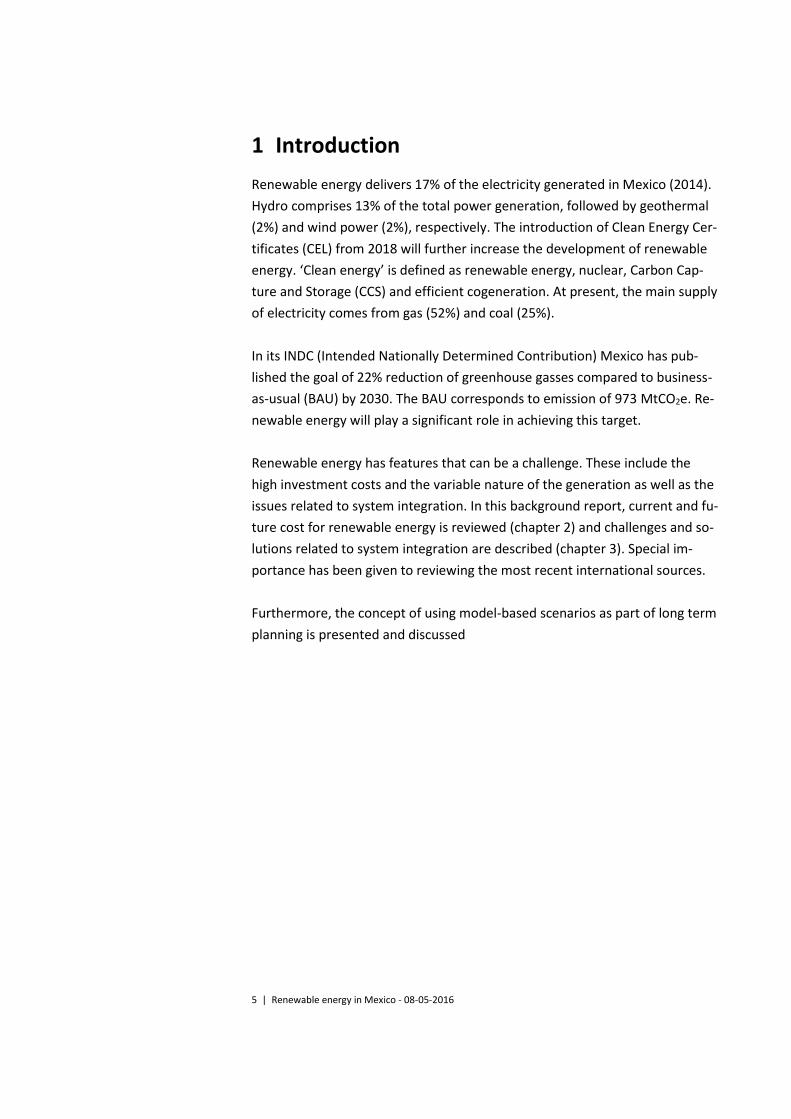
1 Introduction
Renewable energy delivers 17% of the electricity generated in Mexico (2014).
Hydro comprises 13% of the total power generation, followed by geothermal
(2%) and wind power (2%), respectively. The introduction of Clean Energy Cer-
tificates (CEL) from 2018 will further increase the development of renewable
energy. ‘Clean energy’ is defined as renewable energy, nuclear, Carbon Cap-
ture and Storage (CCS) and efficient cogeneration. At present, the main supply
of electricity comes from gas (52%) and coal (25%).
In its INDC (Intended Nationally Determined Contribution) Mexico has pub-
lished the goal of 22% reduction of greenhouse gasses compared to business-
as-usual (BAU) by 2030. The BAU corresponds to emission of 973 MtCO2e. Re-
newable energy will play a significant role in achieving this target.
Renewable energy has features that can be a challenge. These include the
high investment costs and the variable nature of the generation as well as the
issues related to system integration. In this background report, current and fu-
ture cost for renewable energy is reviewed (chapter 2) and challenges and so-
lutions related to system integration are described (chapter 3). Special im-
portance has been given to reviewing the most recent international sources.
Furthermore, the concept of using model-based scenarios as part of long term
planning is presented and discussed
6 | Renewable energy in Mexico - 08-05-2016
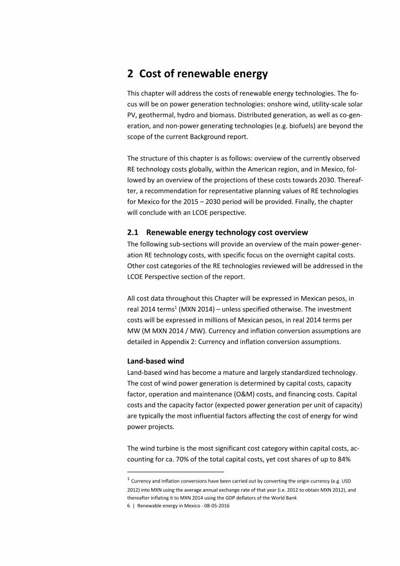
2 Cost of renewable energy
This chapter will address the costs of renewable energy technologies. The fo-
cus will be on power generation technologies: onshore wind, utility-scale solar
PV, geothermal, hydro and biomass. Distributed generation, as well as co-gen-
eration, and non-power generating technologies (e.g. biofuels) are beyond the
scope of the current Background report.
The structure of this chapter is as follows: overview of the currently observed
RE technology costs globally, within the American region, and in Mexico, fol-
lowed by an overview of the projections of these costs towards 2030. Thereaf-
ter, a recommendation for representative planning values of RE technologies
for Mexico for the 2015 – 2030 period will be provided. Finally, the chapter
will conclude with an LCOE perspective.
2.1 Renewable energy technology cost overview
The following sub-sections will provide an overview of the main power-gener-
ation RE technology costs, with specific focus on the overnight capital costs.
Other cost categories of the RE technologies reviewed will be addressed in the
LCOE Perspective section of the report.
All cost data throughout this Chapter will be expressed in Mexican pesos, in
real 2014 terms1 (MXN 2014) – unless specified otherwise. The investment
costs will be expressed in millions of Mexican pesos, in real 2014 terms per
MW (M MXN 2014 / MW). Currency and inflation conversion assumptions are
detailed in Appendix 2: Currency and inflation conversion assumptions.
Land-based wind
Land-based wind has become a mature and largely standardized technology.
The cost of wind power generation is determined by capital costs, capacity
factor, operation and maintenance (O&M) costs, and financing costs. Capital
costs and the capacity factor (expected power generation per unit of capacity)
are typically the most influential factors affecting the cost of energy for wind
power projects.
The wind turbine is the most significant cost category within capital costs, ac-
counting for ca. 70% of the total capital costs, yet cost shares of up to 84%
1 Currency and inflation conversions have been carried out by converting the origin currency (e.g. USD
2012) into MXN using the average annual exchange rate of that year (i.e. 2012 to obtain MXN 2012), and
thereafter inflating it to MXN 2014 using the GDP deflators of the World Bank
7 | Renewable energy in Mexico - 08-05-2016
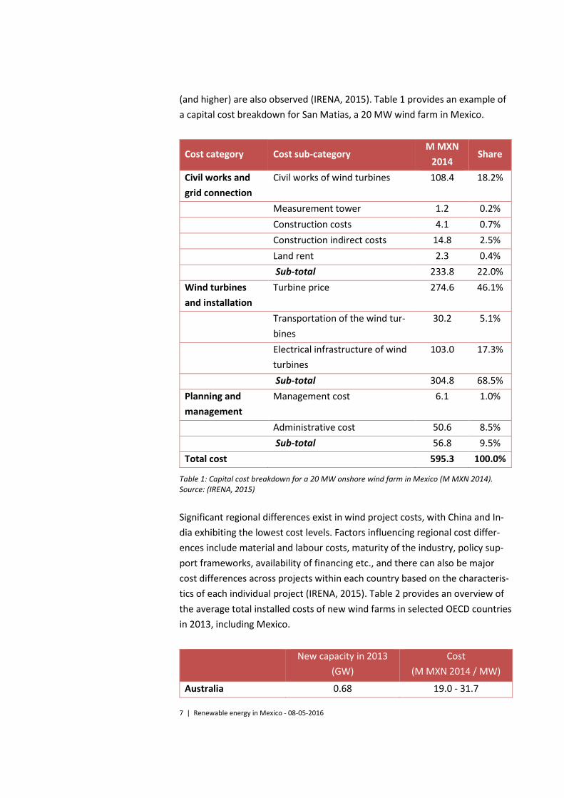
(and higher) are also observed (IRENA, 2015). Table 1 provides an example of
a capital cost breakdown for San Matias, a 20 MW wind farm in Mexico.
Cost category Cost sub-category M MXN
2014 Share
Civil works and
grid connection
Civil works of wind turbines 108.4 18.2%
Measurement tower 1.2 0.2%
Construction costs 4.1 0.7%
Construction indirect costs 14.8 2.5%
Land rent 2.3 0.4%
Sub-total 233.8 22.0%
Wind turbines
and installation
Turbine price 274.6 46.1%
Transportation of the wind tur-
bines
30.2 5.1%
Electrical infrastructure of wind
turbines
103.0 17.3%
Sub-total 304.8 68.5%
Planning and
management
Management cost 6.1 1.0%
Administrative cost 50.6 8.5%
Sub-total 56.8 9.5%
Total cost 595.3 100.0%
Table 1: Capital cost breakdown for a 20 MW onshore wind farm in Mexico (M MXN 2014). Source: (IRENA, 2015)
Significant regional differences exist in wind project costs, with China and In-
dia exhibiting the lowest cost levels. Factors influencing regional cost differ-
ences include material and labour costs, maturity of the industry, policy sup-
port frameworks, availability of financing etc., and there can also be major
cost differences across projects within each country based on the characteris-
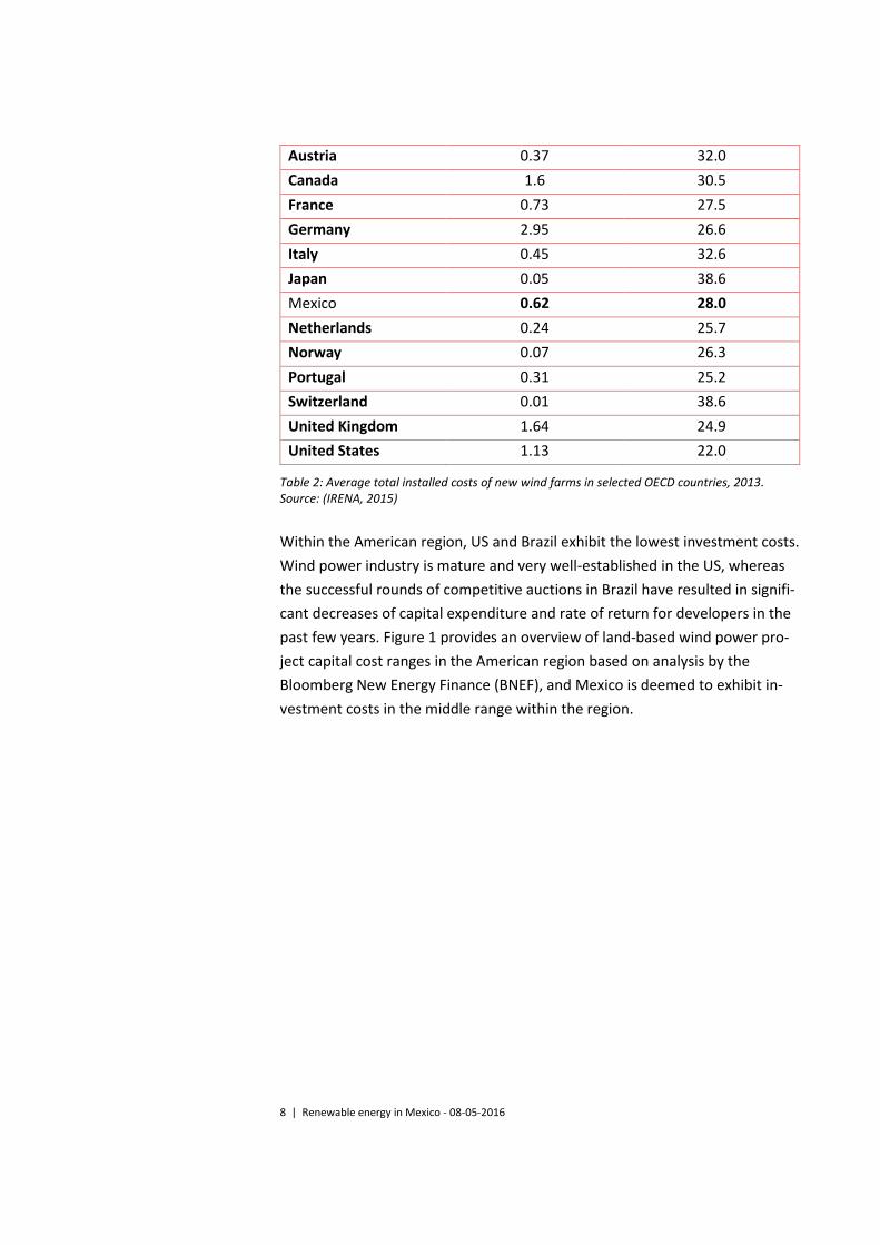
tics of each individual project (IRENA, 2015). Table 2 provides an overview of
the average total installed costs of new wind farms in selected OECD countries
in 2013, including Mexico.
New capacity in 2013
(GW)
Cost
(M MXN 2014 / MW)
Australia 0.68 19.0 - 31.7
8 | Renewable energy in Mexico - 08-05-2016
Austria 0.37 32.0
Canada 1.6 30.5
France 0.73 27.5
Germany 2.95 26.6
Italy 0.45 32.6
Japan 0.05 38.6
Mexico 0.62 28.0
Netherlands 0.24 25.7
Norway 0.07 26.3
Portugal 0.31 25.2
Switzerland 0.01 38.6
United Kingdom 1.64 24.9
United States 1.13 22.0
Table 2: Average total installed costs of new wind farms in selected OECD countries, 2013. Source: (IRENA, 2015)
Within the American region, US and Brazil exhibit the lowest investment costs.
Wind power industry is mature and very well-established in the US, whereas
the successful rounds of competitive auctions in Brazil have resulted in signifi-
cant decreases of capital expenditure and rate of return for developers in the
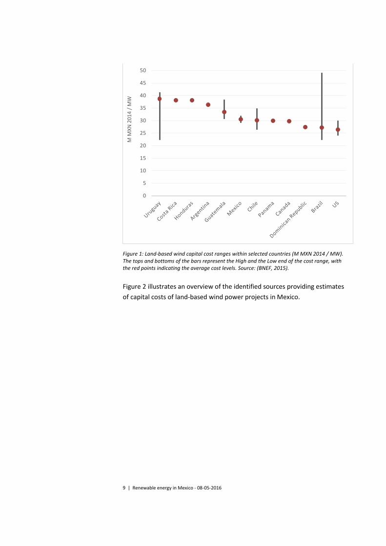
past few years. Figure 1 provides an overview of land-based wind power pro-
ject capital cost ranges in the American region based on analysis by the
Bloomberg New Energy Finance (BNEF), and Mexico is deemed to exhibit in-
vestment costs in the middle range within the region.
9 | Renewable energy in Mexico - 08-05-2016
Figure 1: Land-based wind capital cost ranges within selected countries (M MXN 2014 / MW). The tops and bottoms of the bars represent the High and the Low end of the cost range, with the red points indicating the average cost levels. Source: (BNEF, 2015).
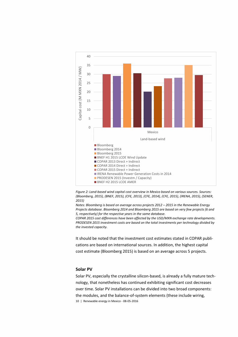
Figure 2 illustrates an overview of the identified sources providing estimates
of capital costs of land-based wind power projects in Mexico.
0
5
10
15
20
25
30
35
40
45
50
M M
XN
20
14
/ M
W
10 | Renewable energy in Mexico - 08-05-2016
Figure 2: Land-based wind capital cost overview in Mexico based on various sources. Sources: (Bloomberg, 2015), (BNEF, 2015), (CFE, 2013), (CFE, 2014), (CFE, 2015), (IRENA, 2015), (SENER, 2015) Notes: Bloomberg is based on average across projects 2012 – 2015 in the Renewable Energy Projects database. Bloomberg 2014 and Bloomberg 2015 are based on very few projects (6 and 5, respectively) for the respective years in the same database. COPAR 2015 cost differences have been affected by the USD/MXN exchange rate developments. PRODESEN 2015 investment costs are based on the total investments per technology divided by the invested capacity.
It should be noted that the investment cost estimates stated in COPAR publi-
cations are based on international sources. In addition, the highest capital
cost estimate (Bloomberg 2015) is based on an average across 5 projects.
Solar PV
Solar PV, especially the crystalline silicon-based, is already a fully mature tech-
nology, that nonetheless has continued exhibiting significant cost decreases
over time. Solar PV installations can be divided into two broad components:
the modules, and the balance-of-system elements (these include wiring,
0
5
10
15
20
25
30
35
40
Mexico
Land-based wind
Cap
ital
co
st (
M M
XN
20
14
/ M
W)
BloombergBloomberg 2014Bloomberg 2015BNEF H1 2015 LCOE Wind UpdateCOPAR 2013 Direct + IndirectCOPAR 2014 Direct + IndirectCOPAR 2015 Direct + IndirectIRENA Renewable Power Generation Costs in 2014PRODESEN 2015 (Investm / Capacity)BNEF H2 2015 LCOE AMER
11 | Renewable energy in Mexico - 08-05-2016
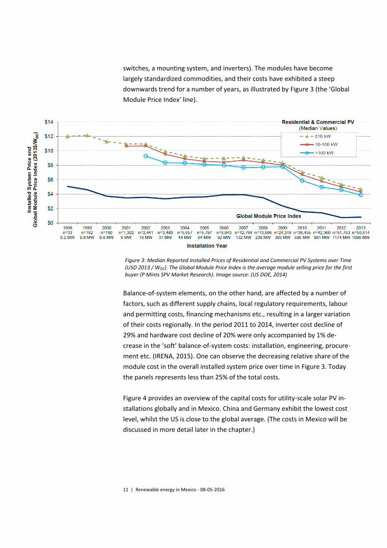
switches, a mounting system, and inverters). The modules have become
largely standardized commodities, and their costs have exhibited a steep
downwards trend for a number of years, as illustrated by Figure 3 (the ‘Global
Module Price Index’ line).
Figure 3: Median Reported Installed Prices of Residential and Commercial PV Systems over Time (USD 2013 / WDC). The Global Module Price Index is the average module selling price for the first buyer (P Mints SPV Market Research). Image source: (US DOE, 2014)
Balance-of-system elements, on the other hand, are affected by a number of
factors, such as different supply chains, local regulatory requirements, labour
and permitting costs, financing mechanisms etc., resulting in a larger variation
of their costs regionally. In the period 2011 to 2014, inverter cost decline of
29% and hardware cost decline of 20% were only accompanied by 1% de-
crease in the ‘soft’ balance-of-system costs: installation, engineering, procure-
ment etc. (IRENA, 2015). One can observe the decreasing relative share of the
module cost in the overall installed system price over time in Figure 3. Today
the panels represents less than 25% of the total costs.
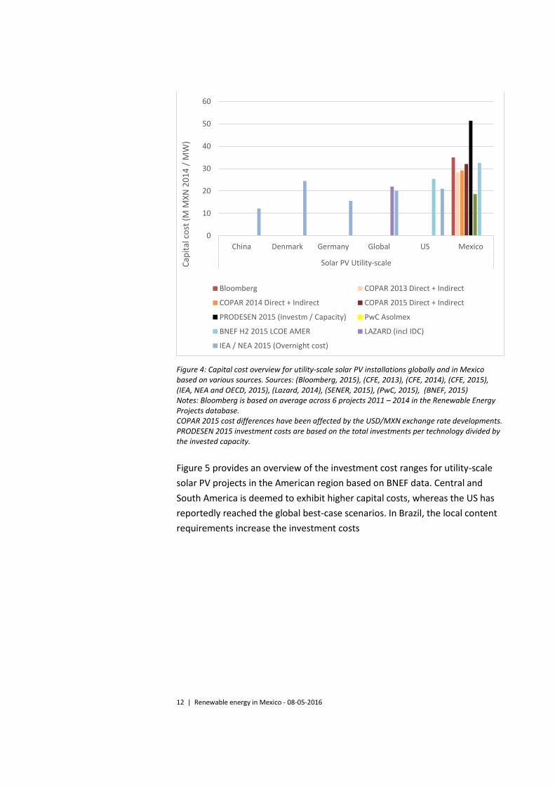
Figure 4 provides an overview of the capital costs for utility-scale solar PV in-
stallations globally and in Mexico. China and Germany exhibit the lowest cost
level, whilst the US is close to the global average. (The costs in Mexico will be
discussed in more detail later in the chapter.)
12 | Renewable energy in Mexico - 08-05-2016
Figure 4: Capital cost overview for utility-scale solar PV installations globally and in Mexico based on various sources. Sources: (Bloomberg, 2015), (CFE, 2013), (CFE, 2014), (CFE, 2015), (IEA, NEA and OECD, 2015), (Lazard, 2014), (SENER, 2015), (PwC, 2015), (BNEF, 2015) Notes: Bloomberg is based on average across 6 projects 2011 – 2014 in the Renewable Energy Projects database. COPAR 2015 cost differences have been affected by the USD/MXN exchange rate developments. PRODESEN 2015 investment costs are based on the total investments per technology divided by the invested capacity.
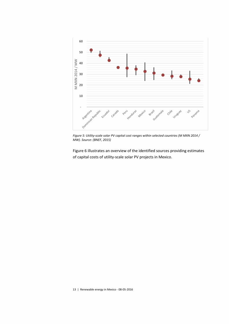
Figure 5 provides an overview of the investment cost ranges for utility-scale
solar PV projects in the American region based on BNEF data. Central and
South America is deemed to exhibit higher capital costs, whereas the US has
reportedly reached the global best-case scenarios. In Brazil, the local content
requirements increase the investment costs
0
10
20
30
40
50
60
China Denmark Germany Global US Mexico
Solar PV Utility-scaleCap
ital
co
st (
M M
XN
20
14
/ M
W)
Bloomberg COPAR 2013 Direct + Indirect
COPAR 2014 Direct + Indirect COPAR 2015 Direct + Indirect
PRODESEN 2015 (Investm / Capacity) PwC Asolmex
BNEF H2 2015 LCOE AMER LAZARD (incl IDC)
IEA / NEA 2015 (Overnight cost)
13 | Renewable energy in Mexico - 08-05-2016
Figure 5: Utility-scale solar PV capital cost ranges within selected countries (M MXN 2014 / MW). Source: (BNEF, 2015)
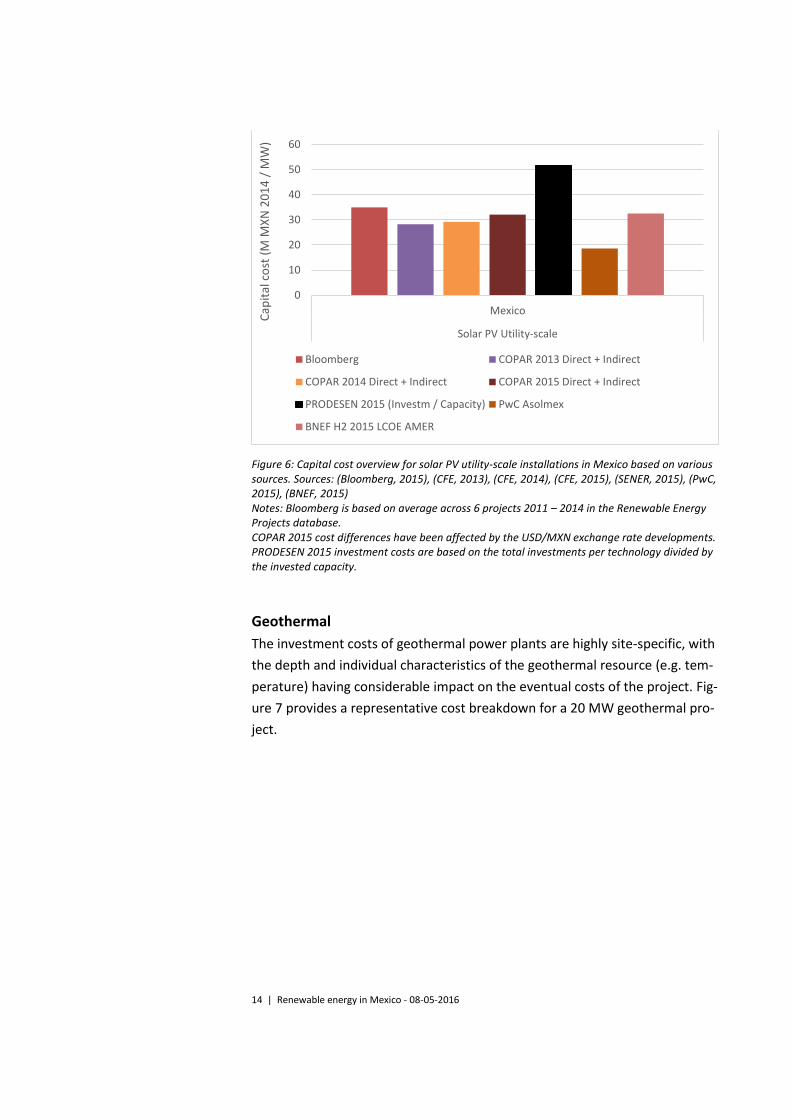
Figure 6 illustrates an overview of the identified sources providing estimates
of capital costs of utility-scale solar PV projects in Mexico.
-
10
20
30
40
50
60
M M
XN
20
14
/ M
W
14 | Renewable energy in Mexico - 08-05-2016
Figure 6: Capital cost overview for solar PV utility-scale installations in Mexico based on various sources. Sources: (Bloomberg, 2015), (CFE, 2013), (CFE, 2014), (CFE, 2015), (SENER, 2015), (PwC, 2015), (BNEF, 2015) Notes: Bloomberg is based on average across 6 projects 2011 – 2014 in the Renewable Energy Projects database. COPAR 2015 cost differences have been affected by the USD/MXN exchange rate developments. PRODESEN 2015 investment costs are based on the total investments per technology divided by the invested capacity.
Geothermal
The investment costs of geothermal power plants are highly site-specific, with
the depth and individual characteristics of the geothermal resource (e.g. tem-
perature) having considerable impact on the eventual costs of the project. Fig-
ure 7 provides a representative cost breakdown for a 20 MW geothermal pro-
ject.
0
10
20
30
40
50
60
Mexico
Solar PV Utility-scale
Cap
ital
co
st (
M M
XN
20
14
/ M
W)
Bloomberg COPAR 2013 Direct + Indirect
COPAR 2014 Direct + Indirect COPAR 2015 Direct + Indirect
PRODESEN 2015 (Investm / Capacity) PwC Asolmex
BNEF H2 2015 LCOE AMER
15 | Renewable energy in Mexico - 08-05-2016
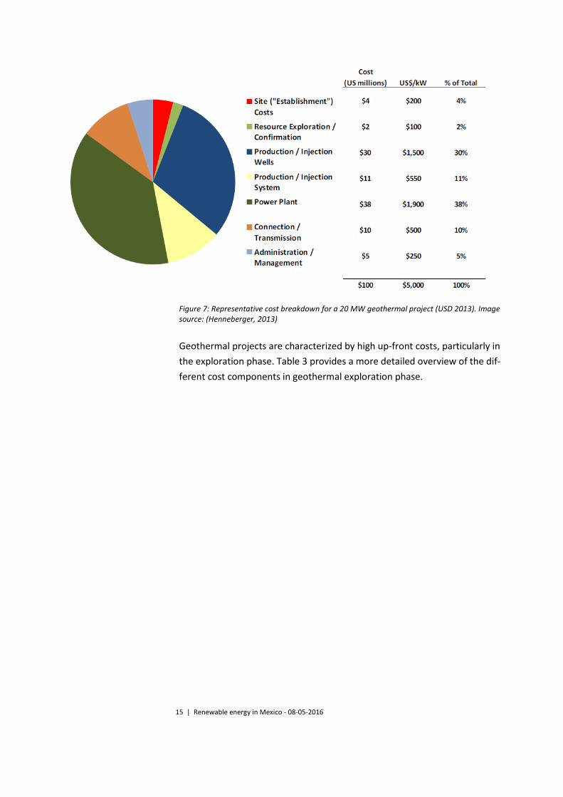
Figure 7: Representative cost breakdown for a 20 MW geothermal project (USD 2013). Image source: (Henneberger, 2013)
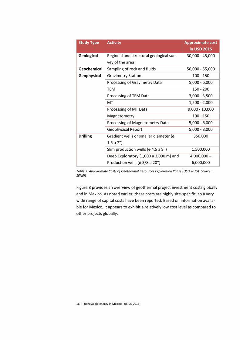
Geothermal projects are characterized by high up-front costs, particularly in
the exploration phase. Table 3 provides a more detailed overview of the dif-
ferent cost components in geothermal exploration phase.
16 | Renewable energy in Mexico - 08-05-2016
Study Type Activity Approximate cost
in USD 2015
Geological Regional and structural geological sur-
vey of the area
30,000 - 45,000
Geochemical Sampling of rock and fluids 50,000 - 55,000
Geophysical Gravimetry Station 100 - 150
Processing of Gravimetry Data 5,000 - 6,000
TEM 150 - 200
Processing of TEM Data 3,000 - 3,500
MT 1,500 - 2,000
Processing of MT Data 9,000 - 10,000
Magnetometry 100 - 150
Processing of Magnetometry Data 5,000 - 6,000
Geophysical Report 5,000 - 8,000
Drilling Gradient wells or smaller diameter (ø
1.5 a 7'')
350,000
Slim production wells (ø 4.5 a 9'') 1,500,000
Deep Exploratory (1,000 a 3,000 m) and
Production well, (ø 3/8 a 20'')
4,000,000 –
6,000,000
Table 3: Approximate Costs of Geothermal Resources Exploration Phase (USD 2015). Source: SENER
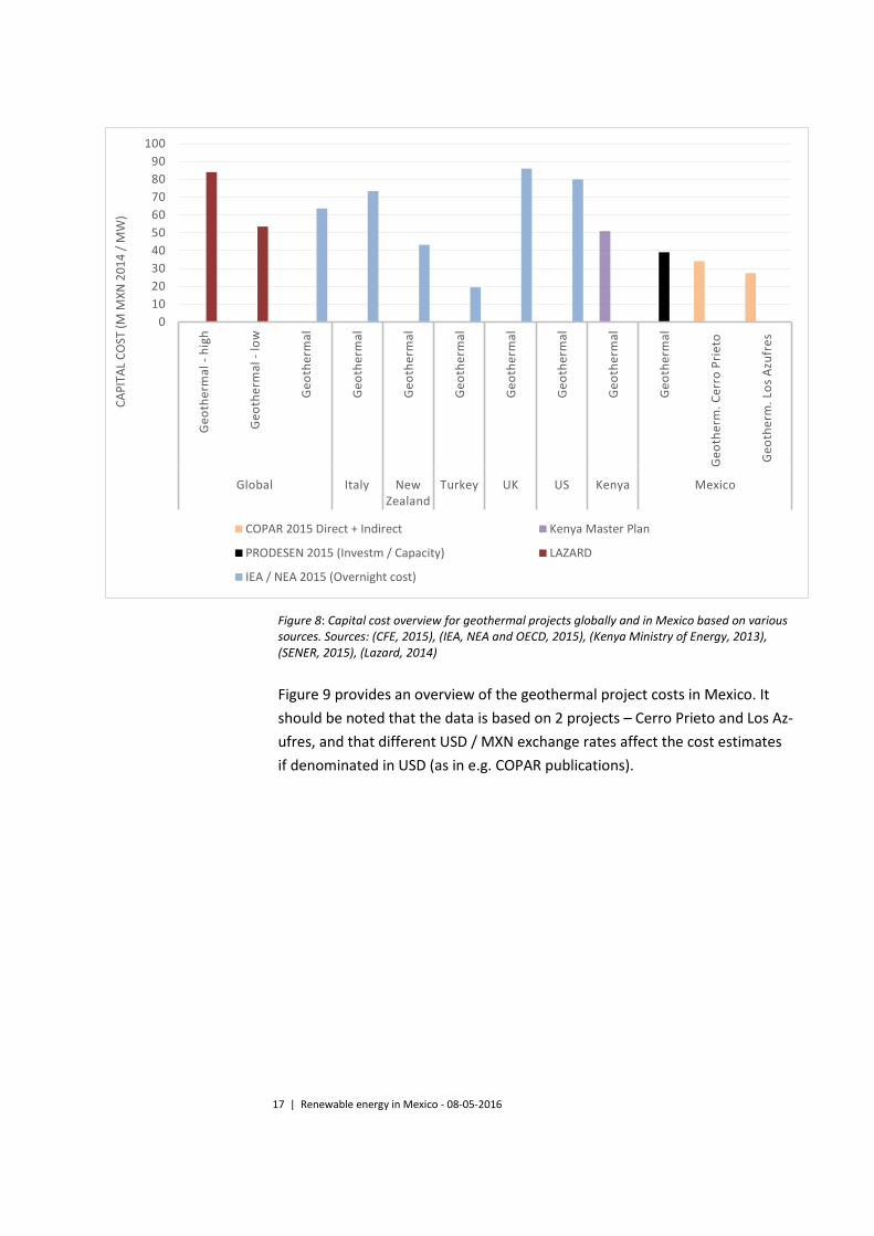
Figure 8 provides an overview of geothermal project investment costs globally
and in Mexico. As noted earlier, these costs are highly site-specific, so a very
wide range of capital costs have been reported. Based on information availa-
ble for Mexico, it appears to exhibit a relatively low cost level as compared to
other projects globally.
17 | Renewable energy in Mexico - 08-05-2016
Figure 8: Capital cost overview for geothermal projects globally and in Mexico based on various sources. Sources: (CFE, 2015), (IEA, NEA and OECD, 2015), (Kenya Ministry of Energy, 2013), (SENER, 2015), (Lazard, 2014)
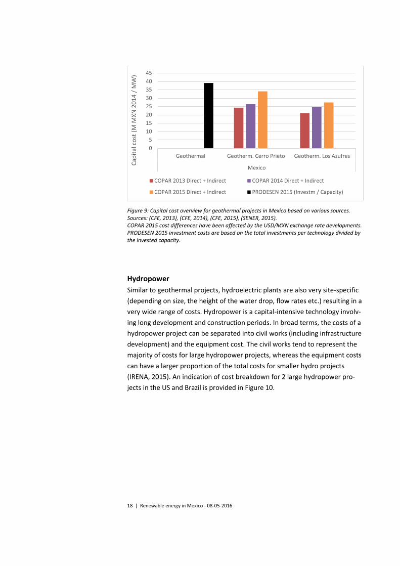
Figure 9 provides an overview of the geothermal project costs in Mexico. It
should be noted that the data is based on 2 projects – Cerro Prieto and Los Az-
ufres, and that different USD / MXN exchange rates affect the cost estimates
if denominated in USD (as in e.g. COPAR publications).
0
10
20
30
40
50
60
70
80
90
100
Ge
oth
erm
al -
hig
h
Ge
oth
erm
al -
low
Ge
oth
erm
al
Ge
oth
erm
al
Ge
oth
erm
al
Ge
oth
erm
al
Ge
oth
erm
al
Ge
oth
erm
al
Ge
oth
erm
al
Ge
oth
erm
al
Ge
oth
erm
. C
err
o P
rie
to
Ge
oth
erm
. Lo
s A
zufr
es
Global Italy New Zealand
Turkey UK US Kenya Mexico
CA
PIT
AL
CO
ST (
M M
XN
20
14
/ M
W)
COPAR 2015 Direct + Indirect Kenya Master Plan
PRODESEN 2015 (Investm / Capacity) LAZARD
IEA / NEA 2015 (Overnight cost)
18 | Renewable energy in Mexico - 08-05-2016
Figure 9: Capital cost overview for geothermal projects in Mexico based on various sources. Sources: (CFE, 2013), (CFE, 2014), (CFE, 2015), (SENER, 2015). COPAR 2015 cost differences have been affected by the USD/MXN exchange rate developments. PRODESEN 2015 investment costs are based on the total investments per technology divided by the invested capacity.
Hydropower
Similar to geothermal projects, hydroelectric plants are also very site-specific
(depending on size, the height of the water drop, flow rates etc.) resulting in a
very wide range of costs. Hydropower is a capital-intensive technology involv-
ing long development and construction periods. In broad terms, the costs of a
hydropower project can be separated into civil works (including infrastructure
development) and the equipment cost. The civil works tend to represent the
majority of costs for large hydropower projects, whereas the equipment costs
can have a larger proportion of the total costs for smaller hydro projects
(IRENA, 2015). An indication of cost breakdown for 2 large hydropower pro-
jects in the US and Brazil is provided in Figure 10.
0
5
10
15
20
25
30
35
40
45
Geothermal Geotherm. Cerro Prieto Geotherm. Los Azufres
Mexico
Cap
ital
co
st (
M M
XN
20
14
/ M
W)
COPAR 2013 Direct + Indirect COPAR 2014 Direct + Indirect
COPAR 2015 Direct + Indirect PRODESEN 2015 (Investm / Capacity)
19 | Renewable energy in Mexico - 08-05-2016
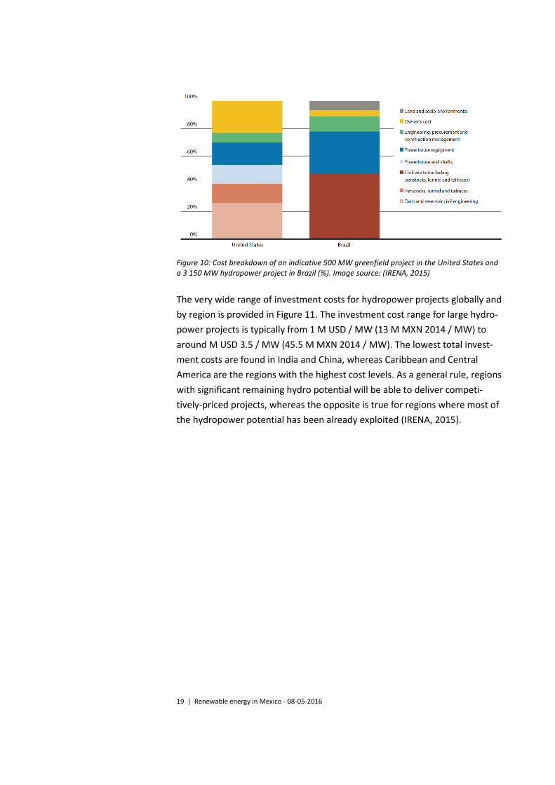
Figure 10: Cost breakdown of an indicative 500 MW greenfield project in the United States and a 3 150 MW hydropower project in Brazil (%). Image source: (IRENA, 2015)
The very wide range of investment costs for hydropower projects globally and
by region is provided in Figure 11. The investment cost range for large hydro-
power projects is typically from 1 M USD / MW (13 M MXN 2014 / MW) to
around M USD 3.5 / MW (45.5 M MXN 2014 / MW). The lowest total invest-
ment costs are found in India and China, whereas Caribbean and Central
America are the regions with the highest cost levels. As a general rule, regions
with significant remaining hydro potential will be able to deliver competi-
tively-priced projects, whereas the opposite is true for regions where most of
the hydropower potential has been already exploited (IRENA, 2015).
20 | Renewable energy in Mexico - 08-05-2016
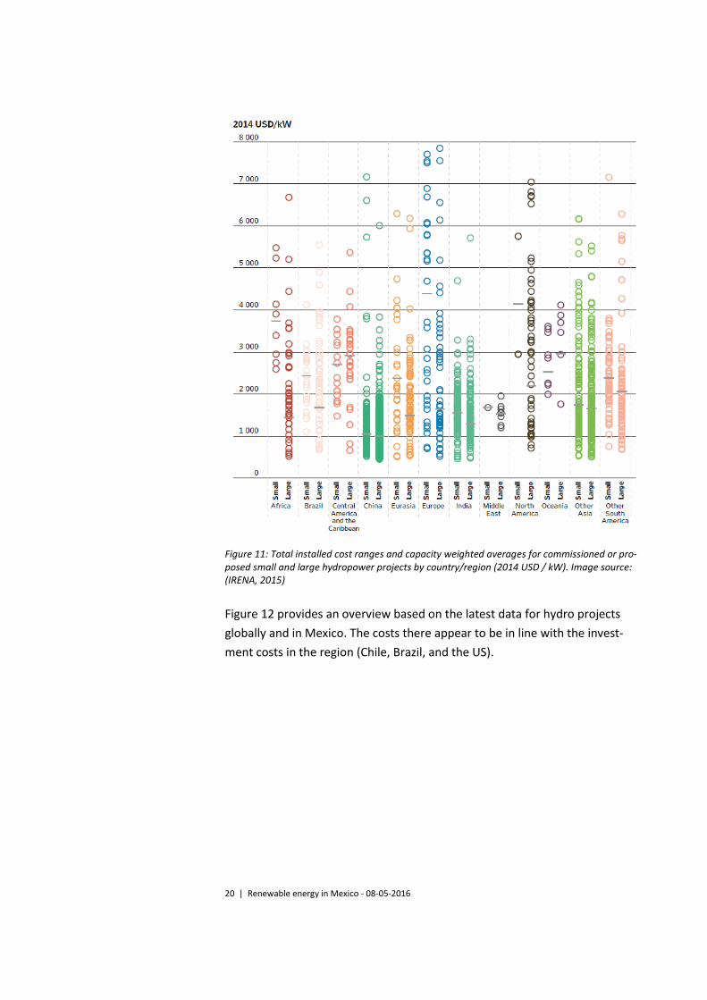
Figure 11: Total installed cost ranges and capacity weighted averages for commissioned or pro-posed small and large hydropower projects by country/region (2014 USD / kW). Image source: (IRENA, 2015)
Figure 12 provides an overview based on the latest data for hydro projects
globally and in Mexico. The costs there appear to be in line with the invest-
ment costs in the region (Chile, Brazil, and the US).
21 | Renewable energy in Mexico - 08-05-2016
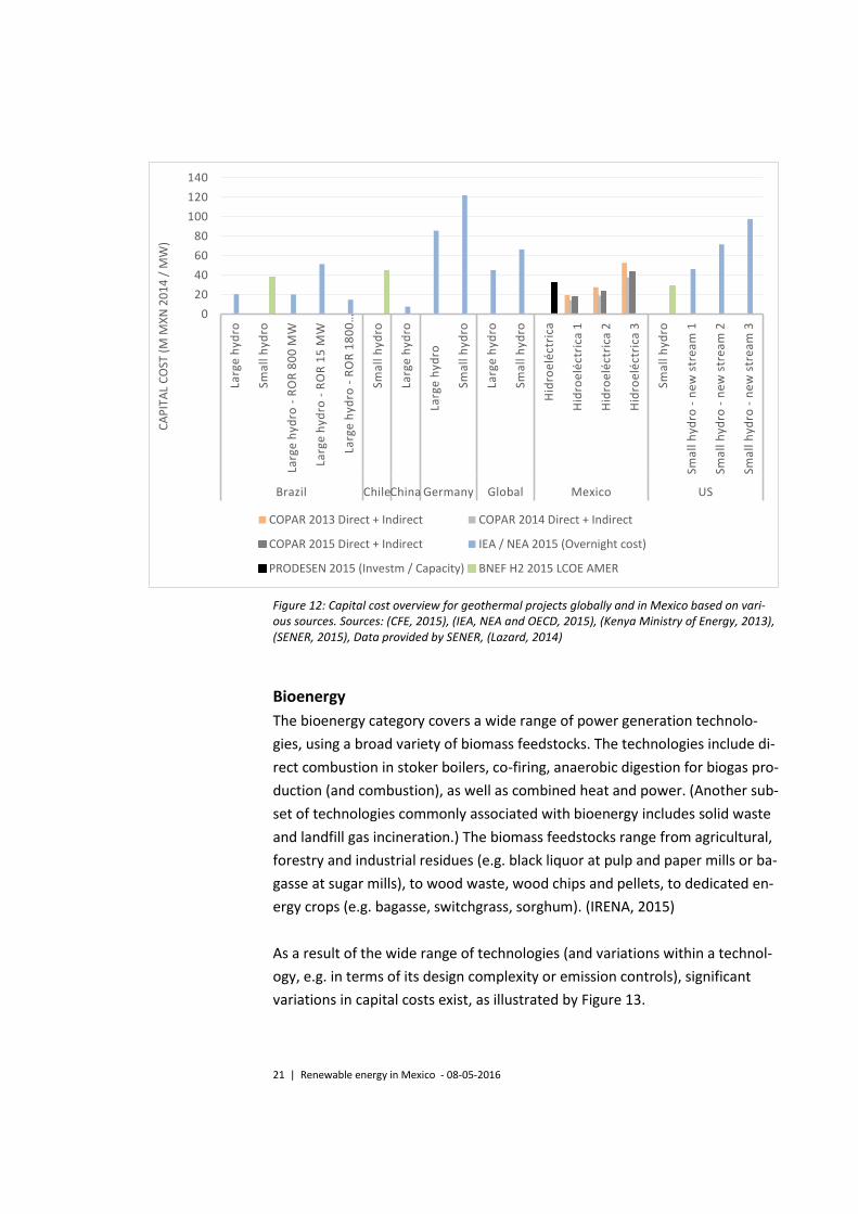
Figure 12: Capital cost overview for geothermal projects globally and in Mexico based on vari-ous sources. Sources: (CFE, 2015), (IEA, NEA and OECD, 2015), (Kenya Ministry of Energy, 2013), (SENER, 2015), Data provided by SENER, (Lazard, 2014)
Bioenergy
The bioenergy category covers a wide range of power generation technolo-
gies, using a broad variety of biomass feedstocks. The technologies include di-
rect combustion in stoker boilers, co-firing, anaerobic digestion for biogas pro-
duction (and combustion), as well as combined heat and power. (Another sub-
set of technologies commonly associated with bioenergy includes solid waste
and landfill gas incineration.) The biomass feedstocks range from agricultural,
forestry and industrial residues (e.g. black liquor at pulp and paper mills or ba-
gasse at sugar mills), to wood waste, wood chips and pellets, to dedicated en-
ergy crops (e.g. bagasse, switchgrass, sorghum). (IRENA, 2015)
As a result of the wide range of technologies (and variations within a technol-
ogy, e.g. in terms of its design complexity or emission controls), significant
variations in capital costs exist, as illustrated by Figure 13.
0
20
40
60
80
100
120
140
Larg
e h
ydro
Sma
ll h
ydro
Larg
e h
ydro
-R
OR
80
0 M
W
Larg
e h
ydro
-R
OR
15
MW
Larg
e h
ydro
-R
OR
18
00
…
Sma
ll h
ydro
Larg
e h
ydro
Larg
e h
ydro
Sma
ll h
ydro
Larg
e h
ydro
Sma
ll h
ydro
Hid
roe
léct
rica
Hid
roe
léct
rica
1
Hid
roe
léct
rica
2
Hid
roe
léct
rica
3
Sma
ll h
ydro
Sma
ll h
ydro
-n
ew
str
ea
m 1
Sma
ll h
ydro
-n
ew
str
ea
m 2
Sma
ll h
ydro
-n
ew
str
ea
m 3
Brazil ChileChina Germany Global Mexico US
CA
PIT
AL
CO
ST (
M M
XN
20
14
/ M
W)
COPAR 2013 Direct + Indirect COPAR 2014 Direct + Indirect
COPAR 2015 Direct + Indirect IEA / NEA 2015 (Overnight cost)
PRODESEN 2015 (Investm / Capacity) BNEF H2 2015 LCOE AMER
22 | Renewable energy in Mexico - 08-05-2016
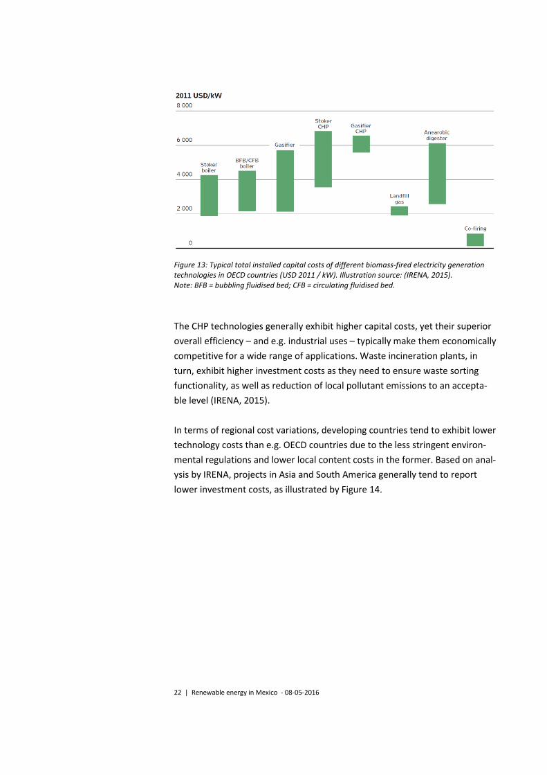
Figure 13: Typical total installed capital costs of different biomass-fired electricity generation technologies in OECD countries (USD 2011 / kW). Illustration source: (IRENA, 2015). Note: BFB = bubbling fluidised bed; CFB = circulating fluidised bed.
The CHP technologies generally exhibit higher capital costs, yet their superior
overall efficiency – and e.g. industrial uses – typically make them economically
competitive for a wide range of applications. Waste incineration plants, in
turn, exhibit higher investment costs as they need to ensure waste sorting
functionality, as well as reduction of local pollutant emissions to an accepta-
ble level (IRENA, 2015).
In terms of regional cost variations, developing countries tend to exhibit lower
technology costs than e.g. OECD countries due to the less stringent environ-
mental regulations and lower local content costs in the former. Based on anal-
ysis by IRENA, projects in Asia and South America generally tend to report
lower investment costs, as illustrated by Figure 14.
23 | Renewable energy in Mexico - 08-05-2016
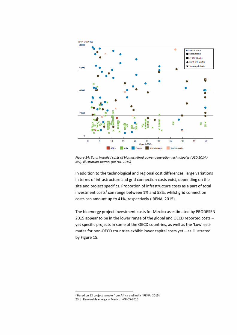
Figure 14: Total installed costs of biomass-fired power generation technologies (USD 2014 / kW). Illustration source: (IRENA, 2015)
In addition to the technological and regional cost differences, large variations
in terms of infrastructure and grid connection costs exist, depending on the
site and project specifics. Proportion of infrastructure costs as a part of total
investment costs2 can range between 1% and 58%, whilst grid connection
costs can amount up to 41%, respectively (IRENA, 2015).
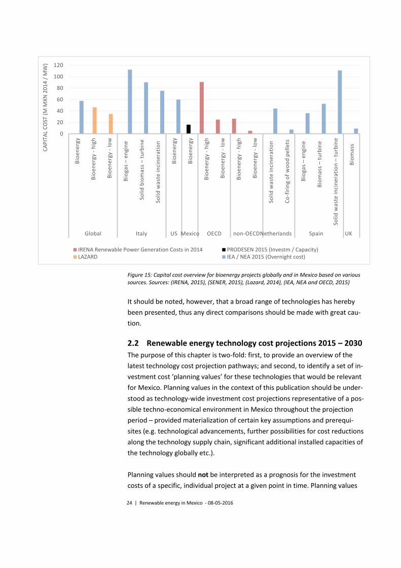
The bioenergy project investment costs for Mexico as estimated by PRODESEN
2015 appear to be in the lower range of the global and OECD reported costs –
yet specific projects in some of the OECD countries, as well as the ‘Low’ esti-
mates for non-OECD countries exhibit lower capital costs yet – as illustrated
by Figure 15.
2 Based on 12 project sample from Africa and India (IRENA, 2015)
24 | Renewable energy in Mexico - 08-05-2016
Figure 15: Capital cost overview for bioenergy projects globally and in Mexico based on various sources. Sources: (IRENA, 2015), (SENER, 2015), (Lazard, 2014), (IEA, NEA and OECD, 2015)
It should be noted, however, that a broad range of technologies has hereby
been presented, thus any direct comparisons should be made with great cau-
tion.
2.2 Renewable energy technology cost projections 2015 – 2030
The purpose of this chapter is two-fold: first, to provide an overview of the
latest technology cost projection pathways; and second, to identify a set of in-
vestment cost ‘planning values’ for these technologies that would be relevant
for Mexico. Planning values in the context of this publication should be under-
stood as technology-wide investment cost projections representative of a pos-
sible techno-economical environment in Mexico throughout the projection
period – provided materialization of certain key assumptions and prerequi-
sites (e.g. technological advancements, further possibilities for cost reductions
along the technology supply chain, significant additional installed capacities of
the technology globally etc.).
Planning values should not be interpreted as a prognosis for the investment
costs of a specific, individual project at a given point in time. Planning values
0
20
40
60
80
100
120
Bio
en
erg
y
Bio
en
erg
y -
hig
h
Bio
en
erg
y -
low
Bio
gas
–e
ngi
ne
Soli
d b
iom
ass
–tu
rbin
e
Soli
d w
ast
e in
cin
era
tio
n
Bio
en
erg
y
Bio
en
erg
y
Bio
en
erg
y -
hig
h
Bio
en
erg
y -
low
Bio
en
erg
y -
hig
h
Bio
en
erg
y -
low
Soli
d w
ast
e in
cin
era
tio
n
Co
-fir
ing
of
wo
od
pe
lle
ts
Bio
gas
–e
ngi
ne
Bio
ma
ss –
turb
ine
Soli
d w
ast
e in
cin
era
tio
n –
turb
ine
Bio
ma
ss
Global Italy US Mexico OECD non-OECDNetherlands Spain UK
CA
PIT
AL
CO
ST (
M M
XN
20
14
/ M
W)
IRENA Renewable Power Generation Costs in 2014 PRODESEN 2015 (Investm / Capacity)LAZARD IEA / NEA 2015 (Overnight cost)
25 | Renewable energy in Mexico - 08-05-2016
are neither necessarily direct extrapolation of the current costs and cost
trends observed in Mexico, as the present cost levels might be affected by
short-term factors (e.g. developer hesitation to progress projects due to up-
coming changes in the support policies, and higher costs due to lacking econo-
mies of scale in the industry as a result) as opposed to systematic, technology-
specific drivers.
Land-based wind
Land-based wind technology is deemed to be largely mature, and break-
through innovations are not considered the most likely sources of capital cost
reductions. Instead, evolutionary, incremental innovations (e.g. lower
drivetrain and nacelle costs, lower balance-of-plant and development costs
etc.) are expected to continue to reduce costs in the future. Figure 13 pro-
vides an overview of land-based wind capital cost projections. (It should be
noted, however, that some of the technological innovations – e.g. larger ro-
tors and higher towers – are associated with an additional capital expendi-
ture, whilst increasing annual energy production or allowing to utilize lower
wind speed sites and give higher full load hours. As such, the investment costs
are only one component in the wind power technology development path-
way, and should be regarded jointly with other key parameters within lev-
elized cost of energy (LCOE) framework – illustrated at the end of this chap-
ter.)
26 | Renewable energy in Mexico - 08-05-2016
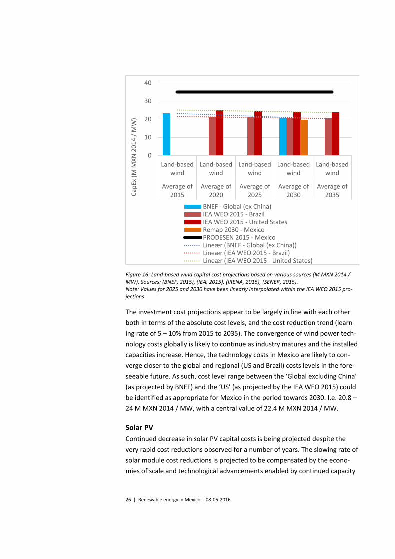
Figure 16: Land-based wind capital cost projections based on various sources (M MXN 2014 / MW). Sources: (BNEF, 2015), (IEA, 2015), (IRENA, 2015), (SENER, 2015). Note: Values for 2025 and 2030 have been linearly interpolated within the IEA WEO 2015 pro-jections
The investment cost projections appear to be largely in line with each other
both in terms of the absolute cost levels, and the cost reduction trend (learn-
ing rate of 5 – 10% from 2015 to 2035). The convergence of wind power tech-
nology costs globally is likely to continue as industry matures and the installed
capacities increase. Hence, the technology costs in Mexico are likely to con-
verge closer to the global and regional (US and Brazil) costs levels in the fore-
seeable future. As such, cost level range between the ‘Global excluding China’
(as projected by BNEF) and the ‘US’ (as projected by the IEA WEO 2015) could
be identified as appropriate for Mexico in the period towards 2030. I.e. 20.8 –
24 M MXN 2014 / MW, with a central value of 22.4 M MXN 2014 / MW.
Solar PV
Continued decrease in solar PV capital costs is being projected despite the
very rapid cost reductions observed for a number of years. The slowing rate of
solar module cost reductions is projected to be compensated by the econo-
mies of scale and technological advancements enabled by continued capacity
0
10
20
30
40
Land-basedwind
Land-basedwind
Land-basedwind
Land-basedwind
Land-basedwind
Average of2015
Average of2020
Average of2025
Average of2030
Average of2035C
apEx
(M
MX
N 2
01
4 /
MW
)
BNEF - Global (ex China)IEA WEO 2015 - BrazilIEA WEO 2015 - United StatesRemap 2030 - MexicoPRODESEN 2015 - MexicoLineær (BNEF - Global (ex China))Lineær (IEA WEO 2015 - Brazil)Lineær (IEA WEO 2015 - United States)
27 | Renewable energy in Mexico - 08-05-2016
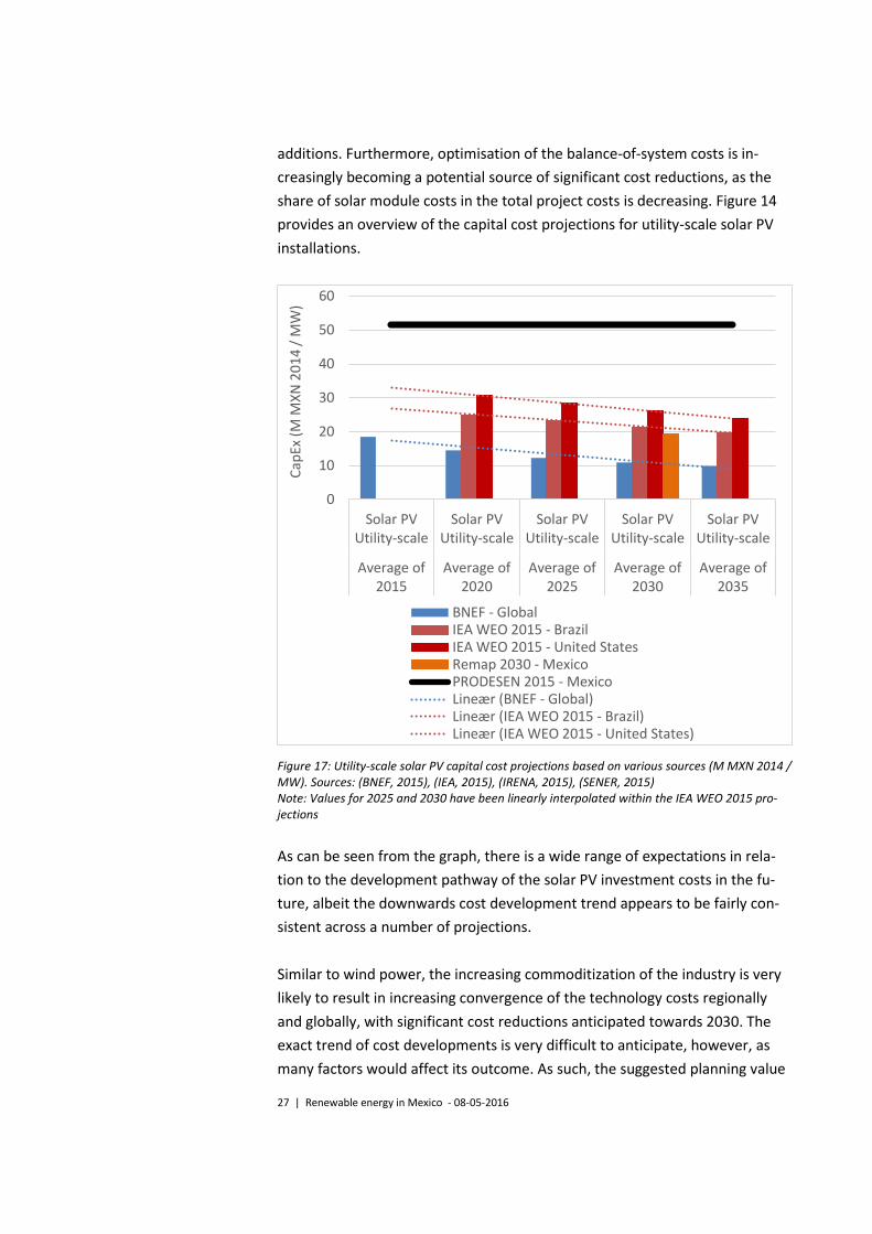
additions. Furthermore, optimisation of the balance-of-system costs is in-
creasingly becoming a potential source of significant cost reductions, as the
share of solar module costs in the total project costs is decreasing. Figure 14
provides an overview of the capital cost projections for utility-scale solar PV
installations.
Figure 17: Utility-scale solar PV capital cost projections based on various sources (M MXN 2014 / MW). Sources: (BNEF, 2015), (IEA, 2015), (IRENA, 2015), (SENER, 2015) Note: Values for 2025 and 2030 have been linearly interpolated within the IEA WEO 2015 pro-jections
As can be seen from the graph, there is a wide range of expectations in rela-
tion to the development pathway of the solar PV investment costs in the fu-
ture, albeit the downwards cost development trend appears to be fairly con-
sistent across a number of projections.
Similar to wind power, the increasing commoditization of the industry is very
likely to result in increasing convergence of the technology costs regionally
and globally, with significant cost reductions anticipated towards 2030. The
exact trend of cost developments is very difficult to anticipate, however, as
many factors would affect its outcome. As such, the suggested planning value
0
10
20
30
40
50
60
Solar PVUtility-scale
Solar PVUtility-scale
Solar PVUtility-scale
Solar PVUtility-scale
Solar PVUtility-scale
Average of2015
Average of2020
Average of2025
Average of2030
Average of2035
Cap
Ex (
M M
XN
20
14
/ M
W)
BNEF - GlobalIEA WEO 2015 - BrazilIEA WEO 2015 - United StatesRemap 2030 - MexicoPRODESEN 2015 - MexicoLineær (BNEF - Global)Lineær (IEA WEO 2015 - Brazil)Lineær (IEA WEO 2015 - United States)
28 | Renewable energy in Mexico - 08-05-2016
range for utility-scale solar PV installations for 2030 would be between the
ambitious ‘Global’ (BNEF) and the more moderate ‘Brazil’ (IEA WEO 2015) es-
timate, i.e. 10.9 – 21.4 M MXN 2014 / MW, with a central value of 16.2 M
MXN 2014 / MW.
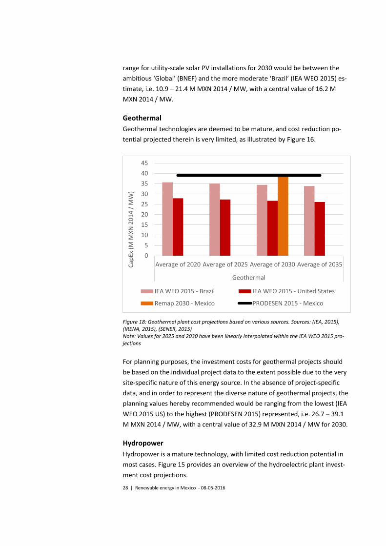
Geothermal
Geothermal technologies are deemed to be mature, and cost reduction po-
tential projected therein is very limited, as illustrated by Figure 16.
Figure 18: Geothermal plant cost projections based on various sources. Sources: (IEA, 2015), (IRENA, 2015), (SENER, 2015) Note: Values for 2025 and 2030 have been linearly interpolated within the IEA WEO 2015 pro-jections
For planning purposes, the investment costs for geothermal projects should
be based on the individual project data to the extent possible due to the very
site-specific nature of this energy source. In the absence of project-specific
data, and in order to represent the diverse nature of geothermal projects, the
planning values hereby recommended would be ranging from the lowest (IEA
WEO 2015 US) to the highest (PRODESEN 2015) represented, i.e. 26.7 – 39.1
M MXN 2014 / MW, with a central value of 32.9 M MXN 2014 / MW for 2030.
Hydropower
Hydropower is a mature technology, with limited cost reduction potential in
most cases. Figure 15 provides an overview of the hydroelectric plant invest-
ment cost projections.
0
5
10
15
20
25
30
35
40
45
Average of 2020 Average of 2025 Average of 2030 Average of 2035
Geothermal
Cap
Ex (
M M
XN
20
14
/ M
W)
IEA WEO 2015 - Brazil IEA WEO 2015 - United States
Remap 2030 - Mexico PRODESEN 2015 - Mexico
29 | Renewable energy in Mexico - 08-05-2016
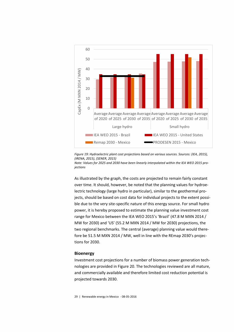
Figure 19: Hydroelectric plant cost projections based on various sources. Sources: (IEA, 2015), (IRENA, 2015), (SENER, 2015) Note: Values for 2025 and 2030 have been linearly interpolated within the IEA WEO 2015 pro-jections
As illustrated by the graph, the costs are projected to remain fairly constant
over time. It should, however, be noted that the planning values for hydroe-
lectric technology (large hydro in particular), similar to the geothermal pro-
jects, should be based on cost data for individual projects to the extent possi-
ble due to the very site-specific nature of this energy source. For small hydro
power, it is hereby proposed to estimate the planning value investment cost
range for Mexico between the IEA WEO 2015’s ‘Brazil’ (47.8 M MXN 2014 /
MW for 2030) and ‘US’ (55.2 M MXN 2014 / MW for 2030) projections, the
two regional benchmarks. The central (average) planning value would there-
fore be 51.5 M MXN 2014 / MW, well in line with the REmap 2030’s projec-
tions for 2030.
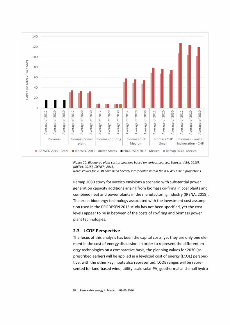
Bioenergy
Investment cost projections for a number of biomass power generation tech-
nologies are provided in Figure 20. The technologies reviewed are all mature,
and commercially available and therefore limited cost reduction potential is
projected towards 2030.
0
10
20
30
40
50
60
Averageof 2020
Averageof 2025
Averageof 2030
Averageof 2035
Averageof 2020
Averageof 2025
Averageof 2030
Averageof 2035
Large hydro Small hydro
Cap
Ex (
M M
XN
20
14
/ M
W)
IEA WEO 2015 - Brazil IEA WEO 2015 - United States
Remap 2030 - Mexico PRODESEN 2015 - Mexico
30 | Renewable energy in Mexico - 08-05-2016
Figure 20: Bioenergy plant cost projections based on various sources. Sources: (IEA, 2015), (IRENA, 2015), (SENER, 2015) Note: Values for 2030 have been linearly interpolated within the IEA WEO 2015 projections
Remap 2030 study for Mexico envisions a scenario with substantial power
generation capacity additions arising from biomass co-firing in coal plants and
combined heat and power plants in the manufacturing industry (IRENA, 2015).
The exact bioenergy technology associated with the investment cost assump-
tion used in the PRODESEN 2015 study has not been specified, yet the cost
levels appear to be in between of the costs of co-firing and biomass power
plant technologies.
2.3 LCOE Perspective
The focus of this analysis has been the capital costs, yet they are only one ele-
ment in the cost of energy discussion. In order to represent the different en-
ergy technologies on a comparative basis, the planning values for 2030 (as
prescribed earlier) will be applied in a levelized cost of energy (LCOE) perspec-
tive, with the other key inputs also represented. LCOE ranges will be repre-
sented for land-based wind, utility-scale solar PV, geothermal and small hydro
0
20
40
60
80
100
120
140
Ave
rage
of
20
12
Ave
rage
of
20
20
Ave
rage
of
20
30
Ave
rage
of
20
12
Ave
rage
of
20
20
Ave
rage
of
20
30
Ave
rage
of
20
12
Ave
rage
of
20
20
Ave
rage
of
20
30
Ave
rage
of
20
12
Ave
rage
of
20
20
Ave
rage
of
20
30
Ave
rage
of
20
12
Ave
rage
of
20
20
Ave
rage
of
20
30
Ave
rage
of
20
12
Ave
rage
of
20
20
Ave
rage
of
20
30
Biomass Biomass power plant
Biomass Cofiring Biomass CHP Medium
Biomass CHP Small
Biomass - waste incineration - CHP
CA
PEX
(M
MX
N 2
01
4 /
MW
)
IEA WEO 2015 - Brazil IEA WEO 2015 - United States PRODESEN 2015 - Mexico Remap 2030 - Mexico
31 | Renewable energy in Mexico - 08-05-2016
technologies1. A spreadsheet-based cash flow model developed by the Energy
Research Centre of the Netherlands (ECN) has been applied for the LCOE cal-
culations, also used in the IEA Wind Task 26 – Cost of Wind Energy (IEA, 2015).
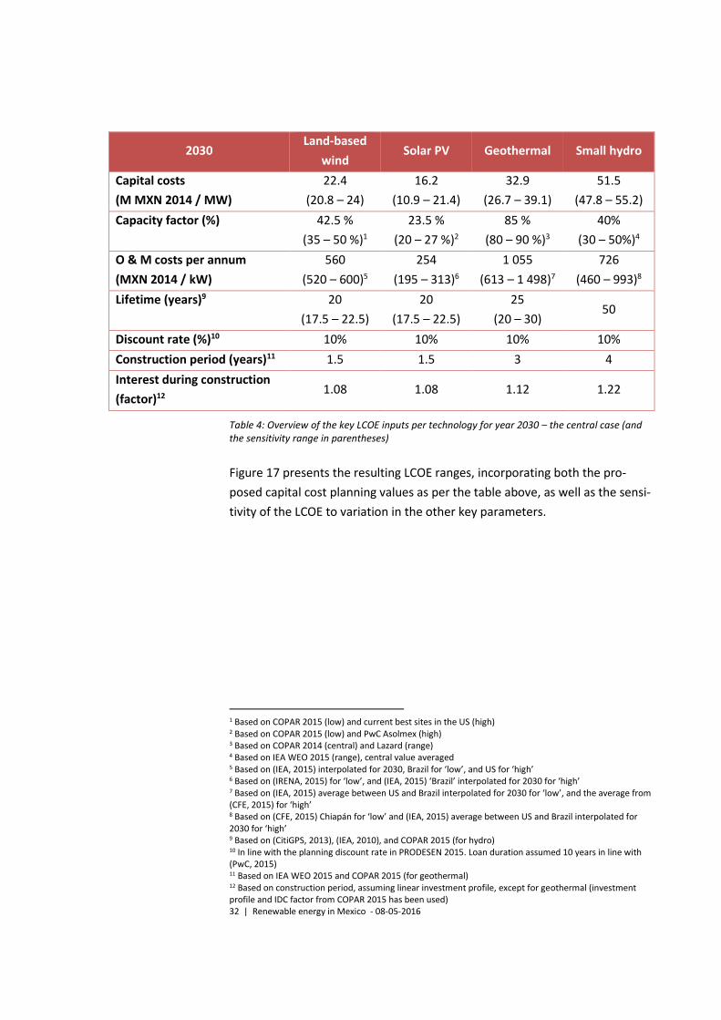
Table 4 provides an overview of the LCOE assumptions used in the calcula-
tions, representing the central (and the ranges) of the planning values used to
arrive at LCOE ranges for Mexico for 2030.
Additional assumptions include:
- Corporate tax rate of 30%
- Straight-line depreciation over 20-year period
- Loan duration of 10 years2
- Planning discount rate of 10%, in line with SENER methodology3 (i.e.
no representation of specific debt / equity financing structures and
rates)
- No subsidies or support schemes
- Calculation made in real terms, i.e. no inflation has been applied
- No decommissioning costs
- No efficiency loss incorporated for solar PV
1 LCOE ranges will not be estimated for large hydro, as these projects are too site-specific, and many other (e.g. environmental and social) factors need to be considered for a meaningful analysis. Biomass-fired tech-nologies will neither be considered as the diversity of technologies, applications and fuels (and costs thereof) would require a more in-depth analysis, which is beyond the scope of the current Background Re-port. 2 In line with (PwC, 2015) 3 In line with (SENER, 2015)
32 | Renewable energy in Mexico - 08-05-2016
2030 Land-based
wind Solar PV Geothermal Small hydro
Capital costs
(M MXN 2014 / MW)
22.4
(20.8 – 24)
16.2
(10.9 – 21.4)
32.9
(26.7 – 39.1)
51.5
(47.8 – 55.2)
Capacity factor (%) 42.5 %
(35 – 50 %)1
23.5 %
(20 – 27 %)2
85 %
(80 – 90 %)3
40%
(30 – 50%)4
O & M costs per annum
(MXN 2014 / kW)
560
(520 – 600)5
254
(195 – 313)6
1 055
(613 – 1 498)7
726
(460 – 993)8
Lifetime (years)9 20
(17.5 – 22.5)
20
(17.5 – 22.5)
25
(20 – 30) 50
Discount rate (%)10 10% 10% 10% 10%
Construction period (years)11 1.5 1.5 3 4
Interest during construction
(factor)12 1.08 1.08 1.12 1.22
Table 4: Overview of the key LCOE inputs per technology for year 2030 – the central case (and the sensitivity range in parentheses)
Figure 17 presents the resulting LCOE ranges, incorporating both the pro-
posed capital cost planning values as per the table above, as well as the sensi-
tivity of the LCOE to variation in the other key parameters.
1 Based on COPAR 2015 (low) and current best sites in the US (high) 2 Based on COPAR 2015 (low) and PwC Asolmex (high) 3 Based on COPAR 2014 (central) and Lazard (range) 4 Based on IEA WEO 2015 (range), central value averaged 5 Based on (IEA, 2015) interpolated for 2030, Brazil for ‘low’, and US for ‘high’ 6 Based on (IRENA, 2015) for ‘low’, and (IEA, 2015) ‘Brazil’ interpolated for 2030 for ‘high’ 7 Based on (IEA, 2015) average between US and Brazil interpolated for 2030 for ‘low’, and the average from (CFE, 2015) for ‘high’ 8 Based on (CFE, 2015) Chiapán for ‘low’ and (IEA, 2015) average between US and Brazil interpolated for 2030 for ‘high’ 9 Based on (CitiGPS, 2013), (IEA, 2010), and COPAR 2015 (for hydro) 10 In line with the planning discount rate in PRODESEN 2015. Loan duration assumed 10 years in line with (PwC, 2015) 11 Based on IEA WEO 2015 and COPAR 2015 (for geothermal) 12 Based on construction period, assuming linear investment profile, except for geothermal (investment profile and IDC factor from COPAR 2015 has been used)
33 | Renewable energy in Mexico - 08-05-2016
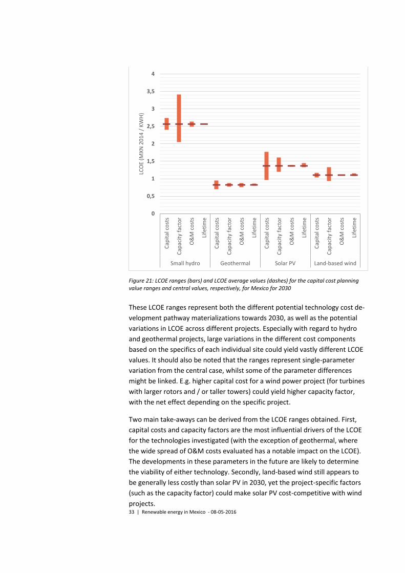
Figure 21: LCOE ranges (bars) and LCOE average values (dashes) for the capital cost planning value ranges and central values, respectively, for Mexico for 2030
These LCOE ranges represent both the different potential technology cost de-
velopment pathway materializations towards 2030, as well as the potential
variations in LCOE across different projects. Especially with regard to hydro
and geothermal projects, large variations in the different cost components
based on the specifics of each individual site could yield vastly different LCOE
values. It should also be noted that the ranges represent single-parameter
variation from the central case, whilst some of the parameter differences
might be linked. E.g. higher capital cost for a wind power project (for turbines
with larger rotors and / or taller towers) could yield higher capacity factor,
with the net effect depending on the specific project.
Two main take-aways can be derived from the LCOE ranges obtained. First,
capital costs and capacity factors are the most influential drivers of the LCOE
for the technologies investigated (with the exception of geothermal, where
the wide spread of O&M costs evaluated has a notable impact on the LCOE).
The developments in these parameters in the future are likely to determine
the viability of either technology. Secondly, land-based wind still appears to
be generally less costly than solar PV in 2030, yet the project-specific factors
(such as the capacity factor) could make solar PV cost-competitive with wind
projects.
0
0,5
1
1,5
2
2,5
3
3,5
4
Cap
ital
co
sts
Cap
acit
y fa
cto
r
O&
M c
ost
s
Life
tim
e
Cap
ital
co
sts
Cap
acit
y fa
cto
r
O&
M c
ost
s
Life
tim
e
Cap
ital
co
sts
Cap
acit
y fa
cto
r
O&
M c
ost
s
Life
tim
e
Cap
ital
co
sts
Cap
acit
y fa
cto
r
O&
M c
ost
s
Life
tim
e
Small hydro Geothermal Solar PV Land-based wind
LCO
E (M
XN
20
14
/ K
WH
)
34 | Renewable energy in Mexico - 08-05-2016
2.4 Implications for power system planning in Mexico
Accurate representation of technology characteristics and costs is of utmost
importance for objective and trustworthy power system development plan-
ning studies. Inconsistencies in the inputs, especially in least-cost planning
studies, lead to direct implications in the results, in terms of e.g. sub-optimal
generation fleet composition or investment timeline. This is especially true for
renewable energy sources (e.g. wind and solar PV) that, whilst being relatively
mature technologies, still exhibit significant cost reductions (and performance
improvements) that are projected to persist in the future.
The main focus of the current report has been renewable energy investment
costs. Investment costs (as illustrated by the LCOE analysis) are one of the key
determinants of the eventual cost of energy of a given technology, hence in-
consistencies in the assumptions thereof can lead to significantly altered out-
comes compared to an optimal least-cost power system development path-
way.
Capacity factors are another crucial characteristic of wind and solar technolo-
gies, and, albeit they have not been a key focus area of the current report, a
thorough review of the assumptions used in power system development plan-
ning could be recommended in order to accurately represent the potential of
renewable energy in the future in Mexico.
The planning values (planning value ranges) brought forward by the current
analysis could be either directly applied in the upcoming PRODESEN studies,
or used as input for alternative. This would help provide a more accurate and
nuanced representation of the latest developments of the renewable energy
technology costs (and projections thereof), and their prospective impact on
the optimal least-cost composition of the power system in Mexico in the fu-
ture.
35 | Renewable energy in Mexico - 08-05-2016
References to Chapter 2
Bloomberg. (2015). H1 2015 Wind LCOE Outlook. Bloomberg New Energy
Finance.
Bloomberg. (2015). New Energy Outlook 2015 - Americas. Bloomberg Finance
L.P.
Bloomberg. (2015). Renewable Energy Projects database. Bloomberg L.P.
BNEF. (2015). H1 2015 LCOE Wind Update. Bloomberg Finance L.P.
BNEF. (2015). H2 2015 Americas LCOE Outlook. Bloomberg L.P.
BNEF. (2015). New Energy Outlook 2015: Long-term projectionsof the global
energy sector. Solar June 2015. Bloomberg Finance L.P.
BNEF. (2015). The future cost of onshore wind – an accelerating rate of
progress . Bloomberg Finance L.P.
CFE. (2013). COPAR 2013. Mexico: Comisión Federal de Electricidad.
CFE. (2014). COPAR 2014. Mexico: Comisión Federal de Electricidad.
CFE. (2015). COPAR 2015. Mexico: Comisión Federal de Electricidad.
CitiGPS. (2013). ENERGY DARWINISM: The Evolution of the Energy Industry.
Citigroup.
Henneberger, R. (2013). Costs and Financial Risks of Geothermal Projects.
International Finance Corporation. Retrieved from
http://www.geothermal-energy.org/ifc-
iga_launch_event_best_practice_guide.html?no_cache=1&cid=694&d
id=144&sechash=9c6ff36f
IEA. (2010). Renewable Energy Essentials: Geothermal. Paris: OECD /
International Energy Agency.
IEA. (2015). IEA Wind Task 26 - Wind Technology, Cost, and Performance
Trends in Denmark, Germany, Ireland, Norway, the European Union,
and the United States: 2007–2012. Golden, CO: NREL.
IEA. (2015). World Energy Outlook 2015. Paris: International Energy Agency.
IEA, NEA and OECD. (2015). Projected Costs of Generating Electricity - 2015
Edition. Paris: OECD PUBLICATIONS.
IRENA. (2015). REmap 2030 Renewable Energy Prospects: Mexico. Abu Dhabi:
IRENA.
IRENA. (2015). Renewable Power Generation Costs in 2014. IRENA.
Kenya Ministry of Energy. (2013). Least Cost Power Development Plan 2013 -
2033. Nairobi: Kenya Ministry of Energy.
Lazard. (2014). Lazard's Levelized Cost of Energy Analysis - version 8.0. Lazard.
PwC. (2015). Estudio sobre las inversiones necesarias para que México cumpla
con sus metas de Energías Limpias. Mexico: PwC.
PwC. (2015). Iniciativa Solar Reunión de arranque - DOCUMENTO PARA
DISCUSIÓN Septiembre 2015. PwC.

36 | Renewable energy in Mexico - 08-05-2016
SENER. (2015). PRODESEN 2015 - 2029. Mexico: SENER.
US DOE. (2014). Photovoltaic System Pricing Trends - Historical, Recent, and
Near-Term Projections: 2014 Edition. SunShot U.S. Department of
Energy.
37 | Renewable energy in Mexico - 08-05-2016
3 System integration of renewable energy
The nature of the electricity system is such that the balance between demand
and supply must be maintained second by second. The intermittent genera-
tion from renewable energy sources, like wind and solar, is driven by the me-
teorological conditions and must continuously be balanced by other genera-
tion.
Successful integration of wind and solar has been demonstrated in many
countries, e.g. in Denmark, Germany and Spain – with 41%, 26% and 16%
wind and solar in their systems (compared to yearly electricity demand), re-
spectively. However, examples of less successful integration do also exist, e.g.
from China, Ireland and Italy.
This chapter introduces key terms in system integration and summarise
measures to improve the integration of wind and solar.
The term “system integration” of wind and solar covers two important issues:
The costs associated with large-scale wind and solar generation, e.g.
new transmission lines and start and stop costs for other generation.
Also, balancing cost can be included here. Balancing services adress
the lack of predictability.
The value of the electricity generated by wind and solar. Large
amount of generation, like wind and solar, can reduce the value of
electricity generated. With good system integration, the value of the
electricity generated can stay close to the average value.
All new generation affects the existing system, e.g. new efficient base load will
also have impact on the performance of existing generators. However, the
variable nature of generation from wind and solar – combined with the fact
that these types of generation may be located far from demand centres -
makes the system perspective especially important.
Typical cost for investment in transmission and distribution relating to renew-
able energy integration1 can be between USD 2-13 / MWh (City, 2013). And
1 It is clear that expansion of renewable energy requires expansion of grid capacity. However, it can be com-plicated to allocate the concrete investments to individual projects. Especially if the transmission grid in-vestment is larger than the individual project and the resulting capacity can be used by many actors. Coor-dinated planning can help align transmission investments with the locations of renewable energy.
38 | Renewable energy in Mexico - 08-05-2016
balancing cost1 is typical in the range of USD 1-7 / MWh. In Denmark, the av-
erage cost of balancing wind power (2007-2013) has been USD 2.7 / MWh.
Good power system development practices must take the cost of integration
(e.g. investment costs in new transmission lines, and the running costs for bal-
ancing) and the value of the electricity generated into account when planning
for wind and solar. Focus on total system cost can be a way to balance trans-
mission investments and location of new renewable sources.
Costs of alternative generation technologies (renewable as well as traditional)
are often described by the levelized cost of electricity (LCOE) metric. The LCOE
describes the costs of electricity per energy unit produced (e.g. MXN / kWh) –
taking e.g. investment, variable costs, lifetime, full load hours and interest
rate into account.
Comparing the LCOE of renewable energy and the typical electricity price (or
the LCOE of other technologies) may not be enough to accurately establish
whether an investment is attractive. The complete picture is only found when
comparing the LCOE costs with the value of the generated electricity. With un-
successful system integration, this value may by low. This is the case if the grid
is weak and curtailment must take place to secure the balance in the local
grid. The perspective here is national planning – not to be confused with the
private investor perspective.
1 Balancing cost represent the extra cost incurred by imbalances. Imbalances are defined as the deviation between the planned and the actual generation. In Denmark the Transmission System Operator (TSO) is in charge of activating up- and down-regulation to balance the system in real time. This is done based on the total imbalance in the system. After the day of operation these costs are distributed between the actors that have caused the imbalance. See case 3 in section 3.2.
39 | Renewable energy in Mexico - 08-05-2016
Merit order – optimal dispatch
In effective electricity market systems, like the new Mexican market (with nodal
pricing) or the existing markets in Europe (with price areas), a key feature is to se-
cure optimal dispatch of all the possible generators. This is achieved by collecting
bids about delivering electricity from potential generators. The bids describe the
amount of electricity that is bid into the system and the price. The price would typi-
cally reflect the marginal cost of the generators.
Marginal cost for a fuel-based unit is the fuel price divided by the efficiency plus
the variable O&M costs. For wind, solar and nuclear the marginal costs are close to
zero. For hydro special considerations exist: Because the generation from hydro is
limited by the inflow, these generators do not bid in with the marginal price (that is
close to zero). They bid in in a way to maximise their income from the limited
amount of water. The price they bid is called the water value.
Based on the bids for generation and the bids for demand, the market operator
finds the solution with the lowest total costs. This will be the optimal dispatch,
where the generators are activated in merit order (lowest marginal cost first) – re-
specting any limitation in the transmission grid.
When electricity is fed into the system from wind and solar (at low marginal price)
other generators will reduce their generation. These generators will be removed
from the list starting with those with the highest marginal costs.
In this way a market system can integrate wind and solar in an efficient way – with-
out any explicit contract or agreement of doing so.
Hydro with reservoir as well as natural gas-based combined cycle plants have a
special role in reacting to varying hourly prices – because of the good dynamic
properties of these technologies.
3.1 Key terms in system integration
The value of electricity generated is defined as the marginal cost of generation
in a specific hour and a specific location. It is equal to the marginal cost at the
most expensive generator (and should not be confused with the actual price
paid to the generator or by the end-user). The marginal cost is a central plan-
ning property, both in centrally planned systems and in market based sys-
tems.
In PRODESEN the Mexican electricity system is studied in detail. The entire
system is divided into 50 areas and the marginal price per area, per month is
reported from, 2016 to 2032. In Figure 18, an example of these prices is given
Value of generated elec-
tricity
40 | Renewable energy in Mexico - 08-05-2016
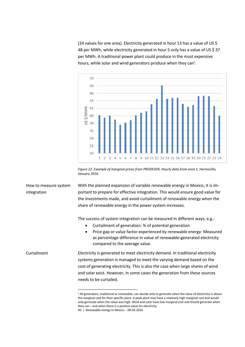
(24 values for one area). Electricity generated in hour 13 has a value of US $
48 per MWh, while electricity generated in hour 5 only has a value of US $ 37
per MWh. A traditional power plant could produce in the most expensive
hours, while solar and wind generators produce when they can1.
Figure 22. Example of marginal prices from PRODESEN. Hourly data from area 1, Hermosillo, January 2016.
With the planned expansion of variable renewable energy in Mexico, it is im-
portant to prepare for effective integration. This would ensure good value for
the investments made, and avoid curtailment of renewable energy when the
share of renewable energy in the power system increases.
The success of system integration can be measured in different ways, e.g.:
Curtailment of generation: % of potential generation
Price gap or value factor experienced by renewable energy: Measured
as percentage difference in value of renewable-generated electricity
compared to the average value.
Electricity is generated to meet electricity demand. In traditional electricity
systems generation is managed to meet the varying demand based on the
cost of generating electricity. This is also the case when large shares of wind
and solar exist. However, in some cases the generation from these sources
needs to be curtailed.
1 All generators, traditional or renewable, can decide only to generate when the value of electricity is above the marginal cost for their specific plant. A peak plant may have a relatively high marginal cost and would only generate when the value was high. Wind and solar have low marginal cost and should generate when they can – and when there is a positive value for electricity.
How to measure system
integration
Curtailment
41 | Renewable energy in Mexico - 08-05-2016
If generation in a grid section threatens to exceed the demand plus the possi-
ble export to other areas, curtailment must take place to avoid overloading of
lines. If the conventional power plants cannot reduce their output, wind and
solar generation must be reduced. It is common practice for system operators
to have control systems in place, so that e.g. selected large solar or wind parks
can be curtailed if needed. Curtailment means loss of electricity generation
(and economic costs associated with the fuel use, and extra GHG emissions
arising from the generation that could have been replaced by the potential re-
newable generation). However, if the amount of curtailment is limited, this
can be the least-cost option. In many countries with high shares of wind and
solar generation, curtailment of wind power is in the order of 1%. This can be
considered as a sign of effective integration.
Curtailment typically takes place during combination of high wind conditions
and low demand. Also crucial is the available export capacity out of the area
with wind and solar.
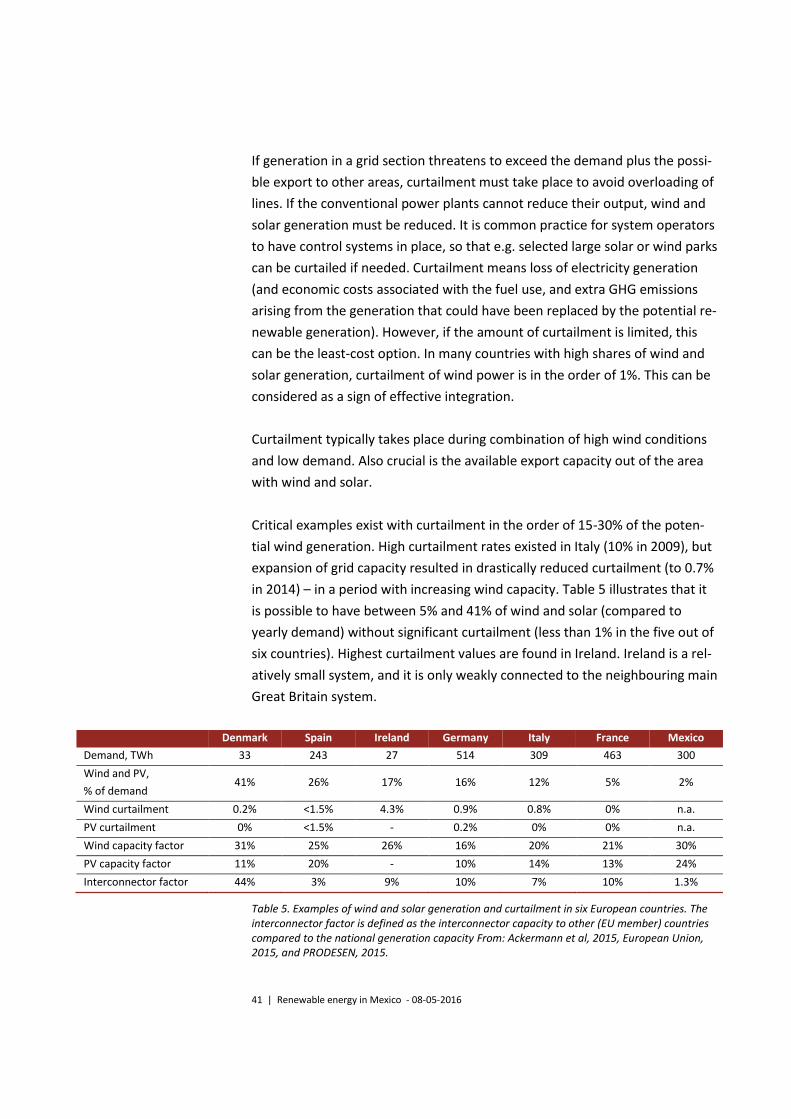
Critical examples exist with curtailment in the order of 15-30% of the poten-
tial wind generation. High curtailment rates existed in Italy (10% in 2009), but
expansion of grid capacity resulted in drastically reduced curtailment (to 0.7%
in 2014) – in a period with increasing wind capacity. Table 5 illustrates that it
is possible to have between 5% and 41% of wind and solar (compared to
yearly demand) without significant curtailment (less than 1% in the five out of
six countries). Highest curtailment values are found in Ireland. Ireland is a rel-
atively small system, and it is only weakly connected to the neighbouring main
Great Britain system.
Denmark Spain Ireland Germany Italy France Mexico
Demand, TWh 33 243 27 514 309 463 300
Wind and PV,
% of demand 41% 26% 17% 16% 12% 5% 2%
Wind curtailment 0.2% <1.5% 4.3% 0.9% 0.8% 0% n.a.
PV curtailment 0% <1.5% - 0.2% 0% 0% n.a.
Wind capacity factor 31% 25% 26% 16% 20% 21% 30%
PV capacity factor 11% 20% - 10% 14% 13% 24%
Interconnector factor 44% 3% 9% 10% 7% 10% 1.3%
Table 5. Examples of wind and solar generation and curtailment in six European countries. The interconnector factor is defined as the interconnector capacity to other (EU member) countries compared to the national generation capacity From: Ackermann et al, 2015, European Union, 2015, and PRODESEN, 2015.
42 | Renewable energy in Mexico - 08-05-2016
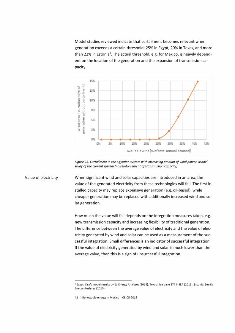
Model studies reviewed indicate that curtailment becomes relevant when
generation exceeds a certain threshold: 25% in Egypt, 20% in Texas, and more
than 22% in Estonia1. The actual threshold, e.g. for Mexico, is heavily depend-
ent on the location of the generation and the expansion of transmission ca-
pacity.
Figure 23. Curtailment in the Egyptian system with increasing amount of wind power. Model study of the current system (no reinforcement of transmission capacity).
When significant wind and solar capacities are introduced in an area, the
value of the generated electricity from these technologies will fall. The first in-
stalled capacity may replace expensive generation (e.g. oil-based), while
cheaper generation may be replaced with additionally increased wind and so-
lar generation.
How much the value will fall depends on the integration measures taken, e.g.
new transmission capacity and increasing flexibility of traditional generation.
The difference between the average value of electricity and the value of elec-
tricity generated by wind and solar can be used as a measurement of the suc-
cessful integration: Small differences is an indicator of successful integration.
If the value of electricity generated by wind and solar is much lower than the
average value, then this is a sign of unsuccessful integration.
1 Egypt: Draft model results by Ea Energy Analyses (2015). Texas: See page 377 in IEA (2015). Estonia: See Ea Energy Analyses (2010).
Value of electricity
43 | Renewable energy in Mexico - 08-05-2016
In Denmark, wind power has generated electricity 5-15% below average price,
i.e. the value factors for wind power are 0.85 to 0.95 (2002-2014)1. The close
location (including strong transmission capacity) to the large hydro capacities
in Sweden and Norway is the major reason for the low price gap. However,
model studies of system development suggest an increasing difference for the
future.
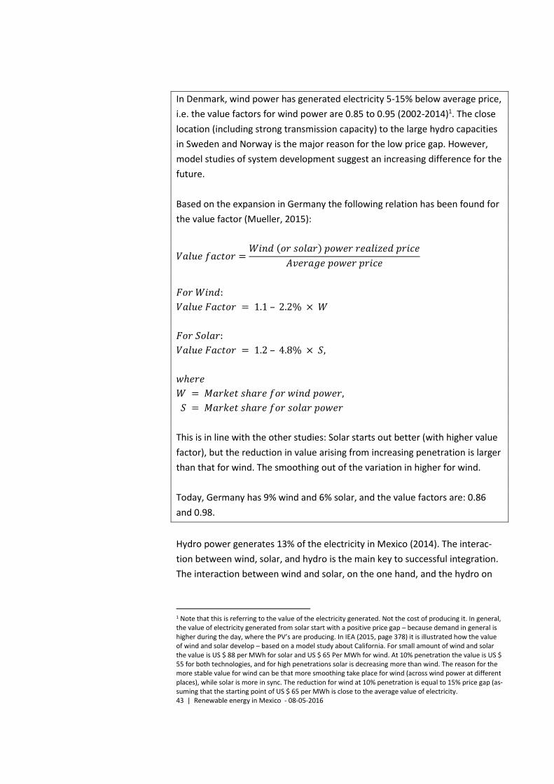
Based on the expansion in Germany the following relation has been found for
the value factor (Mueller, 2015):
𝑉𝑎𝑙𝑢𝑒 𝑓𝑎𝑐𝑡𝑜𝑟 =𝑊𝑖𝑛𝑑 (𝑜𝑟 𝑠𝑜𝑙𝑎𝑟) 𝑝𝑜𝑤𝑒𝑟 𝑟𝑒𝑎𝑙𝑖𝑧𝑒𝑑 𝑝𝑟𝑖𝑐𝑒
𝐴𝑣𝑒𝑟𝑎𝑔𝑒 𝑝𝑜𝑤𝑒𝑟 𝑝𝑟𝑖𝑐𝑒
𝐹𝑜𝑟 𝑊𝑖𝑛𝑑:
𝑉𝑎𝑙𝑢𝑒 𝐹𝑎𝑐𝑡𝑜𝑟 = 1.1 – 2.2% × 𝑊
𝐹𝑜𝑟 𝑆𝑜𝑙𝑎𝑟:
𝑉𝑎𝑙𝑢𝑒 𝐹𝑎𝑐𝑡𝑜𝑟 = 1.2 – 4.8% × 𝑆,
𝑤ℎ𝑒𝑟𝑒
𝑊 = 𝑀𝑎𝑟𝑘𝑒𝑡 𝑠ℎ𝑎𝑟𝑒 𝑓𝑜𝑟 𝑤𝑖𝑛𝑑 𝑝𝑜𝑤𝑒𝑟,
𝑆 = 𝑀𝑎𝑟𝑘𝑒𝑡 𝑠ℎ𝑎𝑟𝑒 𝑓𝑜𝑟 𝑠𝑜𝑙𝑎𝑟 𝑝𝑜𝑤𝑒𝑟
This is in line with the other studies: Solar starts out better (with higher value
factor), but the reduction in value arising from increasing penetration is larger
than that for wind. The smoothing out of the variation in higher for wind.
Today, Germany has 9% wind and 6% solar, and the value factors are: 0.86
and 0.98.
Hydro power generates 13% of the electricity in Mexico (2014). The interac-
tion between wind, solar, and hydro is the main key to successful integration.
The interaction between wind and solar, on the one hand, and the hydro on
1 Note that this is referring to the value of the electricity generated. Not the cost of producing it. In general, the value of electricity generated from solar start with a positive price gap – because demand in general is higher during the day, where the PV’s are producing. In IEA (2015, page 378) it is illustrated how the value of wind and solar develop – based on a model study about California. For small amount of wind and solar the value is US $ 88 per MWh for solar and US $ 65 Per MWh for wind. At 10% penetration the value is US $ 55 for both technologies, and for high penetrations solar is decreasing more than wind. The reason for the more stable value for wind can be that more smoothing take place for wind (across wind power at different places), while solar is more in sync. The reduction for wind at 10% penetration is equal to 15% price gap (as-suming that the starting point of US $ 65 per MWh is close to the average value of electricity.
44 | Renewable energy in Mexico - 08-05-2016
the other hand, can (as in Denmark) effectively take place through the mar-
ket. The influence of wind and solar on the hourly market prices is the motiva-
tion for the owners of hydro resources to adapt their generation. No direct
agreements are needed.
In addition, the fact that half of the Mexican electricity generation (2014)
comes from natural gas-based combined cycle units is a good starting point
for integration. These units have good dynamic properties (e.g. high ramping
rates, short starting times and low minimum loads), which has a value in rela-
tion to large amount of wind and solar1.
PV technology can be scaled in any size. A significant share of global PV expan-
sion comes as rooftop installations. In the REmap study 25% of the PV expan-
sion is expected to be rooftop installations (7.5 GW out of 30 GW).
Rooftop PV often has capacities in the order of 1 – 10 kW. These installations
can be used to cover the building’s electricity demand and may in periods
with high sun and little demand export the electricity to the local grid. If this
takes place on a large scale, it can influence the operation of the grid, e.g. in-
fluence the voltage, or even lead to export of electricity from a low voltage
grid to the higher voltage grid above this. This requires new procedures and
may also require investment in new grid capacity or control equipment.
Because of the small capacity it is typically too expensive to introduce central
control of such units. So they are operated as “must produce” units. Any ad-
justment of generation will be done on other units.
The Electricity Industry Law in Mexico defines distributed generation as units
with capacity of less than 500 kW.
3.2 Measures to improve system integration
Electricity system in Mexico, as well as in most other countries, has not been
developed with variable renewable energy in mind. Therefore, when a signifi-
cant amount of variable renewable energy is introduced, it can be relevant to
develop a number of activities to improve system integration. This can include
many aspects, e.g.:
1 In contrast, generation technologies like nuclear and large coal fired power plants are less dynamic and are often used as base load with little variation in output.
Decentral generation
45 | Renewable energy in Mexico - 08-05-2016
Increased transmission capacity (in Mexico as well as to neighbouring
countries)1
Improved market function, with all generators producing according to
marginal costs (reduce must-run and fixed payments). Optimal use of
hydro with storage. Hourly and sub-hourly dispatch. The Mexican
electricity market will start in January 2016 and has many of the fea-
tures needed to motivate maximum flexibility from all generators, in-
cluding prices that vary by the hour and locally (in the many P-nodes)
(Bloomberg, 2015)
Improved dynamic properties of traditional power plants. A number
of low-cost improvements can be made on existing coal-based power
plants to decrease minimum load, increase ramp rates and reduce
start-up costs (see Danish Energy Agency, 2015, a). A review of five
Mexican power plants describes the possibility to improve low load
operation and increase ramp rates2 (see Danish Energy Agency and
Ramboll (2014)). Dynamic market prices will motivate generators to
exhibit flexibility, also when designing new plants. Mexico has signifi-
cant capacity in hydro and gas (56% of current generation capacity).
These technologies are generally flexible and valuable assets in inte-
grating wind and solar.
Reducing the need for having traditional generators running for ancil-
lary services like voltage, reactive power and inertia3.
Demand response (price-dependent electricity demand), e.g. with
fuelshift in industry
Improved procedures for real-time planning and operation of the
electricity system near to the operational hour. This can include im-
proved procedures to activate regulating power before the imbal-
ances occur. A key feature is to utilise real-time measurements for de-
mand, wind and solar generation to create a prognosis for the next
hour’s imbalance (see Danish Energy Agency, 2015, a).
Activating new sources for balancing the system, including exchange
with neighbouring countries, activating small generators and wind
power (down regulation). This requires open and simple procedures,
e.g. not to require bidders to give symmetrical bids (both up and
down) and not to require bids to be active for long periods (an hour
1 European Union has formulated it as a goal that each member state must have at least 10% intercon-nector capacity to other member countries in 2020. The 10% is defined as the interconnector capacity to other EU member states compared to the national generation capacity. For 2030 the goal is 15%. For Mex-ico the current interconnector capacity (865 MW to USA and Belize) is 1.3% of the installed generator ca-pacity. 2 The five plants are: 1200 MW TPP "Josè Lopez Portillo; 2778 MW TPP "Plutarco Elías Calles"; 1400 MW TPP "Carbón II"; 382 MW CCGT plant "San Lorenzo"; 591 MW CCGT plant "El Sauz". 3 Denmark can today operate with medium wind speed without any central power plants running. In 15 hours on 2 September 2015 less than 12 MW of traditional (large) power plants were generating. The de-mand was between 2,800 and 4,800 MW in these hours. Investment in new units like VSC-HVDC intercon-nector, Synchronous Compensators and Static VAR compensator (SVC) makes this operation possible. Be-fore these investments 3-6 power plants were needed online at all times. See Akhmatov et al (2007).
46 | Renewable energy in Mexico - 08-05-2016
rather than a month). In the future electric vehicles may also be acti-
vated for demand response (intelligent charging).
Additional actions may be required to maintain secure system operation, e.g.:
Control systems that enable curtailment of e.g. wind and solar gener-
ation. This can be relevant for selected units, e.g. over a certain capac-
ity.
Parson et al. (2014) list best practise procedures that can be followed in study-
ing the integration of wind and solar in Mexico. These include:
Important to have access to historic wind and solar resource data to
capture temporal and spatial diversity, which will be needed to corre-
late wind generation with solar generation and electric load.
Important to collect basis data about system operation e.g., forced
outage and generation by independent power producers; perfor-
mance data and forecasts for small generators; load forecast errors
and operational load; performance data for the conventional and hy-
dropower generation fleet.
Important to have planning models for assessing expansion scenarios
for renewable and conventional generation and transmission.
Important that the market design supports efficient integration of re-
newables, e.g. with short-term dispatch and unit commitment.
Develop grid codes, e.g. so that requirements for wind turbines would
include fault ride-through, provision of reactive power, and possibly
automatic generation control, AGC.
The International Energy Agency, IEA, reviewed the flexibility of the Mexican
electricity system (IEA, 2011). Examples of the identified challenges included:
Limited interconnectors to neighbouring countries (865 MW DC).
Internal connection between the four Mexican balancing areas is lim-
ited1
1 The four synchronous areas are: The National Interconnected System (entire country, except Baja Califor-nia). In peninsula of Baja California three system is operated: Baja California, Baja California Sur and Mulegé.
47 | Renewable energy in Mexico - 08-05-2016
Examples of measures that facilitate integration of renewable energy
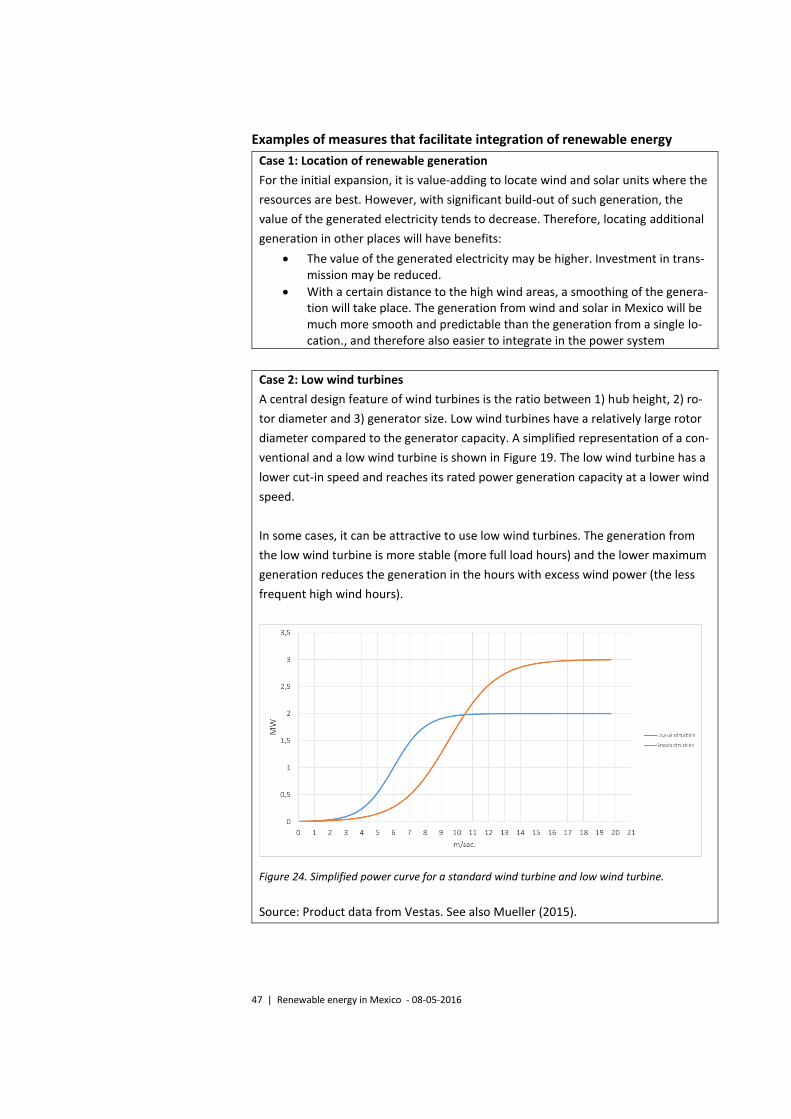
Case 1: Location of renewable generation
For the initial expansion, it is value-adding to locate wind and solar units where the
resources are best. However, with significant build-out of such generation, the
value of the generated electricity tends to decrease. Therefore, locating additional
generation in other places will have benefits:
The value of the generated electricity may be higher. Investment in trans-mission may be reduced.
With a certain distance to the high wind areas, a smoothing of the genera-tion will take place. The generation from wind and solar in Mexico will be much more smooth and predictable than the generation from a single lo-cation., and therefore also easier to integrate in the power system
Case 2: Low wind turbines
A central design feature of wind turbines is the ratio between 1) hub height, 2) ro-
tor diameter and 3) generator size. Low wind turbines have a relatively large rotor
diameter compared to the generator capacity. A simplified representation of a con-
ventional and a low wind turbine is shown in Figure 19. The low wind turbine has a
lower cut-in speed and reaches its rated power generation capacity at a lower wind
speed.
In some cases, it can be attractive to use low wind turbines. The generation from
the low wind turbine is more stable (more full load hours) and the lower maximum
generation reduces the generation in the hours with excess wind power (the less
frequent high wind hours).
Figure 24. Simplified power curve for a standard wind turbine and low wind turbine.
Source: Product data from Vestas. See also Mueller (2015).
48 | Renewable energy in Mexico - 08-05-2016
Case 3: Procedure in relation to the activation of reserves
The Danish electricity demand is 33 TWh/year with a peak demand of 6,200 MW.
The installed wind power capacity in Denmark is 4.800 MW and solar is 620 MW.
Interconnectors of 6,000 MW exist to the neighbouring countries (Sweden, Norway
and Germany).
Automatic reserves (primary and secondary) are central to maintaining a stable
electricity system. When a fault happens, e.g. loss of a power plant, the frequency
and exchanges in the synchronous system will change, and the automatic reserves
will instantaneously kick in and replace the missing generation. Manual reserves
are then activated by the control room to release the primary and secondary re-
serves.
A common practice is to activate reserves “in real time”, as the events occur. If the
main drivers for imbalances are random and essentially unpredictable outages of
generators, this is a relevant procedure.
As the installed wind power capacity in Denmark was increasing, however, Ener-
ginet.dk started developing a system to predict the imbalances. A system called
Operational planning system, DPS, was created. The system collects data from nu-
merous sources and presents a single curve for the operators in the TSO control
room. The curve shows the predicted imbalance in the system.
The data used to collate the predicted imbalance in the system is as follows:
Wind power. Each five minutes a new prognosis is produced. The frequent
updating uses online measurements to correct the meteorological predic-
tions (these are only updated each four hours). The online measurements
represent a large sample of all the wind power units and are up-scaled to
represent the entire generation.
Solar power. A similar system is used to predict the power from the PV
systems.
Demand. Also for demand, the prognosis is frequently updated based on
online measurements (of generation and import/export).
Plans for the market participants. Detailed plans are received e.g. for all
major generators. These plans have information about the expected gen-
eration in five minute intervals1.
The predicted imbalance curve will cover the next 12 hours. When significant im-
balances are foreseen, the control room operators will:
Discuss with neighbouring TSO’s if imbalances can be exchanged (at no
cost), e.g. if Sweden has a positive balance and West Denmark a negative
balance – and if transmission capacity is available, the two imbalances can

49 | Renewable energy in Mexico - 08-05-2016
offset each other. This also applies to the exchange between the two Dan-
ish areas (DK1 and DK2, West and East – that are a part of two different
synchronous systems).
Activate tertiary reserves (regulating power) to outweigh the expected im-
balance. This is done from a common Nordic system (with bids from four
countries), the NOIS list.
The traditional procedures for activating reserves can be called reactive, while the
Energinet.dk approach can be called proactive. In popular terms the new procedure
can be described as “driving looking through the front window” in contrast to “driv-
ing looking in the rear view mirror”.
1 This is in contrast to the spot market, Nord Pool Spot, which operates with hourly values.
50 | Renewable energy in Mexico - 08-05-2016
Case 4: System-wide and regional need for reserves
The Danish TSO, Energinet.dk, reports that the introduction of 4,800 MW wind and
600 MW solar power has not yet influenced the amount of planned reserves used in
the system. To understand this statement a simple presentation for the basic
framework of having reserves is presented.
A small islanded system
In an isolated system the largest unit may be 600 MW. Such a system (based on the
N-1 principle) would need to have 600 MW primary reserve, no secondary reserve1
and 600 MW of tertiary reserve. If the tertiary reserve can be activated within 15
minutes, then this system can withstand one big fault – and after 15 minutes an-
other one. If two large faults occur with less than 15 minutes apart, the reserves
would not be able to manage the lack of generation and load shedding must be ac-
tivated (e.g. with under frequency relays).
A two-area system
Imagine a system with two equally large areas A and B. The largest fault is still 600
MW. Based on the above principle, the total amount of primary reserve must be
600 MW and this could be divided equally to each of the two areas (2 x 300 MW).
The secondary reserve must be 600 MW in each system (assuming that each sys-
tem has a unit of this size). Each system may also need 600 MW of tertiary re-
serves.
UCTE – reserves, wind and solar
The UCTE is a large synchronous system, from Denmark in North, to Portugal in the
South/West and Italy in the South: 2,300 TWh, 400,000 MW peak load, 100,000
MW wind and 72,000 MW solar. In this system 3,000 MW is considered at the di-
mensioning error. West Denmark must cover a fraction of this, computed as the
fraction of demand: 23 MW as primary reserve.
In West Denmark the dimensioning error is 600 MW, so this is also the required
amount of tertiary reserve. For tertiary reserve (regulating power), the situation is
that there typically is a large surplus of this. The hydro power in the other Nordic
countries typically has a large unused capacity. Depending on the expected opera-
tion and availability of the cross-border transmission capacity, Energinet.dk may re-
serve capacity for the tertiary reserve. Typically, Energinet.dk reserves 200-300
MW upregulation and no downregulation (Denmark, West, 2014-2015).
The dimensioning error represents a sudden incident. In a fraction of a second
3,000 MW (UCTE) generation can be lost, e.g. if a short circuit isolates a power
plant from the grid (In Denmark the dimension fault is 600 MW).
51 | Renewable energy in Mexico - 08-05-2016
Energinet.dk highlights that the introduction of wind and solar power has not in-
creased the need for reserves in UCTE or Denmark. In Denmark wind and solar is
5,400 MW, and in UCTE it is in the order of 172,000 MW.
The background is that prognosis errors from wind and solar may be large on a day-
ahead perspective, but will gradually be reduced as the time is approaching the op-
erating hour and second. The hour-ahead error will be much smaller than the day-
ahead error. And, below the hour-ahead the actual (and partly un-predicted) gen-
eration from wind and solar will influence the frequency and the flow on the inter-
connectors. Thereby reserves will be activated and balance will be re-established.
So, despite the large size of the wind and solar capacity the sudden (unpredicted)
change in output is still considered smaller than 3,000 MW (the dimensioning er-
ror) on UCTE scale.
On a day-ahead scale the typical forecast error for wind power in Denmark is in the
order of 20% (Mean Absolute Percentage Error, MAPE); however, this is continu-
ously reduced as the time is approaching the operating second. While the output
from a single wind farm may change rapidly, the aggregated output from a large
area as UCTE (2,500 km from North to South) will develop quite smoothly. With
continuously expanding capacity of wind and solar, at some point this will result in
extra need for reserves. However, UCTE is not at this point, yet.
3.3 Possible actions in relation to system integration
Possible actions:
The future Renewable Energy Outlook (REO) could report on system
integration. Together with information about the power generated
from renewable sources the year before, information about curtail-
ment and the realised price gap / value factor could be reported. Price
information will be available from market systems going forward. Re-
newable generation must be recorded per P-node to compute the
price gap.
Evaluate possible expansion of transmission capacity – both internal
and in relation to the neighbouring countries – in light of the expan-
sion of renewable energy.
Secure that market systems as well as procedures for ancillary ser-
vices are efficient and support the flexibility of the system
1 The purpose of the secondary reserve is to locate in which control area the fault has occurred. With only one control area, there is no need for the secondary reserve.
52 | Renewable energy in Mexico - 08-05-2016
References to chapter 3
Ackermann, T., E. M. Carlini, B. Ernst, F. Groome, A. Orths, J. O’Sullivan, M.T.
Rodriquez and V. Silva (2015): Integrating variable Renewables in Europe. IEEE
November 2015.
Akhmatov, V., C. Rasmussen, P.B. Eriksen and J. Pedersen (2007): Technical
Aspects of Status and Expected Future Trends for Wind Power in Denmark.
Wind Energy, 10:31–49.
Bloomberg (2015): AMER – Latin America – Wind, Solar, Power
City (2013): Energy Darwinism. City GPS: Global Perspectives & Solutions.
Danish Energy Agency (2015, a): Flexibility in the Power System – Danish and
European experiences.
Danish Energy Agency (2015, b): Power markets and power sector planning in
Europe – Lessons learnt for China.
Ea Energy Analyses (2010): Wind Power in Estonia. An analysis of the possibili-
ties and limitations for wind power capacity in Estonia within the next 10
years.
http://www.ea-energianalyse.dk/reports/1001_Wind_Power_in_Estonia.pdf
Ea Energy Analyses (2015): The Danish Experience with Integrating Variable
Renewable Energy. Study on behalf of Agora Energiewende.
EcoFys (2015): Power System Flexibility Strategic Roadmap. Preparing power
systems to supply reliable power from variable energy resource
European Union (2015): Energy Union Package. Communication from the
Commission to the European Parliament and the Council. Achieving the 10%
electricity interconnection target. Making Europe's electricity grid fit for 2020.
COM(2015) 82 final
ec.europa.eu/priorities/energy-union/docs/interconnectors_en.pdf
Holttinen, H. et al (2013): Summary of experiences and studies for Wind
Integration – IEA Wind Task 25. WIW2013 workshop London, 22-24 Oct, 2013.
www.ieawind.org/task_25/PDF/W1W/WIW13_Task25_Summarypaper_final.pdf
53 | Renewable energy in Mexico - 08-05-2016
IEA Task 25 Fact Sheet: Wind Integration Issue.
http://www.ieawind.org/index_page_postings/task25/FactSheet_1_121014.pdf
IEA (2011): Harnessing Variable Renewables. A Guide to the Balancing Chal-
lenge.
IEA (2014): The Power of Transformation: Wind, Sun and the Economics of
Flexible Power Systems, International Energy Agency, Paris, 2014.
IEA (2015): World Energy Outlook.
Milligan, M, B. Kirby, H. Holttinen, J. Kiiluoma, A. Estanqueiro, S.Martin-Marti-
niz, E. Gomaz-Lazaro, I. Pineda and C. Smith (2013): “Wind Integration Cost
and Cost-Causation”. 12th Wind Integration Workshop
http://www.nrel.gov/docs/fy14osti/60411.pdf
Mueller, S. (2015): System-friendly wind power. A Grid Integration of Variable
Renewables (GIVAR) modelling analysis. GIVAR Advisory Group meeting, Paris,
26 October 2015.
Parsons, B., J., J. Cochran, A. Watson, J. Katz, R. Bracho (2014): Renewable
Electricity Grid Integration Roadmap for Mexico: Supplement to the IEA Expert
Group Report on Recommended Practices for Wind Integration Studies. Ec-
Leds Enhancing Capacity for Low Emission Development Strategies. Renewa-
ble Electricity Grid Integration Roadmap for Mexico: Supplement to the IEA
Expert Group Report on Recommended Practices for Wind Integration Stud-
ies.
Ramboll (2014): Workshop with CFE. Flexibility of Mexican power plants.
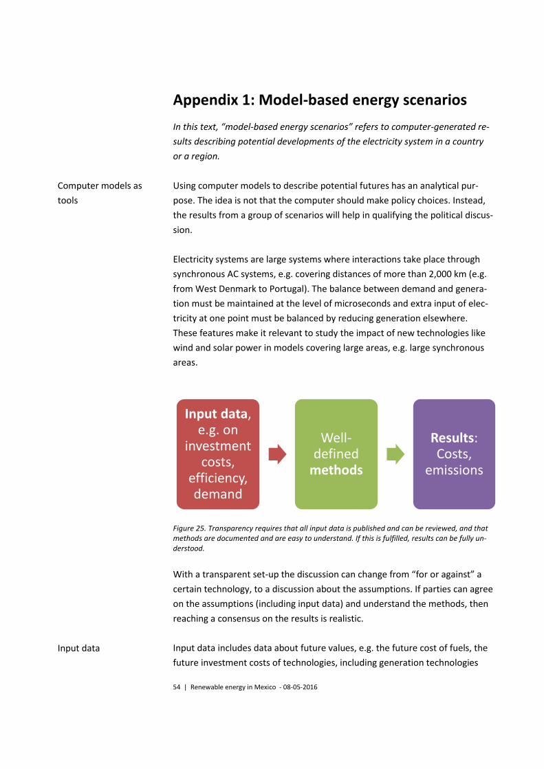
54 | Renewable energy in Mexico - 08-05-2016
Appendix 1: Model-based energy scenarios
In this text, “model-based energy scenarios” refers to computer-generated re-
sults describing potential developments of the electricity system in a country
or a region.
Using computer models to describe potential futures has an analytical pur-
pose. The idea is not that the computer should make policy choices. Instead,
the results from a group of scenarios will help in qualifying the political discus-
sion.
Electricity systems are large systems where interactions take place through
synchronous AC systems, e.g. covering distances of more than 2,000 km (e.g.
from West Denmark to Portugal). The balance between demand and genera-
tion must be maintained at the level of microseconds and extra input of elec-
tricity at one point must be balanced by reducing generation elsewhere.
These features make it relevant to study the impact of new technologies like
wind and solar power in models covering large areas, e.g. large synchronous
areas.
Figure 25. Transparency requires that all input data is published and can be reviewed, and that methods are documented and are easy to understand. If this is fulfilled, results can be fully un-derstood.
With a transparent set-up the discussion can change from “for or against” a
certain technology, to a discussion about the assumptions. If parties can agree
on the assumptions (including input data) and understand the methods, then
reaching a consensus on the results is realistic.
Input data includes data about future values, e.g. the future cost of fuels, the
future investment costs of technologies, including generation technologies
Input data, e.g. on
investment costs,
efficiency, demand
Well-defined
methods
Results: Costs,
emissions
Computer models as
tools
Input data
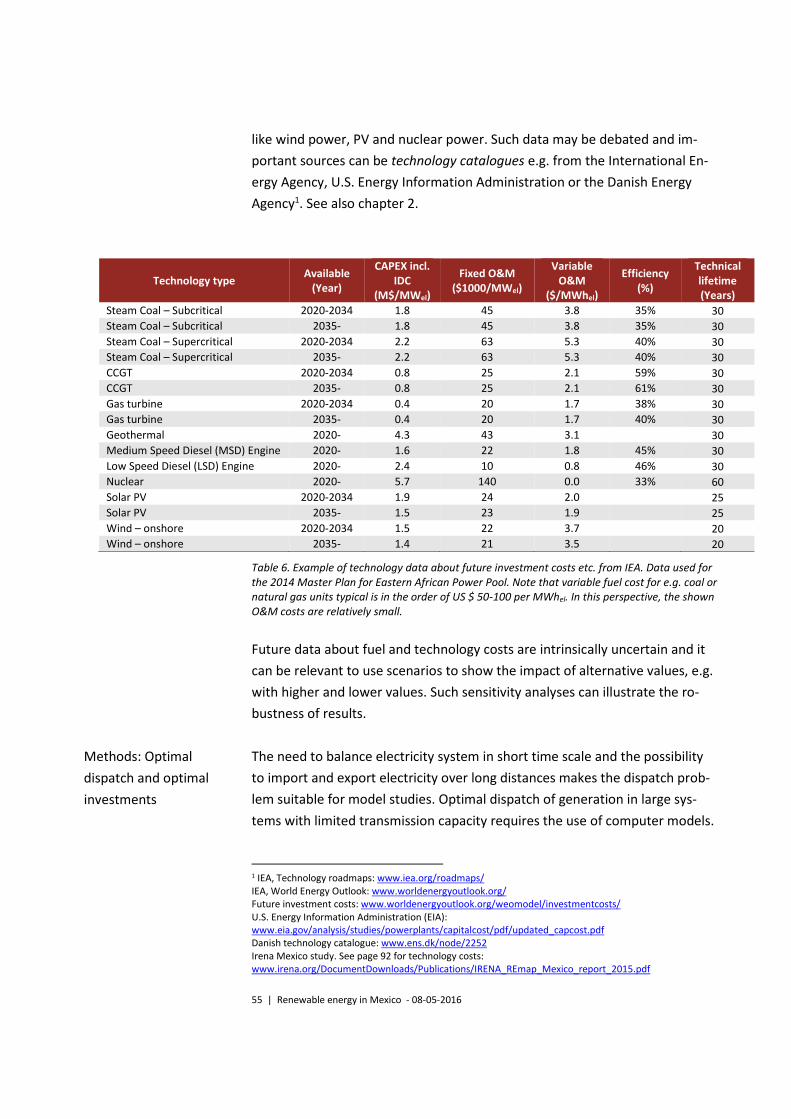
55 | Renewable energy in Mexico - 08-05-2016
like wind power, PV and nuclear power. Such data may be debated and im-
portant sources can be technology catalogues e.g. from the International En-
ergy Agency, U.S. Energy Information Administration or the Danish Energy
Agency1. See also chapter 2.
Technology type Available
(Year)
CAPEX incl. IDC
(M$/MWel)
Fixed O&M ($1000/MWel)
Variable O&M
($/MWhel)
Efficiency (%)
Technical lifetime (Years)
Steam Coal – Subcritical 2020-2034 1.8 45 3.8 35% 30
Steam Coal – Subcritical 2035- 1.8 45 3.8 35% 30
Steam Coal – Supercritical 2020-2034 2.2 63 5.3 40% 30
Steam Coal – Supercritical 2035- 2.2 63 5.3 40% 30
CCGT 2020-2034 0.8 25 2.1 59% 30
CCGT 2035- 0.8 25 2.1 61% 30
Gas turbine 2020-2034 0.4 20 1.7 38% 30
Gas turbine 2035- 0.4 20 1.7 40% 30
Geothermal 2020- 4.3 43 3.1 30
Medium Speed Diesel (MSD) Engine 2020- 1.6 22 1.8 45% 30
Low Speed Diesel (LSD) Engine 2020- 2.4 10 0.8 46% 30
Nuclear 2020- 5.7 140 0.0 33% 60
Solar PV 2020-2034 1.9 24 2.0 25
Solar PV 2035- 1.5 23 1.9 25
Wind – onshore 2020-2034 1.5 22 3.7 20
Wind – onshore 2035- 1.4 21 3.5 20
Table 6. Example of technology data about future investment costs etc. from IEA. Data used for the 2014 Master Plan for Eastern African Power Pool. Note that variable fuel cost for e.g. coal or natural gas units typical is in the order of US $ 50-100 per MWhel. In this perspective, the shown O&M costs are relatively small.
Future data about fuel and technology costs are intrinsically uncertain and it
can be relevant to use scenarios to show the impact of alternative values, e.g.
with higher and lower values. Such sensitivity analyses can illustrate the ro-
bustness of results.
The need to balance electricity system in short time scale and the possibility
to import and export electricity over long distances makes the dispatch prob-
lem suitable for model studies. Optimal dispatch of generation in large sys-
tems with limited transmission capacity requires the use of computer models.
1 IEA, Technology roadmaps: www.iea.org/roadmaps/ IEA, World Energy Outlook: www.worldenergyoutlook.org/ Future investment costs: www.worldenergyoutlook.org/weomodel/investmentcosts/ U.S. Energy Information Administration (EIA): www.eia.gov/analysis/studies/powerplants/capitalcost/pdf/updated_capcost.pdf Danish technology catalogue: www.ens.dk/node/2252 Irena Mexico study. See page 92 for technology costs: www.irena.org/DocumentDownloads/Publications/IRENA_REmap_Mexico_report_2015.pdf
Methods: Optimal
dispatch and optimal
investments
56 | Renewable energy in Mexico - 08-05-2016
Optimal dispatch is well defined: if the marginal generation costs are known
for each generator, one solution will have the lowest total costs. The marginal
cost of traditional power plants is defined as the fuel price divided by the effi-
ciency. Wind and solar power have high investment cost, but their marginal
generation costs are close to zero. These technologies will produce when the
sun is shining or the wind is blowing1. Hydro plants with reservoir also have a
low marginal cost. However, the optimal dispatch of such hydro plants must
consider that the units are restricted by the inflow of water. Optimal dispatch
of hydropower means optimal use of the available water across a longer pe-
riod, e.g. a year. The optimal use of hydropower is to optimise (maximise) the
value of the electricity generated.
In the simplest set-up, each hour is considered independently, start-up and
stop costs are ignored. These costs could be included in the modelling to
make the dispatch more realistic, since power plants that are running in one
hour are likely to continue generation in the next hour. Using such unit com-
mitment costs will increase computer time and the more detailed dispatch is
often not needed in studies of future situations as the change in the total an-
nual system costs may not change significantly. Simulation to be used in the
daily operation can be more detailed than in future scenario analyses. In fu-
ture scenario analyses, unit commitment may not be applied and representa-
tive weeks can be included instead of the full number of hours of each year
(8760).
Scenarios may include model-based investments in generation and transmis-
sion. Model-based investment may take place in a simplified way, e.g. the
model may invest if the annualised costs of investments is less that the bene-
fit in the same year. The set-up can be called myopic because the future use
of the investment is not included.
Scenarios can be defined to support the political discussion. They are not
meant as predictions, but as possible futures. Models are simplifications of
real life and the absolute results may not always be accurate. However, the
difference between two scenarios may be more accurate, e.g. changing an in-
put parameter will produce differences both in dispatch as well as invest-
ments.
1 In situations with large must produce generation the electricity price may be negative and it is relevant to curtail wind and solar.
Scenarios
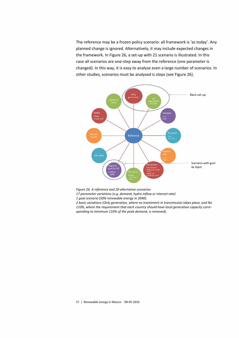
57 | Renewable energy in Mexico - 08-05-2016
The reference may be a frozen policy scenario: all framework is ‘as today’. Any
planned change is ignored. Alternatively, it may include expected changes in
the framework. In Figure 26, a set-up with 21 scenario is illustrated. In this
case all scenarios are one-step away from the reference (one parameter is
changed). In this way, it is easy to analyse even a large number of scenarios. In
other studies, scenarios must be analysed is steps (see Figure 26).
Figure 26. A reference and 20 alternative scenarios: 17 parameter variations (e.g. demand, hydro inflow or interest rate) 1 goal scenario (50% renewable energy in 2040). 2 basic variations (Only generation, where no investment in transmission takes place, and No 110%, where the requirement that each country should have local generation capacity corre-sponding to minimum 110% of the peak demand, is removed).
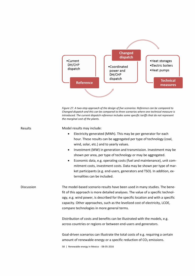
58 | Renewable energy in Mexico - 08-05-2016
Figure 27. A two-step approach of the design of five scenarios: Reference can be compared to Changed dispatch and this can be compared to three scenarios where one technical measure is introduced. The current dispatch reference includes some specific tariffs that do not represent the marginal cost of the plants.
Model results may include:
Electricity generated (MWh). This may be per generator for each
hour. These results can be aggregated per type of technology (coal,
wind, solar, etc.) and to yearly values.
Investment (MW) in generation and transmission. Investment may be
shown per area, per type of technology or may be aggregated.
Economic data, e.g. operating costs (fuel and maintenance), unit com-
mitment costs, investment costs. Data may be shown per type of mar-
ket participants (e.g. end-users, generators and TSO). In addition, ex-
ternalities can be included.
The model-based scenario results have been used in many studies. The bene-
fit of this approach is more detailed analyses. The value of a specific technol-
ogy, e.g. wind power, is described for the specific location and with a specific
capacity. Other approaches, such as the levelized cost of electricity, LCOE,
compare technologies in more general terms.
Distribution of costs and benefits can be illustrated with the models, e.g.
across countries or regions or between end-users and generators.
Goal-driven scenarios can illustrate the total costs of e.g. requiring a certain
amount of renewable energy or a specific reduction of CO2 emissions.
Results
Discussion
59 | Renewable energy in Mexico - 08-05-2016
In this text, the focus has been on model-based scenarios. Please note that
the scenario technique can be used in many ways. In some cases scenarios are
used to describe possible futures in a qualitative way, see ENTSO-E (2015),
Danish Energy Agency (2014) and EcoGrid (2009).
References
Cowi and Ea Energy Analyses (2014): System integration of wind power by use
of the DH/CHP systems in North-East China.
Danish Energy Agency (2014). Energy scenarios for 2020, 2035 and 2050. www.ens.dk/sites/ens.dk/files/undergrund-forsyning/el-naturgas-varmeforsyning/Energianalyser/nyeste/energiscenar-
ier_uk.pdf
Ea Energy Analyses (2011): Costs and benefits of implementing renewable en-
ergy policy in South Africa. Results of a power system model of the South Afri-
can electricity system. www.ea-energianalyse.dk/reports/1132_costs_benefits_of_implementing_re_in_south_africa.pdf
Ea Energy Analyses (2013): Optimal investments in generation and transmis-
sion capacity in the Baltic Sea Region - 2020-2050. ea-energianalyse.dk/presentations/11XX_optimal_investments_generation_transmission_baltic_sea_region.pdf
Ea Energy Analyses, Energinet.dk and EAPP (2014): EAPP regional power sys-
tem master plan.
Ea Energy Analyses (2014): Electricity Grid Expansion in the Context of Renew-
ables Integration in the Baltic Sea Region. www.ea-energianalyse.dk/reports/1363_electricity_grid_expansion_renewables_integration_bsr.pdf
EcoGrid (2009): Steps toward a Danish power system with 50% wind energy. energinet.dk/SiteCollectionDocuments/Engelske%20dokumenter/Forskning/EcoGrid.dk%20-%20WP3%20International%20scenarios.pdf
ENTSO-E (2015): ENTSO-E Scenario Outlook & Adequacy Forecast (SO&AF)
2015 www.entsoe.eu/publications/system-development-reports/adequacy-forecasts/Pages/default.aspx
Examples of scenario studies:
ea-energianalyse.dk/themes/modellering_af_energisystemer.html
www.ea-energianalyse.dk/themes/energy_scenarios.html
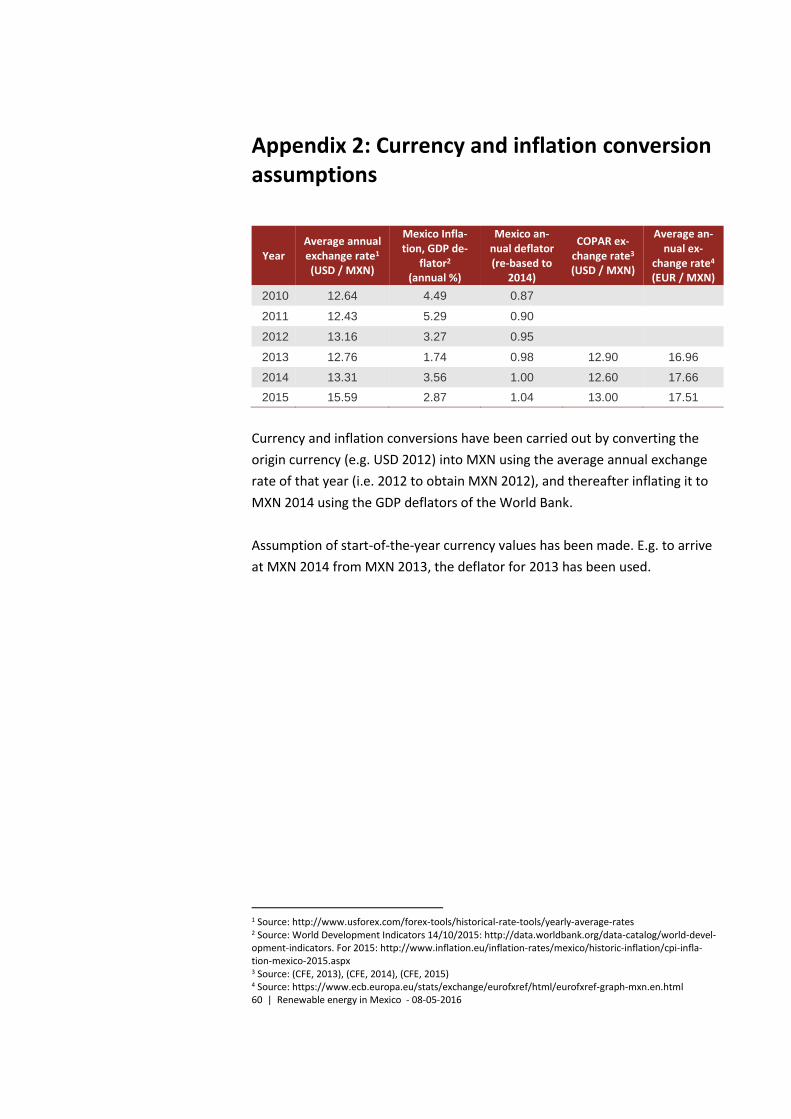
60 | Renewable energy in Mexico - 08-05-2016
Appendix 2: Currency and inflation conversion assumptions
Year Average annual exchange rate1 (USD / MXN)
Mexico Infla-tion, GDP de-
flator2 (annual %)
Mexico an-nual deflator (re-based to
2014)
COPAR ex-change rate3 (USD / MXN)
Average an-nual ex-
change rate4 (EUR / MXN)
2010 12.64 4.49 0.87
2011 12.43 5.29 0.90
2012 13.16 3.27 0.95
2013 12.76 1.74 0.98 12.90 16.96
2014 13.31 3.56 1.00 12.60 17.66
2015 15.59 2.87 1.04 13.00 17.51
Currency and inflation conversions have been carried out by converting the
origin currency (e.g. USD 2012) into MXN using the average annual exchange
rate of that year (i.e. 2012 to obtain MXN 2012), and thereafter inflating it to
MXN 2014 using the GDP deflators of the World Bank.
Assumption of start-of-the-year currency values has been made. E.g. to arrive
at MXN 2014 from MXN 2013, the deflator for 2013 has been used.
1 Source: http://www.usforex.com/forex-tools/historical-rate-tools/yearly-average-rates 2 Source: World Development Indicators 14/10/2015: http://data.worldbank.org/data-catalog/world-devel-opment-indicators. For 2015: http://www.inflation.eu/inflation-rates/mexico/historic-inflation/cpi-infla-tion-mexico-2015.aspx 3 Source: (CFE, 2013), (CFE, 2014), (CFE, 2015) 4 Source: https://www.ecb.europa.eu/stats/exchange/eurofxref/html/eurofxref-graph-mxn.en.html