REMOTE SENSING: LIDAR 1

REMOTE SENSING: LIDAR 2

Cover Image: Airborne LiDAR point cloud data collected in the Democratic Republic of the Congo in 2015

© WWF/BMUB/KFW/Southern Mapping Company

Special thanks for review and support to: Sverre Lundemo, Pablo Izquierdo, Evi Korakaki, Naikoa Aguilar-Amuchastegui, and Lauri Korhonen.

Funding for this report was provided by WWF-UK.

WWF is one of the world’s largest and most experienced independent conservation organizations, with over 5 million supporters and a global network active in more than 100 countries. WWF’s mission is to stop the degredation of the planets natural environment and to build a future in which humans live in harmony with nature by conserving the worlds biological diversity, ensuring that the use of renewable natural resources is sustainable, and promoting the reduction of pollution and wasteful consumption.

Markus Melin, Aurélie C. Shapiro, and Paul Glover-Kapfer. 2017.WWF Conservation Technology Series 1(3). WWF-UK, Woking, United Kingdom.

REMOTE SENSING: LIDAR 3

What is LiDAR?LiDAR (light detection and ranging) is a remote sensing method that uses a laser to measure distances. Pulses of light are emitted from a laser scanner, and when the pulse hits a target, a portion of its photons are reflected back to the scanner. Because the location of the scanner, the directionality of the pulse, and the time between pulse emission and return are known, the 3D location (XYZ coordinates) from which the pulse reflected is calculable. The laser emits millions of such pulses, and records from whence they reflect producing a highly precise 3D point cloud (model) which can be used to estimate the 3D structure of the target area. See Chapters 2 and 3 for more details.

How are LiDAR data collected?Most often, the scanning laser is mounted in an aircraft – typically a fixed-wing airplane although increasingly in drones – and scans the ground along its route or direction of flight. Occasionally scanning lasers are mounted on a tripod or vehicle for terrestrial based laser (TLS) scans. For additional information, see Chapter 2.

What can LiDAR data do?LiDAR data provide a detailed 3D model of the target area, including its terrain, topography, and vegetation. In turn the digital terrain model of the ground surface can be used to derive a range of additional products including models of slope or visibility, and the 3D data on vegetative structure can be used for a broad range of applications within forestry and ecological contexts. See Chapter 5 for more information and additionalLiDAR applications.

Are LiDAR and Airborne Laser Scanning the same thing – terminology?Airborne laser scanning, or ALS, is simply LiDAR whilst airborne, i.e. collecting LiDAR data from an aircraft. Alternatively, if the LiDAR scanner is on a tripod, we would refer to the method as Terrestrial Laser Scanning, or TLS.

What is the difference between a pulse and an echo?A pulse is what the scanning laser emits. The pulse can be thought of as a clump of timestamped photons. As the pulse hits a target, some of its photons reflect back and are recognised by the LiDAR device: an echo was received. Therefore, the source of an echo is a location that was hit by a pulse and from which photons were reflected. One emitted pulse can, and often does, yield multiple echoes. See Chapter 2 for additional details.

What is the resolution of LiDAR data?Most often, the data that is freely distributed has a density between 0.8 – 3 pulses / m2.This is termed the pulse density. Note that pulse density refers to emitted pulses / m2.A common term is also echo- or return density, which refer to echoes / m2; one emitted pulse can yield multiple echoes. If an airplane flies at a low altitude of 200-600 meters the data may have a pulse density of 10 pulses / m2. Terrestrial Laser Scanning data easily results in point densities of at least hundreds of pulses per square meter.

LIDAR FAQ

REMOTE SENSING: LIDAR 4

Do I need LiDAR or will other data suffice?Depending on your aim, photogrammetry, satellite or aerial imagery may suffice. However, if you require high precision 3D structural information about a target area (be it forest or terrain), then LiDAR provides excellent precision, albeit at a relatively high cost. See Chapter 5 for examples of LiDAR applications. In some cases, LiDAR data are used in conjunction with other remote sensing data to produce insights neither data are able to achieve alone.

How can I acquire LiDAR data?Many countries have already collected vast amounts of LiDAR data for the purposes of topographic mapping and forestry and in many cases, these data are freely available. SeeChapter 8 for a list of available datasets. If LiDAR data are not available for your area of interest, you need to consider whether it is necessary to invest in its collection.

How much does it cost to collect LiDAR data?With ALS or airborne LiDAR, the biggest expense is associated with the operation of the aircraft, which is dependent on issues such as distance of the study site from the nearest airport (which determines which types of aircraft can be used), fuel costs, altitude, pilot time, and weather. As such, these prices vary as a function of geography and time as well as the size of the target area, making general estimates difficult. The cost typically declines per unit area as the size of the surveyed area increases and can be quite cost effective for large scales. Terrestrial laser scanning systems are becoming more compact and affordable, and the availability of drones are decreasing the cost of collecting small-scale LiDAR.

What do LiDAR data consist of?The data contains information about each received echo. For example, in a text (.txt)format the data is often structured so that one row holds information from one echo - its XYZ coordinates, intensity, and order in the case of multiple echoes. See Chapter 3.2 for more information.

How are LiDAR data different from aerial or satellite imagery?Similar to a photograph without a flash, aerial and satellite imagery are considered passive in that they record information from reflected sunlight. In other words, the light source is external because the sensor does not emit anything. In contrast, with its emitted pulses of light, LiDAR is an active remote sensing method. Furthermore, whereas imagery contains spectral data, LiDAR data do not; rather LiDAR data contain the structural information in the form of 3D coordinates, and the intensity of each echo. See Chapter 3.2 for more on LiDAR data and Chapter 9 for differences between LiDAR and imagery.

Do I need to ground-truth LiDAR data?Because LiDAR data are not interpreted in the same sense as imagery and is highly precise (most commonly to within 5-15 cm) ground-truthing of the point cloud structure for 3D mapping is generally not necessary. That being said, if you are studying something other than physical terrain, such as whether a certain echo pattern came from a particular species of tree, or are using LiDAR data in combination with other remotely sensed and interpreted data, then ground-truthing may be necessary.

REMOTE SENSING: LIDAR 5

What format do the data come in and how large are the datasets?Most often, LiDAR data come in compressed LAS/LAZ format. LAS format is a standard format for LiDAR data storage, and LAZ format is a compressed format of LAS. For example, the National Land Survey of Finland distributes their LiDAR data in LAZ files, where a single file contains LiDAR data from a 3 x 3 km area. The compressed LAZ file can be as small as 50 megabytes, but when uncompressed and converted into a text file, which may have tens of millions of rows (one for each echo), could be on the order of many gigabytes. See Chapter 3.2 for more information.

Can the LiDAR data format be changed?The data can be converted to many other formats, including plain ASCII files and ESRI shapefiles. The only practical limitation is the size: a point shapefile with 20 million points would be very slow to load and process in GIS software. Many common programs for processing LiDAR offer tools for conversion. See Chapter 7 for additional information.

What programs are available for processing LiDAR data?There are many programs that have been tailored specifically for processing and analysingLiDAR data, and the most common GIS and remote sensing programs are able to processLiDAR data in LAS/LAZ format as well. See Chapter 7 for information about common programs for processing and analysing LiDAR data.

Can LiDAR data be used without any processing?Generally no. In the core of the processing chain is the need to scale the heights(Z-coordinates) of the LiDAR echoes to ground level so that each echo has a Z-coordinate indicating its height above ground level, though often the service provider that collects the data can process the data for a fee. This is achieved by first separating the ground echoes from the other echoes, then by creating a terrain model from the ground echoes and finally, by subtracting this terrain model from the height of the echo in the LiDAR data. This effectively scales all the echoes at above-ground-level scale. The basics of this process are explained in Chapter 4.1.

How do I use LiDAR data in my analyses?Typically, the first step involves delineating your target area and extracting the relevant, manageable data from the larger LiDAR data set. You will then frequently need to rescale the data as described in the question above. Next, you calculate relevant metrics from the available 3D point clouds, a common example being canopy height or density. Although time consuming and relatively complex to work with, the adaptability of LiDAR data to suit individual needs and derive myriad metrics of 3D structure is its beauty. See Chapter 5 for examples of how the data have been used in different disciplines.

Can the point cloud data be converted into rasters like satellite images, for instance?There is no reason why LiDAR data cannot be converted into rasters, but more commonlyLiDAR data are used to derive habitat structural variables, which are then converted to rasters. For example, in some forestry cases it is common to grid the study area into 16 x16 meter grid cells and to extract LiDAR data within each cell. Variables of forest structure are calculated from the point clouds within each cell, and these variables are then incorporated into a raster with cells of the same dimensions. Common raster products from LiDAR are digital terrain and canopy height models.

REMOTE SENSING: LIDAR 6

Image: © G.Asner/Carnegie Institution for Science

Light Detection and Ranging (LIDAR) provides

high precision data on the 3D structure of forests,

enabling landscape level mapping of forest change

REMOTE SENSING: LIDAR 7

1 Preface 8 1.1 The aim of this guide 8 1.2 The structure of this guide 8

2 Introduction to LiDAR remote sensing 9 2.1 Terminology 9 2.2 History of LiDAR 10 2.3 The method – what is LiDAR? 10

3 Understanding the data 15 3.1 Types of LiDAR 15 3.2 Format and structure 15

4 Data processing and products 17 4.1 Aim of data processing 17 4.2 Common LiDAR data products 18

5 LiDAR Applications 22 5.1 Forestry, vegetation structure 22 5.2 Analysis of land cover, topography and hydrology 24 5.3 Ecological applications 24 5.3.1 Volant and canopy species 24 5.3.2 Terrestrial species 25 5.3.3 Mapping suitable habitat 25 5.3.4 Estimating canopy cover and leaf area index 25 5.3.5 Detecting forest change 25 5.4 Forest biomass mapping 26 5.5 Bathymetry 26

6 LiDAR horizons 28 6.1 Multi-wavelength (or multispectral) LiDAR 28 6.2 Spaceborne systems 28

7 LiDAR software 29 8 Data acquisition and availability 32

9 LiDAR strengths and weaknesses 34 9.1 LiDAR weaknesses in brief 34 9.2 LiDAR strengths in brief 34 9.3 Summary of strengths and weaknesses 35

10 Bibliography 36

TABLE OF CONTENTS

REMOTE SENSING: LIDAR 8

PREFACE1.1 The aim of this guideThreats like climate change, habitat destruction and degradation, and pollution are ubiquitous,requiring global-scale solutions. Remote sensing provides a means for us to not only map theseproblems globally, but also plan countermeasures at the appropriate scale. Light Detection andRanging, or LiDAR, is a remote sensing method that uses lasers to record distances, which whencoupled with complementary data, can be used to model the 3D structure of a surface, be it land,seabed, or forest canopy. LiDAR can even be used to model the internal 3D structure in somecases, such as vegetation and the terrain below a forest canopy.

Despite its diverse utility, LiDAR’s relative newness and perceived technical complexityserve as barriers to its widespread use. This guide is designed to bridge those barriers andmake LiDAR more accessible to conservation practitioners.

Importantly, this guide is not about ecological survey design, broad remote sensingprinciples, or statistical inference, and users of this guide should either already possessthe requisite background in these topics or plan to seek additional advice from relevantexperts. This guide does require a basic understanding of ecology and the geographicinformation systems because terms such as raster, grid, and canopy are used regularlywithout reservation. Furthermore, although this guide does cover available LiDAR datasets and software for processing and analysing those data, the availability of both isgrowing rapidly. As such, it is likely that many other datasets and software are available,or will be soon, and readers are advised to search broadly for additional options in bothregards. This guide does discuss the capabilities of some of the software available forworking with LiDAR, this discussion should not be construed as endorsement as the rightsoftware for the job depends on the data, user, and analytical aims.

1.2 The structure of this guideAlthough this guide is aimed at those with little to no knowledge of or experience withLiDAR, seasoned users will also find certain sections useful and are encouraged to skip tothose most relevant to their needs. Chapters 2 to 4 are primarily aimed at the former,and provide a concise introduction to LiDAR, covering topics such as its history, basicprinciples, terminology, and data, including a step-by-step walkthrough of how rawLiDAR data are processed to produce ecologically-relevant datasets.

For those that want to better understand how LiDAR has been used in the past, Chapter5 highlights examples of LiDAR applications, whereas Chapter 6 attempts to scanLiDAR’s horizon and evolution.

The basic concepts of LiDAR, including practical advice on the application andmanipulation of data, are covered in Chapters 7 to 9. Chapter 7 briefly summarizessome of the available software programs that are commonly used to process and analyzeLiDAR data; Chapter 8 provides an incomplete yet helpful list of countries with availableLiDAR datasets and where to acquire them, and; Chapter 9 critically evaluates theadvantages and disadvantages (pros and cons) of LiDAR, with the aim of helping readersto decide whether LiDAR provides a suitable tool for their work.

In general, this guide is written in a practical, easy-to-read manner. When this is not thecase because of the complexity of the material, the authors make every effort to balancebreadth, depth, and accessibility.

REMOTE SENSING: LIDAR 9

INTRODUCTION TO LiDAR REMOTE SENSING

2.1 Terminology Remote sensing technologies like aerial and satellite imagery are generally referred to as passive technologies because they measure how radiation from an external source (i.e. sunlight) reflects off an object. Aerial and satellite images are widely used in the natural sciences, and have been so since the launch of Landsat 1 in the 1970´s. The applications of satellite and aerial imagery are extensive, and not covered in this guide.

Whereas satellite and aerial imaging are considered passive, techniques like LiDAR and RADAR are considered active, as they are not dependent on sunlight but rather emit radiation of their own and then measure how this radiation reflects from a target. RADAR is an acronym for Radio Detection and Ranging, and it is a method based on emitting radio waves and then measuring their reflection. Similarly, LiDAR is an acronym for Light Detection and Ranging. Instead of emitting radio waves, LiDAR devices use light to detect and range. Before describing the method in greater detail the terminology of the technique must be briefly explained.

When learning about LiDAR, one is likely to encounter terms like airborne or terrestrial LiDAR, or aerial or terrestrial laser scanning (ALS or TLS). Both ALS and TLS employ LiDAR. A LiDAR device itself can be mounted on an airplane, helicopter, drone, ATV, car or tripod. In the typical case, the LiDAR device is mounted on board an airplane and the system scans the ground from the air with a laser – hence the term airborne laser scanning. There is also a LiDAR dataset that is being collected from a device on board a satellite: GLAS (Geoscience Laser Altimetry System). This guide, however, will focus solely on ALS, because this is currently the most common method that governments and institutions use to collect their data, and the most commonly available data. Henceforth, the term LiDAR is used to refer to both the method and the data produced by the method.

2.2 History of LiDARThe acronym LiDAR first appeared in the literature in the 1960s and LiDAR’s firstapplication in forestry occurred in the 1970s (Rempel & Parker 1964). The widespread adoption of LiDAR for modelling forest structure began in the late 1990s, resulting in LiDAR assisted forest inventories (Nilsson 1996; Næsset 1997; Næsset 2002; Lefskyet al. 2001; Coops et al. 2004; Maltamo et al. 2006; Packalén et al. 2008). Recognitionof LiDAR’s ability to accurately measure forest and vegetation structure for ecologicalpurposes followed shortly, with the pioneering work of Hill et al. (2004) who linked LiDAR-based estimates of canopy structure with avian habitat use. Subsequent researchhas applied LiDAR to assess the habitat structure and use of numerous terrestrial andavian species (Wehr & Lohr 1999). A more thorough review of the application of LIDAR inecology and conservation (with practical examples) is given in Chapter 5.

HIGHLIGHTS• LiDAR was first termed in the 1960s and saw its first use in ecology in the 2000s

• Airborne laser scanning, terrestrial laser scanning, and LiDAR use lasers to measure distances

• When emitted from a known location, the time between the emission and return of laser pulses allows highly precise mapping of the 3D surface and in some cases the structure of objects

Geoscience Laser Altimetry System: attic.gsfc.nasa.gov/glas/about

REMOTE SENSING: LIDAR 10

2.3 The method – what is LiDAR?At its most basic, LiDAR uses a laser to produce and emit pulses of light, and measures the time it takes for a reflection of this pulse to return. Most commonly, the LiDAR system is carried by a fixed-wing airplane, and in addition to the laser-emitter-receiver scanner, LiDAR systems are also connected to a global positioning system (GPS), and an inertial measurement unit (IMU). The GPS constantly measures the position of the laser scanner, which is crucial for knowing the location where the light pulses are emitted from. The IMU measures the tilting of the aircraft (roll, pitch, and yaw), which is crucial to calculating the directionality of the aircraft and hence, the directionality of the emitted pulses of light.

The easiest way to understand how LiDAR works is to examine the life of a single emitted pulse of light. The pulse of light is a clump of time-stamped photons emitted with known directionality. As this pulse contacts a surface (e.g. a leaf in the forest canopy), a portion of those photons are reflected back towards the laser. The laser-emitting device recognizes these time-stamped, reflected photons and calculates the time between their initial emission and their reflected return, alternatively called their echo (i.e. an echo was received from the emitted pulse). Next, the device calculates the location from where the echo originated. This is possible because pulse speed (i.e. the speed of light), pulse origin (location of emission), pulse directionality, and pulse travel time are known values, making it a simple geometry problem to calculate the location of the echo.

Light pulses frequently yield multiple echoes because not all of the photons are reflected by the first surface they contact. Instead, some continue through semi-transparent or non-opaque surfaces before contacting something else and delivering another echo. Therefore, whereas the first echo comes from the highest surface encountered by the pulse, for example the top of the canopy, the final echo from a given pulse comes from the last surface hit by the remaining photons. Most often this is the ground, but in a dense forest, such as in the tropics, the last pulse can come from inside the canopy as well. In fact, the echoes are typically categorized according to these details. The categories are first of many, last of many, only and intermediate. First of many means that the device received many echoes from a pulse, from which the current echo was the first one. Correspondingly, last of many means that from the many received echoes, this was the last one; intermediate echoes then come from between the two previous categories. Finally, only means that from this pulse only one echo was detected.

In addition to the location, the device also records the intensity of the returning echo. The intensity is higher if the pulse hits a solid surface, because more photons reflect back (ground -vs- forest canopy). Modern LiDAR systems can emit up to 800,000 pulses / second. Each pulse can yield multiple echoes, and for each of these the echo location is recorded. The result is generally referred to as point cloud data; a cloud of points, all of which have an XYZ-location (coordinates). When the data are plotted, the structure of the scanned target can be visualized (Figure 2.1).

Each echo (the points in Figure 2.1) are associated with the XYZ-coordinates from a LiDAR pulse photon. Once processed, the data with the largest Z-coordinate value (Figure 2.1b) denotes the height of the top of the tree, and one could calculate how many echoes come above or between certain heights to get estimates of, for instance, canopy density. For more information on various derived metrics, refer to Chapter 4.

REMOTE SENSING: LIDAR 11

(a)

(b)

Note the differences in the two visualized data sets (Figure 2.1). This is a result of a difference in the density of their point clouds (echo density). In Figure 2.1a, the density of echoes is 0.8 pulses / m2, whereas in Figure 2.1b, it is 10 pulses / m2. The difference in echo density can depend on the LiDAR device, but most often is the result of flying altitude. The LiDAR device emits the pulses in the form of a fan that is perpendicular to the aircraft’s flight line (Figure 2.2).

Figure 1. Lidar echoes plotted from a 60 x 180 meter plot (a) and from the area of three individual trees (b). Figure 1b originally appeared in Vauhkonen et al. (2009).

REMOTE SENSING: LIDAR 12

If the airplane flies at a lower altitude, the fan does not spread out as widely, which results in denser data (more pulses per square meter). The data depicted in Figure 2.1b was collected from an altitude of 200 m above ground level (agl). In comparison, the data depicted in Figure 2.1a was collected from an altitude of 1500 – 2000 m agl; this is the altitude at which most LiDAR data are collected. Therefore, there is a tradeoff between coverage and point density. At

higher altitudes, point density and cost per unit area are lower, but coverage area larger. Because low density data are sufficient for most operational tasks, the added expense of collecting higher density LiDAR data is rarely justified. For example, terrain mapping and forest inventories can cover tens of thousands of hectares and do not require high point densities, so flying at higher altitudes reduces costs without diminishing the utility of the data.

Figure 2.2 Illustration of the LiDAR or airborne laser scanning process. Image © Höfle & Rutzinger (2011).

REMOTE SENSING: LIDAR 13

(a)

(b)

VEGETATION

GROUND

FIRSTOFMANY

LAST OF MANY

INTERMEDIATE

ONLY

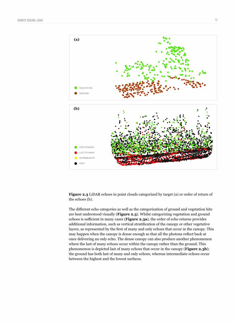
Figure 2.3 LiDAR echoes in point clouds categorized by target (a) or order of return of the echoes (b).

The different echo categories as well as the categorization of ground and vegetation hits are best understood visually (Figure 2.3). Whilst categorizing vegetation and ground echoes is sufficient in many cases (Figure 2.3a), the order of echo returns provides additional information, such as vertical stratification of the canopy or other vegetative layers, as represented by the first of many and only echoes that occur in the canopy. This may happen when the canopy is dense enough so that all the photons reflect back at once delivering an only echo. The dense canopy can also produce another phenomenon where the last of many echoes occur within the canopy rather than the ground. This phenomenon is depicted last of many echoes that occur in the canopy (Figure 2.3b); the ground has both last of many and only echoes, whereas intermediate echoes occur between the highest and the lowest surfaces.

REMOTE SENSING: LIDAR 14

The LIDAR sensor is positioned in an opening created in the underbelly of the airplane.

Image: © E.Sombié/WWF

Image: © E.Sombié/WWF

LiDAR unit inside the aircraft generates the

powerful laser pulses which comprise the

LiDAR measurements for lidar unit image

REMOTE SENSING: LIDAR 15

UNDERSTANDING THE DATA

3.1 Types of LiDARLiDAR data can come in two forms, discrete return and full waveform data. Whereas many of the principles covered in this guide apply to both types of data, this guide focuses exclusively on discrete return data because they are the most common publicly available datasets. In the collection phase of discrete return data, the system counts an echo only if the incoming echo exceeds a pre-defined threshold of intensity. In practice, this has the effect that echoes reflected from certain objects, for example a single tree branch, may not provide sufficient intensity to be recorded in discrete return data – discrete return data records information only from targets that yielded a strong enough return. This intensity threshold can be adjusted. In contrast, in full waveform data the whole waveform is practically digitized, regardless of intensity or strength. This guide focuses on discrete return data. For more information about full waveform data, refer to Mallet & Bretar (2009), Hollaus et al. (2014), Hovi (2015), or Hovi et al. (2016). Further, Sumnall et al. (2015) provide examples of estimating forest variables with both discrete-return and full waveform data.

3.2 Format and structureThe vast majority of publicly available LiDAR data is discrete return data and most commonly it is provided in LAS or LAZ (.las/.laz) format. The LAS format is a format used by the American Society of Photogrammetry and Remote Sensing (ASPRS). LiDAR data contain information on the echoes of emitted pulses. The most important information describing each pulse are categorized as X, Y, Z, I, N, R, C. X, Y and Z are the coordinates of the echo locations (the location where this echo came from, typically the coordinates are projected in the local coordinate system). I indicates the intensity or strength of the echo. N represents the number of returns (echoes) received from a single pulse and R indicates the order of these echoes, or the return number. For example, a combination of N = 2 and R = 1 indicates that two echoes were recorded from this pulse (N = 2) of which this record is the first (R = 1). It is common for echoes in public data to be classified into categories and the column C indicates these categories for this classification.

HIGHLIGHTS• LiDAR data can either be discrete or full waveform; discrete data represent the

majority of publicly available data

• LiDAR data consist of the 3D coordinates of the laser echo, the intensity of the echo, the number and order of echoes from a single laser pulse, and frequently a category of surface off which the echo reflected

ASPRS full description: www.asprs.org/a/society/committees/standards/LAS_1_4_r13.pdf.

REMOTE SENSING: LIDAR 16

Figure 3.1 LiDAR data in text format (.txt) from 9 echoes.

When LiDAR data are converted into text format (Figure 3.1) the first row contains column headings, and subsequent rows contain the X, Y, Z, I, N, R, C data for each received echo. According to this dataset, the first echo reflected off vegetation (C=3) whereas the last two echoes reflected off the ground (C=2). The first three echoes provide an illustrative example of the N and R categories. The value of N is 3 for all three echoes, indicating that they all originated from the same pulse. The values of R varies from 1 to 3, indicating that the first three rows hold information for the three echoes that were received from the emitted pulse. The rows that have a value of 1 for N and a value of 2 for C are ground hits, where the pulse hit ground without intersecting any vegetation or other objects in its path, hence producing a single echo. The last and second to last echoes also show a pattern. The third to last echo has a value of 2 for N, 1 for R, and 3 for C, indicating that two echoes were received from this pulse, of which this echo is the first one, and it reflected off vegetation. After the pulse encountered the vegetation and reflected some of the its photons, the remaining photons continued the journey before reflecting off the ground and yielded the last echo as indicated by the value of 2 for N, 2 for R, and 2 for C; of the two echoes received from this pulse, this, the last of them, reflected off the ground.

Close scrutiny of the data in Figure 4 suggests that some of the reflections from vegetation occurred at heights of more than 300 meters! Comparison of these Z values to those from ground reflections which are also greater than 300 meters provides an explanation for this seemingly spurious phenomenon. The Z coordinate in the data does not refer to the height above ground level, but needs to be scaled to reflect this. This core step is addressed in the next chapter.

X Y Z I N R C597847.589 7336016.990 329.020 1 3 1 3

597847.290 7336017.230 325.050 1 3 2 3

597846.979 7336017.490 320.780 1 3 3 1

597845.609 7336017.429 319.820 14 1 1 1

597842.969 7336017.230 319.330 18 1 1 2

597840.359 7336017.009 319.060 17 1 1 2

597838.520 7336016.200 328.500 8 1 1 1

597836.849 7336016.370 323.710 5 2 1 3

597836.469 7336016.660 318.960 0 2 2 2

REMOTE SENSING: LIDAR 17

DATA PROCESSING AND DELIVERABLES

VEGETATION ECHOS GROUND ECHOS DIGITAL ELEVATION MODEL (FROM GROUND ECHOS)

This chapter covers basic processing and analyses of LiDAR data without reference to any particular program. Chapter 7 introduces software that are commonly used to process and analyse LiDAR data. The data used here for illustrative purposes is publicly available low-pulse density data (~ 1 pulses/ m2) that has been processed (Figure 3.1). The figures in this section were produced from publicly available LiDAR data of the National Land Survey of Finland.

4.1 Aim of data processingIn order to calculate, for example, meaningful metrics of vegetation structure, the Z-coordinates in LiDAR point clouds need to be scaled to above ground level (agl). This can be achieved by first creating a terrain model from the ground echoes (Figure 3.1, C=2) and then using this terrain model to re-scale the echo heights. In practice, this is usually achieved by separating the ground echoes from the other echoes, and then interpolating a digital terrain model (DTM) from them (Figure 4.1).

HIGHLIGHTS• Translating raw LiDAR data into ecologically relevant datasets requires some data

processing, including scaling the height of echoes relative to ground level

• Common data products from LiDAR include digital terrain and canopy height models

• Although LiDAR data usually require significant processing before use, the raw data contain an incredible wealth of information, allowing the derivation of myriad relevant datasets

Figure 4.1 Vegetation echoes and ground echoes separated from a 25 meter wide circle, and a digital elevation model interpolated from the ground echoes.

DTMs are often rasters (e.g. in a .tiff format), where each cell´s (pixel of a raster image) value indicates its elevation. The next step involves subtracting this DTM value from the other (non-ground) echoes by identifying the DTM cell within which the LiDAR echo falls and subtracting the DTM cell´s Z value from the LiDAR echo Z value. What remains is the metric difference in Z between the cell (ground level) and the LiDAR echo, and this value represents the height of our LiDAR echo above ground level (Figure 4.2).

REMOTE SENSING: LIDAR 18

Figure 4.2 LiDAR echoes with their Z-coordinates scaled to above ground level height. The grey circle has a 25 meter radius and an elevation of 0 meters (ground level). The shading of the echoes symbolizes their height.

4.2 Common LiDAR data productsThe DTM discussed in the previous section is a basic LiDAR product. DTMs are the products that are most often of interest to National Land or Ordnance Surveys. The National Land Survey of Finland for example is producing a LiDAR-based DTM with two meter spatial resolution (one pixel is 2 x 2 meters) covering the entire country. This allows for highly accurate models of the terrain and elevation (Figure 4.3).

24

18

12

6

0

(a)

(b)

Figure 4.3 Digital terrain model in 2D (a) and a 3D visualization of a 2D DTM (b). The black shape in a is a river at an elevation of 230 meters above sea level. The whitest (highest) points in a are at approximately 340 meters above sea level.

REMOTE SENSING: LIDAR 19

The DTM of Figure 4.3a can then be used to derive additional data such as slope steepness, visibility from a certain location (viewshed), or aspect. For example, Figure 4.3b illustrates the steepness of the slope with green representing areas with low slopes (flat areas) and red representing areas with high slopes (steep areas). Although interesting and relatively easy to create in GIS software, their creation falls outside the scope of this guide.

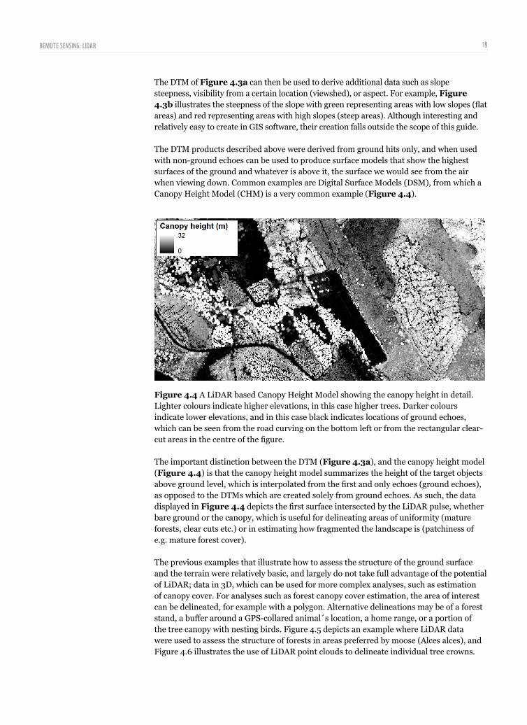
The DTM products described above were derived from ground hits only, and when used with non-ground echoes can be used to produce surface models that show the highest surfaces of the ground and whatever is above it, the surface we would see from the air when viewing down. Common examples are Digital Surface Models (DSM), from which a Canopy Height Model (CHM) is a very common example (Figure 4.4).

Figure 4.4 A LiDAR based Canopy Height Model showing the canopy height in detail. Lighter colours indicate higher elevations, in this case higher trees. Darker colours indicate lower elevations, and in this case black indicates locations of ground echoes, which can be seen from the road curving on the bottom left or from the rectangular clear-cut areas in the centre of the figure.

The important distinction between the DTM (Figure 4.3a), and the canopy height model (Figure 4.4) is that the canopy height model summarizes the height of the target objects above ground level, which is interpolated from the first and only echoes (ground echoes), as opposed to the DTMs which are created solely from ground echoes. As such, the data displayed in Figure 4.4 depicts the first surface intersected by the LiDAR pulse, whether bare ground or the canopy, which is useful for delineating areas of uniformity (mature forests, clear cuts etc.) or in estimating how fragmented the landscape is (patchiness of e.g. mature forest cover).

The previous examples that illustrate how to assess the structure of the ground surface and the terrain were relatively basic, and largely do not take full advantage of the potential of LiDAR; data in 3D, which can be used for more complex analyses, such as estimation of canopy cover. For analyses such as forest canopy cover estimation, the area of interest can be delineated, for example with a polygon. Alternative delineations may be of a forest stand, a buffer around a GPS-collared animal´s location, a home range, or a portion of the tree canopy with nesting birds. Figure 4.5 depicts an example where LiDAR data were used to assess the structure of forests in areas preferred by moose (Alces alces), and Figure 4.6 illustrates the use of LiDAR point clouds to delineate individual tree crowns.

REMOTE SENSING: LIDAR 20

Figure 4.5. Locations of GPS-collared moose (left) visualized inside LiDAR data. LiDAR data extracted and visualized in more detail around one of the locations (right). Figure adapted from Melin et al. 2014.

Figure 4.6. Tree crowns detected and delineated from LiDAR point cloud data. Figure adapted from Vauhkonen et al. 2014, 2016.

The purpose of the analyses depicted in the two figures is to use the 3D information to assess more complex structural features that are ecologically-relevant. In these cases, the relevant structural features were 3D variables suitable for forest height and vegetation structure modelling. As shown in these brief examples, LiDAR data are suitable for a diversity of analyses aimed at understanding environmental 3D structure.

The examples above provide only a cursory examination of the myriad potential applications of LiDAR, and the next chapter reviews in greater detail some additional applications of LiDAR such as mapping vegetation and forest resources, land cover analyses, bathymetry, wildlife habitat analysis, and discusses the types of variables useful for deriving the desired information from LiDAR data.

REMOTE SENSING: LIDAR 21

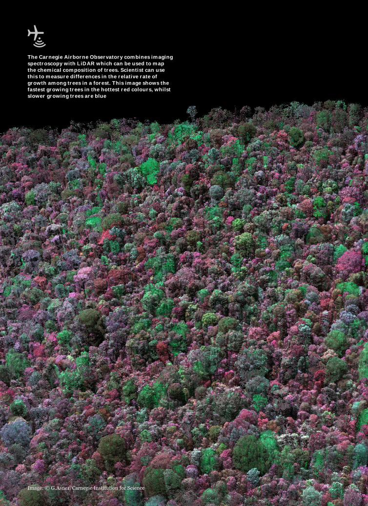
Image: © G.Asner/Carnegie Institution for Science

The Carnegie Airborne Observatory combines imaging

spectroscopy with LiDAR which can be used to map

the chemical composition of trees. Scientist can use

this to measure differences in the relative rate of

growth among trees in a forest. This image shows the

fastest growing trees in the hottest red colours, whilst

slower growing trees are blue

REMOTE SENSING: LIDAR 22

LIDAR APPLICATIONSHIGHLIGHTS• LiDAR has seen numerous applications across multiple disciplines, including

geography, geology, ecology, pedology, hydrology, conservation biology, and forestry

• For many species, vegetative structure is a critical component of habitat suitability, and LiDAR has been used to better understand wildlife-habitat relationships and even animal behaviour across multiple species and systems

• LiDAR can also be used to map land cover and land use, flood risk, bathymetry, and carbon storage

This chapter provides select examples of LiDAR’s use in applied and research contexts. Whereas this section seeks to provide a relatively broad image of how LiDAR data is used, the rapid growth of LiDAR and its diversity of uses makes a comprehensive yet useful summary nearly impossible. Interested readers should refer to the included references for more detailed examples.

5.1 Forestry, vegetation structureIn many countries LiDAR is already in operational use in the forestry sector, where it is used for forest inventory purposes. Variables that are commonly used in forestry applications include height and density percentiles of the vertical distribution of the LiDAR echoes calculated from the first and only echoes or from last echoes. Commonly these variables are named h5, h10,…, h100. However, if calculated with categorizing echoes then the prefix f_h80 or l_h80 is frequently used to refer to first or last echoes, respectively. For example, the variable h80 indicates the agl height below which 80% of all the echoes were received. For example, and h80 value of 21.3 indicates that 80% of the echoes received from this area came below the height of 21.3 meters. Other common variables are the mean, maximum and standard deviation of the echo heights.

Calculating the variables in forestry typically entails gridding the study area (or forest stands) and calculating the selected variable for each grid cell. For example, the echoes coming from inside a single grid cell are analysed separately from the other echoes, so the created variables will be cell-specific: e.g. the mean height of LiDAR echoes inside this cell, and then the desired variables for those echoes are calculated. Extending this to the entire study area produces maps of forest structure based on the LiDAR variables (Figure 5.1).

For a wide range of LIDAR applications, refer to: cao.carnegiescience.edu

REMOTE SENSING: LIDAR 23

Figure 5.1 A common example where LiDAR variables have been calculated for a forest stand that has been gridded into 16 x 16 meter grid cells. The final LiDAR variables have been then used to predict forest characteristics of interest within each grid cell, in this case volume of timber.

The application of LiDAR in forestry is far more diverse and widespread than covered here and outside the scope of this guide. Readers interested in learning more about the history and other uses of LiDAR in forestry should refer to Hudak et al. (2009), White et al. (2013), and Maltamo et al. (2014). As forests cover a broad range of different types, the use of LiDAR is consequently very different between e.g. boreal coniferous forest or a tropical rain forest. The main issue, no matter what the environment, is to reliably detect the ground, without which the echo heights do not have a practical meaning. Nonetheless, LiDAR has been applied in many different forest environments.

The practical use of LiDAR was first pioneered in boreal forests due to their “easy” structure. Unlike rain forests they are not composed of dense multiple layers so the pulses have a higher probability of reaching the ground, which makes the data itself more accurate because the ground surface can be reliably detected and modelled with high accuracy. By contrast, the dense structure of tropical rain forests posed a major obstacle to LiDAR use. However, as the devices improved it became possible to use LiDAR in more challenging environments such as tropical forests. Examples of use of LiDAR in tropical forests are provided by Asner et al. (2012) and Leitold et al. (2015), whilst Hansen et al. (2015) provide examples of the challenges proposed by tropical forest structure and how to overcome them.

5.2 Analysis of land cover, topography and hydrologyIn addition to its utility for mapping vegetative structure, LiDAR has also been employed to assess landcover, topography and hydrology. Kiss et al. (2015, 2016) used LiDAR to assess forest road conditions. In their studies, the analysis was conducted with LiDAR-based DTMs, from which the topography of the road and the surrounding ditches and terrain was assessed in great detail. The key determinant of the road quality was hydrology and the flow of water, which they were able to assess based on the 3D characteristics of the road.

In general, LiDAR-based assessments of soil moisture content and topographic wetness or flow of water have been studied in detail. For soil moisture content, see Gillin et al. (2015) or Tenebaum et al. (2006). For examples of topographic wetness index (TWI) calculations based on LiDAR, see Buchanan et al. (2014). For more applied cases, see the LiDAR-based mapping of flood risk areas by Bales et al. (2007). Also, in a recent work, Pippuri et al. (2016) showed that LiDAR data can be used to classify land cover and land use in boreal forests.

0.00 - 46.42

46.43 - 115.83

115.84 - 182.19

182.20 - 247.73

247.74 - 411.74

CANOPY HEIGHT (METRES) LiDAR BASED PREDICTIONS VOLUME (m3/ha)FOREST STAND BORDERS

32

0

REMOTE SENSING: LIDAR 24

5.3 Ecological applications That vegetation structure is a primary determinant of habitat quality was first noted in the seminal work of MacArthur & MacArthur (1961). This concept is very practical; the structure and arrangement of vegetation is what ultimately defines the distribution and abundance of critical habitat components such as food, nesting sites (in the canopy or on the ground), thermal shelters, cover against predation, and camouflage. LiDAR provides data that can be used to estimate all of these and other variables with unprecedented precision at the landscape-level. A review of this concept is provided in Vierling et al. (2008).

The application of LiDAR to estimating habitat-related variables is summarized in the following sections. For organizational purposes, this section has been divided into variable estimation for volant and canopy species, terrestrial species, biodiversity mapping, mapping of important habitats (hot-spots), and the estimation of attributes that are often linked to global conditions of forests and vegetation such as Leaf Area Index (LAI) and canopy cover. As with the other sections, it is not possible to cover all the studies or aspects and readers are encouraged to reference publications cited therein for additional details.

5.3.1 Volant and canopy speciesBirds were the species with which the connection between LiDAR and wildlife ecology was first published in the work of Hill et al. (2004). Since that initial work, multiple other researchers have found LiDAR useful for assessing habitat of canopy-dependent, as well as ground-nesting, birds (Graf et al. 2009; Martinuzzi et al. 2009; Goetz et al. 2010; Hill & Hinsley 2015, Zellweiger et al. 2013, Zellweiger et al. 2016; and Melin et al. 2016). Arboreal mammals living in trees have also been a topic of LiDAR-based studies that have revealed patterns in habitat use preference in relation to canopy structure. Species included in these analyses include bats (Froidevaux et al. 2016), primates (Palminteri et al. 2012), and squirrels (Flaherty et al. 2014).

The methods applied to research questions have varied between the studies. Palminteri et al. (2012) focused on assessing the home-ranges and thereby the occurrence of their target species based on first studying the canopy structure (from LiDAR) in the areas mostly used by the target species. Melin et al. (2016) extracted LiDAR data from presence and absence locations of boreal grouse broods and thereby estimated what are the structural features of forests that mostly define a good grouse brood habitat. In the latter study, the LiDAR data was integrated with field inventory data, which allowed to spatially define the areas of presence and absence.

5.3.2 Terrestrial species Examination of forest structure relative to the habitat use of terrestrial species is linked to the abundance of important attributes such as availability of food or shelter, which presumably provides greater insights than do more typical metrics such as cover type. Recent target species for these analyses have included ungulates (Coops et al. 2010; Melin 2015, Lone et al. 2014), bears (Wulder et al. 2008) and lions (Davies et al. 2016); as with birds, the methods have varied between the studies. Lone et al. (2014) gridded the study area into 50 x 50 meter cells and extracted LiDAR data from each of the cells. Next, they created LiDAR metrics that were used to predict the availability of browse biomass for moose in each of the cells, thus defining the suitability of this cell for moose. Davies et al. (2016) first identified the potential kill sites of lions and then extracted LiDAR data from the area of these sites to assess the structure of their vegetation.

REMOTE SENSING: LIDAR 25

5.3.3 Mapping suitable habitat Many of the studies listed above have integrated LiDAR with locations from tagged or collared animals to examine habitat structure relative to use. LiDAR has also been used to locate features of habitats or the canopy that are known to be required by a specific species, which then allows the modelling of the suitability of a habitat patch or area in the landscape and the distribution of suitable habitat. For example, coarse woody debris and snags are important components of suitable habitat for many species and LiDAR has been used to map their distribution. Pesonen (2010) used LiDAR data to successfully assess the presence and abundance of coarse woody debris, the presence of which is a key determinant of boreal forest biodiversity. Martinuzzi et al. (2009) improved habitat suitability estimates for four bird species by the inclusion of LiDAR data, which was due to it being able to catch the presence of snags and features of vegetation structure deemed important for the species in question. Back in the boreal zone, Vehmas (2010) used LiDAR data to map old-growth coniferous stands and stands with high herbaceous diversity.

5.3.4 Estimating canopy cover and leaf area index Variables such as Canopy Cover (CC) and Leaf Area Index, (LAI) are frequently used as proxies for classifying forests and assessing their condition and LiDAR has proven to be a highly accurate tool for these tasks. Korhonen (2011) and Korhonen et al. (2011) provide examples of assessing LAI and CC from LiDAR, and Vehmas et al. (2011) illustrate how to detect canopy gaps and understory in boreal conditions whilst Hill & Broughton (2009) mapped the understory of deciduous forests of England using leaf-on and leaf-off LiDAR data.

5.3.5 Detecting forest changeForest and vegetation structural changes occur continuously for a host of reasons, including natural succession, weather, damages or harvesting and logging. LiDAR data has been successfully used to identify the severity of extent of these kinds of changes. Examples include change resulting from snow damage (Vastaranta et al. 2012), insect damage (Coops et al. 2009; Solberg et al. 2006; Vastaranta et al. 2013), moose browsing damage (Melin et al. 2016), and natural succession (McRoberts et al. 2014). It is naturally obvious that LiDAR is particularly well suited to detect man-induced changes such as harvesting or clear-cutting (Figure 5.2).

Figure 5.2 Changes in the New Forest National Park (England, UK) visualized from LiDAR data collected in 2009 (a) and 2015 (b). White colour indicates higher vegetation; taller trees.

REMOTE SENSING: LIDAR 26

As seen in Figure 5.2, the change is detectable in the CHM raster image as well. There is no need for detailed point cloud analysis if the aim is to document that a change has taken place. The change in the lower left corner is regrowth based on the appearance of small grey trees growing on image b. In the top right corner, we see both the removal of trees and the growth of those that remained (the trees appear whiter in the image b).

5.4 Forest biomass mappingREDD+ (Reducing Emissions from Deforestation and Degradation) is a framework designed to incentivise the protection and retention of carbon contained in forests. LiDAR has been increasingly used for mapping above-ground forest biomass, as the ability to penetrate the canopy and determine three-dimensional structure at scale is useful for estimating forest carbon stock (Lefksy et al. 2002). To estimate biomass, LiDAR data are calibrated with information from field inventory plots, which may include data on diameter at breast height (DBH), basal area, or wood density. These metrics, along with precise measurements of forest canopy height and ground surface from LiDAR are used to develop appropriate biomass models (Asner et al. 2012, Kotivuori et al. 2016) which accurately estimate carbon stock nearly as well as field plots (Mascaro et al. 2011), while reducing the need for extensive ground inventories (Ferraz et al. 2016). Use of these techniques enables national-scale mapping of biomass (Asner et al. 2013) and can be used to monitor biomass over time (Meyer et al. 2013). For additional examples of LiDAR being applied for REDD+ analyses refer to Joshi et al. (2014), Leitold et al. (2015), Tokola (2015), Ene et al. (2016), and Kauranne et al. (2017).

5.4 BathymetryThe purpose of bathymetric LiDAR is to provide detailed information on water depth and underwater barriers for navigation of water bodies, and to date bathymetric scans have been completed for the shores of Alaska and the Caribbean. Bathymetric LiDAR differs from terrestrial LiDAR in one important way. Because bathymetric LiDAR aims to map the structure of the terrain below the water surface it must employ a laser that emits pulses that differ in wavelength to those emitted by terrestrial LiDAR devices; the wavelengths of pulses emitted by terrestrial LiDAR devices are unable to penetrate the surface of the water, and rapidly attenuate near the surface. Devices meant for bathymetric purposes use lasers operating at shorter wavelengths, which penetrate the water and thus give echoes from the lake or sea bottom, enabling one to map depth and accurately depict the 3D terrain of the ocean/lake floor. This is very similar to the DTM in Figure 4.3b. The depth the laser can reach is dependent on the clarity of the water; the clearer the water, the deeper the pulse’s reach. Bathymetric LiDAR data, including its application in coral reef conservation, can be found in Brock et al. (2004), Pittman et al. (2009), Pe´eri et al. (2011),

For additional details about biomass mapping, please refer to:

carbon.jpl.nasa.gov

REMOTE SENSING: LIDAR 27

Image: © S. Popescu

Terrestrial lidar scan of oak trees during leaf-off season

REMOTE SENSING: LIDAR 28

LIDAR HORIZONSHIGHLIGHTS• Future LiDAR datasets will likely include multispectral properties and improved

spatial and temporal coverage and resolutions

• These advances will increasingly allow mapping of annual or more frequent changes in the distribution and abundance of individual species at the global scale

This chapter briefly discusses new and upcoming applications of LiDAR for surveying terrestrial ecosystems. For a recent in-depth review of LIDAR horizons, see Eitel et al. (2016).

6.1 Multi-wavelength (or multispectral) LiDAR Multispectral LiDAR is a technique that is currently receiving intense interest from many researchers and it is rapidly developing, particularly in forestry. The core principle is that the use of multi-wavelength LiDAR can discriminate more efficiently among the types of surfaces from which the echoes reflect. For example, use of multispectral LiDAR can distinguish among coniferous and deciduous trees, bare and vegetated ground, and in some cases individual tree species. These discriminations are invaluable as they can result in species-specific estimates of vegetative structure, which in turn yields more accurate estimates of the species-specific variables of forest structure, stock, and volume. Furthermore, the ability of multispectral LiDAR to identify individual species will assist in locating endangered tree species. The potential application of this technique to wildlife ecology is also promising, because of its complementarity to structure; having accurate estimates of species-specific vegetative structure would improve models of habitat suitability and identification of vital habitat patches for specialist species.

Multispectral LiDAR is able to distinguish among the different surfaces because it utilizes lasers employing wavelengths that are able to differentiate chlorophyll levels (Nevalainen et al. 2014). Because plants possess chlorophyll and its concentration differs among species, multispectral LiDAR is able to discriminate between the presence and absence of chlorophyll (for example between bare ground and vegetation) and in some cases among species that differ in chlorophyll content, for example between coniferous and deciduous species. We are yet to see the full potential of this data to the wildlife research community.

6.2 Spaceborne systemsLiDAR sensors have also been placed on board satellites, and these provide global LiDAR data, but at coarser resolutions. For instance, the NASAs GEDI LiDAR has a resolution of 25 meters (the width of the pulse as it hits the ground and the pulses come between ~60 meters. These datasets are freely available and are useful for large-scale estimates of ecosystem structure, but they cannot provide information about what is happening within the 25 meter area of the pulse. The limitation of this coarse resolution was documented by Vierling et al. (2013) who tested the utility of both airborne and spaceborne (GLAS) LiDAR data in modelling woodpecker habitat occupancy. They concluded that the coarse resolution of the spaceborne data was unable to capture habitat information at a sufficiently fine scale. Despite these limitations, spaceborne LiDAR data remain valuable for large-scale, low resolution analyses, such as for the GLAS LiDAR based 500 meter resolution canopy height map of the Amazon (Sawada et al. 2015) and global maps of biomass (Baccini et al. 2012). Examples of more research conducted with the spaceborne systems as well as comparisons of spaceborne systems to ALS systems are provided in Bergen et al. (2009), Popescua et al. (2011), Suna et al. (2008) and Tanga et al. (2014).

attic.gsfc.nasa.gov/glas/

nsidc.org/data/docs/daac/glas_icesat_l1_l2_global_altimetry.gd.html#data_description

More information on the spaceborne systems can be found here:

NASA GEDI:

NASA GLAS:

eospso.nasa.gov/missions/global-ecosystem-dynamics-investigation-LiDAR

science.nasa.gov/missions/gedi

REMOTE SENSING: LIDAR 29

This section is not intended to be comprehensive or prescriptive, as the programs to process LiDAR are numerous and increasing rapidly in accordance with the evolving field and user needs. In addition, those with programming skills and the right knowledge may prefer to write their own programs for their own needs. Therefore, this section briefly introduces a few of the more commonly used software including GIS and remote sensing programs.

Detailed information on each tool is not given, but links (current at the time of writing) to the software guidelines are provided. Some programs (e.g. LAS Tools, Fusion and Opals) have been specifically designed for processing and analysing LiDAR, whereas others (e.g. QuantumGIS, ArcGIS, ENVI) are well-known GIS and remote sensing software which also have LiDAR functionality.

LIDAR SOFTWARE

REMOTE SENSING: LIDAR 30

Software Website Description

Software Website Description

LAS Tools rapidlasso.com/lastools The data in Figure 3.1 were converted from LAZ to text with LA2TXT software by Martin Isenburg. LAS Tools offer every tool needed from raw data processing to analysis and variable extraction. LAS Tools runs on command line, but also offers a graphical user interface (GUI) for those not comfortable with command lines and batch scripting. Every tool (e.g. las2DTM or las2txt) comes with its own README file, which tells in principle what the tool is used for and how it is used (inputs, outputs, parameters etc.). For an example, see the README on las2DTM: www.cs.unc.edu/~isenburg/lastools/download/las2DTM_README.txt.

Fusion forsys.cfr.washington.edu/fusion.html

Fusion is a free program designed also for efficient LiDAR data processing and analysis. Overviews of the LiDAR processing tools and principles of Fusion as well as tutorials on these matters are provided at:

www.fs.fed.us/eng/rsac/LiDAR_training www.dataone.org/software-tools/fusion-LiDAR-software

Opals geo.tuwien.ac.at/opals/html/index.html

Opals (Orientation and Processing of Airborne Laser Scanning data), made by researchers at Vienna University of Technology, provides a full chain of tools from raw data processing up until variable extraction and different applications. The program as well as DTMonstrations on how to get started using the software are available at the website.

Quantum GIS (QGIS)

www.qgis.org Quantum GIS, or QGIS, is one of the most popular open-source GIS programs. QGIS processes LiDAR data via the LAS Tools software that can be installed as its own toolbox. For instructions on how to install the software, refer to: rapidlasso.com/2013/09/29/how-to-install-lastools-toolbox-in-qgis or docs.qgis.org/2.2/en/docs/training_manual/forestry/basic_LiDAR.html

ENVI www.harrisgeospatial.com/ProductsandTechnology/Software/ENVI.aspx

In addition to its utility for processing and analysing LiDAR datasets, ENVI has a range of functionality for GIS and remote sensing analyses. Information about the use of ENVI to process LiDAR data can be found at:exelis.http.internapcdn.net/exelis/pdfs/2-13_ENVILiDAR_Brochure_LoRes.pdf

www.exelisvis.co.uk/ProductsServices/ENVIProducts/ENVILiDAR.aspx

ENVI also has a designated LiDAR plug-in developed by Idaho State University. This plug-in (BCAL LiDAR) is meant purely for LiDAR processing and is available at:bcal.boisestate.edu/tools/LiDAR

ArcGIS www.esri.com/arcgis/about-arcgis

ESRI’s ArcGIS family is one of the most widely used GIS software. It also has its own tools for handling, processing, and analysing LiDAR datasets. Some guidelines on how to use the tools are available at:desktop.arcgis.com/en/arcmap/10.3/manage-data/las-dataset/a-quick-tour-of-LiDAR-in-arcgis.htm

desktop.arcgis.com/en/arcmap/10.3/manage-data/las-dataset/using-LiDAR-in-arcgis.htm

www.esri.com/esri-news/arcuser/summer-2013/5-ways-to-use-LiDAR-more-efficiently

ERDAS IMAGINE

www.hexagongeospatial.com/products/power-portfolio/erdas-imagine

ERDAS IMAGINE is a widely used remote sensing software that also offers tools for LiDAR. Information and examples are available at:igic.org/archives-training/pres/conf/2012/ERDAS_IMAGINE_for_LiDAR_IGIC_Workshop.pdf

FugroViewer www.fugroviewer.com Is a fast and easy-to-use tool for visualizing LiDAR data

Table 3. A brief description and download links to select software for processing LiDAR data.

REMOTE SENSING: LIDAR 31

Image: © G. Asner/Carnegie Institution for Science

This map of estimated above ground forest carbon

density in Peru was developed using airborne

LIDAR, satellite imagery, and field data in 2014 by

the Carnegie Institution for Science at Stanford

University, Wake Forest University, and Peru’s

Ministry of Environment

REMOTE SENSING: LIDAR 32

LiDAR data are being collected by numerous national land survey agencies, research institutions, and forestry agencies and companies. In many cases these data are freely available, but not always, as some private companies collect the data in order to sell it to end users. This section aims to provide a list of the countries that have collected LiDAR data or are planning to do so, and links to the agencies or organizations through which these data can be acquired.

The available data formats, different products (e.g. DTMs) are not listed in this section because these details are provided by the data distributor. Given the ephemeral nature of the internet some links may not remain functional but readers should be able to locate the data sets based on the information contained herein.

When a country is not mentioned in the list it means that no information was available (or was not found) from the status of their LiDAR collection plans. Searches were done from the internet and through direct consultation with geospatial agencies and national land surveys. The URL in the table leads either directly to the data download service or into a web-page/document describing the data acquisition process. The list has both free LiDAR data as well as data for sale.

Country Website

Amazonia infoamazonia.org/data

Antarctica usarc.usgs.gov/LiDAR_dload.shtml

Australia www.ga.gov.au/scientific-topics/national-location-information/digital-elevation-data

Australia data.auscover.org.au

Austria www.data.gv.at/katalog/dataset/a0c7c877-7abb-46f8-b2fb-0d5578ceee64

Belgium www.ngi.be/FR/FR1-5-5.shtm

Brazil www.ibge.gov.br/english/geociencias/default_prod.shtm#REC_NAT

Canada airborneimaginginc.com/LiDAR-data-library-downloads

Croatia geoportal.nipp.hr/en

Cyprus www.geoportal.gov.cy

Denmark download.kortforsyningen.dk

Ecuador www.sigtierras.gob.ec

Estonia geoportaal.maaamet.ee/eng/Maps-and-Data/Topographic-Data/Elevation-data-p308.html

Estonia geoportaal.maaamet.ee/eng/Ordering-Data-p301.html

Finland tiedostopalvelu.maanmittauslaitos.fi/tp/kartta?lang=en

France ids.equipex-geosud.fr/web/guest/donnees-LiDAR-satellitaire

Germany www.geodatenzentrum.de/geodaten/gdz_rahmen.gdz_div?gdz_spr=eng&gdz_akt_zeile=2&gdz_anz_zeile=4&gdz_user_id=0

Germany www.geodatenzentrum.de/geodaten/gdz_rahmen.gdz_div?gdz_spr=eng&gdz_akt_zeile=5&gdz_anz_zeile=0&gdz_user_id=0

DATA ACQUISITION AND AVAILABILITY

REMOTE SENSING: LIDAR 33

Greece www.ktimatologio.gr

Greece www.gys.gr

Hungary www.geoshop.hu/index.php?module=Products&cmd=selectProducts

Iceland www.lmi.is/en/stafraen-gogn

Iran www.ncc.org.ir/HomePage.aspx?lang=en-US&site=NCCPortal&tabid=1

Iran www.ngdir.ir

Ireland www.osi.ie/products/bluesky-aerial-imagery-LiDAR

Japan www.gsi.go.jp/ENGLISH/page_e30031.html

Japan www-LiDAR.nies.go.jp

Latvia kartes.lgia.gov.lv/karte/?lang=en

Latvia map.lgia.gov.lv/index.php?lang=2&cPath=4_5&txt_id=126

Malta information.resources@pa.org.mt

Malta www.seismalta.org.mt

Mexico www.inegi.org.mx/geo/contenidos/geografia/default.aspx

Netherlands www.ahn.nl/pagina/open-data.html

Netherlands www.swartvast.nl/rapporten/AHN_as_massive_point_cloud_data_LMTh_Swart.pdf

New Zealand www.mfe.govt.nz/more/data/available-datasets/forest-soil-and-LiDAR-data

New Zealand koordinates.com/publisher/linz/data/category/contours-terrain/LiDAR-elevation-points

Norway 159.162.103.4/geovekst/georef.jsp?fylke=00&komm=0000&georef=Laser&Submit1=G%E5+til+kommune

Norway www.kartverket.no/Kart/Laserskanning

Poland codgik.gov.pl

Portugal mapas.dgterritorio.pt/LiDAR

Serbia Republic Geodetic Authority - tik@rgz.gov.rs

Slovenia gis.arso.gov.si/evode/profile.aspx?id=atlas_voda_LiDAR@Arso&culture=en-US

Spain centrodedescargas.cnig.es/CentroDescargas/catalogo.do#selectedSerie

Sweden www.lantmateriet.se/globalassets/kartor-och-geografisk-information/hojddata/produktbeskrivningar/eng/LiDAR_data.pdf

Switzerland www.swisstopo.admin.ch/internet/swisstopo/en/home/products.html

Thailand www.gistda.or.th/main

United Kingdom www.geostore.com/environment-agency/survey.html#/survey

USA lta.cr.usgs.gov/LiDAR_digitalelevation

Table 3. Sources for LiDAR data or related products.

Country Website

REMOTE SENSING: LIDAR 34

LiDAR is not a remote sensing panacea, and in many cases will not be necessary or even appropriate. Before deciding to put resources into LiDAR data acquisition, processing, and analysis, it is critical to consider the advantages and disadvantages of the method.

One potential alternative to LiDAR is photogrammetry, which uses stereo imagery and a technique called image matching to map and measure surfaces. Indeed, the high cost of LiDAR will make it inaccessible in some cases, and photogrammetry data are frequently less expensive to collect and depending on the need may be entirely suitable for mapping soil or coastal erosion (Heng et al. 2010). However, whilst photogrammetry can be accurate, lidar remains more accurate when it comes to 3D structure. This is because as photogrammetry relies on reflected sunlight, it cannot see beneath the top-most surface of the forest canopy and therefore lacks data on subsurface/subcanopy structure (Tanhuanpää et al. 2016; Melin et al. 2017), although there have been some promising results in forest inventories (Bohlin et al. 2012; Kukkonen et al. 2017; Puliti et al. 2016; Puliti et al. 2017).

9.1 LiDAR weaknesses in briefLimited spatial and temporal availability. Freely available LiDAR datasets are available for a small fraction of the world, and are frequently limited to data collected at a single point in time.

High cost of collection of LiDAR data. LiDAR costs decrease per unit area as the total area surveyed increases, but can be substantial, and depend on the cost of fuel, pilots, airplane rental, all of which depend on geography and weather. There are several large international companies who do LiDAR data collection and will provide quotes1.

Technically complex processing, analysing and interpretations. LiDAR data processing is time-consuming and technically challenging, particularly for the unexperienced, and depending on the task may require expertise in GIS and remote sensing to use and interpret properly.

Lack of multispectral information. That LiDAR currently largely lacks multispectral data limits its utility to non-spectral analyses.

LiDAR cannot penetrate thick canopies. For instance, dense tropical forests are problematic due to lack of ground hits.

9.2 LiDAR strengths in briefMost accurate 3D information. LiDAR provides the most accurate data on 3D structure of any remote sensing technique, particularly when it comes to dense vegetation, with low-pulse density LiDAR typically exhibiting sub-meter accuracy.

Versatile data. LiDAR data can be used to produce digital models of terrain and canopy and customized for myriad needs to suit the research questions at hand.

High complementarity with remotely sensed imagery. LiDAR provides highly complementary data that can be used in conjunction with satellite and aerial imagery to gain insights that neither imagery nor LiDAR can reach alone (Asner et al. 2008; Packalén 2009; Cho et al. 2012; Melin et al. 2017).

LIDAR STRENGTHS AND WEAKNESSES

Companies:

airborneLiDARmapping.com

www.blomasa.com

www.teledyneoptech.com

www.aamgroup.com/services-and-technology/aerial-survey

airborneimaginginc.com/airborne-imaging-LiDAR-services/airborne-LiDAR

REMOTE SENSING: LIDAR 35

9.3 Summary of strengths and weaknessesMultispectral information is not present in standard LiDAR data. Aerial and satellite images provide information on the target´s reflectance at different wavelengths and so they can be used to detect different species or phenological stages of vegetation, but absent additional information LiDAR can be used only to assess the structure (Figure 9.1):

Figure 9.1 LiDAR-based canopy height model (CHM) and a false-colour infrared aerial image from the same location. Although the CHM provides information on tree height, it does not contain information on tree species, whereas the aerial image does. Here deciduous species are shown in red and coniferous as dark green.

The structural information from LiDAR and the spectral data from aerial or satellite imagery can be integrated to model species-specific vegetative structure (Figure 9.1), a method applied by Packalén (2009). Although classification of tree species from the geometry of LiDAR point clouds has been done (Vauhkonen 2010), publicly available data are generally not of sufficient resolution to do so. As such, although sufficiently high resolution LiDAR data are capable of identifying tree species under some circumstances, LiDAR alone is not commonly used to identify species; this can be overcome by integrating it with spectral data from another source such as aerial or satellite imagery.

A clear advantage of LIDAR is that it is stable and consistent - it can produce productssuch as DTMs which are comparable and hence can be used across time and space (Hill &Hinsley 2015; Vierling et al. 2014). Furthermore a stable and accurate DTM enables detailed monitoring of the vegetation above the ground surface.

REMOTE SENSING: LIDAR 36

Asner, G.P., Knapp, D.E., Kennedy-Bowdoin, T., Jones, M.O., Martin, R.E., Boardman, J. & Hughes, R.F. (2008). Invasive species detection in Hawaiin rainforests using airborne imaging spectroscopy and LiDAR. Remote Sens. Environ., 112, 1942-1955.

Asner, G.P., Mascaro, J., Muller-Landau, H.C., Vieilledent, G., Vaudry, R., Rasamoelina, M., Hall, J.S. & van Breugel, M. (2012). A universal airborne LiDAR approach for tropical forest carbon mapping. Oecologia, 168, 1147-1160.

Asner, G.P., Mascaro, J., Anderson, C., Knapp, D.E., Martin, R.E., Kennedy-Bowdoin, T., van Breugel, M., Davies, S., Hall, J.S., Muller-Landau, H.C., Potvin, C., Sousa, W., Wright, J. & Bermingham, E. (2013). High-fidelity national carbon mapping for resource management and REDD+. Carbon Balance and Management, 8:7.

Baccini, A., Goetz, S.J., Walker, W.S., Laporte, N.T., Sun, M., Sulla-Menashe, D., Hackler, J., Beck, P.S.A., Dubayah, R., Friedl, M.A., Samanta, S. & Houghton, R.A. (2012). Estimated carbon dioxide emissions from tropical deforestation improved by carbon-density maps. Nat. Clim. Change, 2, 182-185.

Bales, J.D., Wagner, C.R., Tighe, K.C. & Terziotti, S. (2007). LiDAR-derived flood-inundation maps for real-time flood-mapping applications, Tar River basin, North Carolina. U.S. Geological Survey Scientific Investigations Report 2007–5032, 42 p.

Bergen, K.M., Goetz, S.J., Dubayah, R.O., Henebry, G.M., Hunsaker, C.T., Imhoff, M.L., Nelson, R.F., Parker, G.G. & Radelof, V.C. (2009). Remote Sensing of vegetation 3-D structure for biodiversity and habitat: review and implications for LiDAR and radar spaceborne missions. J. Geophys. Res., 114.

Bohlin, J., Wallerman, J. & Fransson, J.E.S. (2012). Forest variable estimation using photogrammetric matching of digital aerial images in combination with a high-resolution DEM. Scand. J. Forest Res., 27, 692-699.

Brock, J.C., Wright, C.W., Clayton, T.D. & Nayegandhi, A. (2004). LiDAR optical rugosity of coral reefs in Biscayne National Park, Florida. Coral Reefs, 23, 48-59.

Buchanan, B.P., Fleming, M., Schneider, R.L., Richards, B.K., Archibald, J., Qiu, Z. & Walter, M.T. (2014). Evaluating topographic wetness indices across central New York agricultural landscapes. Hydrol. Earth Syst. Sci., 18, 3279-3299.

Cho, M.A., Mathieu, R., Asner, G.P., Naidoo, L., van Aardt, J., Ramoelo, A., Debba, P., Wessels, K., Main, R., Smit, I.P.J. & Erasmus, B. (2012). Mapping tree species composition in South African savannas using an integrated airborne spectral and LiDAR system. Remote Sens. Environ.,125, 214-226.

Coops, N.C., Wulder, M.A., Culvenor, D.S. & St-Onge, B. (2004). Comparison of forest attributes extracted from fine spectral resolution multispectral and lidar data. Can. J. Remote Sens., 30, 855-866.

Coops, N.C., Varhola, A., Bater, C.W., Teti, P., Boon, S., Goodwin, N. & Weiler, M. (2009). Assessing differences in tree and stand structure following beetle infestation using LiDAR data. Can. J. Remote Sens., 35, 497-508.

Coops, N.C., Duffe, J. & Koot, C. (2010). Assessing the utility of LiDAR remote sensing technology to identify mule deer winter habitat. Can. J. Remote Sens.,36, 81–88.

Davies, A.B., Tambling C.J., Kerley, G.I.H & Asner, G.P. (2016). Effects of Vegetation Structure on the location of lion kill sites in African thicket. PLoS One, 11, e0149098.

Eitel, J., Höfle, B., Vierling, L.A., Abellán, A., Asner, G.P., Deems, J.S., Glennie, C.L., Joerg, P.C., LeWinter, A.L. & Magney, T.S. (2016). Beyond 3-D: The new spectrum of LiDAR applications for earth and ecological sciences. Remote Sens. Environ., 186, 372-392.

Ferraz, A., Saatchi, S., Mallet, C., Jacquemoud, S., Gonçalves, G., Silva, C.A., Soares, P., Tomé, M. & Pereira, L. (2016). Airborne LiDAR Estimation of Aboveground Forest Biomass in the Absence of Field Inventory Remote Sensing. Remote Sens., 8, 653.

Flaherty, S., Lurz, P. & Patenaude, G. (2014). Use of LiDAR in the conservation management of the endangered red squirrel (Sciurus vulgaris L.). J. Appl. Remote Sens., 8, 423-427.

Froidevaux, J.S.P., Zellweger, F., Bollman, K., Jones, G. & Obrist, M.K. (2016). From field surveys to LiDAR: Shining a light on how bats respond to forest structure. Remote Sens. Environ., 175, 242–250.

BIBLIOGRAPHY

REMOTE SENSING: LIDAR 37

Gillin, C.P., Bailey, S.W., McGuire K.J. & Prisley, S.P. (2015). Evaluation of LiDAR-derived DRMs through Terrain Analysis and Field Comparison. Photogramm. Eng. Rem. S., 81, 387-396.

Goetz, S.J., Steinberg, D., Betts, M.G., Holmes, R.T., Doran, P.J., Dubayah, R. & Hofton, M. (2010). LiDAR remote sensing variables predict breeding habitat of a Neotropical migrant bird. Ecology, 91, 1569- 1576.

Graf, R. F., Mathys, L. & Bollmann, K. (2009). Habitat assessment for forest dwelling species using LiDAR remote sensing: Capercaillie in the Alps. Forest Ecol. Manag., 257, 160-167.

Hansen, E.H., Gobakken, T., Bollandsås, O.M., Zahabu, E. & Næsset, E. (2015). Modeling aboveground biomass in dense tropical submontane rainforest using airborne laser scanner data. Remote Sens., 7, 788-807.

Heng, B.C.P, Chandler, J.H. & Armstrong, A. (2010). Applying close range digital photogrammetry in soil erosion studies. The Photogrammetric Record, 25, 240-265.

Hill, R.A., Hinsley, S.A., Gaveau, D.L.A. & Bellamy, P.E. (2004). Predicting habitat quality for great tits (Parus major) with airborne laser scanning data. Int. J. Remote Sens., 25, 4851-4855.

Hill, R.A. & Broughton, R.K. (2009). Mapping the understorey of deciduous woodland from leaf-on and leaf-off airborne LiDAR data: A case study in lowland Britain. ISPRS J. Photogramm., 64, 223-233.

Hill, R.A & Hinsley, S.A. (2015). Airborne LiDAR for woodland habitat quality monitoring: exploring the significance of LiDAR data characteristics when modelling organism-habitat relationships. Remote Sens., 7, 3446-3466.

Höfle, B. & Rutzinger, M. (2011). Topographic airborne LiDAR in geomorphology: a technological perspective. Z. Geomorphol., 55, 1-29.

Hollaus, M., Mücke, W., Roncat, A., Pfeifer, N. & Briese, C. (2014). Full-waveform airborne laser scanning systems and their possibilities in forest applications. In: Forestry applications of airborne laser scanning – concepts and case studies. Springer Netherlands, Dordrecht, p. 43-62.

Hovi, A. (2015). Towards an enhanced understanding of airborne LiDAR measurements of forest vegetation. PhD dissertation, University of Helsinki.

Hovi, A., Korhonen, L., Vauhkonen, J. & Korpela I. (2016). LiDAR waveform features for tree species classification and their sensitivity to tree- and acquisition related parameters. Remote Sens. Environ., 173, 224-237.

Hudak, A.T., Evans, J.C & Smith, A.M.S. (2009). LiDAR utility for natural resource managers. Remote Sens., 1, 934-951.

Kiss, K., Malinen, J. & Tokola, T. (2015). Forest road quality control using ALS data. Can. J. Forest Res., 45, 1636-1642.

Kiss, K., Malinen, J. & Tokola, T. (2016). Comparison of high and low density airborne LiDAR data for forest road quality assessment. ISPRS Annals of the Photogrammetry, Remote Sensing and Spatial Information Sciences, Volume III-8, 167-172.

Korhonen, L. (2011). Estimation of boreal forest canopy cover with ground measurements, statistical models and remote sensing. PhD dissertation. University of Helsinki.

Korhonen, L., Korpela, I., Heiskanen, J. & Maltamo, M. (2011). Airborne discrete-return LiDAR data in the estimation of vertical canopy cover, angular closure and leaf area index. Remote Sens. Environ., 115, 1065-1080.

Kotivuori, E., Korhonen, L. & Packalen, P. (2016). Nationwide airborne laser scanning based models for volume, biomass and dominant height in Finland. Silva Fenn., 50.

Kukkonen, M., Maltamo, M. & Packalén, P. (2017). Image matching as a data source for forest inventory– comparison of semi-global matching and next-generation automatic terrain extraction algorithms in a typical managed boreal forest environment. Int. J. Appl. Earth Obs., 60, 11-21.

Lefsky, M. A., Cohen, W. B. & Spies, T.T. (2001). An evaluation of alternate remote sensing products for forest inventory, monitoring, and mapping of Douglas-fir forests in western Oregon. Can. J. Forest Res., 31, 78-87.

Lefsky, M.A., Cohen, W.B., Parker, G.G. & Harding, D. J. (2002). LiDAR remote sensing for ecosystem studies. Bioscience, 52, 19–30.

REMOTE SENSING: LIDAR 38

Leitold, V., Keller, M., Morton, D.C., Cook, B.D. & Shimabukuro, Y.E. (2015). Airborne LiDAR-based estimates of tropical forest structure in complex terrain: opportunities and trade-offs for REDD+. Carbon Balance and Management, 10, 12 p.

Lone, K., van Beest, F.M., Mysterud, A., Gobakken, T., Milner J.M., Ruud H.P. & Loe, L.E. (2014). Improving broad scale forage mapping and habitat selection analyses with airborne laser scanning: the case of moose. Ecosphere, 5, 1-22.

MacArthur, R.H. & MacArthur, J.W. (1961). On bird species diversity. Ecology, 42, 594–598.

Mallet, C. & Bretar, F. (2009). Full-waveform topographic lidar: state-of-the-art. ISPRS J. Photogramm., 64, 1-16.

Maltamo, M., Eerikäinen, K., Packalén P. & Hyyppä, J. (2006). Estimation of stem volume using laser scanning-based canopy height metrics. Forestry, 79, 217-229.

Maltamo, M., Næsset, E. & Vauhkonen, J. (2014). Forestry Applications of airborne laser scanning – concepts and case Studies. Springer Netherlands, Dortecht.

Martinuzzi, S., Vierling, L.A., Gould, W.A., Falkowski, M.J., Evans, J.S., Hudak, A.T. & Vierling, K.T. (2009). Mapping snags and understory shrubs for a LiDAR-based assessment of wildlife habitat suitability. Remote Sens. Environ., 113, 2533-2546.

Mascaro, J., Detto, M., Asner, G.P. & Muller-Landau, H. C. (2011). Evaluating uncertainty in mapping forest carbon with airborne LiDAR. Remote Sens. Environ., 115, 3770–3774.

McRoberts, R.E., Bollandsas, O.M. & Næsset, E. (2014). Modeling and estimating change. In: Forestry applications of airborne laser scanning – concepts and case studies. Springer Netherlands, Dordrecht, p. 293–313.

Melin, M., Packalén, P., Matala, J., Mehtätalo, L. & Pusenius J. (2013). Assessing and modeling moose (Alces alces) habitats with airborne laser scanning data. Int. J. Appl. Earth Obs., 23, 389-396.

Melin, M., Matala, J., Mehtätalo, L., Tiilikainen, R., Tikkanen O-P., Maltamo, M., Pusenius, J. & Packalén, P. (2014). Moose (Alces alces) reacts to thermal stress by utilising thermal shelters in boreal forests – an analysis based on airborne laser scanning of the canopy structure at moose locations. Global Change Biol., 20, 1115-1125.

Melin, M. (2015). Studying habitat use and behavior of moose (Alces alces) by integrating airborne laser scanning and GPS tracking. Dissertation. University of Eastern Finland.

Melin, M., Matala, J., Mehtätalo, L., Suvanto, A. & Packalén, P. (2016). Detecting moose (Alces alces L.) browsing damage in young boreal forests from airborne laser scanning data. Can. J. Forest Res., 46, 10-19.

Melin, M., Mehtätalo, L. Miettinen, J., Tossavainen, S. & Packalén, P. (2016). Forest structure as a determinant of grouse brood occurrence - an analysis linking LiDAR data with presence/absence field data. Forest Ecol. Manag., 380, 202-211.

Melin, M., Korhonen, L., Kukkonen, M. & Packalén, P. (2017). Assessing the performance of aerial image point cloud and spectral metrics in predicting boreal forest canopy cover. ISPRS J. Photogramm., 129, 77-85.

Meyer, V., Saatchi, S.S., Chave, J., Dalling, J.W., Bohlman, S., Fricker, G.A., Robinson, C., Neumann, M. & Hubbell, S. (2013). Detecting tropical forest biomass dynamics from repeated airborne LiDAR measurements. Biogeosciences, 10, 5421-5438.

Nevalainen, O., Hakala, T., Suomalainen, J., Mäkipää, R., Peltoniemi, M., Krooks, A. & Kaasalainen, S. (2014). Fast and nondestructive method for leaf level chlorophyll estimation using hyperspectral LiDAR. Agr. Forest Meterol., 198-199, 250-258.

Næsset, E. (1997). Estimating timber volume of forest stands using airborne laser scanner data. Remote Sens. Environ., 51, 246-253.

Næsset, E. (2002). Predicting forest stand characteristics with airborne scanning laser using a practical two-stage procedure and field data. Remote Sens. Environ., 80, 88-99.

Nilsson, M. (1996). Estimation of tree heights and stand volume using an airborne lidar system. Remote Sens. Environ., 56, 1-7.

Packalén, P., Maltamo, M. & Tokola, T. (2008). Detailed assessment using remote sensing techniques. In: Designing Green Landscapes, Managing Forest Ecosystems Series, Volume 15, Part 2. Springer Netherlands, Dordrecht, p. 53-77.

REMOTE SENSING: LIDAR 39

Packalén, P. (2009). Using airborne laser scanning data and digital aerial photographs to estimate growing stock by tree species. Dissertation. University of Eastern Finland.

Palminteri, S., Powell, G.V.N., Asner, G.P. & Peres, C.A. (2012). LiDAR measurements of canopy structure predict spatial distribution of a tropical mature forest primate. Remote Sens. Environ., 127, 98-105.

Parrish, C.E., Rogers, J. & Calder, B.R. (2014). Assessment of Waveform Shape Features for LiDAR uncertainty modeling in a Coastal Salt Marsh Environment. Geoscience and Remote Sens. Letters, 11, 569 - 573.

Pe’eri, S., Morgan, L.V., Philpot, W.D., & Armstrong, A.A. (2011). Shoreline mapping resolved from airborne LiDAR bathymetry (ALB) waveforms. J Coastal. Res., 62, 75-85.

Pesonen, A. (2010). Comparison of field inventory methods and use of airborne laser scanning for assessing coarse woody debris. Dissertation. University of Eastern Finland.

Pippuri, I., Suvanto, A., Maltamo, M. & Packalén, P. (2016). Classification of forest land attributes using multi-source remotely sensed data. Int. J. Appl. Earth Obs., 44, 11-22.

Pittman, S.J., Costa, B.M. & Battista, T.A. (2009). Using LiDAR bathymetry and boosted regression trees to predict diversity and abundance of fish and corals. J Coastal. Res., Special Issue 53: 27-38.

Popescua, S.C., Zhaoa, K., Neuenschwanderb, A. & Linc, C. (2011). Satellite LiDAR vs. small footprint airborne LiDAR: comparing the accuracy of aboveground biomass estimates and forest structure metrics at footprint level. Remote Sens. Environ., 115, 2786-2797.

Puliti, S., Gobakken T., Ørka, H.O. & Næsset, E. (2016). Assessing 3D point clouds from aerial photographs for species-specific forest inventories. Scand. J. Forest Res., 32, 68-79.

Puliti, S., Ene, L.T., Gobakken, T. & Næsset, E. (2017). Use of partial-coverage UAV data in sampling for large scale forest inventories. Remote Sens. Environ., 194, 115-126.

Rempel, R.C. & Parker, A.K. (1964). An information note on an airborne laser terrain profiler for micro-relief studies. In: Proceedings of the 3rd symposium on remote sensing of environment. University of Michigan, Institute of Science and Technology, Ann Arbor, p. 321-337.

Sawada, Y., Suwa, R., Jindo, K., Endo. T., Oki, K., Sawada, H., Arai, E., Shimabukuro, Y.E., Celes, C.H.S., Campos, M.A.A., Higuchi, F.G., Lima, A.J.N., Higuchi, N., Kajimoto, T. & Ishizuka, M. (2015). A new 500-m resolution map of canopy height for the Amazon forest using spaceborne LiDAR and cloud-free MODIS imagery. Int. J. Appl. Earth Obs., 43, 92-101.

Solberg, S., Næsset, E., Hanssen, K.H. & Christiansen, E. (2006). Mapping defoliation during a severe insect attack on Scots pine using airborne laser scanning. Remote Sens. Environ., 102, 364-376.

Sumnall, M.J., Hill, R.A. & Hinsley, S.A. (2015). Comparison of small-footprint discrete return and full waveform airborne LiDAR data for estimating multiple forest variables. Remote Sens. Environ., 173, 214-223.

Sun, G., Bansonb, K.J., Kimesb, D.S., Blairb, J.B. & Kovacs, K. (2008). Forest vertical structure from GLAS: an evaluation using LVIS and SRTM data. Remote Sens. Environ., 112, 107-117.

Tanga, H., Dubayaha, R., Brollyb, M., Ganulyc, S. & Zhangc, G. (2014). Large-scale retrieval of leaf area index and vertical foliage profile from the spaceborne waveform LiDAR (GLAS/ICESat). Remote Sens. Environ., 154, 8-18.

Tanhuanpää, T., Saarinen, N., Kankare, V., Nurminen, K., Vastaranta, M., Honkavaara, E., Karjalainen, M., Yu, X., Holopainen, M. & Hyyppä, J. (2016). Evaluating the performance of high-altitude aerial image-based digital surface models in detecting individual tree crowns in mature boreal forests. Forests, 7, 143.

Tenenbaum, D.E., Band, L.E., Kenworthy, S.T. & Tague C.L. (2006). Analysis of soil moisture pattern in forested and suburban catchments in Baltimore Maryland using high-resolution photogrammetric and LiDAR digital elevation datasets. Hydrol. Process., 20, 219-240.

Vastaranta, M., Korpela, I., Uotila, A., Hovi, A. & Holopainen, M. (2012). Mapping of snow-damaged trees based on bitemporal airborne LiDAR data. Eue. J. For. Res., 131, 1217-228.

Vastaranta, M., Kantola, T., Lyytikäinen-Saarenmaa, P., Holopainen, M., Kankare, V., Wulder, M.A., Hyyppä, J. & Hyyppä, H. (2013). Area-based mapping of defoliation of Scots pine stands using airborne scanning LiDAR. Remote Sens., 5, 1220-1234.

Vauhkonen, J., Tokola, T., Packalén, P. & Maltamo, M. (2009). Identification of Scandinavian commercial species of individual trees from airborne laser scanning data using alpha shape metrics. Forest Sci., 55, 37-47.

REMOTE SENSING: LIDAR 40

Vauhkonen, J. (2010). Estimating single-tree attributes by airborne laser scanning: methods based on computational geometry of the 3-D point data. Dissertation. University of Eastern Finland.

Vauhkonen, J., Næsset, E. & Gobakken, T. (2014). Deriving airborne laser scanning based computational canopy volume for forest biomass and allometry studies. ISPRS J. Photogramm., 19, 57-66.

Vauhkonen, J., Holopainen, M., Kankare, V., Vastaranta, M. & Viitala, R. (2016). Geometrically explicit description of forest canopy based on 3D triangulations of airborne laser scanning data. Remote Sens. Environ., 173, 248-257.

Vehmas, M. (2010). Airborne laser scanning based identification and interpretation on ecologically important old-growth forest habitats in natural conservation areas. Dissertation. University of Eastern Finland.

Vehmas, M., Packalén, P., Maltamo, M. and Eerikäinen, K. (2011). Using airborne laser scanning data for detecting canopy gaps and their understorey type in mature boreal forest. Ann. For. Sci., 68, 825-833.

Vierling, K.T., Vierling, L.A., Gould, W.A., Martinuzzi, S. & Clawges, R.M. (2008). LiDAR: shedding new light on habitat characterization and modeling. Front. Ecol. Environ., 6, 90-98.

Vierling, L.A., Vierling, K.T., Adam P. & Hudak, A.T. (2013). Using satellite and airborne LiDAR to model woodpecker habitat occupancy at the landscape scale. PLoS One, 8, e80988.

Vierling, K.T., Swift, C.E., Hudak, A.T., Vogeler, J.C. & Vierling, L.A. (2014). How much does the time lag between wildlife field-data collection and LiDAR-data acquisition matter for studies of animal distributions? a case study using bird communities. Remote Sens. Letters, 5, 185-193.

Wehr, A. & Lohr, U. (1999). Airborne laser scanning—An introduction and overview. ISPRS J. Photogramm., 54, 68-82.

White, J.C., Wulder, M.A., Varhola, A., Vastaranta, M., Coops, N.C., Cook, B.D., Pitt, D. & Woods, M. (2013). A best practice guide for generating inventory attributes from airborne laser scanning data using an area-based approach. Natural Resources Canada, Victoria.

Wulder, M.A., White, J.C., Coops, N.C., McDermid, G.J., Hilker, T. & Franklin, S.E. (2008). Integration of LiDAR, optical remotely sensed, and ancillary data for forest monitoring and Grizzly bear habitat characterization / Integração de LiDAR, sensores remotos óticos e dados auxiliares para o monitoramento fl orestal e caracterização do habitat dos ursos Grizzly. Ambiência, 4, 137-145.

Zellweiger, F., Braunisch, V., Baltensweiler, A. & Bollmann, K. (2013). Remotely sensed forest structural complexity predicts multi species occurrence at the landscape scale. Forest Ecol. Manag., 307, 303-312.

Zellweiger, F., Baltensweiler, A., Ginzler, C., Roth, T., Braunish, V., Brugmann, H. & Bollmann, K. (2016). Environmental predictors of species richness in forest landscapes: abiotic factors versus vegetation structure. J. Biogeogr., 43, 1080-1090.

REMOTE SENSING: LIDAR 41

Image: © WWF/BMUB/KFW/Southern Mapping Company

Airborne photo mosaic (10 cm resolution)

of forest and savanna collected during the

2014 LiDAR Democratic Republic of the

Congo campaign