19 Detection of Land Cover Change Tendencies and their Effect on Water Management

A.H. Schumann and G.A. Schultz

Institute of Hydrology, Water Management and Environmental Techniques, Ruhr University Bochum, 44780 Bochum, Germany

19.1 General Remarks

Land cover, i.e. the cover of the earth's surface with soil, vegetation, water, cities etc. depends on natural factors and human activities. The anthropogenic influence on the land cover is related to the land use for agriculture, forestry and urbanisa­tion. As an example Fig. 19.1 shows the impact of agriculture on the global land cover (after Imhoff, 1994).

Land Cover Change Detection at the Global Scale. The importance of land cover change detection at the global scale results from two phenomena (lPCC, 1996):

Land use change has a large impact on the emission of greenhouse gases. The carbon dioxide emissions during the period 1860 to 1994 amounted to about 360 GtC (gigatonnes of carbon) from which a third (120 GtC) was caused by

Pre-agricultur al area distributi on

7.6%

25.7%

5.5 12.0%

Post-agricultural area dis tri buti on

11.7%

l3.6%

DForest DWoodiand DShrubland -Tundra DGrassland DDesert

Fig. 19.1. Impact of Cultivation on Global Land Cover (related to total ice-free land area) (after Imhoff, 1994)

G. A. Schultz et al. (eds.), Remote Sensing in Hydrology and Water Management© Springer-Verlag Berlin Heidelberg 2000

420 A.H. Schumann and G.A. Schultz

deforestation and land use change. The management of forests, agricultural lands and range-lands can play an important role in reducing current emissions of carbon dioxide, methane and nitrous oxide and enhance carbon sinks. Model projects show that the land cover of the earth could be changed signifi­cantly as a consequence of possible changes in temperature and water avail­ability under double equivalent CO2 equilibrium conditions:

* a substantial fraction of the existing forested area of the world (a global average of one-third) will undergo major changes in broad vegetation types,

* the extent of desertification - land degradation in arid, semi-arid and dry sub-humid areas- will increase

* the altitudinal distribution of vegetation will be changed. Land cover can change because of human impact or natural forces. As the rates of change in many places have accelerated a comprehensive view of land cover and ecosystem change is needed. In the Land-Use and Land-Cover Change (LUCC) project, a core project of the International Geosphere- Biosphere Programme (IGBP) and the international Human Dimension of Global Environmental Change Programme (HDP), regional case studies in different areas of the world have be­gun. The LUCC will aim for global coverage of land cover at 1 km spatial resolu­tion. Satellite observation techniques have been developed that can determine changes in land cover type, as well as spatial and seasonal changes in vegetation (Defries and Townshend, 1994). Landsat imagery was used e.g. to measure defor­estation in the Brazilian Amazon Basin. The area deforested increased from 78,000 to 230,000 km2 from 1978 to 1988 (Skole & Tucker, 1993)

Land Cover Change Detection at Continental and National Scale. In many countries activities were launched to estimate their land cover characteristics: The U.S. Global Change Research Programme includes an initiative to classifY and inventory North American land cover by analysing Landsat data from 1970 to the present.

A U.S. Land Cover Characteristics Data Set 1990 prototype was set up at 1 km resolution by the U.S. Geological Survey, which was developed from a combina­tion of multi-temporal NOAA-A VHRR- data with a variety of earth science data sets.

In Europe the CORINE programme (Co-ordination of Information on the Envi­ronment) was established in June 1985 by the European Community's Council of Ministers. One of its objectives consists in the creation of a number of digital da­tabases with the purpose to give information on the status and the changes of the environment. The final product in the CORINE Land cover project is a digital land cover database. The smallest mapping unit covers 25 hectares (which corresponds to a resolution of 500m x 500m). The method adopted by most of the countries that have conducted CORINE land cover projects is visual interpretation of satel­lite images (Landsat TM) at a scale of 1: 100.000 (Ahlcrona, 1995). In some countries (e.g. in Sweden and the UK) the available Landsat data will be used to estimate the land coverage with a finer resolution (e.g. by generalization into 5

19 Detection of Land Cover Change 421

hectares in Sweden (Ahlcrona, 1995) or a 25m raster in Great Britain (Fuller & Brown, 1996).

Land Cover Changes and Hydrology. Changes in land cover include changes in the hydrological cycle and in most of the mass and energy fluxes that sustain the biosphere and geosphere. Due to agriculture, forest management and urbanisation the physical characteristics of the landsurface and upper soil as well as the evapo­transpiration process which is strongly related to the type of vegetation are changed. As a result the amount of runoff, the soil moisture and groundwater re­charge are strongly affected by land use changes. The evapotranspiration of crops in the mid latitudes can e.g. be assessed with 40-50 % of the yearly precipitation amount, but coniferous forests produce 70 % (Baumgartner, 1970). Measurements of Robinson et al. (1991) show a strong increase in evapotranspiration and (as a result) a reduction of the yearly runoff by 40 % for re-forested agricultural areas in southern Gennany. Flood runoff from urbanized areas can be two or three times greater than that stemming from the surrounding vegetated areas. As a result of the large percentage of impervious areas and the artificial drainage network the flood hydro graph from urbanized areas is much steeper than from natural areas. The increase of runoff values coincides with a decrease of the groundwater recharge by urbanisation. As the land use detennines not only the hydrological processes but also the material flows, land use changes have also strong impacts on water qual­ity. In many countries of the world the intensification of agriculture is coupled with the utilization of chemical substances like pesticides, nutrients and phosphor. In Gennany e.g. the amount of nitrogen fertiliser used per area was increased from 60 kg/ha in 1950 to 200 kg/ha in 1985 (Mehlhorn & Rohrle, 1990). These develop­ments have a strong impact on water quality conditions, e.g. in fresh water reser­voirs which are endangered by eutrophication.

In summary it is necessary to estimate the temporal and spatial development of land use changes to assess their impact on water quality and quantity. In most of the cases topographic maps are not sufficient to mirror the dynamics of land use changes as they were not updated in sufficiently small time steps. The land use statistic which is provided for taxation purposes by different state agencies gives us only a lumped infonnation about the changes in general. As land use is only one of many factors which detennine the local water balance its impact assessment demands a consideration of other local characteristics as geomorphological, hydro­meteorological, soil and geological parameters. The impact of land use changes on catchment hydrology depends on interactions of all physical characteristics which detennine the water and energy fluxes (e.g. Dunn & Mackay, 1995). The effects of alterations in land use can be intensified or reduced in relationship to the other physical characteristics of a river basin. The impact of urbanization for example on the local water balance depends mostly on the soil type which is paved. If a soil with low penneability is paved the effects of the newly built impervious areas will be much smaller than if a penneable soil surface will be sealed. This example shows that it is not sufficient to estimate land use changes in total. The temporal and spatial highly detailed land use data which are needed for such analysis can be

422 A.H. Schumann and G.A. Schultz

provided most efficiently by remote sensing. Also distributed hydrological models should be used for an impact assessment of land cover changes since they allow consideration of the spatial variability in land cover.

19.2 Hydrological Modelling and Land Cover Change

Hydrological models which are used for hydrological impact assessment of land use changes should represent the hydrological processes at the land surface physi­cally based. Many hydrological models consider the specific land use characteris­tics in their parameterization. Different approaches to consider the spatial hetero­geneity of landuse characteristics in hydrological modelling are possible. Exam­ples are:

in the widely used Soil Conservation Service Method (SCS-model) (Maidment, 1993) various types of vegetation and crops, land treatments and crop prac­tices, paving and urbanization are considered in relationship to one of four soil types to calculate a composite runoff curve number for a drainage basin,

- a statistical approach to describe the spatial heterogeneity of the storage capac­ity of the upper, rooted soil zone by a distribution function which can be de­rived directly from an overlay of the vegetation and soil map within a GIS was proposed by Schumann (1993) (e.g. Fig. 16.3),

- in the Precipitation-Runoff Modeling System (PRMS) (Leavesley & Stannard, 1995) the vegetation type is one of many characteristics (such as slope, aspect, elevation, soil type and precipitation characteristics) which are used for parti­tioning of the watershed in so"called Hydrological Response Units which are modelled separately,

- in the distributed SHE- model the catchment is represented by an orthogonal grid network, where the vegetation type characterises a grid square (Abbott et aI., 1986).

In many hydrological models the parameters of vegetation related model compo­nents (e.g. for interception and evapotranspiration) are chosen dependent on the land use. For urbanised areas mostly special developed model components are used to consider the specific runoff formation and concentration processes in these areas. If these models are used to describe the hydrological effects of land cover changes it seems easy to alter their parameters. But two problems have to be con­sidered in such model analysis:

The first problem concerns the model approach: Is the used hydrological model really able to describe the complex changes of

hydrological conditions for the specific catchment of interest? Klemes (1986) proposed the following methodology to answer this question: Find a gauged basin where a similar land use change has taken place during the

period covered by the historic record and calibrate the model on a segment corre­sponding to the original land use and validate it on a segment corresponding to the changed land use. For practical purposes it is very difficult to fulfil this demand. Not only are gauged basins with the specific land use changes rare (with exception of urbanized catchments) also the climatic conditions of the validation and cali-

19 Detection of Land Cover Change 423

bration periods should be comparable. Otherwise the ability of the model to reflect the hydrological impacts of land use change is hidden by its sensitivity to different hydro-meteorological conditions.

The second problem concerns the general possibilities to detect the hydrological effects of land use changes. Uncertainties in determination of the areal extent and location of these changes and also the inaccuracy of measured meteorological and hydrological data limit our capability to detect their sometimes relatively small effects. Nandakumar and Mein (1997) estimated in a case study the uncertainty of model predictions which results from the random characteristics of model pa­rameters and climatic data. Under consideration of this level of background 'noise' in some cases extreme changes of land use (between 20 and 65% clear cutting of a forest) would be necessary to estimate for example detectable flow increases at the 90% prediction level.

Under the aspects of uncertainty the hydrological impacts of land use changes are mostly discussed for two types of changes which can be identified relatively easily and which are connected with specific changes in rainfall- runoff processes and water balance: urbanisation and deforestation.

Remote sensing reduces the uncertainty of estimations of land cover changes significantly. To estimate the hydrological effects ofland cover changes by remote sensing a very careful classification of the satellite scenes or air photography is needed. This necessity can be explained by an example which was given by Al­lewijn and Baker (1993). These authors estimated the relative differences of the classification results of two Landsat TM scenes for 15 catchments between 26.0 and 184.1 km2 in the Vechte River Basin in the Netherlands. For agricultural crops, forest types, nature areas, urbanized areas, water and bare soil the similarity between the two classifications varies between 40% to more than 80% if they were compared on catchment scale base although the time difference of the two Landsat scenes was only two years (from 1984 to 1986). The authors explain these differ­ences with random and systematic errors caused by classification but also by "real world differences" in satellite recording dates, harvesting and crop rotation. If these data are used in hydrological modelling uncertainties in areal extent and location of land use units may result in uncertainties in areal evaporation and run­off estimation. Especially distributed models demand a high accuracy in the esti­mation of the location of land cover changes as their hydrological effects may be increased or decreased by the other aspects (e.g. soil, aspect etc.).

If land use changes within a catchment are identified by remote sensing two pos­sibilities exist to characterise their hydrological effects:

trends in runoff can be estimated by time series analysis, - the hydrological effects of these changes can be simulated by application of a

hydrological model where its parameters are changed. If time series analysis is used to identify the effects of land use changes on runoff also possible changes in the time series of meteorological variables (esp. precipi­tation) should be considered. The effects of land use changes could be hidden by changes in these time series. By utilization of a hydrological model a physical explanation of its parameters in relationship to land use characteristics is neces-

424 A.H. Schumann and G.A. Schultz

sary. The ability of the model to describe the changes in the hydrological charac­teristics induced by detected land cover changes can be tested by an analysis of the temporal development of the error of computed runoff values in relationship to measured discharge values at a gauge if the model parameters were calibrated for a time period before the land use change has occurred. If the errors don't show a tendency the errors of the measured discharge series are too large in relationship to the signal of the change in runoff or the model is not sensitive enough to represent these changes.

The main application of hydrological models in relationship to land use changes consist in their prognostic use. If a model is available which is able to describe the complex changes of hydrological conditions caused by land cover changes the planning of watershed management can be improved significantly. By utilization of distributed models the planned land use changes could assessed in their hydro­logical aspects by consideration of their specific locations.

19.3 A Case Study: Land Use Change Detection by Remote Sensing in the Sauer River Basin, Western Europe

In this study, a common research project of the Institute for Hydrology, Water Management and Environmental Techniques of the Ruhr University Bochum and the Federal Institute for Hydrology in Koblenz (Germany), two questions should be answered:

- How large are the changes in land use which can be detected by remote sensing data within a river basin during the last decades?

- If such changes in land use became evident is it possible to estimate their hy-drological effects?

As test catchment the Sauer river basin was chosen, which has a drainage area of 4259 km2 and is located in Western Europe. It covers almost all of Luxembourg in its eastern expansion, a part of Germany, part of Belgium in the west and north and a small part of France in the south. As the river basin is divided between four countries the land use data are not available in a consistent manner. Especially the available land use maps differ in scale and actuality. Only by application of remote sensing it was possible to get a consistent set of land use maps for this river basin as a whole. Remote sensing data were also essential to estimate the temporal de­velopment of land use changes in this river basin over last twenty years. To answer the first question mentioned above land use characteristics at different points in time were estimated.

Multi-spectral satellite data used for estimation of land use. Under considera­tion of the heterogeneity of the Sauer river basin in its orographic, climatic and pedological characteristics, only satellite data with high spatial resolution could be used to determine land use and its changes. Such satellite data for this river basin were available from Landsat satellites. Eight Landsat scenes from the period 1975

19 Detection of Land Cover Change 425

Table 19.1. Landsat scenes used in the Sauer River Study

Scene Centre Satellite/Sensor

Acquisition Date

Latitude (North) Longitude (East)

Landsat 2/MSSI 29.08.75 50°14' Landsat 3/MSS 13.05.80 50°16' Landsat 5/TM2 30.07.84 50°28' Landsat 5/TM 22.08.84 50°28' Landsat 5/TM 25.05.89 50°28' Landsat 5/TM 20.08.89 50°28' Landsat 5/TM 17.11.89 50°17' Landsat 5/TM 24.05.92 50°28' 1: MSS = Multispectral Scanner; 2: TM = Thematic Mapper

6°35' 6°25' 7°46' 5°84' 7°46' 5°92' 7°50' 5°92'

until 1992 were selected, two of which were derived from the Multispectral Scan­ner (MSS), the others originate from the Thematic Mapper (TM). In order to esti­mate the land use changes the images should be temporally distributed over the time period of 20 years in which hydro-meteorological data were available. In Table 19.1 the selected 8 scenes which cover the whole Sauer basin are listed. The Landsat MSS scenes from 1975 and 1980 have a resolution of 80 m, all TM­scenes 30 metres. The scenes were geometrically corrected and reassembled to 80 m (MSS scenes) and 30 m (TM scenes) resolution respectively. After calculating statistics of the training classes classification was carried out for each scene using a maximum likelihood classifier.

An accuracy assessment was done for the classified TM-scene from 1989 by comparing it with topographic maps in the scale of 1 :20.000 and 1 :25.000 on the basis of a 2 km x 2 km raster resolution and with 31 aerial photos in the scale of 1 :5000 on the basis of 500 m x 500 m raster resolution. By comparison with topo­graphic maps the agreement with the classified scene for the sum of all raster ele­ments was 96.1 % and for each 2 km x 2 km raster the average accuracy was 91.2%. The agreement between the aerial photographs and the classified scene from 1989 was 92.7 % for the sum of all raster elements. The comparison grid cell by grid cell gave an accuracy of 88.1 %. Under consideration of the need to clas~ sify the elements of maps and aerial photographs which contain mostly mixed land use classes as one single class the results of this comparison show a good agree­ment between land use data derived from these different sources. Satellite data are a cost effective way of estimating actual land use data for a large area. The classi­fication of the four Landsat scenes mentioned above led to the results given in Table 19.2.

In Fig. 19.2 these results are visualised. The major changes in land use for the Sauer river basin which were detected in the period from 1975 until 1992 are:

the built-up area was increased by 2,9 %, the cropland was decreased by 5,8 %, the forest was increased by 3,3 %.

426 AH. Schumann and G.A Schultz

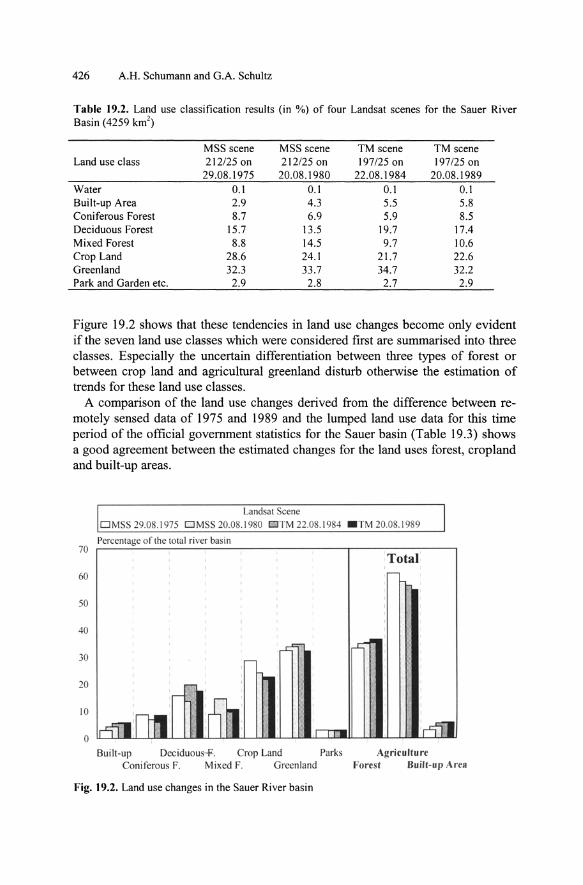
Table 19.2. Land use classification results (in %) of four Landsat scenes for the Sauer River Basin (4259 km2)

MSS scene MSS scene TM scene TM scene Land use class 212125 on 212125 on 197/25 on 197/25 on

29.08.1975 20.08.1980 22.08.1984 20.08.1989 Water 0.1 0.1 0.1 0.1 Built-up Area 2.9 4.3 5.5 5.8 Coniferous Forest 8.7 6.9 5.9 8.5 Deciduous Forest 15.7 13.5 19.7 17.4 Mixed Forest 8.8 14.5 9.7 10.6 Crop Land 28.6 24.1 21.7 22.6 Greenland 32.3 33.7 34.7 32.2 Park and Garden etc. 2.9 2.8 2.7 2.9

Figure 19.2 shows that these tendencies in land use changes become only evident if the seven land use classes which were considered first are summarised into three classes. Especially the uncertain differentiation between three types of forest or between crop land and agricultural greenland disturb otherwise the estimation of trends for these land use classes.

A comparison of the land use changes derived from the difference between re­motely sensed data of 1975 and 1989 and the lumped land use data for this time period of the official government statistics for the Sauer basin (Table 19.3) shows a good agreement between the estimated changes for the land uses forest, cropland and built-up areas.

Landsat Scene 29.08.1975 DM 20.08.1980 DTM 22.08. 1984 . TM 20.08. 1989

Percentage of the total river basin 70

60

50

40

30

20

10

o

Fig. 19.2. Land use changes in the Sauer River basin

Total

19 Detection of Land Cover Change 427

Table 19.3. Land use changes in % for the Sauer basin between 1975 ad 1989 estimated by officia11and use statistics and remote sensing

Land use

forest

cropland

greenland

Land use statistics

+ 3,49 %

-4,15 %

+ 0,42 %

remote sensing

+3,3 %

-6,0%

+0,1 %

The land use maps for the Sauer basin which were derived from the Landsat scenes of 1975 and 1989 are displayed in Colour Plate 19.A. A detailed compari­son of both maps shows that the land use changes are unevenly distributed within the Sauer river basin. Large changes of the built-up areas become evident in the southern part of the river basin where the city of Luxembourg is located. Also the reduction of cropland becomes more obvious in the South-western part of the catchment. For more detailed consideration of the heterogeneity of land use change within the river basin it was sub-divided into eight sub-catchments with drainage areas between 234 and 948 km2 (Fig. 19.3).

For each sub-catchment the differences in land use between 1975 and 1989 were estimated by comparison of the classification results of the two Landsat scenes (Table 19.4). In the catchment of the Alzette river, a tributary of the Sauer river the land use changes by urbanisation were most evident (Colour Plate 19.B).

The estimated increase of the built-up area from 7.2 to 16.3 % is partially due to the different resolution of the different hind use scenes, e.g. the line structures of the highways, which can be seen in the scene of 1989 are hidden by the coarser resolution of the MSS-scene from 1975. The effect of the spatial resolution of the land use classifications is discussed in greater detail below.

Scale problems in land use change detection. For large catchments the high resolution of the Landsat TM data provides an enormous amount of data. There­fore for hydrological modeling a spatial aggregation of the original data becomes necessary. The accuracy of land use classification depends to a certain degree on the spatial resolution (raster or pixel size) of the analysis. To demonstrate this scale effect the Landsat TM scene of 1989 with an original resolution of 30 m was reassembled to 50 m, 250 m, 500 m, 1000 m, 2000 m and 5000 m (Colour Plate 19.C). For aggregation the dominating type of land use within each new raster element was used to classify the total pixel. The effects of an aggregation of land use characteristics is mostly affected by their spatial heterogeneity (Table 19.5). Small land use units disappear, while the portion of the main land use classes is increased.

This effect may be significant for hydrological modelling as it limits the number of available land use classes. If we combine for example the two classes "green­land" and "crop land" to an new class "Agricultural land" the percentage of this main class is less affected by the scale effect than those from the two sub-classes. The portion of the land use class "Built- up area" depends strongly on the spatial

428 A.H. Schumann and G.A. Schultz

6°

25 00

Sub-catchments of the Sauer Basin

1: Nims/A lsdorf

2: A"um'A"umzurlay

3: Our/GelTiind

4: Sauer/Michelau H55 50

50°

H 55 00

49°30'

5: AttertiColmar-Berg

6: Atzette/Ettelbruck

7: Sauer/Boliendorf

8: Sauer/Miindung

5°30'

R25 00

6°

Fig. 19.3. Sub-catchments in the Sauer River basin

6°30'

R 25 50

H 55 50

50°

H 55 00

~Okm

49°30'

6°30'

resolution of land use classification as a coarser resolution reduces the number of pixels which belong to this class significantly. This example shows, that a consid­eration of smaller land use patterns demands a higher resolution of the remote sensing data and of the results of land use characteristics. If a coarser differentia­tion is seen as sufficient with regard to the hydrological model to be used and/or the general aim of the model application an aggregation of the input data seems adequate.

Tab

le 1

9.4.

Diff

eren

ces

in la

nd u

se f

or e

ach

of th

e 8

sub-

catc

hmen

ts o

f the

Sau

er R

iver

bet

wee

n 19

75 a

nd 1

989

resu

lting

fro

m tw

o L

ands

at s

cene

s 19

75 a

nd

1989

Als

dorf

Pr

iimzu

rlay

Gem

iind

Mic

hela

u C

olm

ar-B

erg

Ette

lbru

ck

Bol

lend

orf

Miin

dung

L

and

use

Nim

s Pr

om

Our

Sa

uer

Atte

rt A

lzet

te

Saue

r Sa

uer

(ink

m2)

L7

5*

L89*

L7

5 L8

9 L7

5 L8

9 L7

5 L8

9 L7

5 L8

5 L7

5 L8

9 L7

5 L8

9 L7

5 L8

9 W

ater

0.

0 0.

0 0.

3 0.

3 0.

1 0.

1 2.

4 2.

8 0.

0 0.

0 0.

2 0.

2 0.

7 1.

0 0.

1 0.

4 B

uilt-

up

9.5

15.1

8.

8 17

.1

7.6

10.5

13

.0

27.4

3.

9 12

.9

48.8

11

0.2

8.7

22.4

9.

7 14

.4

Con

ifero

us f

ores

t 23

.0

23.9

61

.5

60.9

11

2.9

1l0.

2 10

6.0

112.

0 12

.3

9.9

23.6

8.

5 34

.6

28.4

5.

6 4.

0 D

ecid

uous

for

est

29.4

32

.8

70.7

86

.8

76.9

84

.7

161.

9 14

6.9

53.8

53

.1

99.4

14

3.1

108.

6 12

8.0

25.6

41

.9

Mix

ed f

ores

t 19

.2

22.2

55

.7

64.3

56

.9

63.8

82

.4,

105.

2 22

.2

36.4

54

.6

56.2

59

.9

73.6

22

.9

23.9

C

rop

land

74

.1

74.2

17

4.0

129.

5 11

9.4

129.

8 22

2.0

206.

9 12

1.1

73.0

22

0.5

130.

5 18

2.9

130.

7 88

.5

72.3

G

reen

land

98

.1

84.2

18

4.8

191.

7 22

0.5

191.

3 32

5.5

307.

5 98

.4

127.

7 20

5.4

211.

6 15

9.0

173.

5 70

.7

68.0

Pa

rk a

nd G

arde

n 8.

0 8.

8 18

.9

24.0

18

.0

21.8

25

.6

30.1

5.

9 4.

5 22

.7

15.0

14

.6

11.4

7.

3 5.

4 Su

m:

261.

2 26

1.2

574.

6 57

4.6

612.

2 61

2.2

938.

9 93

8.9

317.

5 31

7.5

675.

1 67

5.1

569.

1 56

9.1

230.

3 23

0.3

Land

use

(i

n%)

L75

L89

L75

1.89

L7

5 L8

9 L7

5 L8

9 L7

5 L8

9 L7

5 L8

9 L7

5 L8

9 L7

5 L8

9 W

ater

0.

0 0.

0 0.

1 0.

1 0.

0 0.

0 0.

3 0.

3 0.

0 0.

0 0.

0 0.

0 0.

1 0.

2 0.

0 0.

2 B

uilt-

up

3.6

5.8

1.5

3.0

1.2

1.7

1.4

2.9

1.2

4.1

7.2

16.3

1.

5 3.

9 4.

2 6.

2 Fo

rest

27

.4

30.2

32

.7

36.8

40

.3

42.2

37

.3

38.8

27

.8

31.3

26

.3

30.8

35

.7

40.4

23

.5

30.4

A

gric

ultu

re

69.0

64

.0

65.8

60

.1

58.5

56

.1

61.0

58

.0

71.0

64

.6

66.5

52

.9

62.7

55

.5

72.3

31

.4

*L 75

: la

nd u

se 1

975

(Bas

is M

SS).

*L89

: la

nd u

se 1

989

(Bas

is T

M)

-I,Q i a. g So i W f ~

430 A.H. Schumann and G.A. Schultz

Table 19.5. Percental area extension of land use classes for the Sauer River Basin for different aggregation levels of the original 30m x 30m Landsat TM scene of August 1989

Raster width in m

Land use 30 In 50m 200m 500m 1000 m

Built-up Area 5.8 5.8 3.5 3.0 2.7

Forest 36.5 36.4 38.1 40.0 42.3

Greenland 32.2 35.1 37.1 38.5 40.4

Crop Land 22.6 22.6 21.2 18.4 14.5

Agricultural Land 54.8 57.7 58.3 56.9 54.9

Hydrological modelling. After estimation of the land use changes within the Sauer river basin their hydrological effects were described by a hydrological model. This model was also used for scenario analyses of possible future land use changes to describe their hydrological aspects. The model structure based on a sub- division of a watershed into area elements of "Hydrologically Similar Units (HSUs)" in analogy to the Hydrological Response Units of the PRMS-model. As criteria of similarity the following 5 characteristics were selected: -land use - elevation - soil texture classes - slope - exposition. These different characteristics were organised into classes, e.g. the land use was represented by the six classes: water, build-up areas, coniferous forest, deciduous forest, cropland and greenland. The classification which was used for the Sauer river basin is described in Table 19.6. The number of HSUs which was derived by combination of all these classes amounted to 542. For each of these Hydrologically Similar Units the water balance was computed in a daily time step. The model structure is shown schematically in Fig. 19.4.

Table 19.6. Classes of similarity for different physical characteristics within the Sauer River Basin

Similarity At­tributes Elevation

Slope Exposition Soil Land use

number of classes

5

3 3 3 6

Classes

< 300 m, 300-400 m, 400-500 m, 500-600 m, >600m 0-4°,4-12°,2:12° 0-60° and 300°-360°, 120°-240°,240°-300° soil texture: sandy loam, silty loam, clay loam water, built-up areas, coniferous forest, deciduous forest, cropland, greenland

19 Detection of Land Cover Change 431

In order to identify the different HSU's an overlay of the five attribute types was performed within the Geographic Information System in which these data were stored. By application of spatially distributed land use data it became possible to consider the specific hydrological effects of changes dependent on the specific location where these changes occurred. In this way it was e.g. possible to consider the fact that the hydrological effects of urbanisation depend strongly on the soil type which is paved. Obviously lumped modelling and characterisation of land use change would not be appropriate to describe these spatially variable impacts. By consideration of the spatial distribution of land use changes the non-linear impact of such changes on the hydrological processes can be considered, e.g. depends on the reduction of the evapotranspiration as a result of deforestation mostly from the energy and water amounts which are available for this process. In order to specify the impact of changes in land use realistically the specific characteristics: soil, elevation, slope and exposition which are relevant for the energy and water fluxes must be known.

The model was used in three steps. First it was calibrated for the period 1978 to 1983. Then two different land use characteristics, one of 1975 and the other of 1989, were used to compute the water balance of the total period from 1.1.1970 to 31.12.1987. Finally the estimated land use changes of the period from 1975 to 1989 were extrapolated into the future. For extrapolation a time step of 20 years was chosen. As an example in Colour Plate 19.D the land use map for the catch­ment of the river Alzette of 1989 is shown together with a scenario of further de-

groundwater reservoir I base

flow

evapoIranspimtion precipillltion Hydrological

inle .... ception storage

soil

I Similar Unit

1'-TC '1-· s:::=.. ~---' storage -land use, -elevation, -exposition. l, [SIIrftu:e "';"'ff ~ :~~::nent

inteljl~ .. direct ",noff storage r--=----.

" percolation

Fig. 19.4. Structure of the hydrological model for the Sauer River Basin

432 A.H. Schumann and G.A. Schultz

velopment for the year 2009. This catchment is affected strongly by urbanisation as the city of Luxembourg is located in it. In Fig. 19.5 the resulting changes in the seasonal runoff distribution are shown. The runoff in summer (April to September) is increased by a reduced infiltration capacity which leads to an increase of surface runoff in these months with high precipitation intensities. In the winter (October to February) the runoff is slightly reduced. The computed changes in the runoff dis­tribution were not observed in the measured runoff data. The signal of changes in land use between 1975 and 1989 in its effects on the water balance seems to be hidden by errors of discharge and precipitation measurements.

19.4 Summary

Under the aspects of Global Change the concern about land cover changes and their impact ofhydrolgical conditions is growing. Only by remote sensing data it is possible to analyse the changes in land use in nearly real- time and with adequate spatial resolution. Remote sensing offers unique opportunities to get consistent land use characteristics from large areas. Especially for international river basins the problems of different national mapping procedures and different scales and actuality of these maps can be overcome. Land use data derived from remote

60

50

40

30

20

iO

0

6

4

2

o -2

-4

-6

Mean Mon River Ettelbruck

1989 D Scenario 2009

January March May Juli September November RUlloff C hange in Inlll (urll;ln development from 1975 to srenario 2009)

January March May Ju ly September November

Fig. 19.5. Simulated changes of the seasonal runoff distribution as a result of urbanisation in the catchment of the river Alzette

19 Detection of Land Cover Change 433

sensing are an ideal data base for distributed hydrological modelling. Nevertheless some limitations should be considered. The spatial resolution of land use data should be suitable for the scale of the expected land use change. If a coarse spatial resolution is chosen land uses of a relatively small extent may be hidden. If the spatial resolution of classification is too fme the huge amount of data complicates the data management. Another problem of land cover change detection consists in the limited possibility to characterise their hydrological impacts. Usually the hy­drometric networks are not sufficient to estimate the resulting hydrological changes. By utilization of physically based models the possible hydrological ef­fects of land cover changes can be assessed. The precondition of such assessments is a hydrological model which represents the resulting changes in hydrological processes with adequate accuracy. Only distributed hydrological models are able to consider the complexity of hydrological effects which may result from changes of land use. These effects can be strengthened or mitigated by the specific charac­teristics of the locations where these changes occur. Under these aspects a high accuracy of land use classification is needed to represent not only the total amount of land cover changes but also their spatial distribution.

References Abbott, M.B., Bathurst, J.C., Cunge, J.A., O'Connel, P.E., Rasmussen, J. (1986) An introduction

to the European Hydrological System - Systeme Hydrologique "SHE". Journal of Hydrology 87, pp. 45-59

Ah\crona, E. (1995) CORINE Land Cover - A pilot project in Sweden. In: Askne (ed.) "Sensors and Environmental Applications of Remote' Sensing", Proceedings of the 14th EARSel Sym­posium, Goteborg, Sweden, 6-8 June 1994, Balkema, Rotterdam

Allewijn R., Baker H.C. (I 993} Comparison of Landsat TM land use classifications and spatial aggregation as input for an environmental hydrological model. In: Winkler (ed.) "Remote Sensingfor Monitoring the Changing Environment of Europe", Balkema, Rotterdam

Baumgartner,A. (1970) Water- and energy balance of different vegetation covers. IAHS- Pro­ceedings of the Reading Symposium "World Water Balance"

Defries, R. S., Townshend J. R. G. (I 994} NDVI-Derived Land Cover Classifications at a Global Scale. International Journal of Remote Sensing 15, pp. 3567-3586

Dunn, S.M., Mackay, R. (1995) Spatial variation in evapotranspiration and the influence of land use on catchment hydrology. Journal of Hydrology 171, pp. 49-73

Fuller,R., Brown,N. (1996) A CORINE map of Great Britain by automated means. Techniques for automatic generalization of the Land Cover Map of Great Britain. International Journal of Geographical Information Systems 8

Imhoff, M.L. (1994) Mapping Human Impacts on the Global Biosphere. BioScience 44, pp. 598 IPCC (1996) Climate Change 1995, The Science of Climate Change, Cambridge University

Press Klemes, V. (1986): Operational testing of hydrological simulation models. Hydrological Sci­

ences Journal 31, 1 Leavesley G.H., Stannard L.G. (1995) The Precipitation- Runoff Modelling System PRMS. In:

Singh, V.P. (Ed.) Computer Models of Watershed Hydrology, Water Resources Publications Maidment, D.R. (1993) (ed.) Handbook of Hydrology. Mc Graw-Hill Inc. Mehlhorn,H., Rohrle,B. (1990) Die Nitratbelastung der Grundwasservorkommen und MaB­

nahmen zur Reduzierung der Belastung. Wasserwirtschaji 80, H.1O

434 A.H. Schumann and G.A. Schultz

Nandakumar, N., Mein R.G. (1997) Uncertainty in rainfall- runoff model simulations and the implications for predicting the hydrologic effects of land use change. Journal of Hydrology 192, pp. 211-232

Robinson,M., Gannon,B" Schuch,M. (1991) A comparison of the hydrology of moorland under natural conditions, agricultural use and forestry. Hydrological Sciences Journal 36, 6

Schumann, A.H. (1993) Development of conceptual semi-distributed hydrological models and estimation of their parameters with the aid of GIS. Hydr .. Sciences Journal 38, 6

Skole, D., and C. Tucker (1993) Tropical Deforestation and Habitat Fragmentation in the Ama­zon: Satellite Data from 1978 to 1988. Science 260, pp. 1905-1910

root depth [J I '" dorh·.d from

[J . 28'" landu,. ,. " ,. d a..;;sification

(LANDSAT TM) Kl h.lflo'ld .. ,

Colour Plates of Chaps. 16-19 435

• wm~r • urbnn 20<:01

• pa.~turc 45 cm

o agriculture 55 em

• forcs' l 25cm

storaae capacity of the upper soiIla;yer = porosity • roo! depth

-t·

Dc

~ QI1

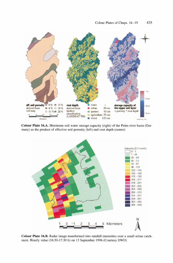
Colour Plate 16.A. Maximum soil water storage capacity (right) of the Priim river basin (Ger­many) as the product of effective soil porosity (left) and root depth (center)

2 3 4 5 Kilo meters -------

Intensity 10.1 mm/hl 00 - 1

1 - 24 _ 25 - 49 _ 50 - 73

74 - 97 98 - 121 122 - 145 146 169

_ 170 - 193

194 - 217 218 - 241 242 - 265 266 - 289 290 - 313 314 -337 338 361 362 - 385 386 - 409

N

A Colour Plate 16.B. Radar image transformed into rainfall intensities over a small urban catch­ment. Hourly value (16:30-17:30 h) on 13 September 1996 (Courtesy DWD)

436 Colour Plates of Chaps. 16-19

1 Urban

./ drainage area

8

11:10 h

11 :20 h

11 :30 h

5 0 5 10 15 Kliometer9

s

11 :15 h

11 :25 h

_. -:. -~.

11 :36 h

r. • ..

o Otbach catchment

Inte .... ~y [mmlh) o 0.1 - 0.3

_ 0.4 - 1.2 _ 1.3 - 2.6

2.7 - 5.0 5.1 . 10.0 10.1 . 16.0 16.1 · 21 .0

_ 21 .1 - 30.0 _ 30.1 - 41 .0

41.1·48.0 _ 48.1 - 67.0 _ 67.1 - 92.0 _ 92.1 - 109.0 _ 109. 1 • 150.0 _ 150.1 • 245.0

Colour Plate 16.C. Sequence of consecutive radar images over an urban catchment area during a storm on July 23, 1996. Time increments: 5 min, pixel size lkm x lkm

Colour Plates of Chaps. 16-19 437

Colour Plate 17.A. Colour composite of Thematic Mapper band 3 (blue) 4 (red) and 5 (green); Torre de Abraham irrigation scheme, Spain, August 8'", 1997. Boundaries of individual fields indi­cated by the overlain map

Colour Plate 17.B. Colour composite of multitemporal images of the Soil Adjusted Vegetation Index (SAVI) calculated with AVHRR ChI and Ch2 reflectance at 1 km spatial resolution, Aral Sea Basin 1992: SAVI (April)= red; SAVI (June)= green; SAVI (August)= blue; area is 1568 km x 1232 km; greenish areas = irrigated lands (courtesy ofN.E. Di Girolamo, NASA, GSFC.\

438 Colour Plates of Chaps. 16-19

o

Colour Plate 17.C. Ratio of actual evaporation to net radiation minus soil heat flux (evaporative fraction) estimated using the algorithm SEBAL (Bastiaanssen, 1995); Torre de Abraham irriga­tion scheme, Spain, July 18'h 1996

Colour Plate IS.A. Cloud development, Tano River basin, Ghana, West Africa. Two successive Meteosat images of the IR spectral channel

_ w

ater

bu

iltu

p ar

eas

coni

fero

us f

ores

t o

deci

duou

s fo

rest

o

mix

ed f

ore

st

crop

land

o

gree

nlan

d o

pare

s, g

arde

n

land

use

197

5 cl

assi

fied

fro

m L

ands

at M

SS

sce

ne

of

29.0

8.19

75

land

use

198

9 cl

assi

fied

fro

m L

ands

at T

M s

cene

o

f 20

.08.

1989

Col

our

Pla

te 1

9.A

. Lan

d us

e m

aps

of

the

Sau

er r

iver

bas

in d

eriv

ed b

y th

e L

ands

at S

cene

s of

197

5 an

d 19

85

(") o g ... :sl ~ en

o ..., (")

::r"

~ :n ......

0\ .!...

'D

-!>­

w

'-0

Cla

ssif

ied

from

Lan

dsat

MSS

Sce

ne o

f 29

.08

.197

5

coni

rcro

u",

forc

... ,

dccidllou~ fnr

c~1

mix

ed f

ore"

cru

pl:I

I),1

grt..

!cnh

md

pare

'. ga

rden

Cla

ssif

ied

from

Lan

dsat

TM

Sce

ne o

f 20

.08.

1989

Col

our

Pla

te 1

9.B

. Lan

d us

e ch

ange

in

the

Alz

ette

Cat

chm

ent,

Lux

embo

urg

, 19

75 v

s 19

89

:l: o (j o 0- '" "1

"1:l S" '" '" g, (j

::l"'

~ on 0'> I -\0

(30

x 30

m2 )

(5

0 x

50 m

2)

(250

x 2

50 m

2)

( I 00

0 x

1000

111

2)

(200

0 x

2000

m2

) (5

000

x 50

00 m

2)

(500

x 5

00 m

2)

• w

aler

bu

iltup

nrc

a,

con

ifcr

uu

!\ for

c~t

deci

duou

s r or

csl

mix

ed f

orc~

l

• cr

opla

nu

D

gree

nlan

d

D

pare

s. g

arde

n

~ __

.l0k

Co

lou

r P

late

19.

C.

Dif

fere

nces

in

land

use

char

acte

rist

ics

as a

res

ult

of

a re

asse

mbl

ing

of

a L

ands

at T

M s

cene

int

o gr

id e

lem

ents

wit

h di

ffer

ent

reso

luti

on (

subc

atch

men

t o

f th

e A

lzet

te r

iver

)

()

o 0'

t:: .... "0

;;;

;:; '" o ..,.,

()

i:l"

~ ~ -0\ J... 'D

.1>0-

.1>0-

• w

ater

•

buil

tup

area

s •

coni

fero

us f

ores

t ...

...

_ de

cidu

ous

fore

st

mix

ed f

ores

t

• cr

opla

nd

D

gree

nla

nd

D

pare

s. g

arde

n

Cla

ssif

ied

from

Lan

dsat

TM

Sce

ne o

f 20

.08.

1989

S

cena

rio

of f

urth

er u

rban

isat

ion

for

the

year

20

09

Col

our

Pla

te 1

9.D

. Sce

nari

o fo

r th

e fu

rthe

r ur

bani

sati

on o

f th

e A

lzet

te c

atch

men

t un

til t

he y

ear

2009

t N

(j o [ ::l ~ '" s, (j ::r

{J

;n

0- I -'C!