reliability-based structural design of aircraft together...
TRANSCRIPT
American Institute of Aeronautics and Astronautics
1
Reliability-Based Structural Design of Aircraft Together
with Future Tests
Erdem Acar1
TOBB University of Economics and Technology, Söğütözü, Ankara 06560, Turkey
Raphael T. Haftka2, Nam-Ho Kim
3
University of Florida, Gainesville, FL 32611, USA
Merve Türinay4
TOBB University of Economics and Technology, Söğütözü, Ankara 06560, Turkey
Chanyoung Park5
University of Florida, Gainesville, FL 32611, USA
Traditional optimization changes variables that are available in the design stage to optimize
objectives, such as aircraft structural reliability. However, there are many post-design
measures, such as tests and structural health monitoring that reduce uncertainty andfurther
improve the reliability. In this paper, a new reliability-based design framework that can
include post-design uncertainty reduction variables is proposed. Among many post-design
variables, this paper focuses on the number of coupon tests and the number of structural
element tests. Uncertainty in the failure stress prediction, variability due to the finite
number of coupon tests, and uncertainties in geometry and service conditions are studied in
detail. The Bayesian technique is used to update the failure stress distribution based on
results of the element tests. Tradeoff plots of the number of tests, weight and probability of
failure in certification and in service are generated, and finally reliability-based design of
future tests together with aircraft structure is performed for minimum lifecycle cost.
Nomenclature
A = load carrying area (width times thickness) of a small part of the overall structure
beef = bound of associated with failure criterion used while predicting failure in the structural element tests
bt = bound of error in the design thickness, et
bw = bound of error in the design width, ew
eef = error associated with failure criterion used while predicting failure in the structural element tests
ef = error in predicting failure of the entire structure in certification or proof testec
ep = error in load calculation
eσ = error in stress calculation
et = error in the design thickness due to construction errors
ew = error in the design width due to construction errors
DOC = direct operating cost
E( ) = expected value (i.e., mean value)
kd = knockdown factor at coupon level due to use of conservative (B-basis) material properties
kf = additional knockdown factor at the structural level (nominal value is taken as 0.95)
nc = number of coupon tests (nominal value is taken as 50)
1 Assistant Professor, Mechanical Engineering, AIAA Member.
2 Distinguished Professor, Mechanical and Aerospace Engineering, AIAA Fellow.
3 Associate Professor, Mechanical and Aerospace Engineering, AIAA Member.
4 Research Assistant, Mechanical Engineering.
5 Research Assistant, Mechanical and Aerospace Engineering.
American Institute of Aeronautics and Astronautics
2
ne = number of element tests (nominal value is taken as 3)
Na = number of aircraft in a fleet (taken as 1,000)
Nmat = number of materials for which coupon testing is done (taken as 80)
Nelem = number of different types of structural elements tested (taken as 100)
p = cost saving by reducing the structural weight by one unit
Pcalc = calculated design load
Pd = true design load based on the FAA specifications (e.g., gust load specification)
Pf = probability of failure
PFCT = probability of failing certification test
σca = allowable stress (B-basis) from coupon testing
σea = allowable stress (B-basis) from element testing
σa = allowable stress (B-basis) of the entire structure
σcf = failure stress from coupon testing
σef = failure stress of the structural element
(σef)test
= element failure stress measured in tests
(σef)calc = calculated (or predicted) element failure stress
(σef)upd
= updated value of the calculated (or predicted) element failure stress
σf = failure stress of the overall structure
σ = stress in a small part of the overall structure
SF = the FAA load safety factor of 1.5
t = thickness of a small part of the overall structure
vt = effect of variability on the built thickness
vw = effect of variability on the built width
w = width of a small part of the overall structure
Subscripts
built-av = average built value that differs from the design value due to errors in construction
built-var = actual built value that differs from the average built value due to variability in construction
calc = calculated (or predicted) value that differs from the design value due to errors in design
design = design value
true = true value (error free value)
I. Introduction
HE safety of aircraft structures can be achieved by designing the structure against uncertainty and by taking
steps to reduce the uncertainty. Safety factors and knockdown factors are examples of measures used to
compensate for uncertainty during the design process. Uncertainty reduction measures (URMs), on the other hand,
may be employed during the design process or later on throughout the operational lifetime. Examples of URMs for
aircraft structural systems include structural testing, quality control, inspection, health monitoring, maintenance, and
improved structural analysis and failure modeling.
In traditional reliability-based optimization, all uncertainties that are available at the design stage are considered
in calculating the reliability of the structure (e.g., Refs. [1-15]). However, the actual aircraft is much safer, because
after design it is customary to engage in vigorous uncertainty reduction activities using various URMs. It would be
therefore beneficial to include the effects of these planned URMs in the design process [16-19]. It may be even
advantageous to design the URMs together with the structure; for example, trading off the cost of more weight
against the cost of additional tests. It is challenging, though, to model the effect of future URMs in the design
process. In this study, we focus on the structural tests as an example of URMs.
There are few papers in the literature that address the effect of tests on structural safety. Jiao and Moan [20]
investigated the effect of proof tests on structural safety using Bayesian updating. They showed that the proof testing
reduces the uncertainty in the strength of a structure, thereby leading to substantial reduction in probability of
failure. Jiao and Eide [21] explored the effects of testing, inspection and repair on the reliability of offshore
structures. Beck and Katafygiotis [22] addressed the problem of updating a probabilistic structural model using
dynamic test data from structure by utilizing Bayesian updating. Similarly, Papadimitriou et al. [23] used Bayesian
updating within a probabilistic structural analysis tool to compute the updated reliability of a structure using test
T
American Institute of Aeronautics and Astronautics
3
data. They found that the reliabilities computed before and after updating were significantly different. In a previous
paper [24], we aimed to extend the work of these earlier authors in simulating all possible outcomes of future tests,
which would allow the designer to design the tests together with the structure.
In [24] we focused on the effects of structural tests on aircraft safety. We investigated in particular the effect of
the number of coupon and structural element tests on the final distribution of the failure stress. We assumed that the
mean value of the failure stress (mean over a large number of aircraft) is obtained from a failure criterion (e.g., Tsai-
Wu theory [25]) using the results of coupon tests. The initial uncertainty in this mean failure stress reflects the
confidence of the analytical model in this prediction as well as possible error in finite number of coupon tests. The
Bayesian technique is then used to update the mean failure stress distribution considering all possible outcomes of
future element tests. In addition, there is the variability of the failure stress from one aircraft to another or from one
structural component to another. We assumed that this variability is the same as the variability in coupon tests,
which holds only for very large number of coupon tests. In the present paper we take into account the error
associated with obtaining material properties from a finite number of coupon tests.
The objective of the present paper is to perform reliability-based design of aircraft structure together with the
future aircraft structural tests. We assume that besides satisfying a constraint on the probability of failure, the
designer needs to satisfy the FAA regulations for deterministic design. In order to reconcile the two requirements,
we take advantage of the fact that companies often apply additional knockdown factors to design allowables beyond
the FAA requirements. We use thus use a company knockdown factor as a design variable that modulates the
tradeoff between cost and safety. We illustrate the generation of response surface plots of the number of tests,
weight and probability of failure in certification and in service. The paper is organized as follows. The next section
provides the motivation for design of aircraft structures together with future tests. Section III discusses the safety
measures taken during aircraft structural design. Section IV presents a simple uncertainty classification that
distinguishes uncertainties that affect an entire fleet (errors) from the uncertainties that vary from one aircraft to
another in the same fleet (variability). Section V discusses modeling of errors and variability throughout the design
and testing of an aircraft, and probability of failure calculation. Finally, the reliability-based optimization results and
the concluding remarks are given in the last two sections of the paper, respectively.
II. Design of Aircraft Structures Together with Future Tests
According to current practices, determination of the number of structural tests is based on past experience.
However, since structural tests are expensive, there is an incentive to reduce the expenditures for tests without
jeopardizing safety. Intuitively, the number of expensive tests such as component tests and element tests can be
reduced and the number of inexpensive tests such as coupon tests can be increased. However, before making such
decisions, the effects of these tests on aircraft safety need to be assessed.
In this paper, the effect of tests on structural safety is assessed by using Monte Carlo simulation (MCS). It is
assumed that the mean value of the failure stress is obtained from a failure criterion using the results of coupon tests.
To reflect our level of confidence in the prediction of the failure criterion, an initial uncertainty in the mean failure
stress is assumed. Then, Bayesian technique is used to update the mean failure stress distribution considering all
possible outcomes of future element tests. In addition, the variability of the failure stress from one airplane to
another or from one structural component to another is modeled in the simulations. The uncertainty in the failure
stress variability due to the finite number of coupon tests is also modeled in the MCS.
After assessing the effects of tests on safety, simultaneous design of aircraft structures and the number of future
tests will be performed for minimum lifecycle cost. The design variables are chosen as the company knockdown
factor and the number of coupon and element tests. Response surface models are constructed to relate the design
variables to structural weight and structural safety. The response surface models are used to compute the lifecycle
cost (the objective function) and the probability of failure (the constraint). These types of models can also be used
by structural designers as well as company managers for tradeoff analyses and decision making.
III. Safety Measures
As noted earlier, the safety of aircraft structures is achieved by designing these structures to operate well in the
presence of uncertainties and taking steps to reduce the uncertainties. The following gives brief description of these
safety measures.
American Institute of Aeronautics and Astronautics
4
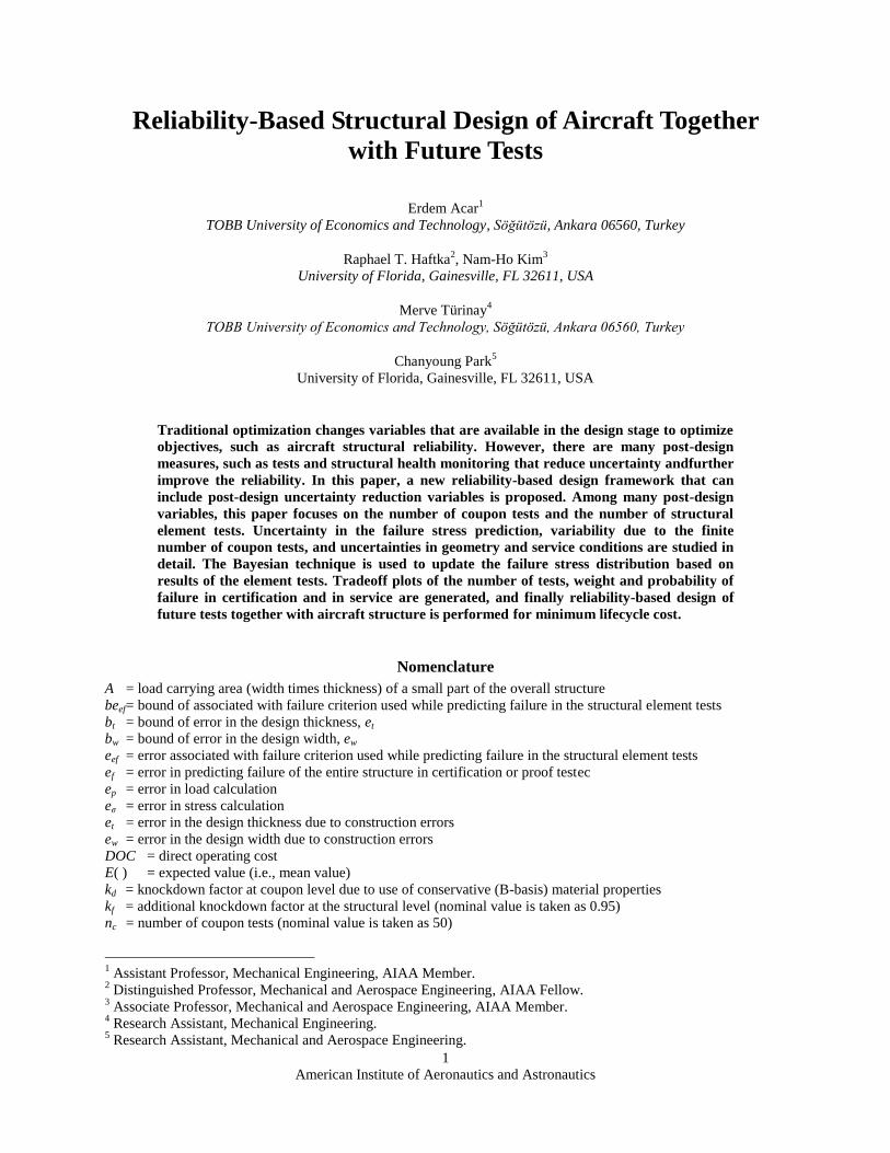
Figure 1. Simplified three-level tests
A. Safety measures for designing structures under uncertainties
Load Safety Factor: In transport aircraft design, FAA regulations mandate the use of a load safety factor of 1.5
(FAR-25.303 [26]). That is, aircraft structures are designed to withstand 1.5 times the limit load without failure.
Conservative Material Properties: In order to account for uncertainty in material properties, FAA regulations
mandate the use of conservative material properties (FAR-25.613 [27]). The conservative material properties are
characterized as A-basis and/or B-basis material property values. Detailed information on these values is provided in
Volume 1, Chapter 8 of the Composite Materials Handbook [28]. In this paper, we use B-basis values. The B-basis
value is determined by calculating the value of a material property exceeded by 90% of the population with 95%
confidence. The basis values are determined by testing a number of coupons selected randomly from a material
batch. In this paper, the nominal number of coupon tests is taken as 50.
Other measures such as redundancy are not discussed in this paper.
B. Safety measures for reducing uncertainties
Improvements in accuracy of structural analysis and failure prediction of aircraft structures reduce errors and
enhance the level of safety. These improvements may be due to better modeling techniques developed by
researchers, more detailed finite element models made possible by faster computers, or more accurate failure
theories. Similarly, the variability in material properties can be reduced through quality control and improved
manufacturing processes. Variability reduction in damage and ageing effects is accomplished through inspections
and structural health monitoring. The reader is referred to the papers by Qu et al. [16] for effects of variability
reduction, Acar et al. [17] for effects of error reduction, and Acar et al. [18] for effects of reduction of both error and
variability.
In this paper, we focus on error reduction through aircraft structural tests, while the other uncertainty reduction
measures are left out for future studies. Structural tests are conducted in a building block procedure (Volume I,
Chapter 2 of Ref. [28]). First, individual coupons are tested to estimate the mean and variability in failure stress. The
mean structural failure is estimated based on failure criteria (such as Tsai-Wu) and this estimate is further improved
using element tests. Then a sub-assembly is tested, followed by a full-scale test of the entire structure. In this paper,
we use the simplified three-level test procedure depicted in Figure 1. The coupon tests, structural element tests and
the final certification test are included.
The first level is the coupon tests, where coupons (i.e., material samples) are tested to estimate failure stress. The
FAA regulation FAR 25-613 requires aircraft companies to perform “enough” tests to establish design values of
material strength properties (A-basis or B-basis value). As the number of coupon tests increases, the errors in the
assessment of the material properties are reduced. However,
since testing is costly, the number of coupon tests is limited to
about 100 to 300 for A-basis calculation and at least 30 for B-
basis value calculation. In this paper, B-basis values are used and
the nominal number of coupon tests is taken as 50.
At the second level of testing, structural elements are tested.
The main target of element tests is to reduce errors related to
failure theories (e.g., Tsai-Wu) used in assessing the failure load
of the structural elements. In this paper, the nominal number of
structural element tests is taken as 3.
At the uppermost level, certification (or proof) testing of the
overall structure is conducted (FAR 25-307 [29]). This final
certification or proof testing is intended to reduce the chance of
failure in flight due to errors in the structural analysis of the
overall structure (e.g., errors in finite element analysis, errors in
failure mode prediction). While failure in flight often has fatal
consequences, certification failure often has serious financial
implications. So we measure the success of the URMs in terms of
American Institute of Aeronautics and Astronautics
5
their effect on probability of failure in flight and in terms of their effect on probability of certification failure.
IV. Structural Uncertainties
A good analysis of different sources of uncertainty in engineering simulations is provided by Oberkampf et al.
[30, 31]. To simplify the analysis, we use a classification that distinguishes between errors (uncertainties that apply
equally to the entire fleet of an aircraft model) and variability (uncertainties that vary for the individual aircraft) as
we used in our earlier studies [32, 33]. The distinction, presented in Table 1, is important because safety measures
usually target either errors or variability. While variabilities are random uncertainties that can be readily modeled
probabilistically, errors are fixed for a given aircraft model (e.g., Boeing 737-400) but they are largely unknown.
Since errors are epistemic, they are often modeled using fuzzy numbers or possibility analysis [34, 35]. We model
errors probabilistically by using uniform distributions because these distributions correspond to minimum
knowledge or maximum entropy.
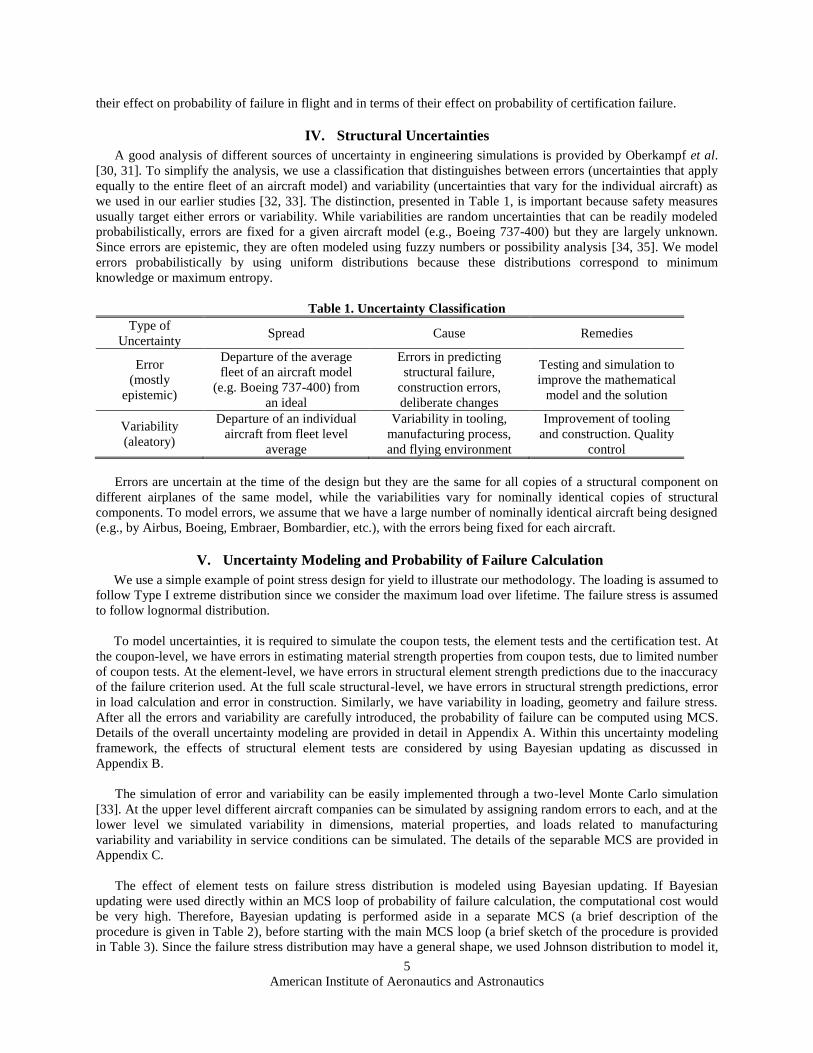
Table 1. Uncertainty Classification
Type of
Uncertainty Spread Cause Remedies
Error
(mostly
epistemic)
Departure of the average
fleet of an aircraft model
(e.g. Boeing 737-400) from
an ideal
Errors in predicting
structural failure,
construction errors,
deliberate changes
Testing and simulation to
improve the mathematical
model and the solution
Variability
(aleatory)
Departure of an individual
aircraft from fleet level
average
Variability in tooling,
manufacturing process,
and flying environment
Improvement of tooling
and construction. Quality
control
Errors are uncertain at the time of the design but they are the same for all copies of a structural component on
different airplanes of the same model, while the variabilities vary for nominally identical copies of structural
components. To model errors, we assume that we have a large number of nominally identical aircraft being designed
(e.g., by Airbus, Boeing, Embraer, Bombardier, etc.), with the errors being fixed for each aircraft.
V. Uncertainty Modeling and Probability of Failure Calculation
We use a simple example of point stress design for yield to illustrate our methodology. The loading is assumed to
follow Type I extreme distribution since we consider the maximum load over lifetime. The failure stress is assumed
to follow lognormal distribution.
To model uncertainties, it is required to simulate the coupon tests, the element tests and the certification test. At
the coupon-level, we have errors in estimating material strength properties from coupon tests, due to limited number
of coupon tests. At the element-level, we have errors in structural element strength predictions due to the inaccuracy
of the failure criterion used. At the full scale structural-level, we have errors in structural strength predictions, error
in load calculation and error in construction. Similarly, we have variability in loading, geometry and failure stress.
After all the errors and variability are carefully introduced, the probability of failure can be computed using MCS.
Details of the overall uncertainty modeling are provided in detail in Appendix A. Within this uncertainty modeling
framework, the effects of structural element tests are considered by using Bayesian updating as discussed in
Appendix B.
The simulation of error and variability can be easily implemented through a two-level Monte Carlo simulation
[33]. At the upper level different aircraft companies can be simulated by assigning random errors to each, and at the
lower level we simulated variability in dimensions, material properties, and loads related to manufacturing
variability and variability in service conditions can be simulated. The details of the separable MCS are provided in
Appendix C.
The effect of element tests on failure stress distribution is modeled using Bayesian updating. If Bayesian
updating were used directly within an MCS loop of probability of failure calculation, the computational cost would
be very high. Therefore, Bayesian updating is performed aside in a separate MCS (a brief description of the
procedure is given in Table 2), before starting with the main MCS loop (a brief sketch of the procedure is provided
in Table 3). Since the failure stress distribution may have a general shape, we used Johnson distribution to model it,
American Institute of Aeronautics and Astronautics
6
which can be represented using four quantiles. The procedure followed for Bayesian updating can be described
briefly as follows. First, the four quantiles of the mean failure stress are modeled as normal distributions. Then,
these quantiles are used to fit a Johnson distribution to the mean failure stress. That is, the mean failure stress is
represented as a Johnson distribution, whose parameters are themselves distributions that depend on the number of
element tests as well as the error in failure stress prediction of the elements, eef. Finally, Bayesian updating is used to
update the mean failure stress distribution as in our earlier work [36].
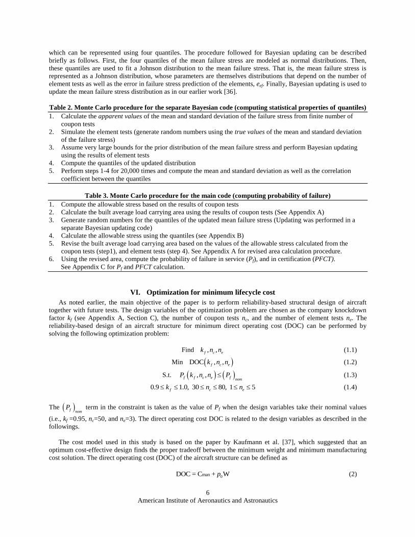
Table 2. Monte Carlo procedure for the separate Bayesian code (computing statistical properties of quantiles)
1. Calculate the apparent values of the mean and standard deviation of the failure stress from finite number of
coupon tests
2. Simulate the element tests (generate random numbers using the true values of the mean and standard deviation
of the failure stress)
3. Assume very large bounds for the prior distribution of the mean failure stress and perform Bayesian updating
using the results of element tests
4. Compute the quantiles of the updated distribution
5. Perform steps 1-4 for 20,000 times and compute the mean and standard deviation as well as the correlation
coefficient between the quantiles
Table 3. Monte Carlo procedure for the main code (computing probability of failure)
1. Compute the allowable stress based on the results of coupon tests
2. Calculate the built average load carrying area using the results of coupon tests (See Appendix A)
3. Generate random numbers for the quantiles of the updated mean failure stress (Updating was performed in a
separate Bayesian updating code)
4. Calculate the allowable stress using the quantiles (see Appendix B)
5. Revise the built average load carrying area based on the values of the allowable stress calculated from the
coupon tests (step1), and element tests (step 4). See Appendix A for revised area calculation procedure.
6. Using the revised area, compute the probability of failure in service (Pf), and in certification (PFCT).
See Appendix C for Pf and PFCT calculation.
VI. Optimization for minimum lifecycle cost
As noted earlier, the main objective of the paper is to perform reliability-based structural design of aircraft
together with future tests. The design variables of the optimization problem are chosen as the company knockdown
factor kf (see Appendix A, Section C), the number of coupon tests nc, and the number of element tests ne. The
reliability-based design of an aircraft structure for minimum direct operating cost (DOC) can be performed by
solving the following optimization problem:
Find , ,f c ek n n (1.1)
Min DOC , ,f c ek n n (1.2)
S.t. , ,f f c e f nomP k n n P (1.3)
0.9 1.0, 30 80, 1 5f c ek n n (1.4)
The f nomP term in the constraint is taken as the value of Pf when the design variables take their nominal values
(i.e., kf =0.95, nc=50, and ne=3). The direct operating cost DOC is related to the design variables as described in the
followings.
The cost model used in this study is based on the paper by Kaufmann et al. [37], which suggested that an
optimum cost-effective design finds the proper tradeoff between the minimum weight and minimum manufacturing
cost solution. The direct operating cost (DOC) of the aircraft structure can be defined as
0manDOC = C + Wp (2)
American Institute of Aeronautics and Astronautics
7
where Cman is the manufacturing cost, p0 is the cost penalty due to excessive structural weight, W. In our study, we
modify this cost formulation to take into account the cost of the uncertainty reduction measures (Curm) including
tests, quality control, health monitoring, etc. In addition, we dump the manufacturing cost into the cost of excess
weight. That is, the DOC is reformulated as
urmDOC = W + Cp (3)
Here, p is the total cost saving attained by reducing the structural weight by one pound. In this study, amongst
uncertainty reduction measures (URMs) noted earlier, we focus on tests. Hence, Curm is divided into two elements as
urm test urm-otherC = C + C (4)
where Ctest is the cost of tests, and Curm-other is the total cost of URMs other than tests. In this study, we focus mainly
on two types of tests: the coupon tests and the element tests. Thus, Ctest can be re-written as
test coupon elem test-otherC = C + C + C (5)
where Ccoupon is the cost of coupon tests, Celem is the cost of element tests, and Ctest-other is the cost of other tests such
as component tests, assembly tests, certification test, etc.
Equations (2-4) can be combined to yield
coupon elem otherDOC = W + C + C + Cp (6)
where
other urm-other test-other laborC = C + C + C (7)
The direct operation cost can be re-written so as to show its dependence on the knockdown factor kf, the number of
coupon tests nc, and the number of element tests ne as
elem otherDOC , , = W , , + C + C + Cf c e f c e coupon c ek n n p k n n n n (8)Here, W is the structural weight, p is
the weight penalty, Cc is the cost of coupon tests, Ce is the cost of element tests, and Cother refers to the costs that are
not affected by the choice of design variables. Since DOC is used within an optimization framework, Cother term can
be dropped. Details of each term in the cost equation are provided below.
Weight penalty p
Curran et al. [38] proposed that the economical value of weight saving is 300 $/kg. Similarly, Kim et al. [39]
referred to a recent report by the US National Materials Advisory Board [40] that estimated that a 1 lb weight
reduction amounts to a total saving of $200 for a civil transport aircraft. In our study, we vary the weight penalty
between $200/lb and $1000/lb and see its effect on the optimum values of the design variables.
The structural weight
We take the structural weight of a typical civil transport aircraft as 50,000 lbs. Since the test costs can be attributed
to fleet of aircraft rather than a single one, total structural weight of the fleet is considered. Therefore, the weight
term in Eq. (8) can be written as
, ,
W , , 50,000cert f c e
f c e a
nom
A k n nk n n N
A (9)
Here Acert is the certified load carrying area, and Anom is the value of Acert when the design variables take their
nominal values. We assume that a typical airliner has a production line of 1,000 aircraft before it is discontinued or
substantially redesigned, so Na=1,000.
American Institute of Aeronautics and Astronautics
8
Test costs
The costs for the coupon tests and element tests are based on personal communications with structural engineers in
Turkish Aerospace Industries, Boeing, and NASA. They are taken as $300 for each coupon in a coupon test, and
$150,000 for each element tests. Accordingly the respective costs are given as
Ccoupon (nc) = 300×Nmat×nc (in $) (10)
Celem (ne) = 150,000×Nelem×ne (in $) (11)
where the Nmat is the number of different materials tested for a single aircraft model, and Nelem is the number
different types of structural elements tested. In this study, these values are taken as Nmat=80, and Nelem=100,
respectively.
If the design variables take their nominal values, and p=$200/lb, the DOC is
6 DOC = 200 1,000 50,000 + 300 80 50 + 150,000 100 3= 10,000+1.2+45 10 dollars (12)
According to Eq. (12), even for the lowest weigh penalty, the contribution of weight to the cost dominates the cost
of tests. So if we can reduce the weight by more than 0.15% by performing an additional element test, then we
should choose to do that. This reflects the large number of airplanes (assumed to be 1,000 here) that benefit from the
results of the test. We will investigate these tradeoffs in detail in the Results section.
VII. Results
In this section, first the effects of the number of coupon tests and the number of element tests on the weight and
probability of failure will be investigated. Then, the reliability-based design of aircraft will be performed for
minimum direct operating cost.
A. Response surface generation for weight and reliability index in terms of the design variables
Response surface models (quadratic polynomial with all terms included) are constructed to relate the number of
structural tests, and company knock down factors to structural weight, and structural safety for use in the
optimization. The input variables of the response surface models and their bounds are provided in Table 4. Latin
hypercube design of experiments is used to generate thirty training points within the bounds given in Table 4. The
built average load carrying area (surrogate for the structural weight) and the probability of failure are computed
using Monte Carlo simulations. The accuracies of the constructed response surface models are evaluated by using
leave-one-out cross-validation errors. Response surface models are constructed 30 times, each time leaving out one
of the training points. The difference between the exact response at the omitted point and that predicted by each
variant response surface model defines the cross-validation error. Table 5 provides the root mean square error
(RMSE), the maximum absolute error (MAE), the maximum absolute error (MAXE) as well as the mean of the
response. Comparison of the error metrics to the mean of response reveals that the constructed response surfaces are
quite accurate.
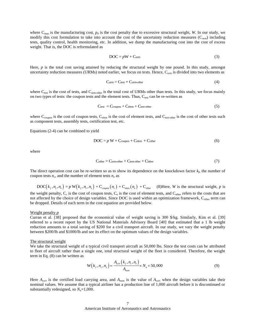
Table 4. Input variables of the response surface models and their bounds
Variable kf nc ne
Lower bound 0.90 30 1
Upper bound 1.00 80 5
Table 5. Evaluating accuracies of response surface models using leave-one-out cross validation errors
Response Mean of response RMSE(a)
MAE(b)
MAXE(c)
Acert 1.24 0.0015 0.0011 0.0041
Rel. Index, β 5.24 0.009 0.008 0.018 (a)
RMSE: root mean square error; (b)
MAE: mean absolute error; (c)
MAXE: maximum absolute error
American Institute of Aeronautics and Astronautics
9
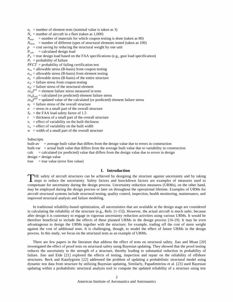
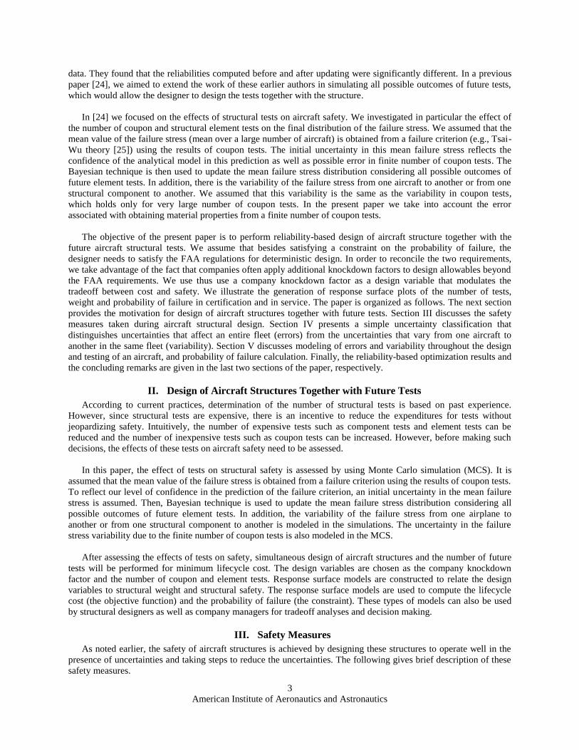
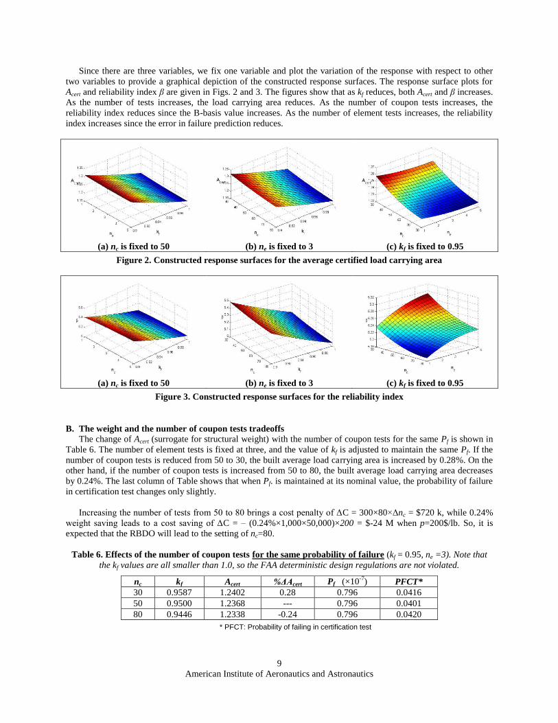
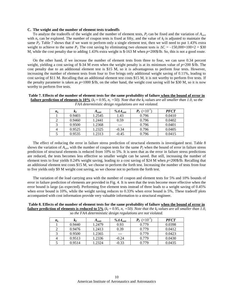
Since there are three variables, we fix one variable and plot the variation of the response with respect to other
two variables to provide a graphical depiction of the constructed response surfaces. The response surface plots for
Acert and reliability index β are given in Figs. 2 and 3. The figures show that as kf reduces, both Acert and β increases.
As the number of tests increases, the load carrying area reduces. As the number of coupon tests increases, the
reliability index reduces since the B-basis value increases. As the number of element tests increases, the reliability
index increases since the error in failure prediction reduces.
(a) nc is fixed to 50 (b) ne is fixed to 3 (c) kf is fixed to 0.95
Figure 2. Constructed response surfaces for the average certified load carrying area
(a) nc is fixed to 50 (b) ne is fixed to 3 (c) kf is fixed to 0.95
Figure 3. Constructed response surfaces for the reliability index
B. The weight and the number of coupon tests tradeoffs
The change of Acert (surrogate for structural weight) with the number of coupon tests for the same Pf is shown in
Table 6. The number of element tests is fixed at three, and the value of kf is adjusted to maintain the same Pf. If the
number of coupon tests is reduced from 50 to 30, the built average load carrying area is increased by 0.28%. On the
other hand, if the number of coupon tests is increased from 50 to 80, the built average load carrying area decreases
by 0.24%. The last column of Table shows that when Pf. is maintained at its nominal value, the probability of failure
in certification test changes only slightly.
Increasing the number of tests from 50 to 80 brings a cost penalty of ΔC = 300×80×Δnc = $720 k, while 0.24%
weight saving leads to a cost saving of ΔC = – (0.24%×1,000×50,000)×200 = $-24 M when p=200$/lb. So, it is
expected that the RBDO will lead to the setting of nc=80.
Table 6. Effects of the number of coupon tests for the same probability of failure (kf = 0.95, ne =3). Note that
the kf values are all smaller than 1.0, so the FAA deterministic design regulations are not violated.
nc kf Acert %ΔAcert Pf (×10-7
) PFCT*
30 0.9587 1.2402 0.28 0.796 0.0416
50 0.9500 1.2368 --- 0.796 0.0401
80 0.9446 1.2338 -0.24 0.796 0.0420
* PFCT: Probability of failing in certification test
American Institute of Aeronautics and Astronautics
10
C. The weight and the number of element tests tradeoffs
To analyze the tradeoffs of the weight and the number of element tests, Pf can be fixed and the variation of Acert
with ne can be explored. The number of coupon tests is fixed at fifty, and the value of kf is adjusted to maintain the
same Pf. Table 7 shows that if we want to perform only a single element test, then we will need to put 1.43% extra
weight to achieve to the same Pf. The cost saving by eliminating two element tests is ΔC = –150,000×100×2 = $30
M, while the cost penalty due to adding 1.43% extra weight is $-163 M when p=200$/lb. So, this is not a good route.
On the other hand, if we increase the number of element tests from three to four, we can save 0.34 percent
weight, yielding a cost saving of $-34 M even when the weight penalty is at its minimum value of p=200 $/lb. The
cost penalty due to an additional element test is $15 M, so it is advantageous to perform four tests. However,
increasing the number of element tests from four to five brings only additional weight saving of 0.11%, leading to
cost saving of $11 M. Recalling that an additional element test costs $15 M, it is not worthy to perform five tests. If
the penalty parameter is taken as p=1000 $/lb, on the other hand, the weight cost saving will be $30 M, so it is now
worthy to perform five tests.
Table 7. Effects of the number of element tests for the same probability of failure when the bound of error in
failure prediction of elements is 10% (kf = 0.95, nc =50). Note that the kf values are all smaller than 1.0, so the
FAA deterministic design regulations are not violated.
ne kf Acert %ΔAcert Pf (×10-7
) PFCT
1 0.9403 1.2545 1.43 0.796 0.0410
2 0.9460 1.2441 0.59 0.796 0.0402
3 0.9500 1.2368 --- 0.796 0.0401
4 0.9525 1.2325 -0.34 0.796 0.0405
5 0.9535 1.2313 -0.45 0.796 0.0415
The effect of reducing the error in failure stress prediction of structural elements is investigated next. Table 8
shows the variation of Acert with the number of coupon tests for the same Pf when the bound of error in failure stress
prediction of structural elements is reduced from 10% to 5%. It is seen that as the error in failure stress predictions
are reduced, the tests becomes less effective so smaller weight can be saved. But still, increasing the number of
element tests to four yields 0.24% weight saving, leading to a cost saving of $24 M when p=200$/lb. Recalling that
an additional element test costs $15 M, we choose to perform the forth test. Increasing the number of tests from four
to five yields only $9 M weight cost saving, so we choose not to perform the forth test.
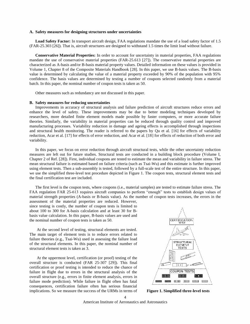
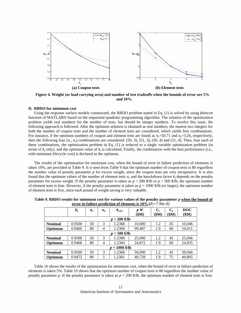
The variation of the load carrying area with the number of coupon and element tests for 5% and 10% bounds of
error in failure prediction of elements are provided in Fig. 4. It is seen that the tests become more effective when the
error bound is large (as expected). Performing five element tests instead of three leads to a weight saving of 0.45%
when error bound is 10%, while the weight saving reduces to 0.33% when error bound is 5%, These tradeoff plots
accompanied with cost information provide very valuable information to a structural engineer.
Table 8. Effects of the number of element tests for the same probability of failure when the bound of error in
failure prediction of elements is reduced to 5% (kf = 0.95, nc =50). Note that the kf values are all smaller than 1.0,
so the FAA deterministic design regulations are not violated.
ne kf Acert %ΔAcert Pf (×10-7
) PFCT
1 0.9440 1.2479 0.93 0.779 0.0398
2 0.9476 1.2413 0.39 0.779 0.0412
3 0.9500 1.2365 --- 0.779 0.0423
4 0.9513 1.2336 -0.24 0.779 0.0430
5 0.9514 1.2324 -0.33 0.779 0.0435
American Institute of Aeronautics and Astronautics
11
(a) Coupon tests (b) Element tests
Figure 4. Weight (or load carrying area) and number of test tradeoffs when the bounds of error are 5%
and 10%.
D. RBDO for minimum cost
Using the response surface models constructed, the RBDO problem stated in Eq. (1) is solved by using fmincon
function of MATLAB® based on the sequential quadratic programming algorithm. The solution of the optimization
problem yields real numbers for the number of tests, but should be integer numbers. To resolve this issue, the
following approach is followed. After the optimum solution is obtained as real numbers, the nearest two integers for
both the number of coupon tests and the number of element tests are considered, which yields four combinations.
For instance, if the optimum numbers of coupon and element tests are found as nc=50.71 and ne=3.26, respectively,
then the following four (nc, ne) combinations are considered: (50, 3), (51, 3), (50, 4) and (51, 4). Then, four each of
these combinations, the optimization problem in Eq. (1) is reduced to a single variable optimization problem (in
terms of kf only), and the optimum value of kf is calculated. Finally, the combination with the best performance (i.e.,
with minimum lifecycle cost) is declared as the optimum.
The results of the optimization for minimum cost, when the bound of error in failure prediction of elements is
taken 10%, are provided in Table 9. It is seen from Table 9 that the optimum number of coupon tests is 80 regardless
the number value of penalty parameter p for excess weight, since the coupon tests are very inexpensive. It is also
found that the optimum values of the number of element tests ne and the knockdown factor kf depends on the penalty
parameter for excess weight. If the penalty parameter is taken as p = 200 $/lb or p = 500 $/lb, the optimum number
of element tests is four. However, if the penalty parameter is taken as p = 1000 $/lb (or larger), the optimum number
of element tests is five, since each pound of weight saving is very valuable.
Table 9. RBDO results for minimum cost for various values of the penalty parameter p when the bound of
error in failure prediction of elements is 10%.(Pf=7.96e-8)
kf nc ne Acert p W
($M)
Cc
($M)
Ce
($M)
DOC
($M)
p = 200 $/lb
Nominal 0.9500 50 3 1.2368 10,000 1.2 45 10,046
Optimum 0.9466 80 4 1.2304 99,487 1.9 60 10,011
p = 500 $/lb
Nominal 0.9500 50 3 1.2368 25,000 1.2 45 25,046
Optimum 0.9466 80 4 1.2304 24,872 1.9 60 24,935
p = 1000 $/lb
Nominal 0.9500 50 3 1.2368 50,000 1.2 45 50,046
Optimum 0.9472 80 5 1.2301 49,728 1.9 75 49,805
Table 10 shows the results of the optimization for minimum cost, when the bound of error in failure prediction of
elements is taken 5%. Table 10 shows that the optimum number of coupon tests is 80 regardless the number value of
penalty parameter p. If the penalty parameter is taken as p = 200 $/lb, the optimum number of element tests is four.
American Institute of Aeronautics and Astronautics
12
However, if the penalty parameter is increased to p = 500 $/lb, then the weight saving becomes more important, so
the optimum number of element tests is increased to five.
Table 10. RBDO results for minimum cost for various values of the penalty parameter p when the bound
of error in failure prediction of elements is 5%.(Pf=7.79e-8)
kf nc ne Acert p W
($M)
Cc
($M)
Ce
($M)
DOC
($M)
p = 200 $/lb
Nominal 0.9500 50 3 1.2346 10,000 1.2 45 10,046
Optimum 0.9451 80 4 1.2312 9,957 1.9 60 10,019
p = 500 $/lb
Nominal 0.9500 50 3 1.2346 25,000 1.2 45 25,046
Optimum 0.9460 80 5 1.2294 24,856 1.9 75 24,933
p = 1000 $/lb
Nominal 0.9500 50 3 1.2346 50,000 1.2 45 50,046
Optimum 0.9460 80 5 1.2294 49,713 1.9 75 49,790
VIII. Concluding remarks
Most probabilistic structural design studies assume that the uncertainties are given and resources are used to
compensate for them by making the structure strong enough. Instead, the resources can be allocated for uncertainty
reduction measures, URMs, for reducing uncertainties, which would in turn increase the safety. Similarly, the
increased safety can be traded off for reducing direct operating cost. It would be therefore beneficial to include the
effects of these planned URMs in the design process under uncertainty. This paper proposed probabilistic design of
aircraft structures together with future structural tests using probabilistic methods.
The effects of structural tests on safety of aircraft structures were investigated and, it was found when the bound
of error for failure prediction of structural elements was 10% that
o if the number of coupon tests was increased from 50 to 80 maintaining the same probability of failure, the
structural weight could be reduced by 0.24%.
o if the number of element tests was increased from three to four (or five) maintaining the same probability of
failure, the structural weight can be reduced by 0.34% (or 0.45%).
o if the bounds of error in failure stress prediction of structural elements are reduced, then the tests becomes
less effective and the weight saving reduces.
Reliability-based optimization of aircraft structures was performed and it was found that the optimization results
depend heavily on the penalty for excess weight (p) and the bound of error for failure prediction of structural
elements. It was also found that the optimum number of coupon tests was 80 (maximum considered), regardless the
penalty parameter p and the bound of error, since the coupon tests were very inexpensive. Through solving the
RBDO problem, the followings were observed.
o if the bound of error for failure prediction of structural elements was 10%, the optimum number of element
tests was four when the penalty parameter was p = 500 $/lb (or smaller), and the optimum number of element
tests was five when the penalty parameter is p = 1000 $/lb (or larger).
o if the bound of error for failure prediction of structural elements was 5%, the optimum number of element
tests was four when the penalty parameter was p = 200 $/lb (or smaller), and the optimum number of element
tests was five when the penalty parameter is p = 500 $/lb (or larger).
The results found for various bounds of error for failure prediction of structural elements basically indicated that
if the aircraft companies support research activities that can improve the failure prediction theories, they can reduce
the number of structural tests for the same safety and same lifetime cost.
American Institute of Aeronautics and Astronautics
13
Acknowledgments
This research is partially supported by TÜBİTAK, under award 109M537, and by the NASA center and the U.S. Air
Force, U.S. Air Force Research Laboratory, under award FA9550-07-1-0018 (Victor Giurgiutiu, Program Manager)
and National Science Foundation (CMMI-0927790). The authors gratefully acknowledge these supports.
References
1. Lincoln, J.W., “Method for Computation of Structural Failure Probability for an Aircraft,” ASD-TR-80-5035, Wright–
Patterson AFB, OH, July 1980.
2. Lincoln, J.W., “Risk Assessment of an Aging Aircraft,” Journal of Aircraft, Vol. 22, No. 8, August 1985, pp. 687-691.
3. Shiao, M.C., Nagpal, V.K., and Chamis, C.C., “Probabilistic Structural Analysis of Aerospace Components Using NESSUS,”
AIAA 88-2373, 1988.
4. Wirsching, P.H., “Literature Review on Mechanical Reliability and Probabilistic Design,” Probabilistic Structural Analysis
Methods for Select Space Propulsion System Components (PSAM), NASA CR 189159, Vol. III, 1992.
5. Lykins, C., Thomson, D., and Pomfret, C., “The Air Force‟s Application of Probabilistics to Gas Turbine Engines,” AIAA-
94-1440-CP, 1994.
6. Ebberle, D.H., Newlin, L.E., Sutharshana, S., and Moore, N.R., “Alternative Computational Approaches for Probabilistic
Fatigue Analysis,” AIAA-95-1359, 1995.
7. Ushakov, A., Kuznetsov, A.A., Stewart, A., and Mishulin, I.B., “Probabilistic Design of Damage Tolerant Composite
Aircraft Structures,” Final Report under Annex 1 to Memorandum of Cooperation AIA/CA-71 between the FAA and Central
Aero-Hydrodynamic Institute (TsAGI), 1996.
8. Mavris, D.N., Macsotai, N. I., and Roth, B., “A probabilistic design methodology for commercial aircraft engine cycle
selection,” Paper SAE-985510, Society of Automotive Engineers, 1998.
9. Long, M.W., and Narciso, J.D., “Probabilistic Design Methodology for Composite Aircraft Structures.” DOD/FAA/AR-99/2,
Final Rept., June 1999.
10. Ushakov, A., Stewart, A., Mishulin, I., and Pankov, A., “Probabilistic Design of Damage Tolerant Composite Aircraft
Structures.” DOD/FAA/AR-01/55, Final Rept., January 2002.
11. Rusk, D. T., Lin, K. Y., Swartz, D. D., and Ridgeway, G. K., “Bayesian Updating of Damage Size Probabilities for Aircraft
Structural Life-cycle Management,” AIAA Journal of Aircraft, Vol. 39, No. 4, July 2002, pp. 689-696.
12. Allen, M., and Maute, K., “Reliability-based design optimization of aeroelastic structures,” Structural and Multidisciplinary
Optimization, Vol. 27, 2004, pp. 228–242.
13. Huang, C.K., and Lin, K.Y., “A Method for Reliability Assessment of Aircraft Structures Subject to Accidental Damage,”
AIAA-2005-1830, 2005.
14. Nam, T., Soban, D.S., and Marv‟s, D.N., “A Non-Deterministic Aircraft Sizing Method under Probabilistic Design
Constraints,” AIAA 2006-2062, 2006.
15. Lin, K.Y., and Styuart, A.V., “Probabilistic Approach to Damage Tolerance Design of Aircraft Composite Structures,”
Journal of Aircraft, Vol. 44, No. 4, July-August 2007.
16. Qu, X., Haftka, R.T., Venkataraman, S., and Johnson, T.F., “Deterministic and Reliability-Based Optimization of Composite
Laminates for Cryogenic Environments,” AIAA Journal, Vol. 41, No. 10, 2003, pp. 2029-2036.
17. Acar, E., Haftka, R.T., Sankar, B.V. and Qui, X., "Increasing Allowable Flight Loads by Improved Structural Modeling,"
AIAA Journal, Vol. 44, No. 2, 2006, pp. 376-381.
18. Acar, E., Haftka, R.T. and Johnson, T.F., "Tradeoff of Uncertainty Reduction Mechanisms for Reducing Structural Weight,"
Journal of Mechanical Design, Vol. 129, No. 3, 2007, pp. 266-274.
19. Li M, Williams N, Azarm S (2009) Interval uncertainty reduction and sensitivity analysis with multi-objective design
optimization. J Mech Des 131(3), pp.1–11.
20. Jiao, G., and Moan, T., "Methods of reliability model updating through additional events," Structural Safety, Vol. 9, No. 2,
1990, pp. 139-153.
21. Jiao, G., and Eide, O.I., "Effects of Testing, Inspection and Repair on the Reliability of Offshore Structures," Proceedings of
the Seventh Specialty Conference, Worcester, Massachusetts, August 7-9, 1996, pp. 154-157.
22. Beck, J.L., and Katafygiotis, L.S., "Updating models and their uncertainties: Bayesian Statistical Framework," Journal of
Engineering Mechanics, Vol. 124, No. 4, 1998, pp. 455-461.
23. Papadimitriou, C., Beck, J.L., and Katafygiotis, L.S., "Updating Robust Reliability Using Structural Test Data," Probabilistic
Engineering Mechanics, Vol. 16, No. 2, 2001, pp. 103-113.
24. Acar, E., Haftka, R.T., Kim, N.H., and Buchi, D., "Effects of Structural Tests on Aircraft Safety," 50th
AIAA/ASME/ASCE/AHS/ASC Structures, Structural Dynamics, and Materials Conference, Palm Springs, CA, May 2009.
25. Zhu, H., Sankar, B.V., and Marrey, R.V., “Evaluation of Failure Criteria for Fiber Composites Using Finite Element
Micromechanics,” Journal of Composite Materials, Vol. 32, No. 8, 1998, pp. 766–782.
26. Federal Aviation Regulations, Part 25, Airworthiness Standards: Transport Category Airplanes, Sec. 25.303, Factor of Safety.
27. Federal Aviation Regulations, Part 25, Airworthiness Standards: Transport Category Airplanes, Sec. 25.613, Material
Strength Properties and Material Design Values.
28. Composite Materials Handbook MIL-HDBK-17, “Guidelines for Property Testing of Composites,” ASTM Publications,
2002.
American Institute of Aeronautics and Astronautics
14
29. Federal Aviation Regulations, Part 25, Airworthiness Standards: Transport Category Airplanes, Sec. 25.307, Proof of
Structure.
30. Oberkampf, W.L., Deland, S.M., Rutherford, B.M., Diegert, K.V., and Alvin, K.F., “Estimation of Total Uncertainty in
Modeling and Simulation,” Sandia Report, SAND2000-0824, 2000, Albuquerque, NM.
31. Oberkampf, W.L., Deland, S.M., Rutherford, B.M., Diegert, K.V., and Alvin, K.F., “Error and Uncertainty in Modeling and
Simulation,” Reliability Engineering and System Safety, Vol. 75, 2002, pp. 333-357.
32. Acar, E., Kale, A., Haftka, R.T. and Stroud, W.J., "Structural Safety Measures for Airplanes," Journal of Aircraft, Vol. 43,
No. 1, 2006, pp. 30-38.
33. Acar, E., Kale, A., and Haftka, R.T., "Comparing Effectiveness of Measures that Improve Aircraft Structural Safety," Journal
of Aerospace Engineering, Vol. 20, No. 3, 2007, pp. 186-199.
34. Antonsson, E. K., and Otto, K. N., 1995, “Imprecision in Engineering Design,” ASME J. Mech. Des. 117 pp. 25–32.
35. Nikolaidis, E., Chen, S., Cudney, H., Haftka, R. T., and Rosca, R., 2004, “Comparison of Probability and Possibility for
Design Against Catastrophic Failure Under Uncertainty,” ASME J. Mech. Des. 126, pp. 386–394.
36. An, J., Acar, E., Haftka, R.T., Kim, N.H., Ifju, P.G., and Johnson, T.F., "Being Conservative with a Limited Number of Test
Results," Journal of Aircraft, Vol. 45, No. 6, 2008, pp. 1969-1975.
37. Kaufmann, M., Zenkert, D., and Wennhage, P., “Integrated cost/weight optimization of aircraft structures,” Structural and
Multidisciplinary Optimization, DOI 10.1007/s00158-009-0413-1, 2009.
38. Curran, R., Rothwell, A., and Castagne, S., “Numerical Method for Cost-Weight Optimization of Stringer–Skin Panels,”
Journal of Aircraft, Vol. 43, No. 1, 2006, pp. 264-274.
39. Kim, H.A., Kennedy, D., and Gürdal, Z., “Special issue on optimization of aerospace structures,” Structural and
Multidisciplinary Optimization, Vol. 36, No. 1, 2008, pp. 1-2.
40. Anon., “Materials Research to Meet 21st Century Defense Needs,” Committee on Materials Research for Defense After
Next, National Research Council, ISBN: 0-309-50572-0, 2003. Available from http://www.nap.edu/catalog/10631.html
41. Noh, Y.,•Choi, K.K., and Du, L., “Reliability-based design optimization of problems with correlated input variables using a
Gaussian Copula,” Structural and Multidisciplinary Optimization, Vol. 38, 2009, pp.1-16.
42. Smarslok, B., Haftka, R.T., and Kim, N-H, “Comparison and Efficiency Analysis of Crude and Separable Monte Carlo
Simulation Methods,” 47th AIAA/ASME/ASCE/AHS/ASC Structures, Structural Dynamics and Materials Conference,
Newport, RI, April 2006, AIAA Paper 2006-1632.
Appendix A: Details of modeling errors and variability
A. Errors in estimating material strength properties from coupon testing
Coupon tests are conducted to obtain the statistical characterization of material strength properties, such as
failure stress, and their corresponding design values (A-basis or B-basis). With a finite number nc of coupon tests,
the statistical characterization involves errors. Therefore, the calculated values of the mean and the standard
deviation of the failure stress will be uncertain. We assume that the failure stress follows normal distribution, so the
calculated mean also follows normal distribution. In addition, when nc is larger than 25, the distribution of the
calculated standard deviation tends to be normal. Then, the calculated failure stress can be expressed as
;cf cf cfcalc calc calcNormal Std
(A1)
where calculated mean and the calculated apparent standard deviation can be expressed as
;f
cf fcalcc
StdNormal
n
(A2)
3 31 1
1 1;
2 2
c c
c c
cf f fcalc
n n
n nStd Normal Std Std
(A3)
where f and ( )fStd are, respectively, the true values of the mean and standard deviation of failure stress. Note
that Eqs. (A1)–(A3) describe a random variable coming from a distribution (normal) whose parameters are also
random. In this paper, this will be referred to as a distribution of distributions.
American Institute of Aeronautics and Astronautics
15
The allowable stress at the coupon level, ca , is computed from the failure stress calculated at the coupon level,
cf calc , by using a knockdown factor,
dk , as
ca d cf calck (A4)
The knockdown factor dk is specified by the FAA regulations (FAR). For instance, for the B-basis value of the
failure stress, 90% of the failure stresses (measured in coupon tests) must exceed the allowable stress with 95%
confidence. The requirement of 90% probability and 95% confidence is responsible for the knockdown factor dk in
Eq. (A4). For normal distribution, the knockdown factor depends on the number coupon tests and the c.o.v. of the
failure stress as
1d B cf calck k c (A5)
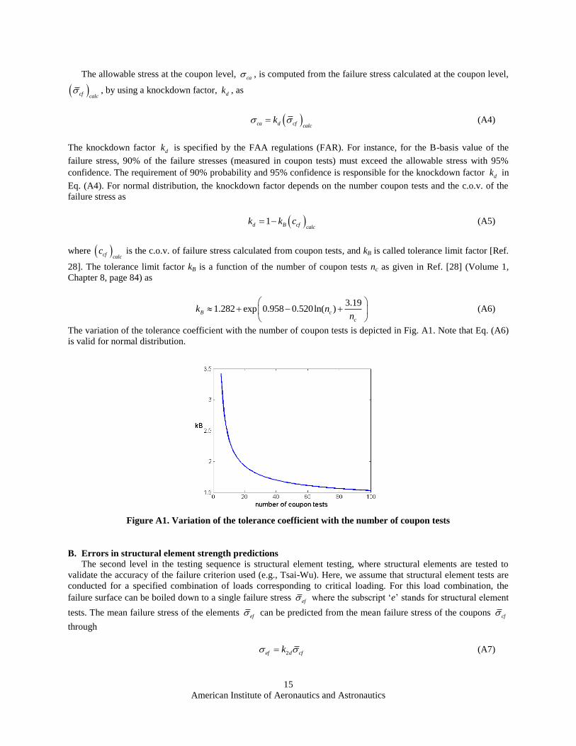
where cf calcc is the c.o.v. of failure stress calculated from coupon tests, and kB is called tolerance limit factor [Ref.
28]. The tolerance limit factor kB is a function of the number of coupon tests nc as given in Ref. [28] (Volume 1,
Chapter 8, page 84) as
3.19
1.282 exp 0.958 0.520ln( )B c
c
k nn
(A6)
The variation of the tolerance coefficient with the number of coupon tests is depicted in Fig. A1. Note that Eq. (A6)
is valid for normal distribution.
Figure A1. Variation of the tolerance coefficient with the number of coupon tests
B. Errors in structural element strength predictions
The second level in the testing sequence is structural element testing, where structural elements are tested to
validate the accuracy of the failure criterion used (e.g., Tsai-Wu). Here, we assume that structural element tests are
conducted for a specified combination of loads corresponding to critical loading. For this load combination, the
failure surface can be boiled down to a single failure stress ef where the subscript „e‟ stands for structural element
tests. The mean failure stress of the elements ef can be predicted from the mean failure stress of the coupons cf
through
2ef d cfk (A7)
American Institute of Aeronautics and Astronautics
16
where 2dk is the ratio between the unidirectional failure stress and the failure stress of a ply in a laminate under
combined loading. If the failure theory used to predict the failure was perfect, and we performed infinite number of
coupon tests, then we could predict 2dk exactly, and the actual value would vary only due to material variability.
However, neither the failure theory is perfect nor infinite tests are performed, so the calculated value of 2dk will be
2 21d ef dcalck e k (A8)
where eef is the error in the failure theory. Note that the sign in front of the error term is negative, since we
consistently formulate the error expressions such that a positive error implies a conservative decision. Then, the
calculated value of the mean failure stress at the element level can be related to the calculated value of the mean
failure stress at the coupon level via
2 21ef d cf ef d cfcalccalc calc calck e k (A9)
Here, we take 2dk = 1 for simplicity. So, we have
1ef ef cfcalc calce (A10)
The initial distribution of ef calc is obtained by estimate of
efe and using the results of coupon tests cf calc . The
information from element tests is used by performing Bayesian procedure to update the failure stress distribution
(see Appendix B for details). In practice, simpler procedures are often used, such as selecting the lowest failure
stress from element tests. Therefore, our assumption will tend to overestimate the beneficial effect of element tests.
If Bayesian updating were used directly within the main MCS loop for design load carrying area determination,
the computational cost would be very high. Instead, Bayesian updating is performed outside from the MCS loop for
a range of possible test results. It is important to note that the error definition used in the Bayesian updating code is
different from the error definition used in the MCS code. In the Bayesian updating code, the error is measured from
the calculated values of the failure stress, ef calc , such that the true and the calculated values of the failure stress
are related through 1ef eftrue calcerror . In the MCS code, on the other hand, the error is measured from
the true value of the failure stress such that the true and the calculated values of the failure stress are related through
1ef ef efcalc truee . Therefore, while the Bayesian updating is implemented, a random error fe generated in
the main MCS code is transferred to 1
11 ef
errore
while running the Bayesian updating code. This
complication reflects the fact that in the MCS loop we consider many possible element analysis and test results,
while the engineer carrying the element tests has a unique set of computations and test results.
The allowable stress based on the element test is calculated from
ea d ef calck (A11)
Here the updated value of the mean failure stress updated
ef calc is used, which corresponds to the most likely value of
the mean failure stress (having the maximum PDF).
Combining Eqs. (A4), (A10) and (A11), we have
1ea ef cae (A12)
American Institute of Aeronautics and Astronautics
17
C. Errors in structural strength predictions
Due to the complexity of the overall structural system, there will be errors in failure prediction of the overall
structure that we denote as fe . If we follow the formulation we used in expressing ef calc
in terms of cf calc ,
the calculated mean failure stress of the overall structure, f calc , can be expressed in terms of the calculated mean
failure stress of the structural element, ef calc , through
1f f efcalc calce (A13)
The allowable stress at the structural design level, a , can be related to the allowable stress computed at the
element level, ea , through the following relation
1a f f eak e (A14)
where fk is an additional knockdown factor used at the structural level as an extra precaution. Here fk is taken
0.95. Combining Eqs. (A12) and (A14), we can obtain
1 1a ef f f ace e k (A15)
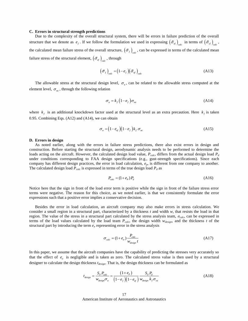
D. Errors in design
As noted earlier, along with the errors in failure stress predictions, there also exist errors in design and
construction. Before starting the structural design, aerodynamic analysis needs to be performed to determine the
loads acting on the aircraft. However, the calculated design load value, Pcalc, differs from the actual design load Pd
under conditions corresponding to FAA design specifications (e.g., gust-strength specifications). Since each
company has different design practices, the error in load calculation, ep, is different from one company to another.
The calculated design load Pcalc is expressed in terms of the true design load Pd as
(1 )calc P dP e P (A16)
Notice here that the sign in front of the load error term is positive while the sign in front of the failure stress error
terms were negative. The reason for this choice, as we noted earlier, is that we consistently formulate the error
expressions such that a positive error implies a conservative decision.
Besides the error in load calculation, an aircraft company may also make errors in stress calculation. We
consider a small region in a structural part, characterized by a thickness t and width w, that resists the load in that
region. The value of the stress in a structural part calculated by the stress analysis team, σcalc, can be expressed in
terms of the load values calculated by the load team Pcalc, the design width wdesign, and the thickness t of the
structural part by introducing the term eσ representing error in the stress analysis
(1 ) calc
calc
design
Pe
w t (A17)
In this paper, we assume that the aircraft companies have the capability of predicting the stresses very accurately so
that the effect of e is negligible and is taken as zero. The calculated stress value is then used by a structural
designer to calculate the design thickness tdesign. That is, the design thickness can be formulated as
1
1 1
PF calc F d
design
design a design f caf ef
eS P S Pt
w w ke e
(A18)
American Institute of Aeronautics and Astronautics
18
Then, the design value of the load carrying area can be expressed as
1
1 1
P F d
design design design
f caf ef
e S PA t w
ke e
(A19)
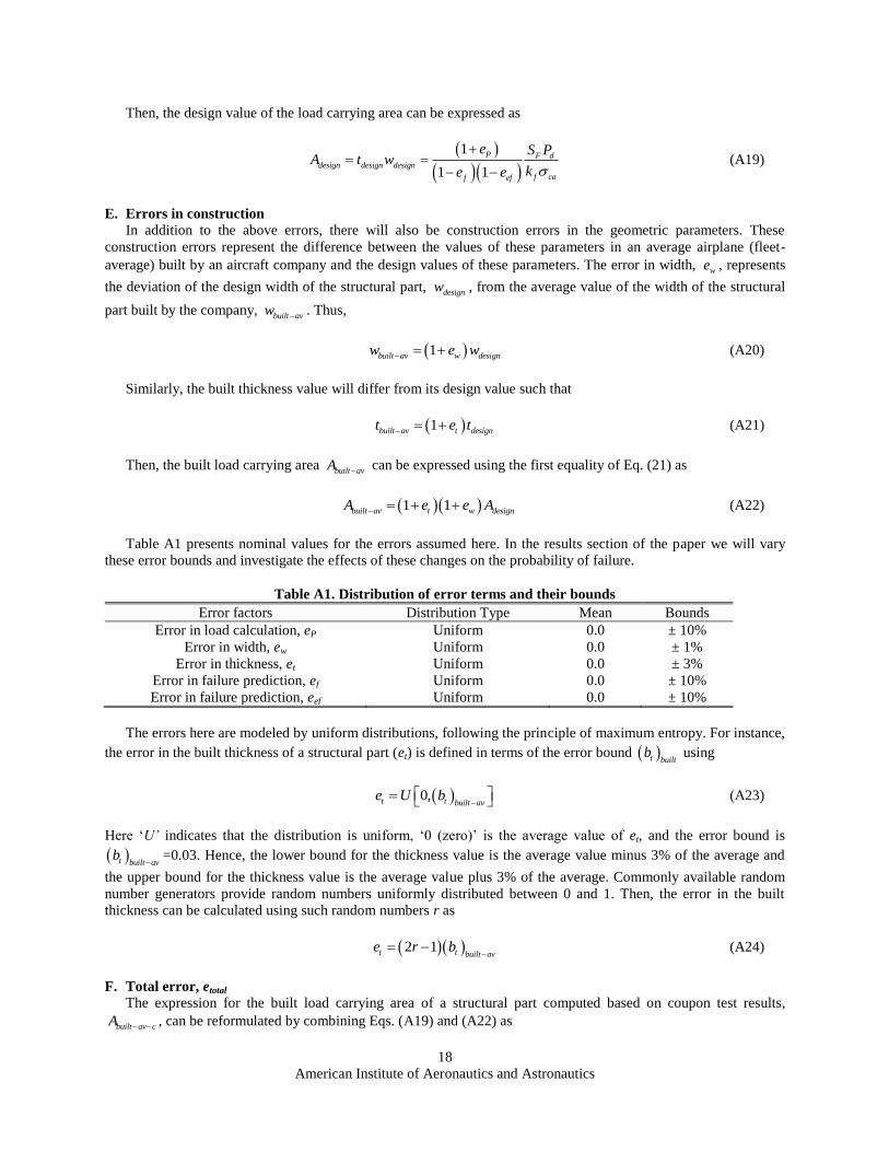
E. Errors in construction
In addition to the above errors, there will also be construction errors in the geometric parameters. These
construction errors represent the difference between the values of these parameters in an average airplane (fleet-
average) built by an aircraft company and the design values of these parameters. The error in width, we , represents
the deviation of the design width of the structural part, designw , from the average value of the width of the structural
part built by the company, built avw
. Thus,
1built av w designw e w (A20)
Similarly, the built thickness value will differ from its design value such that
1built av t designt e t (A21)
Then, the built load carrying area built avA
can be expressed using the first equality of Eq. (21) as
1 1built av t w designA e e A (A22)
Table A1 presents nominal values for the errors assumed here. In the results section of the paper we will vary
these error bounds and investigate the effects of these changes on the probability of failure.
Table A1. Distribution of error terms and their bounds
Error factors Distribution Type Mean Bounds
Error in load calculation, eP Uniform 0.0 ± 10%
Error in width, ew Uniform 0.0 ± 1%
Error in thickness, et Uniform 0.0 ± 3%
Error in failure prediction, ef Uniform 0.0 ± 10%
Error in failure prediction, eef Uniform 0.0 ± 10%
The errors here are modeled by uniform distributions, following the principle of maximum entropy. For instance,
the error in the built thickness of a structural part (et) is defined in terms of the error bound t builtb using
0,t t built ave U b
(A23)
Here „U’ indicates that the distribution is uniform, „0 (zero)‟ is the average value of et, and the error bound is
t built avb
=0.03. Hence, the lower bound for the thickness value is the average value minus 3% of the average and
the upper bound for the thickness value is the average value plus 3% of the average. Commonly available random
number generators provide random numbers uniformly distributed between 0 and 1. Then, the error in the built
thickness can be calculated using such random numbers r as
2 1t t built ave r b
(A24)
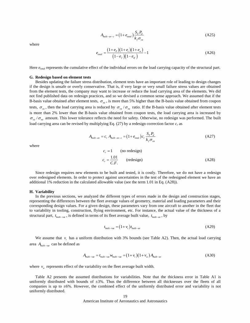
F. Total error, etotal
The expression for the built load carrying area of a structural part computed based on coupon test results,
built av cA , can be reformulated by combining Eqs. (A19) and (A22) as
American Institute of Aeronautics and Astronautics
19
1 F d
built av c total
f ca
S PA e
k (A25)
where
1 1 1
11 1
P t w
total
f ef
e e ee
e e
(A26)
Here etotal represents the cumulative effect of the individual errors on the load carrying capacity of the structural part.
G. Redesign based on element tests
Besides updating the failure stress distribution, element tests have an important role of leading to design changes
if the design is unsafe or overly conservative. That is, if very large or very small failure stress values are obtained
from the element tests, the company may want to increase or reduce the load carrying area of the elements. We did
not find published data on redesign practices, and so we devised a common sense approach. We assumed that if the
B-basis value obtained after element tests, ea , is more than 5% higher than the B-basis value obtained from coupon
tests, ca , then the load carrying area is reduced by /ca ea ratio. If the B-basis value obtained after element tests
is more than 2% lower than the B-basis value obtained from coupon tests, the load carrying area is increased by
/ca ea amount. This lower tolerance reflects the need for safety. Otherwise, no redesign was performed. The built
load carrying area can be revised by multiplying Eq. (27) by a redesign correction factor cr as
1 F d
built av r built av c total r
f ca
S PA c A e c
k (A27)
where
1rc (no redesign)
1.01
. .rc
C F (redesign) (A28)
Since redesign requires new elements to be built and tested, it is costly. Therefore, we do not have a redesign
over redesigned elements. In order to protect against uncertainties in the test of the redesigned element we have an
additional 1% reduction in the calculated allowable value (see the term 1.01 in Eq. (A28)).
H. Variability
In the previous sections, we analyzed the different types of errors made in the design and construction stages,
representing the differences between the fleet average values of geometry, material and loading parameters and their
corresponding design values. For a given design, these parameters vary from one aircraft to another in the fleet due
to variability in tooling, construction, flying environment, etc. For instance, the actual value of the thickness of a
structural part, varbuiltt , is defined in terms of its fleet average built value, built avt , by
var 1built t built avt v t (A29)
We assume that tv has a uniform distribution with 3% bounds (see Table A2). Then, the actual load carrying
area varbuiltA
can be defined as
var var var 1 1built built built t w built avA t w v v A (A30)
where wv represents effect of the variability on the fleet average built width.
Table A2 presents the assumed distributions for variabilities. Note that the thickness error in Table A1 is
uniformly distributed with bounds of ±3%. Thus the difference between all thicknesses over the fleets of all
companies is up to ±6%. However, the combined effect of the uniformly distributed error and variability is not
uniformly distributed.
American Institute of Aeronautics and Astronautics
20
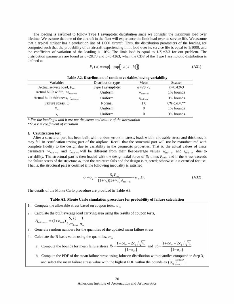
The loading is assumed to follow Type I asymptotic distribution since we consider the maximum load over
lifetime. We assume that one of the aircraft in the fleet will experience the limit load over its service life. We assume
that a typical airliner has a production line of 1,000 aircraft. Thus, the distribution parameters of the loading are
computed such that the probability of an aircraft experiencing limit load over its service life is equal to 1/1000, and
the coefficient of variation of the loading is 10%. The limit load is equal to 1/SF=2/3 for our problem. The
distribution parameters are found as a=28.73 and b=0.4263, when the CDF of the Type I asymptotic distribution is
defined as
exp expXF x a x b (A31)
Table A2. Distribution of random variables having variability
Variables Distribution type Mean Scatter
Actual service load, Pact Type I asymptotic a=28.73 b=0.4263
Actual built width, varbuiltw
Uniform built avw 1% bounds
Actual built thickness, varbuiltt
Uniform built avt 3% bounds
Failure stress, σf Normal 1.0 8% c.o.v.**
wv Uniform 0 1% bounds
tv Uniform 0 3% bounds
* For the loading a and b are not the mean and scatter of the distribution
**c.o.v.= coefficient of variation
I. Certification test
After a structural part has been built with random errors in stress, load, width, allowable stress and thickness, it
may fail in certification testing part of the airplane. Recall that the structural part will not be manufactured with
complete fidelity to the design due to variability in the geometric properties. That is, the actual values of these
parameters varbuiltw
and varbuiltt
will be different from their fleet-average values built avw
and built avt
due to
variability. The structural part is then loaded with the design axial force of SF times Pcalc, and if the stress exceeds
the failure stress of the structure σf, then the structure fails and the design is rejected; otherwise it is certified for use.
That is, the structural part is certified if the following inequality is satisfied
01 1
F calc
f f
t w built av
S P
v v A
(A32)
The details of the Monte Carlo procedure are provided in Table A3.
Table A3. Monte Carlo simulation procedure for probability of failure calculation
1. Compute the allowable stress based on coupon tests, ca
2. Calculate the built average load carrying area using the results of coupon tests,
1(1 ) F d
built av c total
f design ca
S PA e
k w
3. Generate random numbers for the quantiles of the updated mean failure stress
4. Calculate the B-basis value using the quantiles, ea
a. Compute the bounds for mean failure stress
1 2
1
ef f c
ef
be c nlb
e
and
1 2
1
ef f c
ef
be c nub
e
b. Compute the PDF of the mean failure stress using Johnson distribution with quantiles computed in Step 3,
and select the mean failure stress value with the highest PDF within the bounds as updated
ef calc .
American Institute of Aeronautics and Astronautics
21
c. Compute B-basis value, 1updated
ea B cf efcalc calck c
5. Compute a correction factor for the B-basis value, ea
ca
CF
. Limit the value of CF to [0.9, 1.1].
That is, if CF < 0.9, then CF = 0.9. If CF > 1.1, then CF = 1.1.
6. Revise the built average load carrying area based on the value of CF.
a. If 0.98CF , then redesign is needed, we will increase the load carrying area by CF. Hence, the new load
carrying area is 1.01
built av built av cA ACF
. Here the factor 1.01 is used to avoid a second redesign of
elements.
b. If 0.98 1.05CF , then no redesign is needed. So, the load carrying area is built av built av cA A .
c. If 1.05CF , then redesign is needed, we will decrease the load carrying area by CF. Hence, the new load
carrying area is 1.01
built av built av cA ACF
. Here again the factor 1.01 is used to avoid a second redesign of
elements.
7. Using built avA
, compute the probability of failure in service (Pf), and probability of failure in certification test
(PFCT).
Appendix B: Bayesian updating of the failure stress distribution from the results of element tests
The initial distribution of the element failure stress is obtained by using a failure criterion (e.g., Tsai-Wu theory)
using the results of coupon tests. There will be two sources of error in this prediction. First, since a finite number of
coupon tests are performed, the mean and standard deviation of the failure stress obtained through the coupon tests
will be different from the actual mean and standard deviation.
We consider a typical situation relating to updating analytical predictions of strength based on tests. We assume
that the analytical prediction of the failure stress of a structural element, efcalc
, applies to the average failure
stress eftrue
of an infinite number of nominally identical structural elements. The error eef of our analytical
prediction is defined by
1ef ef eftrue calc
e (B1)
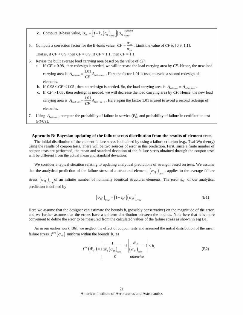
Here we assume that the designer can estimate the bounds be (possibly conservative) on the magnitude of the error,
and we further assume that the errors have a uniform distribution between the bounds. Note here that it is more
convenient to define the error to be measured from the calculated values of the failure stress as shown in Fig B1.
As in our earlier work [36], we neglect the effect of coupon tests and assumed the initial distribution of the mean
failure stress ini
eff uniform within the bounds eb as
1
if 12
0
ef
eini
ef e ef efcalc calc
bf b
othewise
(B2)
American Institute of Aeronautics and Astronautics
22
Figure B1: Error and variability in failure stress. The error is centered around the computed value, and is
assumed to be uniformly distributed here. The variability distribution, on the other hand, is lognormal with mean
equal to the true average failure stress.
Then, the distribution of the mean failure stress is updated using the Bayesian updating with a given 1,f test
as
1,
1,
ini
test ef efupd
ef
ini
test ef ef ef
f ff
f f d
(B3)
where 1, 1,; ,test ef ef f eftest
f Normal Std is the likelihood function reflecting possible variability of the
first test result 1,ef test
. Note that 1,test eff is not a probability distribution in ef ; it is the conditional probability
density of obtaining test result 1,ef test
, given that the mean value of the failure stress is ef . Subsequent tests are
handled by the same equations, using the updated distribution, as the initial one.
If the Bayesian updating procedure defined above is used directly within an MCS loop for design load carrying
area determination, the computational cost will be very high. In this paper, instead, the Bayesian updating is
performed aside from the MCS loop. In this separate loop, we first simulate the coupon tests by drawing random
samples for the mean and standard deviation of the calculated failure stress cf and cfStd . Then, we simulate ne
number of element tests, ef test . The element test results along with the mean and the standard deviation are used
to define the likelihood function as 1, 1,; ,test ef ef cf cftest
f Normal Std in Eq. (B3). The initial
distribution ini
eff in Eq. (B3) is uniformly distributed within some bounds as given in Eq. (B4).
1
if 12
0
ef
eini
ef e cf cf
bf b
othewise
(B4)
We found that applying the error bounds eb before the Bayesian updating or after the updating do not matter.
Applying the error bounds before Bayesian updating means calculating the initial distribution ini
eff from Eq.
(B4) and then using Eq. (B3). To apply the error bounds after the Bayesian updating, however, we first assume very
ftrue
fcalc
f ftest true
fv
fe
( )ff v
( )ff e
f
Probability density
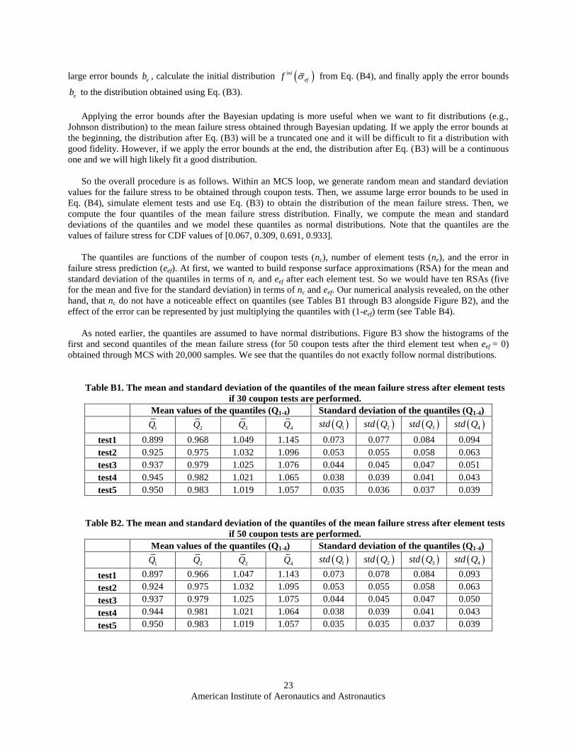
American Institute of Aeronautics and Astronautics
23
large error bounds eb , calculate the initial distribution ini
eff from Eq. (B4), and finally apply the error bounds
eb to the distribution obtained using Eq. (B3).
Applying the error bounds after the Bayesian updating is more useful when we want to fit distributions (e.g.,
Johnson distribution) to the mean failure stress obtained through Bayesian updating. If we apply the error bounds at
the beginning, the distribution after Eq. (B3) will be a truncated one and it will be difficult to fit a distribution with
good fidelity. However, if we apply the error bounds at the end, the distribution after Eq. (B3) will be a continuous
one and we will high likely fit a good distribution.
So the overall procedure is as follows. Within an MCS loop, we generate random mean and standard deviation
values for the failure stress to be obtained through coupon tests. Then, we assume large error bounds to be used in
Eq. (B4), simulate element tests and use Eq. (B3) to obtain the distribution of the mean failure stress. Then, we
compute the four quantiles of the mean failure stress distribution. Finally, we compute the mean and standard
deviations of the quantiles and we model these quantiles as normal distributions. Note that the quantiles are the
values of failure stress for CDF values of [0.067, 0.309, 0.691, 0.933].
The quantiles are functions of the number of coupon tests (nc), number of element tests (ne), and the error in
failure stress prediction (eef). At first, we wanted to build response surface approximations (RSA) for the mean and
standard deviation of the quantiles in terms of nc and eef after each element test. So we would have ten RSAs (five
for the mean and five for the standard deviation) in terms of nc and eef. Our numerical analysis revealed, on the other
hand, that nc do not have a noticeable effect on quantiles (see Tables B1 through B3 alongside Figure B2), and the
effect of the error can be represented by just multiplying the quantiles with (1-eef) term (see Table B4).
As noted earlier, the quantiles are assumed to have normal distributions. Figure B3 show the histograms of the
first and second quantiles of the mean failure stress (for 50 coupon tests after the third element test when eef = 0)
obtained through MCS with 20,000 samples. We see that the quantiles do not exactly follow normal distributions.
Table B1. The mean and standard deviation of the quantiles of the mean failure stress after element tests
if 30 coupon tests are performed.
Mean values of the quantiles (Q1-4) Standard deviation of the quantiles (Q1-4)
1Q 2Q
3Q 4Q 1std Q 2std Q 3std Q 4std Q
test1 0.899 0.968 1.049 1.145 0.073 0.077 0.084 0.094
test2 0.925 0.975 1.032 1.096 0.053 0.055 0.058 0.063
test3 0.937 0.979 1.025 1.076 0.044 0.045 0.047 0.051
test4 0.945 0.982 1.021 1.065 0.038 0.039 0.041 0.043
test5 0.950 0.983 1.019 1.057 0.035 0.036 0.037 0.039
Table B2. The mean and standard deviation of the quantiles of the mean failure stress after element tests
if 50 coupon tests are performed.
Mean values of the quantiles (Q1-4) Standard deviation of the quantiles (Q1-4)
1Q 2Q
3Q 4Q 1std Q 2std Q 3std Q 4std Q
test1 0.897 0.966 1.047 1.143 0.073 0.078 0.084 0.093
test2 0.924 0.975 1.032 1.095 0.053 0.055 0.058 0.063
test3 0.937 0.979 1.025 1.075 0.044 0.045 0.047 0.050
test4 0.944 0.981 1.021 1.064 0.038 0.039 0.041 0.043
test5 0.950 0.983 1.019 1.057 0.035 0.035 0.037 0.039
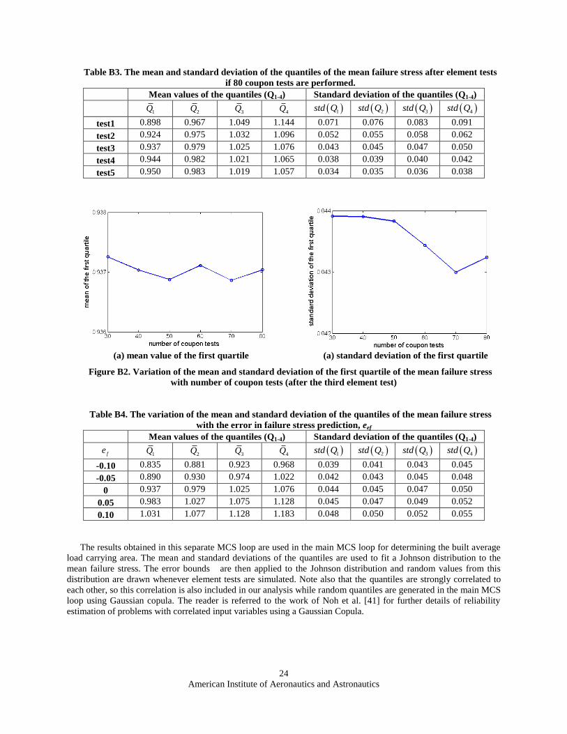
American Institute of Aeronautics and Astronautics
24
Table B3. The mean and standard deviation of the quantiles of the mean failure stress after element tests
if 80 coupon tests are performed.
Mean values of the quantiles (Q1-4) Standard deviation of the quantiles (Q1-4)
1Q 2Q
3Q 4Q 1std Q 2std Q 3std Q 4std Q
test1 0.898 0.967 1.049 1.144 0.071 0.076 0.083 0.091
test2 0.924 0.975 1.032 1.096 0.052 0.055 0.058 0.062
test3 0.937 0.979 1.025 1.076 0.043 0.045 0.047 0.050
test4 0.944 0.982 1.021 1.065 0.038 0.039 0.040 0.042
test5 0.950 0.983 1.019 1.057 0.034 0.035 0.036 0.038
(a) mean value of the first quartile (a) standard deviation of the first quartile
Figure B2. Variation of the mean and standard deviation of the first quartile of the mean failure stress
with number of coupon tests (after the third element test)
Table B4. The variation of the mean and standard deviation of the quantiles of the mean failure stress
with the error in failure stress prediction, eef
Mean values of the quantiles (Q1-4) Standard deviation of the quantiles (Q1-4)
fe 1Q
2Q 3Q
4Q 1std Q 2std Q 3std Q 4std Q
-0.10 0.835 0.881 0.923 0.968 0.039 0.041 0.043 0.045
-0.05 0.890 0.930 0.974 1.022 0.042 0.043 0.045 0.048
0 0.937 0.979 1.025 1.076 0.044 0.045 0.047 0.050
0.05 0.983 1.027 1.075 1.128 0.045 0.047 0.049 0.052
0.10 1.031 1.077 1.128 1.183 0.048 0.050 0.052 0.055
The results obtained in this separate MCS loop are used in the main MCS loop for determining the built average
load carrying area. The mean and standard deviations of the quantiles are used to fit a Johnson distribution to the
mean failure stress. The error bounds are then applied to the Johnson distribution and random values from this
distribution are drawn whenever element tests are simulated. Note also that the quantiles are strongly correlated to
each other, so this correlation is also included in our analysis while random quantiles are generated in the main MCS
loop using Gaussian copula. The reader is referred to the work of Noh et al. [41] for further details of reliability
estimation of problems with correlated input variables using a Gaussian Copula.
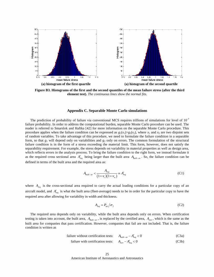
American Institute of Aeronautics and Astronautics
25
(a) histogram of the first quartile (a) histogram of the second quartile
Figure B3. Histograms of the first and the second quantiles of the mean failure stress (after the third
element test). The continuous lines show the normal fits.
Appendix C. Separable Monte Carlo simulations
The prediction of probability of failure via conventional MCS requires trillions of simulations for level of 10-7
failure probability. In order to address the computational burden, separable Monte Carlo procedure can be used. The
reader is referred to Smarslok and Haftka [42] for more information on the separable Monte Carlo procedure. This
procedure applies when the failure condition can be expressed as g1(x1)>g2(x2), where x1 and x2 are two disjoint sets
of random variables. To take advantage of this procedure, we need to formulate the failure condition in a separable
form, so that g1 will depend only on variabilities and g2 only on errors. The common formulation of the structural
failure condition is in the form of a stress exceeding the material limit. This form, however, does not satisfy the
separability requirement. For example, the stress depends on variability in material properties as well as design area,
which reflects errors in the analysis process. To bring the failure condition to the right form, we instead formulate it
as the required cross sectional area reqA being larger than the built area built avA
. So, the failure condition can be
defined in terms of the built area and the required area as:
1 1
req
built av req
t w
AA A
v v
(C1)
where reqA is the cross-sectional area required to carry the actual loading conditions for a particular copy of an
aircraft model, and reqA is what the built area (fleet-average) needs to be in order for the particular copy to have the
required area after allowing for variability in width and thickness.
req act fA P (C2)
The required area depends only on variability, while the built area depends only on errors. When certification
testing is taken into account, the built area, built avA , is replaced by the certified area, certA , which is the same as the
built area for companies that pass certification. However, companies that fail are not included. That is, the failure
condition is written as
failure without certification tests: 0built av reqA A (C3a)
failure with certification tests: 0cert reqA A (C3b)
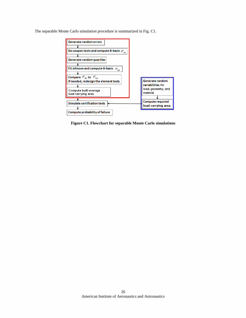
American Institute of Aeronautics and Astronautics
26
The separable Monte Carlo simulation procedure is summarized in Fig. C1.
Figure C1. Flowchart for separable Monte Carlo simulations