SOILS, SEC 5 • SOIL AND LANDSCAPE ECOLOGY • RESEARCH ARTICLE

Relationship between soil depth and terrain attributes in karstregion in Southwest China

Qiyong Yang & Fawang Zhang & Zhongcheng Jiang &

Wenjun Li & Jianbing Zhang & Faming Zeng & Hui Li

Received: 27 December 2013 /Accepted: 19 April 2014# Springer-Verlag Berlin Heidelberg 2014

AbstractPurpose Soil depth generally varies in peak-cluster depres-sion regions in rather complex ways. Because conventionalsoil survey methods in these regions require a considerableamount of time, effort, and consequently relatively large bud-get, new methods are required in karst regions.Materials and methods This study explored the relationshipbetween soil depth and terrain attributes abstracted from dig-ital elevation models (DEMs) at different spatial resolutions inthe Guohua Karst Ecological Experimental Area, a represen-tative region of peak-cluster depression in Southwest China. Auniform 140 m×140 m grid combined with representativehillslope methodology was used to select 171 sampling pointswhere soil depth was measured. Nine primary and secondaryterrain attributes, such as elevation, slope, aspect, especialcatchment area, wetness index, length-slope factor, streampower index, relief degree of land surface, and distance from

ridge of mountains, were computed from DEMs at differentspatial resolutions. The optimal DEM spatial resolution wasdetermined by Grey relational analysis (GRA) to reflect thecorrelations between soil depth and terrain attributes.Results and discussion GRA revealed that the 10-m spatialresolution DEM can best reflect the relationship between soildepth and terrain attributes; therefore, the terrain attributes atthis resolution were used for multiple linear stepwise regres-sion (MLSR) analysis. The result of MLSR indicated thatslope, TWI, and elevation could explain about 61.4 % of thetotal variability in soil depth in the study area.Conclusions The terrain attributes of slope, WTI and eleva-tion can be used to evaluate soil depth in this region very well.This proposed approach may be applicable to other peak-cluster depression regions in the karst areas at a larger scale.

Keywords Digital elevationmodel .Peak-clusterdepression .

Soil depth . Spatial resolution . Terrain attribute

1 Introduction

Regolith depth, often referred to by geomorphologists andengineers as soil depth, is defined as the depth from thesurface to more-or-less consolidated material (Kuriakoseet al. 2009; Mehnatkesh et al. 2013). Soil depth in manylandscapes affects vegetation growth (Fuhlendorf andSmeins 1998; Meyer et al. 2007; Hirzel and Matus 2013;Liang and Uchida 2014) and hydromechanical responses(DeRose et al. 1991; Bertoldi et al. 2004; Wang et al. 2006;Lanni et al. 2012). In karst regions, soil depth is also definedas one of the crucial indicators used to assess karst rockydesertification (KRD). Soil erosion results in a decrease insoil depth, which is always accelerated under the impacts ofintense human activities in vulnerable environments and inkarst areas. In karst areas, KRD is a process in which soil is

Responsible editor: Claudio Bini

Q. Yang (*) : F. Zhang (*) : Z. Jiang : F. ZengKey Laboratory of Karst Ecosystem and Treatment of RockyDesertification, Institute of Karst Geology, Chinese Academy ofGeological Sciences, Guilin 541004, Chinae-mail: yangqiyong0739@163.come-mail: zhangfawang@karst.ac.cn

J. ZhangKey Laboratory of Beibu Gulf Environment Change and ResourcesUse, Ministry of Education (Guangxi Teachers EducationUniversity), Nanning 530001, China

W. LiCollege of Resources and Environment and Tourism, HunanUniversity of Arts and Science, Changde 415000, China

H. LiCollege of Environment and Resources, Guangxi Normal University,541004 Guilin, China

J Soils SedimentsDOI 10.1007/s11368-014-0904-6

seriously or even thoroughly eroded, to the point that bedrockis widely exposed and land productivity declines seriously;ultimately, the landscape appears similar to desert (Yuan 1993;Cai 1997; Huang and Cai 2006; Xiong et al. 2008; Zhang et al.2011). When KRD occurs, soil depth decreases, which seri-ously threatens soil quality and productivity in the karst re-gions of Southwest China. The type of vegetation found inKRD regions is principally controlled by soil water storagecapacity and therefore soil depth. Therefore, studying soildepth in karst regions as part of the assessment of rockydesertification and ecological restoration has practicalsignificance.

Many different factors, including elevation, slope, curva-ture, parent material, climate, upslope conditions, vegetationcover, and land use, influence soil depth (Minasny andMcBratney 1999; Kuriakose et al. 2009; Ziadat 2010;Mehnatkesh et al. 2013). Soil scientists have identified terrain,including soil depth, as one of the pedogenic factors(Florinsky et al. 2002; Pei et al. 2010; Mehnatkesh et al.2013) that significantly influence the spatial distribution ofvarious soil properties. Boer et al. (1996) reported on theapplication of terrain attributes to mapping soil depth classesat high resolution over large areas under dry Mediterraneanconditions. Hengl et al. (2004) compared the spatial predictionquality of various soil properties using six topographical var-iables and nine soil mapping units. Penížek and Borůvka(2006) compared several geostatistical methods forpredicting soil depth and concluded that cokriging withslope yielded better results than ordinary kriging, regressionkriging, and linear regression. Kuriakose et al. (2009)compared four methods for the spatial prediction of soildepth using five terrain variables and land use types. Ziadat(2010) investigated the possibility of predicting soil depthusing some terrain attributes derived from digital elevationmodels (DEMs) with geographic information systems andsuggested an approach that can be used to predict other soil

attributes. Wang et al. (2011) used fuzzy c-means clusteringbased on the relationships between soil depth and landscapeparameters, i.e., elevation, slope, planform curvature, profilecurvature, runoff intensity, and a topographical wetness index,to predict soil depth of the west Tiaoxi catchment in China.These results suggested that terrain attributes, such as slope,wetness index, mean curvature, and a stream power index, arevaluable auxiliary variables that have proved useful forpredicting soil depth.

The prediction of soil properties by terrain attributesmainlydepends on how significant the correlations are between soilproperties and terrain attributes. However, the correlationsmay vary with different spatial resolutions of DEM, particu-larly in complex terrain areas, such as peak-cluster depres-sions. Many research studies on the relationship betweenspatial resolution and terrain attributions have been conducted(Wu et al. 2008; Liu et al. 2011), but little attention has beenpaid to the effects of the spatial resolution of a DEM whenterrain attributes are used to predict soil properties. The ob-jectives of this work are (a) to evaluate the relationship be-tween the soil depth and terrain attributes and to select theoptimal spatial resolution of DEM in peak-cluster depressionsand (b) to determine the most successful multiple linear step-wise regressions (MLSR) model for soil depth mapping in thestudy area.

2 Materials and methods

2.1 Study area

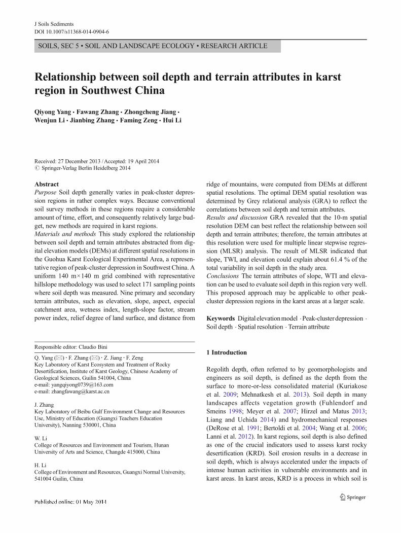
The Guohua Karst Ecological Experimental Area, located inPingguo County, Southwest China, covers a total area of10 km2 and was selected as the study area (116° 41′–117°30′ E, 40° 14′–40° 48′ N) (Fig. 1). The typical karst peak-cluster depression landscape (a combination of clustered

Fig. 1 Location of Guohua KarstEcological Experimental Areaand distribution of soil depth (cm)sampling site training and testdata

J Soils Sediments

peaks with a common base) ranges from 120 to 560 m abovethe mean sea level in elevation. The humid subtropicalmonsoon climate has a mean annual temperature of 13–14 °C and abundant but seasonally uneven rainfall. Theannual mean precipitation (1958 to 2006) was 1,331 mm,but over 86 % of this falls during the rainy season (April–October). Various types of natural vegetation occur in thestudy area, dominated by evergreen broad-leaved forest anddeciduous broad-leaved forest. The generally thin karst soilis unevenly distributed because soil formation occurs slow-ly and varies widely across the terrain. Soil types includemainly calcareous, yellow, and red soils, with calcareoussoil covering 87.3 % of the study area. Five land usecategories occur in the study area: forest land, grassland,cultivated land, water bodies, and urbanized areas (towns,roads, and other urbanized areas). Cultivated land includesdry and paddy land. In the past, KRD seriously impactedthe area but the “Green for Grain” program was initiated inSouthwest China to protect the fragile karst environment.Forests in hilly areas have been effectively managed andprotected, and illegal wood cutting has been restrained. Thevegetation has been partly restored, and KRD has beenrelieved.

2.2 Field work and soil depth measurements

The field work was conducted in August 2012, and 149sites were measured in the study area using a regular140 m×140 m grid. Because of the variable terrain inthe studied area, four representative hillslopes were cho-sen and 22 additional sites were measured using ran-domly stratified methodology, considering all geomor-phic surfaces including summit, shoulder, backslope,footslope, toeslope, and depression. A global positioningsystem (Juno ST, Trimble Navigation, Ltd., Sunnyvale,CA, USA) recorded the locations of the sampling sites.Overall, 171 auger holes were made by the knockingpole method (Uchida et al. 2008; Kuriakose et al.2009); an iron spear was pierced into the soil untilbedrock was reached.

All data were subjected to exploratory analyses by produc-ing boxplots and Paūta Criterion to remove outliers (Zhangand Yuan 1997). In this study, no outliers were removedthrough the exploratory analyses. The soil sample data weredivided into a training (interpolation) data set, which was usedfor the models used to predict soil depth, and test (validation)data, which were used to validate the models; the latter repre-sented about 20 % of the entire set of data (Fig. 1). Thetraining data and the test data were automatically generatedin ArcGIS software, using the Geostatistical Analystextension.

2.3 Terrain analysis

A contour map for the study area was obtained from a1:10,000 scale topographic map and the data were thentransferred to a Triangulated Irregular Network map. Rasterformat DEMs of spatial resolutions of 5, 10, 15, 20, and 25 mwere derived from the Triangulated Irregular Network map.

Table 1 Definitions of terrain attributes (Moore and Hutchinson 1991;Florinsky et al. 2002; Basso 2005; Pei et al. 2010)

Variable Definition

Primary terrain attributes

(1) Elevation(h, m)

Elevation above mean sea level.

(2) Slope (β,degrees, 0-90°)

Maximum rate of change in elevation from eachDEM cell. It is the gradient at a specified point,and is used to identify the steepest of thegradients between a point and its neighbors.It shows the velocity of substance flows.β ¼ arctan

ffiffiffiffiffiffiffiffiffiffiffiffiffiffiffiffiffip2 þ q2a

p

(3) Aspect angle(α, °)

Aspect is the direction of gradient, directing themaximum rate of change in the elevation fromeach cell DEM. It shows the direction ofsubstance flows. Counter-clockwise from east;90° to the north, 180° to the west, 270° to the

south, and 360° to the east. α ¼ arctan qp

� �a

Secondary terrain attributes

(4) Especialcatchment area(As, m2 m−1)

Upslope area per unit width of contour, and it isratio of an area of an exclusive figure formed by acontour intercept with a given point on the landsurface and is a measure of thecontributing area.

(5) Wetnessindex (WTI)

Sets catchment area in relation to the slope gradient.It has been used to characterize the spatialdistribution of zones of surface saturation andsoil water content in landscapes. It shows theextent of flow accumulation, which is a wellstudied indicator of soil property and soilmoisture distribution at different landscape

positions. WTI ¼ ln Astanβ

� �

(6) Length-slopefactor (LS)

Length-slope factor (LS) is an important factor ofthe universal soil loss equation (USLE), which issuitable for identifying erosion processes.

LS ¼ As22:13

� �0:6 sinβ0:0896

� �1:3(7) The streampower index(SPI)

SPI is indicative of runoff erosion potential. SPI=ln(100×As×tanβ)

(8) Relief degreeof land surface(RDLS)

RDLS is an important factor in describing thelandform macroscopically

(9) Distancefrom ridge ofmountains(DRM)

DRM describes the horizon distance to mountainridge.

J Soils Sediments

These processions were finished using the Geostatistical 3DAnalyst extension of ArcGIS9.2. Specifically, nine terrainattributes were derived from the DEMs of different spatialresolutions, including primary and secondary terrain attributes(Table 1). All attributes listed in Table 1 were calculated usingArcGIS 9.2.

2.4 Statistical analysis

Descriptive statistics of the experimental data includingmean, minimum, maximum, standard deviation (SD),coefficient of variance (CV), skewness, and kurtosiswere determined using SPSS13.0 software (IBMCom., Chicago, IL, USA). Correlation coefficients usedto define the relationship between soil depth and ter-rain attributes were calculated using SPSS software, aswas the analysis of variance using Duncan’s test. Greyrelational analysis (GRA) was used to determine thebest spatial resolution DEM used to reflect the rela-tionship between soil depth and terrain attributes. TheSPSS software was used for developing multiple linearstepwise regression models on the best spatial resolu-tion DEM. Terrain attributes and soil depth were se-lected as the independent and dependent variables inthe model, respectively.

2.4.1 Grey relational analysis

GRA is a method of measuring the degree of approximationamong sequences according to the grey relational grade. Therelationship among various factors is usually unclear in acomplex multivariate system. Such systems are often referredto as “grey,” implying they contain poor, incomplete, anduncertain information. GRA is an impacting measurementmethod in grey system theory that analyzes uncertain relation-ships between one main factor (parent sequence) and all theother factors (subsequence) in a given system. The theories ofgrey relational analysis have attracted considerable interestamong researchers (Lo 2002; Lin and Ho 2003; Fung 2003;Yang et al. 2010; Palanikumar et al. 2012). The steps used toestablish GRA are listed below:

1. Define the parent sequence and the subsequence.The two sequences, X0 and Xi, with the same

length represent the parent sequence and the subse-quence, respectively, as shown in Eqs. 1 and 2:

X 00 ¼ X 0

0 1ð Þ;X 00 2ð Þ;⋯;X 0

0 nð Þ� � ð1Þ

X 0i ¼ X 0

i 1ð Þ;X 0i 2ð Þ;⋯;X 0

i nð Þ� � ð2Þ

2. Normalize the original sequence.The evaluation indices in the decision matrix

cannot be compared directly because they have dif-ferent dimensions and magnitudes. Therefore, nor-malization is necessary to transfer an original se-quence to a comparable sequence.

In the subsequence, when a larger value of theindex is considered better than a small value, theoriginal sequence can be normalized as shown inEq. 3:

X *0 ¼

X 0i kð Þ−minX 0

i kð ÞmaxX 0

i kð Þ−minX 0i kð Þ ð3Þ

where i=1,…,m; k=1,…, n. m is the number of experimentaldata items and n is the number of parameters. Xi

0(k) denotesthe original sequence, Xi

∗(k) denotes the sequence after thedata preprocessing, maxXi

0(k) denotes the largest value ofXi0(k), minXi

0(k) denotes the smallest value of Xi0(k), and X0

∗

is the desired value.When a smaller value of the index is considered better, the

original sequence can be normalized using Eq. 4:

X *0 ¼

maxX 0i kð Þ−X 0

i kð ÞmaxX 0

i kð Þ−minX 0i kð Þ ð4Þ

3. Calculate the grey relation coefficient using Eq. 5:

εij kð Þ ¼min1≤ i≤m

min1≤ j≤n

X *i kð Þ−X *

0 kð Þ�� ��þ βmax1≤ i≤m

max1≤ j≤n

X *i kð Þ−X *

0 kð Þ�� ��X *

i kð Þ−X *0 kð Þ�� ��þ βmax

1≤ i≤mmax1≤ j≤n

X *i kð Þ−X *

0 kð Þ�� �� ð5Þ

where εij(k) is the grey relational coefficient between the ithindex of the jth project to be evaluated and the ith element ofthe reference sequence; |Xi

∗(k)−X0∗(k)| is the absolute differ-

ence between Xi∗(k) and X0

∗(k); min1 ≤ i ≤m

min1 ≤ j ≤ n

X�i kð Þ−X �

0 kð Þ���

��� and

max1 ≤ i ≤m

max1 ≤ j ≤ n

X�i kð Þ−X �

0 kð Þ���

��� denote the minimum and maximum

absolute difference between Xi∗(k) and X0

∗(k); and β is the

distinguishing coefficient, which is between 0 and 1, and isusually 0.5.

J Soils Sediments

4. Calculate the grey relational degree.After the grey relational coefficient is derived, the

average value of the grey relational coefficients is usuallyconsidered the grey relational grade. The grey relationalgrade (γi) is defined using Eq. 6:

γi ¼1

n

Xk¼1

n

εij kð Þ ð6Þ

5 Sort out relational order.To accurately evaluate and sort out the relational degree

of each subsequence with respect to the parent sequence, itis necessary to put the relational degree in order accordingto magnitude; this order is called the relational order. Thisorder clarifies and sorts out the “priority” and “superiority”of each subsequence with respect to the parent sequence.

2.4.2 Soil depth validation by multiple linear stepwiseregression

In this study, 171 sampling sites were divided into data sets;80 and 20 % for modeling and validation processes, respec-tively. The data sets for modeling and validation processeswere selected randomly at different points on the landscape inthe field to avoid biases in estimation. Terrain attributes wereselected as the independent variables and soil depth wasemployed as the dependent variable in the model. Multiplelinear regression models were developed with SPSS software.

Multiple linear stepwise regressions were used to predictthe spatial variation of soil depth with 137 sampling sites. Themodel was validated with 34 sampling sites. The modelingefficiency (MEF) (Vereecken et al. 1991; Foereid and Høgh-Jensen 2004) and root-mean-square error (RMSE) were usedto validate the performance of the model (Odeh et al. 1995):

MEF ¼ 1−

Xi¼1

n

Oi−Pið Þ2

Xi¼1

n

Oi−O� �2

ð7Þ

RMSE ¼ffiffiffiffiffiffiffiffiffiffiffiffiffiffiffiffiffiffiffiffiffiffiffiffiffiffiffiffiffiffi1

n

Xj¼1

n

Oi−Pið Þ2vuut ð8Þ

where Oi is the observed value and Pi is the correspondingpredicted value. Ois the mean of all observations. The datasetused for validation contained 20 % of the observations.

3 Results and discussion

3.1 Descriptive statistical analysis of soil depth

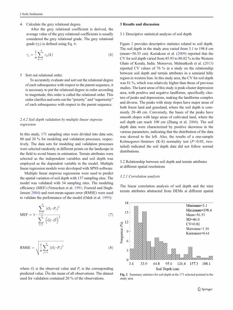
Figure 2 provides descriptive statistics related to soil depth.The soil depth in the study area varied from 3.1 to 198.4 cm(mean=56.53 cm). Kuriakose et al. (2009) reported that theCV for soil depth varied from 45.93 to 80.82 % in theWesternGhats of Kerala, India. Moreover, Mehnatkesh et al. (2013)reported CV values of 76 % in a study on the relationshipbetween soil depth and terrain attributes in a semiarid hillyregion in western Iran. In this study area, the CV for soil depthwas 81 %, which was relatively higher than those of previousstudies. The karst areas of this study is peak-cluster depressionarea, with positive and negative landforms, specifically clus-ters of peaks and depressions, making the landforms complexand diverse. The peaks with steep slopes have major areas ofboth forest land and grassland, where the soil depth is com-monly 20–40 cm. Conversely, the bases of the peaks havesmooth slopes with large areas of cultivated land, where thesoil depth can reach 100 cm (Zhang et al. 2006). The soildepth data were characterized by positive skewness in thevarious parameters, indicating that the distribution of the datawas skewed to the left. Also, the results of a one-sampleKolmogorov-Smirnov (K-S) normality test (P<0.05, two-tailed) indicated the soil depth data did not follow normaldistributions.

3.2 Relationship between soil depth and terrain attributesat different spatial resolutions

3.2.1 Correlation analysis

The linear correlation analysis of soil depth and the nineterrain attributes abstracted from DEMs at different spatial

Fig. 2 Summary statistics for soil depth at the 171 selected pointed in thestudy area

J Soils Sediments

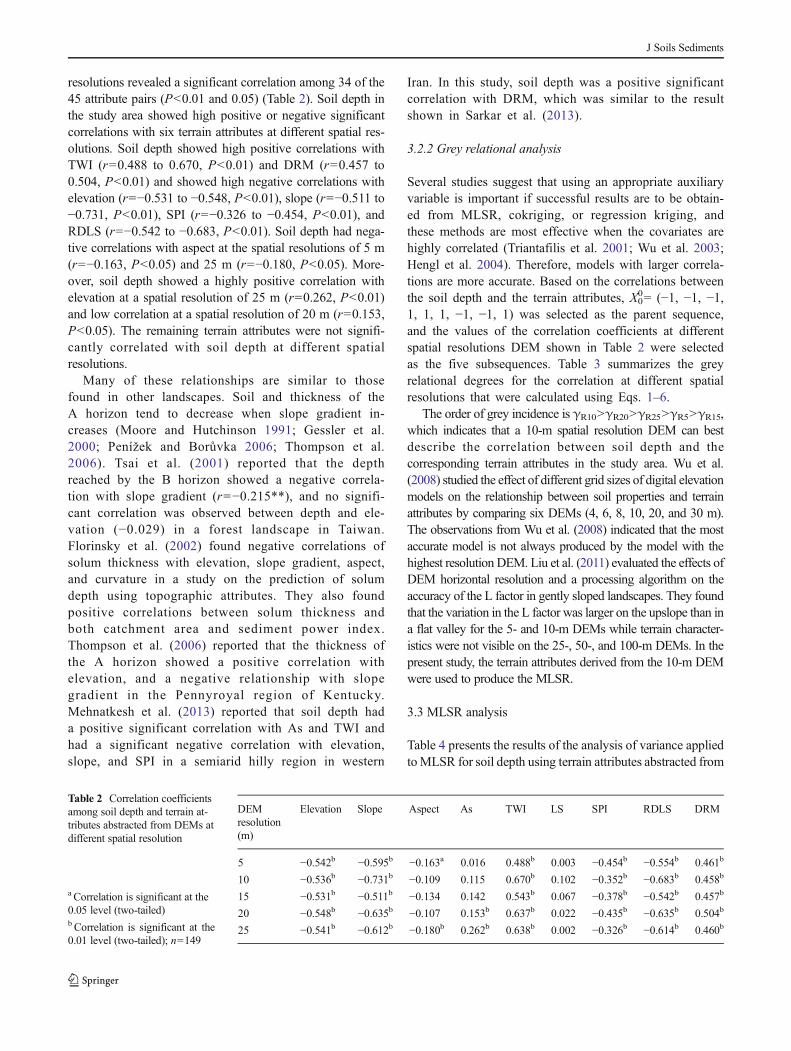
resolutions revealed a significant correlation among 34 of the45 attribute pairs (P<0.01 and 0.05) (Table 2). Soil depth inthe study area showed high positive or negative significantcorrelations with six terrain attributes at different spatial res-olutions. Soil depth showed high positive correlations withTWI (r=0.488 to 0.670, P<0.01) and DRM (r=0.457 to0.504, P<0.01) and showed high negative correlations withelevation (r=−0.531 to −0.548, P<0.01), slope (r=−0.511 to−0.731, P<0.01), SPI (r=−0.326 to −0.454, P<0.01), andRDLS (r=−0.542 to −0.683, P<0.01). Soil depth had nega-tive correlations with aspect at the spatial resolutions of 5 m(r=−0.163, P<0.05) and 25 m (r=−0.180, P<0.05). More-over, soil depth showed a highly positive correlation withelevation at a spatial resolution of 25 m (r=0.262, P<0.01)and low correlation at a spatial resolution of 20 m (r=0.153,P<0.05). The remaining terrain attributes were not signifi-cantly correlated with soil depth at different spatialresolutions.

Many of these relationships are similar to thosefound in other landscapes. Soil and thickness of theA horizon tend to decrease when slope gradient in-creases (Moore and Hutchinson 1991; Gessler et al.2000; Penížek and Borůvka 2006; Thompson et al.2006). Tsai et al. (2001) reported that the depthreached by the B horizon showed a negative correla-tion with slope gradient (r=−0.215**), and no signifi-cant correlation was observed between depth and ele-vation (−0.029) in a forest landscape in Taiwan.Florinsky et al. (2002) found negative correlations ofsolum thickness with elevation, slope gradient, aspect,and curvature in a study on the prediction of solumdepth using topographic attributes. They also foundpositive correlations between solum thickness andboth catchment area and sediment power index.Thompson et al. (2006) reported that the thickness ofthe A horizon showed a positive correlation withelevation, and a negative relationship with slopegradient in the Pennyroyal region of Kentucky.Mehnatkesh et al. (2013) reported that soil depth hada positive significant correlation with As and TWI andhad a significant negative correlation with elevation,slope, and SPI in a semiarid hilly region in western

Iran. In this study, soil depth was a positive significantcorrelation with DRM, which was similar to the resultshown in Sarkar et al. (2013).

3.2.2 Grey relational analysis

Several studies suggest that using an appropriate auxiliaryvariable is important if successful results are to be obtain-ed from MLSR, cokriging, or regression kriging, andthese methods are most effective when the covariates arehighly correlated (Triantafilis et al. 2001; Wu et al. 2003;Hengl et al. 2004). Therefore, models with larger correla-tions are more accurate. Based on the correlations betweenthe soil depth and the terrain attributes, X0

0= (−1, −1, −1,1, 1, 1, −1, −1, 1) was selected as the parent sequence,and the values of the correlation coefficients at differentspatial resolutions DEM shown in Table 2 were selectedas the five subsequences. Table 3 summarizes the greyrelational degrees for the correlation at different spatialresolutions that were calculated using Eqs. 1–6.

The order of grey incidence is γR10>γR20>γR25>γR5>γR15,which indicates that a 10-m spatial resolution DEM can bestdescribe the correlation between soil depth and thecorresponding terrain attributes in the study area. Wu et al.(2008) studied the effect of different grid sizes of digital elevationmodels on the relationship between soil properties and terrainattributes by comparing six DEMs (4, 6, 8, 10, 20, and 30 m).The observations from Wu et al. (2008) indicated that the mostaccurate model is not always produced by the model with thehighest resolution DEM. Liu et al. (2011) evaluated the effects ofDEM horizontal resolution and a processing algorithm on theaccuracy of the L factor in gently sloped landscapes. They foundthat the variation in the L factor was larger on the upslope than ina flat valley for the 5- and 10-m DEMs while terrain character-istics were not visible on the 25-, 50-, and 100-m DEMs. In thepresent study, the terrain attributes derived from the 10-m DEMwere used to produce the MLSR.

3.3 MLSR analysis

Table 4 presents the results of the analysis of variance appliedtoMLSR for soil depth using terrain attributes abstracted from

Table 2 Correlation coefficientsamong soil depth and terrain at-tributes abstracted from DEMs atdifferent spatial resolution

a Correlation is significant at the0.05 level (two-tailed)b Correlation is significant at the0.01 level (two-tailed); n=149

DEMresolution(m)

Elevation Slope Aspect As TWI LS SPI RDLS DRM

5 −0.542b −0.595b −0.163a 0.016 0.488b 0.003 −0.454b −0.554b 0.461b

10 −0.536b −0.731b −0.109 0.115 0.670b 0.102 −0.352b −0.683b 0.458b

15 −0.531b −0.511b −0.134 0.142 0.543b 0.067 −0.378b −0.542b 0.457b

20 −0.548b −0.635b −0.107 0.153b 0.637b 0.022 −0.435b −0.635b 0.504b

25 −0.541b −0.612b −0.180b 0.262b 0.638b 0.002 −0.326b −0.614b 0.460b

J Soils Sediments

10-m spatial resolution DEM, based on the regression results,slope, TWI, and elevation entered into the regression equationfor the model (F=70.64>3.93 at the 0.01 level (two-tailed)).Fitted equations and related parameters are as follows:

H ¼ 97:883−1:457� Slopeþ 2:688� TWI−0:073� ElevationR2 ¼ 0:614;P < 0:001� �

ð9Þ

The regression results showed that the correlations betweendepth and relevant auxiliary indices were highly significant,indicating that auxiliary variables contributed to the variabilityof depth to some extent. The adjusted coefficient of determi-nation (adj. R2) for the model can explain 61.4 % of thevariation of depth in the studied area. Gessler et al. (2000)indicated that models, which use only TWI could explain84 % of variation in soil depth in hillslopes of California.Thompson et al. (2006) indicated that multiple linear regres-sions models could explain 28 and 44 % of the variability ofA-horizon depth in central and east fields of the Pennyroyalregion of Kentucky mainly based on elevation, slope gradient,TWI, and the contribution of the upslope area. Usingtopographic attributes, Ziadat (2010) showed that multiplelinear regressions models predicted soil depth with a differ-ence of 50 cm for 77% of the field observations within a smallwatershed subdivision. A study in a semiarid hilly region inwestern Iran by Mehnatkesh et al. (2013) used regressionkriging to study the relationship between soil depth and terrainattributes; they reported that slope, TWI, and catchment areacan explain 84% of variation in soil depth. Sarkar et al. (2013)

used regression kriging to predict spatial variability of soildepth and reported that slope, aspect, general curvature, TWI,and land use were included in the MLR model they devel-oped, which explained 44% of spatial variability in soil depth.

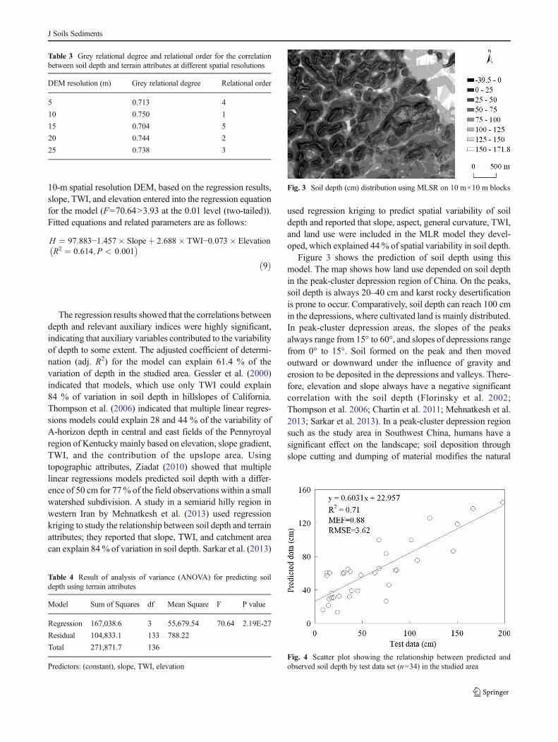
Figure 3 shows the prediction of soil depth using thismodel. The map shows how land use depended on soil depthin the peak-cluster depression region of China. On the peaks,soil depth is always 20–40 cm and karst rocky desertificationis prone to occur. Comparatively, soil depth can reach 100 cmin the depressions, where cultivated land is mainly distributed.In peak-cluster depression areas, the slopes of the peaksalways range from 15° to 60°, and slopes of depressions rangefrom 0° to 15°. Soil formed on the peak and then movedoutward or downward under the influence of gravity anderosion to be deposited in the depressions and valleys. There-fore, elevation and slope always have a negative significantcorrelation with the soil depth (Florinsky et al. 2002;Thompson et al. 2006; Chartin et al. 2011; Mehnatkesh et al.2013; Sarkar et al. 2013). In a peak-cluster depression regionsuch as the study area in Southwest China, humans have asignificant effect on the landscape; soil deposition throughslope cutting and dumping of material modifies the natural

Table 3 Grey relational degree and relational order for the correlationbetween soil depth and terrain attributes at different spatial resolutions

DEM resolution (m) Grey relational degree Relational order

5 0.713 4

10 0.750 1

15 0.704 5

20 0.744 2

25 0.738 3

Table 4 Result of analysis of variance (ANOVA) for predicting soildepth using terrain attributes

Model Sum of Squares df Mean Square F P value

Regression 167,038.6 3 55,679.54 70.64 2.19E-27

Residual 104,833.1 133 788.22

Total 271,871.7 136

Predictors: (constant), slope, TWI, elevation

Fig. 3 Soil depth (cm) distribution using MLSR on 10 m×10 m blocks

Fig. 4 Scatter plot showing the relationship between predicted andobserved soil depth by test data set (n=34) in the studied area

J Soils Sediments

gradient. People convert the steep-side slopes into flat landsfor the construction of home sites and other buildings and foragricultural practices. Anthropogenic disturbances are thecause of maximum soil thickness near the cultivated landand settlement sites, which was also observed by previousresearchers (Kuriakose et al. 2009; Chartin et al. 2011).

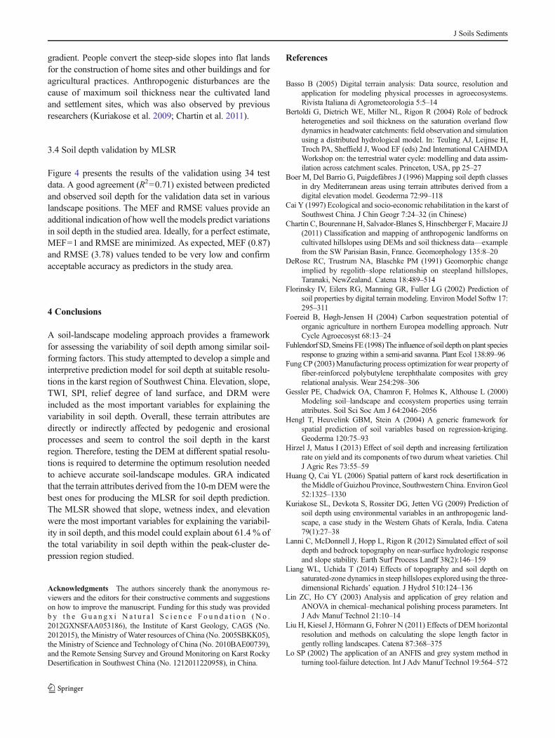
3.4 Soil depth validation by MLSR

Figure 4 presents the results of the validation using 34 testdata. A good agreement (R2=0.71) existed between predictedand observed soil depth for the validation data set in variouslandscape positions. The MEF and RMSE values provide anadditional indication of howwell the models predict variationsin soil depth in the studied area. Ideally, for a perfect estimate,MEF=1 and RMSE are minimized. As expected, MEF (0.87)and RMSE (3.78) values tended to be very low and confirmacceptable accuracy as predictors in the study area.

4 Conclusions

A soil-landscape modeling approach provides a frameworkfor assessing the variability of soil depth among similar soil-forming factors. This study attempted to develop a simple andinterpretive prediction model for soil depth at suitable resolu-tions in the karst region of Southwest China. Elevation, slope,TWI, SPI, relief degree of land surface, and DRM wereincluded as the most important variables for explaining thevariability in soil depth. Overall, these terrain attributes aredirectly or indirectly affected by pedogenic and erosionalprocesses and seem to control the soil depth in the karstregion. Therefore, testing the DEM at different spatial resolu-tions is required to determine the optimum resolution neededto achieve accurate soil-landscape modules. GRA indicatedthat the terrain attributes derived from the 10-mDEMwere thebest ones for producing the MLSR for soil depth prediction.The MLSR showed that slope, wetness index, and elevationwere the most important variables for explaining the variabil-ity in soil depth, and this model could explain about 61.4 % ofthe total variability in soil depth within the peak-cluster de-pression region studied.

Acknowledgments The authors sincerely thank the anonymous re-viewers and the editors for their constructive comments and suggestionson how to improve the manuscript. Funding for this study was providedb y t h e G u a n g x i N a t u r a l S c i e n c e F o u n d a t i o n ( N o .2012GXNSFAA053186), the Institute of Karst Geology, CAGS (No.2012015), the Ministry of Water resources of China (No. 2005SBKK05),the Ministry of Science and Technology of China (No. 2010BAE00739),and the Remote Sensing Survey and Ground Monitoring on Karst RockyDesertification in Southwest China (No. 1212011220958), in China.

References

Basso B (2005) Digital terrain analysis: Data source, resolution andapplication for modeling physical processes in agroecosystems.Rivista Italiana di Agrometeorologia 5:5–14

Bertoldi G, Dietrich WE, Miller NL, Rigon R (2004) Role of bedrockheterogeneties and soil thickness on the saturation overland flowdynamics in headwater catchments: field observation and simulationusing a distributed hydrological model. In: Teuling AJ, Leijnse H,Troch PA, Sheffield J, Wood EF (eds) 2nd International CAHMDAWorkshop on: the terrestrial water cycle: modelling and data assim-ilation across catchment scales. Princeton, USA, pp 25–27

Boer M, Del Barrio G, Puigdefábres J (1996) Mapping soil depth classesin dry Mediterranean areas using terrain attributes derived from adigital elevation model. Geoderma 72:99–118

Cai Y (1997) Ecological and socio-economic rehabilitation in the karst ofSouthwest China. J Chin Geogr 7:24–32 (in Chinese)

Chartin C, Bourennane H, Salvador-Blanes S, Hinschberger F,Macaire JJ(2011) Classification and mapping of anthropogenic landforms oncultivated hillslopes using DEMs and soil thickness data—examplefrom the SW Parisian Basin, France. Geomorphology 135:8–20

DeRose RC, Trustrum NA, Blaschke PM (1991) Geomorphic changeimplied by regolith–slope relationship on steepland hillslopes,Taranaki, NewZealand. Catena 18:489–514

Florinsky IV, Eilers RG, Manning GR, Fuller LG (2002) Prediction ofsoil properties by digital terrain modeling. EnvironModel Softw 17:295–311

Foereid B, Høgh-Jensen H (2004) Carbon sequestration potential oforganic agriculture in northern Europea modelling approach. NutrCycle Agroecosyst 68:13–24

Fuhlendorf SD, Smeins FE (1998) The influence of soil depth on plant speciesresponse to grazing within a semi-arid savanna. Plant Ecol 138:89–96

Fung CP (2003)Manufacturing process optimization for wear property offiber-reinforced polybutylene terephthalate composites with greyrelational analysis. Wear 254:298–306

Gessler PE, Chadwick OA, Chamron F, Holmes K, Althouse L (2000)Modeling soil–landscape and ecosystem properties using terrainattributes. Soil Sci Soc Am J 64:2046–2056

Hengl T, Heuvelink GBM, Stein A (2004) A generic framework forspatial prediction of soil variables based on regression-kriging.Geoderma 120:75–93

Hirzel J, Matus I (2013) Effect of soil depth and increasing fertilizationrate on yield and its components of two durum wheat varieties. ChilJ Agric Res 73:55–59

Huang Q, Cai YL (2006) Spatial pattern of karst rock desertification intheMiddle of Guizhou Province, Southwestern China. EnvironGeol52:1325–1330

Kuriakose SL, Devkota S, Rossiter DG, Jetten VG (2009) Prediction ofsoil depth using environmental variables in an anthropogenic land-scape, a case study in the Western Ghats of Kerala, India. Catena79(1):27–38

Lanni C, McDonnell J, Hopp L, Rigon R (2012) Simulated effect of soildepth and bedrock topography on near-surface hydrologic responseand slope stability. Earth Surf Process Landf 38(2):146–159

Liang WL, Uchida T (2014) Effects of topography and soil depth onsaturated-zone dynamics in steep hillslopes explored using the three-dimensional Richards’ equation. J Hydrol 510:124–136

Lin ZC, Ho CY (2003) Analysis and application of grey relation andANOVA in chemical–mechanical polishing process parameters. IntJ Adv Manuf Technol 21:10–14

Liu H, Kiesel J, Hörmann G, Fohrer N (2011) Effects of DEM horizontalresolution and methods on calculating the slope length factor ingently rolling landscapes. Catena 87:368–375

Lo SP (2002) The application of an ANFIS and grey system method inturning tool-failure detection. Int J Adv Manuf Technol 19:564–572

J Soils Sediments

Mehnatkesh A, Ayoubi S, Jalalian A, Sahrawat KL (2013) Relationshipbetween soil depth and terrain attributes in a semi arid hilly region inwestern Iran. J Mt Sci 10:163–172

Meyer MD, North MP, Gray AN, Zald HSJ (2007) Influence of soilthickness on stand characteristics in a Sierra Nevada mixed-coniferforest. Plant Soil 294:113–123

Minasny B, McBratney AB (1999) A rudimentary mechanisticmodel for soil production and landscape development.Geoderma 90:3–21

Moore ID, Hutchinson MF (1991) Spatial extension of hydrologic pro-cess modeling. Proc. Int. Hydrology and Water ResourcesSymposium. Institution of Engineers-Australia 91/22, pp 803–808

Odeh IOA, McBratney AB, Chittleborough DJ (1995) Further results onprediction of soil properties from terrain attributes: heterotopiccokriging and regression kriging. Geoderma 67:215–226

Palanikumar K, Latha B, Senthilkumar VS, Davim JP (2012) Analysis ondrilling of glass fiber–reinforced polymer (GFRP) composites usinggrey relational analysis. Mater Manuf Process 27:297–305

Pei T, Qin CZ, Zhu AX, Yang L, Luo M, Li BL, Zhou CH (2010)Mapping soil organic matter using the topographic wetness index:a comparative study based on different flow-direction algorithmsand kriging methods. Ecol Indic 10:610–619

Penížek V, Borůvka L (2006) Soil depth prediction supported by primaryterrain attributes: a comparison of methods. Plant Soil Environ 52:424–430

Sarkar S, Roy AK, Martha TR (2013) Soil depth estimation through soil-landscape modelling using regression kriging in a Himalayan ter-rain. Int J Geogr Inf Sci 27:2436–2454

Thompson JA, Pena-Yewtukhiw EM, Grove JH (2006) Soil–landscapemodeling across a physiographic region: topographic patterns andmodel transportability. Geoderma 133:57–70

Triantafilis J, Odeh IOA, McBratney AB (2001) Five geostatisticalmodels to predict soil salinity from electromagnetic induction dataacross irrigated cotton. Soil Sci Soc Am J 65:869–878

Tsai C, Chen Z, Duh C, Hong F (2001) Prediction of soil depth using asoil-landscape regression model: a case study on forest soils insouthern Taiwan. Proc Natl Sci Counc Repub China B Life Sci25:34–39

Uchida T, Tamura K, Mori N (2008) A simple method for producingprobabilistic shallow landslide hazard maps using soil thickness

dataset. European Geosciences Union General Assembly 2008:Geophysical Research Abstracts, vol. 10 (EGU2008-A-03941),Vienna, Austria. http://www.cosis.net/abstracts/EGU2008/03941/EGU2008-A-03941.pdf

Vereecken H, Jansen EJ, Hack-ten Broeke MJD, Swerts M, Engelke R,Fabrewitz S, Hansen S (1991) Comparison of simulation results offive nitrogen models using different data sets. Soil and GroundwaterResearch Report II: nitrate in soils pp 321–338

Wang J, Endreny TA, Hassett JM (2006) Power function decay ofhydraulic conductivity for a TOPMODEL-based infiltration routine.Hydrol Process 20:3825–3834

Wang GF, Zhao YG, Yang JL, Zhang GL, Zhao QG (2011) Predictionand mapping of soil depth at a watershed scale with fuzzy-c-meansclustering method. Soils 43:835–841

Wu JWA, Norvell DG, Hopkins DB, Smith MG, Ulmer RMW (2003)Improved prediction and mapping of soil copper by kriging withauxiliary data for cation-exchange capacity. Soil Sci Soc Am J 67:919–927

Wu W, Fan Y, Wang ZY, Liu HB (2008) Assessing effects of digitalelevation model resolutions on soil–landscape correlations in a hillyarea. Agric Ecosyst Environ 126:209–216

Xiong YJ, Qiu GY, Mo DK, Lin H, Sun H, Wang QX, Zhao SH, Yin J(2008) Rocky desertification and its causes in karst regions: a casestudy in Yongshun County, Hunan Province, China. Environ Geol57:1481–1488

Yang QY, Yang JS, Yao RJ, Huang B, Sun WX (2010) Comprehensiveevaluation of soil fertility by GIS and improved grey relation model.Trans CSAE 26:100–105 (in Chinese)

Yuan D (1993) The karst study of China. Geology Press, BeijingZhang M, Yuan H (1997) The PaūTa criterion and rejecting the abnormal

value. J Zhengzhou Univ Technol 18:84–88 (in Chinese)Zhang W, Chen HS, Wang KL (2006) Spatial variability of surface soil

water in typical depressions between hills in karst region in dryseason. Acta Pedol Sin 43:554–562

Zhang MY, Wang KL, Liu HY, Zhang CH (2011) Responses of spatial-temporal variation of karst ecosystem service values to landscapepattern in northwest of Guangxi, China Chin. Geogr Sci 21:446–453

Ziadat FM (2010) Prediction of soil depth from digital terrain data byintegrating statistical and visual approaches. Pedosphere 20:361–367

J Soils Sediments