regular symbolic analysis of dynamic networks of pushdown ... fileregular symbolic analysis of...

Regular Symbolic Analysis ofDynamic Networks of Pushdown Systems

Ahmed Bouajjani1, Markus Muller-Olm2, and Tayssir Touili1

1 LIAFA, University of Paris 7, 2 place Jussieu, 75251 Paris cedex 5, France2 Universitat Dortmund, FB 4, LS 5, Baroper Str. 301, 44221 Dortmund, Germany

Abstract. We introduce two abstract models for multithreaded programs basedon dynamic networks of pushdown systems. We address the problem of symbolicreachability analysis for these models. More precisely, weconsider the problemof computing effective representations of their reachability sets using finite-stateautomata. We show that, while forward reachability sets arenot regular in gen-eral, backward reachability sets starting from regular sets of configurations arealways regular. We provide algorithms for computing backward reachability setsusing word/tree automata, and show how these algorithms canbe applied for flowanalysis of multithreaded programs.

1 IntroductionMultithreaded programs are an important class of programs,in which parallelism isused routinely in practice. Parallel programming in general is known to be difficultand error prone, and multithreaded programs are no exception. Therefore, the designof methods and techniques for automatic analysis of such programs is an importantand a quite challenging issue. For that, we need to define formal models which areadequate for modelling multithreaded programs, and for which it is possible to constructautomatic analysis algorithms.

In recent related work, complete analysis algorithms for abstract classes of parallelprograms have been studied by several researchers. Mayr [14] establishes a number ofdecidability and undecidability results for process classes in the so-called PRS (processrewrite system) hierarchy. PRS are able to model sequentialas well as parallel phe-nomena. In fact, they can be seen as combinations of pushdownsystems and Petri nets(defined in a term rewriting setting using prefix and multisetrewrite rules). Followingthe automata-based approach for the symbolic verification of pushdown systems [2, 11],Lugiez and Schnoebelen [13] show how to use tree automata forreachability analysisof PA processes [1], a particularly well-known class in the PRS hierarchy. Their pa-per has inspired further work that applies tree automata techniques to analysis of moreexpressive models [6, 7, 3, 4, 21]. Another line of research generalizes fixpoint-basedtechniques as common in flow analysis to analysis of similar models of parallel pro-grams [20, 15, 16]. Both approaches can be used to solve bitvector problems, a certaintype of simple but important data-flow-analysis problems, for flow graph systems withparallel calls of procedures, or, equivalently, parbegin/parend-blocks interprocedurally[9, 10, 20]. While [9, 10] reduce the problem to reachabilityanalysis of PA-processes,[20] uses fixpoint-based techniques.

Unfortunately, these results donot cover interprocedural analysis of multithreadedprograms because commands that start new threads cannot adequately be modelled by

2 Ahmed Bouajjani, Markus Muller-Olm, and Tayssir Touili

parallel calls. In a multithreaded program such a command typically returns immedi-ately (see, e.g., the JAVA or POSIX thread API). Therefore the father of a new threadcan pursue its execution concurrently to its son and can eventerminate or return to itscaller while the son is still alive. In contrast, a parallel call returns only when and if allits component processes have terminated, which is a fundamentally different behavior.Indeed we show in Sect. 2 that in presence of procedures, multithreaded programs canhave trace languages different from that of any program withparallel calls.

The goal of this paper is to adapt the automata-based approach mentioned aboveto interprocedural (reachability) analysis of multithreaded programs. For this purposewe propose two models of multithreaded programs, show how toperform reachabilityanalysis for them with automata-theoretic constructions,and discuss their utility formodelling and analysing multithreaded and other classes ofparallel programs.

In Sect. 2 we introduceDynamic Pushdown Networks (DPNs)as a basic model ofmultithreaded programs. Intuitively, a DPN is a network of pushdown processes that runindependently in parallel. Each process can create new members of the network as a sideeffect of a pushdown transition. DPNs thus model a network ofthreads each of whichcan perform basic actions, call (recursively) procedures,andspawnnew processes. Weshow that while forward reachability of DPNs does not preserve regularity of configu-ration sets in general, it still preserves context-freeness (Sect. 4). Backward reachabilityin contrast preserves regularity and we show how to compute the backward reachabilityset of a regular set of configurations by means of a saturationalgorithm in polynomialtime (Sect. 4). We also show that DPN allow us to solve bitvector problems interproce-durally for multithreaded programs (Sect. 3), contrary to previously used models in theliterature such as PA processes (Sect. 2).

We extend DPNs toConstrained DPNs (CDPN)in Sect. 5, a model that combines(indeed even extends) the modelling power of both DPNs and PA(and even the so-called PAD [14]). The new idea is that enabledness of a transition for a process canbe made dependent on aconstraintwhich is a regular pattern among the sequence ofcontrol states of its sons. We require constraints to bestablein the sense that furtherevolution of the sons cannot invalidate a constraint. We show that otherwise we losethe property that backward reachability preserves regularity. Transition rules with sta-ble constraints increase the expressive power considerably over DPNs. In particularthey allow us to model, in addition to thread creation and procedure calls, also paral-lel calls and various types of join commands among other things. It also allows us toreturn information back from procedures called in parallelto their caller which cannotbe handled in PA and not even in PAD. Constrained DPNs inheritfrom DPNs that for-ward reachability does not preserve regularity. Therefore, we consider here backwardreachability only. We show that the set of configurations that can reach a given regularset of configurations of a CDPN can again be computed by a saturation algorithm. Asconfigurations of CDPNs are given by unbounded width trees rather than by words asin the DPN case—the tree structure captures the father-son relationship—we resort tohedge automata here [8]. The construction is nontrivial andits justification uses in asubtle manner the assumption about the stability of the constraints in the system defini-tion. While the overall complexity of this procedure is exponential—we indeed prove aPSPACE lower bound—it is exponential only in the number of different constraints used

Regular Symbolic Analysis of Dynamic Networks of Pushdown Systems 3

in the rules of the given CDPN, and just polynomial in the other problem parameters.Therefore, if the number of different constraints is bounded, we obtain a polynomial-time analysis algorithm. This in particular holds if we justmodel (in addition to spawnoperations), parallel calls, a fixed selection of join commands, or a combination of these.Due to lack of space, proofs are omitted. They can be found in [5].

2 Dynamic Pushdown NetworksA Dynamic Pushdown Network(DPN) is a tupleM = (Act,P,Γ,∆), whereAct is afinite set of visibleactions, P is a finite set ofcontrol states, Γ is a finite set ofstacksymbolsdisjoint fromP, and∆ is a finite set of transition rules of the following forms:

either (a)pγa→ p1w1, or (b) pγ

a→ p1w1 � p2w2, wherep, p1, p2 ∈ P, a∈ Act, γ ∈ Γ,

andw1,w2 ∈ Γ∗. A DPN can be seen as a collection of identical sequential processesrunning in parallel, each of them being able to (1) perform pushdown operations and to(2) create processes in the network. Synchronization is notallowed between processes.

A configuration of a DPNM (also calledM-configuration) is a word over the alpha-betΣ = P∪Γ starting with a symbol inP. An M-configuration can be seen as a sequenceof (sub)words inPΓ∗ each of them corresponding to the configuration of one of the pro-cesses running in parallel in the network. LetConfM be the set of allM-configurations.

For everya ∈ Act, we define a−→M to be the smallest relation inConfM ×ConfMs.t.∀u,v∈ ConfM, u a

−→M v iff (1) there is a rulepγa→ p1w1 in ∆ s.t.u = u1pγu2 and

v = u1p1w1u2, or (2) there is a rulepγa→ p1w1 � p2w2 in ∆ s.t. u = u1pγu2 andv =

u1p2w2p1w1u2. We writeu→M v if there existsa∈ Act s.t.u a−→M v.The semantics above says that rules of the form (a) correspond precisely to push-

down operations (manipulation of the top of the stack) whichcan be applied anywherein the configuration (i.e., by any of the processes in the network): if a process is atcontrol statep and hasγ as topmost stack symbol, then it can move to control statep1

and replaceγ by w1 at the top of its stack. Rules of the form (b) allow in additionthecreation of new processes: a process with control statep and topmost stack symbolγcan (1) move to statep1 and modify its stack by replacingγ with w1, and moreover, (2)create (to its left) a process which starts its execution at the initial configurationp2w2.

Given a configurationc, the set of immediate predecessors (resp. successors) ofc is preM(c) = {c′ ∈ C : c′→Mc} (resp.postM(c) = {c′ ∈ C : c→Mc′}). These no-tations can be generalized straightforwardly to sets of configurations. Letpre∗M (resp.post∗M) denote the reflexive-transitive closure ofpreM (resp.postM). We omit the sub-script M when it is understood from the context. Given∆′ ⊆ ∆, we usepre∆′ (resp.post∆′) to denote immediate predecessors (resp. successors) using a rule in∆′. Then,pre∗∆′ andpost∗∆′ denote the corresponding reflexive-transitive closures. Furthermore,

TracesM(c) = {w∈ Act∗ : ∃c′. cw→M c′} is the set of traces generated byc.

DPN vs. PA Processes:DPNs allow to model multithreaded programs where creationof threads is done using spawn commands (see Sect. 3). This isnot the case for otherformalisms used in the literature for modelling parallel programs like PA [1]:3

3 PA corresponds to processes definable by a set of rewrite rules of the formA→ t whereA isa process variable, andt is a term built from process variables, sequential composition, andasynchronous parallel composition.


Theorem 1. LetL =S

{an(bn′ ⊗(cmdm′

))

: n≥ n′ ≥ 0, m≥m′ ≥ 0}, where⊗ denotesthe shuffle (or interleaving) operator defined as usual. Then:

a) There is a DPN M and an M-configuration c such thatTracesM(c) = L.b) There is no PA system∆ and no process variable A such thatTraces∆(A) = L.

Hence, PA processes are inadequate for capturing the behavior of multithreaded pro-grams with spawn-like creation of threads. It also follows from the proof that trace setsof DPNs cannot be captured by the type of constraint systems used as semantic ref-erence point in the constraint-based approach [20, 15, 16].Therefore, the methods of[9, 10, 20, 16, 15] for interprocedural analysis of flow graphs with parallel calls do notcarry over immediately to multithreaded programs. These inadequacy results are ratherstrong because any interesting process equivalence would imply equality of traces.

3 Program Analysis Based on DPN

We show hereafter how DPNs can be used to model multithreadedprograms and howour results on symbolic reachability analysis can be used inflow analysis of these pro-grams. This is inspired by Esparza et. al. [9, 10].

Flow Graph Systems:As common in program analysis we assume that the programis given by a flow graph system. LetProc be a finite set of procedure names contain-ing Main . We assume that the program operates on a setX = {x1, . . . ,xk} of globalvariables. We consider the following types of basic statements: assignment statements,xi := e, wherexi ∈X ande is some expression; call of a single procedure,call(π), whereπ∈Proc; and spawn of a new thread,spawn(π), whereπ∈Proc. The intuitive meaningof assignment statements and calls is obvious. The spawn commandspawn(π) modelscreation of a new independent thread. Like the callcall(π), spawn(π) starts an instanceof procedureπ. In contrast to a call, however, the spawn command returns immedi-ately such that the newly created instance ofπ runs as a new thread concurrently to thestatements that are executed after the spawn. LetStmt be the set of basic statements.

The control flow of each procedureπ ∈ Proc is described by a control flow graphGπ = (Nπ,Eπ,eπ,xπ), whereNπ is a finite set of program points of procedureπ; Eπ ⊆Nπ ×Stmt×Nπ is a finite set of edges annotated by basic statements;eπ ∈ Nπ is theentry point ofπ; andxπ ∈ Nπ is the exit point ofπ. We assume that the sets of programpoints of different procedures are disjoint,Nπ∩Nπ′ = /0 if π,π′ ∈Proc, π 6= π′, and agreethatN =

S

π∈ProcNπ andE =S

π∈ProcEπ.

From Flow Graph Systems to DPN:From a given flow graph system as above weconstruct a DPNM = (Act,P,Γ,∆) that captures its operational semantics:

– The actions are given by the assignments that appear in the flow graph system;a special symbolτ is used to signify steps in which no assignment is executed:Act= {x := e | ∃u,v : (u,x := e,v) ∈ E}∪{τ};

– we have just one artificial control state #:P = {#};– we work with a stack of program points; the topmost stack symbol is the current

program point of the current procedure, the other stack symbols are the return pointsof its callers:Γ = N;


– the transition rules in∆ describe computation steps of the flow graph system:

1. for every assignment edge(u,x := e,v) ∈ E we put the rule #ux:=e→ #v to ∆;

2. for every call edge(u,call(π),v) ∈ E we put the rule #uτ→ #eπv to ∆;

3. for every spawn-edge(u,spawn(π),v) ∈ E we put the rule #uτ→ #v�#eπ to ∆,

4. for each procedureπ ∈ Proc, we put the rule #xπτ→ # to∆. This rule describes

the return from procedureπ.

Note that it is possible to extend the semantics above in order to handle local pro-cedure variables and return values from procedure calls. For that, we assume as usualthat data values are mapped into a finite abstract domain using standard techniques suchas predicate abstraction. Then, abstract values of local variables can be encoded in thestack alphabet and abstract return values can be encoded in the control states.

Solving Bitvector Problems:The operational semantics given above can be used forsolving bitvector problems. In order to ease comparison with [10] we discuss detectionof live (global) variables. Other bitvector problems can besolved in a similar fashion.Informally, a variablex ∈ X is live at a program pointu ∈ N if there is an executionfrom u in which x is used before it is over-written. We restrict attention toreachableconfigurations and use a similar definition and notation as Esparza and Podelski [10].Thus, we define: program variablex is live at a program pointu∈ N if there is a tran-sition sequence #eMain

σ1−−→c1σ2−−→c2

y:=e−−−→c3 such that: (1)u is activein configuration

c1, i.e., appears as the topmost stack symbol of one of the parallel pushdown processesin the network described byc1; (2) σ2 is a sequence of statements that do not modifyx(i.e., do not write tox); and (3)e is an expression in whichx is used.

We denote the set of configurationsc in which u is active byAtu, the set of assign-ments in the given program that modifyx by Modx ⊆ Act, and the set of assignmentsin the program in whichx is used byUsex ⊆ Act. Moreover, we write∆A for the set of

rules of∆ with an action in a subsetA⊆ Act: ∆A = {(pγa→ w) ∈ ∆ | a∈ A}. Using this

notation it is not hard to see thatx is live atu if and only if

#eMain ∈ pre∗(Atu∩pre∗∆Act\Modx(pre∆Usex

(ConfM)))

Then, our results concerning backward reachability analysis of DPN given in the nextsection (see Theorem 3 and Note 1) can be used to decide this property.

4 Reachability Analysis for DPN

We consider the problem of computing representations of thepost∗ andpre∗ images ofgiven sets of configurations. We are interested in the case that sets of configurations areeffectively given using automata-based representations.

Computing post∗ Images: We show first thatpost∗ does not preserve regularity in

general. Consider indeed the DPNM = ({a},{p},{γ1,γ2},{pγ1a→ pγ1γ1 � pγ2}). It is

easy to see thatpost∗M({pγ1}) = {(pγ2)npγn+1

1 : n≥ 0}, which is clearly nonregular.


Proposition 1. There is a DPN M, and a configuration c of M, such thatpost∗(c) isnot a regular set of configurations.

We prove, however, thatpost∗ preserves context-freeness:

Theorem 2. For every DPN M and any context-free set C of M-configurations, the setpost∗(C) is context-free and effectively constructible in polynomial time.

Computing pre∗ Images: We show now thatpre∗ preserves regularity. LetM be a DPNandA be an automaton recognizing a set ofM-configurations. We define a polynomial-time algorithm allowing to construct an automatonApre∗ s.t. L(Apre∗) = pre∗M(L(A)).For technical reasons, we require thatA is in a special form we define below.

M-Automata: Let M = (Act,P,Γ,∆) be a DPN. A finite automatonA = (S,Σ,δ,s0,F)is anM-automaton if the following conditions hold:

1. Σ = P∪Γ is the finite alphabet,2. the set of states is partitioned into two sets,S= Sc∪Ss, Sc∩Ss = /0,3. for everys∈ Sc and everyp∈ P, there is a (unique and distinguished) statesp ∈ Ss,4. there is a relationδ′ ⊆ Ss×Γ× (Ss\{sp : s∈ Sc, p∈ P}) ∪ Ss×{ε}×Sc such that

δ = δ′∪{(s, p,sp) : s∈ Sc, p∈ P},5. the initial states0 ∈ Sc, and6. F ⊆ S is the set of final states.

For σ ∈ Σ∪{ε} ands,s′ ∈ S, we writesσ→δ s′ in lieu of (s,σ,s′) ∈ δ. We extend

this notation in the obvious manner to sequences of symbols:(1)∀s∈ S. sε→δ s, and (2)

∀s,s′ ∈ S. ∀σ ∈ Σ∪{ε}. ∀w∈ Σ∗. s σw−−→δ s′ iff ∃s′′ ∈ S. s

σ→δ s′′ ands′′

w→δ s′.

Note that requirement (4) codes a number of conditions onδ: (1) eachs∈ Sc hassp as its uniquep-successor and has noΓ-transitions, (2)s is the only predecessor ofsp, (3) only ε-moves from states inSs lead to statess∈ Sc, (4) statess∈ Ss do nothave p-successors, for anyp ∈ P. So, every path in anM-automaton (starting fromthe initial state) is the concatenation of paths of the forms

p→δ sp

w−→δ tε→δ s′ where

s,s′ ∈ Sc, p∈ P, w∈ Γ∗, and all states in the pathspw−→δ t are inSs. Note that for every

finite automatonA over the alphabetP∪Γ such thatL(A) ⊆ ConfM, it is possible toconstruct anM-automaton recognizing the same language.

Constructing the AutomatonApre∗ : Let M be a DPN andA = (S,Σ,δ,s0,F) be anM-automaton. The construction ofApre∗ is in the same spirit as the ones for singlepushdown systems (see [2]). It consists in adding iteratively new transitions to the au-tomatonA according tosaturationrules (reflecting the backward application of thetransition rules in the system), while the set of states remains unchanged. Therefore,we defineApre∗ to be the finite-state automaton(S,Σ,δ′,s0,F), whereδ′ is the smallestrelation which containsδ (i.e.,δ ⊆ δ′) and satisfies the following conditions:

R1: If (pγa→ p1w1) ∈ ∆ ands

p1w1−−−→δ′ s′, for s,s′ ∈ S, then(sp,γ,s′) ∈ δ′.

R2: If (pγa→ p1w1 � p2w2) ∈ ∆ ands

p2w2p1w1−−−−−−→δ′ s′, for s,s′ ∈ S, then(sp,γ,s′) ∈ δ′.


The relationδ′ can be computed as the limit of an increasing sequence of relationsobtained by adding transitions toδ that are required by one of the implications above.This procedure terminates after a polynomial number of steps since only a polynomialnumber of transitions can potentially be added.

Let us explain intuitively the role of the saturation rule (R1). Consider a path in theautomaton of the forms p1w1−−−→s′. This means, by definition ofM-automata, thats is nec-essarily inSc and that we haves

p1−−→sp1

w1−−→s′. Then, the rule consists in adding to the

automaton the transitionspγ→ s′. Since by definition ofM-automata we haves

p→ sp, we

obtain a pathspγ

−−→s′ in the automaton. Therefore, if a configurationu1p1w1u2 is recog-nized by a runs0 u1−−→s

p1w1−−−→s′u2−−→sF , then its predecessoru1pγu2 is also recognized

due to the new transition by the runs0 u1−−→spγ

−−→s′u2−−→sF . The role of (R2) is similar.

Theorem 3. L(Apre∗) = pre∗M(L(A)

).

Note 1. For the sake of completeness, we mention that for every DPNM, and everyM-automatonA , the setspreM(A) andpostM(A) are regular and effectively constructible.The constructions are quite straightforward. ForpreM we take two copies ofA . The firstcopy provides the initial state and the second copy the final states. We then apply thesaturation rules to the first copy of the automaton, but let all new transitions lead fromstates of the first copy to states of the second copy. ThepostM construction is similar (itneeds adding a finite number of intermediary states).

5 Constrained DPN

We consider in this section an extension of the DPN model introduced in Section 2. Inaddition to the ability of performing spawn operation as previously, processes are nowallowed to observe the control states of their children (processes they have created inthe past). This is relevant in particular for handling return values and some kinds ofjoinstatements between parallel processes. To achieve that, wedefine a model where theapplication of a transition rule by some process is conditioned by a (regular language)constraint on the sequence of control states of its children. We need however to imposea stability condition (defined below) on the constraints in order to havea model whichcan be analysed by means of finite-state automata representations. We show later thatwe lose regularity of the reachability sets if we relax the stability condition.

Stable Regular Languages:Let Σ be a finite alphabet and letρ ⊆ Σ×Σ be a binaryrelation overΣ. Then, a set of symbolsS⊆ Σ is ρ-stable iff ∀s∈ S. ∀t ∈ Σ. (s,t) ∈ρ ⇒ t ∈ S. A ρ-stable regular language overΣ is a subset ofΣ∗ which is definable by aregular expression of the form:

e ::= S, aρ-stable set| e+e | e·e | e∗

We can prove straightforwardly by induction on the structure of regular expressions:

Lemma 1. Let φ ⊆ Σ∗ be aρ-stable regular language, let u,v∈ Σ∗, and let a∈ Σ suchthat uav∈ φ. Then, for every b∈ Σ, (a,b) ∈ ρ implies that ubv∈ φ.


Definition of the Models: A Constrained Dynamic Pushdown Network(CDPN) is atupleM = (Act,P,Γ,∆), whereAct is a finite set of visibleactions, P is a finite set ofcontrol states, Γ is a finite set ofstack symbolsdisjoint from P, and∆ is a finite set

of transition rules of the following forms: either (a)φ : pγa→ p1w1, or (b) φ : pγ

a→

p1w1 � p2w2, wherep, p1, p2 ∈ P, a ∈ Act, γ ∈ Γ, w1,w2 ∈ Γ∗, andφ is a ρ∆-stable

regular language overP, with ρ∆ = {(p, p′)∈P×P : there is a ruleψ : pδa→ p′u or ψ :

pδa→ p′u� p′′v in ∆}.A CDPN consists of a collection of identical sequential processes running in paral-

lel, each of them being modeled as a pushdown system which is able to (1) manipulateits own stack using pushdown rules of the form (a), (2) createa new process (whichbecomes its youngest son) using rules of the form (b), and (3)observe, under someconditions, the states of its children (processes it created in the past): each transitionrule is constrained by the fact that the sequence of control states of the children (givenin the decreasing order of their age) must belong to the specified languageφ.

Since we need to refer to the children of each process, a configuration of a CDPNcan be naturally seen as a tree where each vertex is annotatedwith the configurationof some sequential process (pushdown system), and where thestructure corresponds tothe relation father-son. Notice that such a tree may have an arbitrary width. We definehereafter a class of terms describing such configurations and we define a transitionrelation between such terms.

M-Terms: Let X = {x1, . . . ,xn} be a set of variables. We define the setT [X] of M-termsoverP∪Γ∪X inductively as follows:

– X ⊆ T [X],– If t ∈ T [X] andγ ∈ Γ, thenγ(t) ∈ T [X],– If t1, . . . ,tn ∈ T [X] andp∈ P, thenp(t1, . . . ,tn) ∈ T [X], for n≥ 0.

Note that in the last item of this definition,n can be 0 (i.e.,p is on a leaf). In thatcase, we writep() or simply p to represent the corresponding term.

Terms inT [ /0] are calledground terms, and will also be denoted byT . A termin T [X] is linear if each variable occurs at most once. Acontext Cis a linear term. Lett1, . . . ,tn benground terms. ThenC[t1, . . . ,tn] is the ground term obtained by substitutingin C the occurrence of the variablexi with the termti , for 1≤ i ≤ n.

A term inT [X] can be seen as a rooted labeled tree of arbitrary width, where(1) aninternal node is either of arity 1 (has one successor) if it islabeled with a stack symbolγ ∈ Γ, or it has an arbitrary arity if it is labeled with a statep ∈ P, and (2) where theleaves are labeled with either variablesx∈ X, or with statesp∈ P.

M-Configurations: We defineM-configurations to be the groundM-terms (terms inT [X] without variables). Givenn ground termst1, . . . ,tn, the termγm· · ·γ1p(t1, . . . ,tn)represents a configuration where (1) the common ancestor to all processes is at localcontrol statep and hasγ1 · · ·γm as stack content, whereγ1 is the topmost stack symbol,and (2) this process hasn children, theith of which is described, together with all ofits descendants, by the termti , for i = 1, . . . ,n. A ground term of the formγm· · ·γ1pcorresponds to the case of one single process without children.


Transition Relation: Given a CDPNM, we define a transition relation→M betweenM-configurations. We introduce first a notation. Given a configurationt of one of theforms γm· · ·γ1p(t1, . . . ,tn) or γm· · ·γ1p, we defineS(t) to be the control statep, i.e.,S(t) is the local control state of the topmost process represented in t. Then,→M is thesmallest relation betweenM-configurations such that:

– If (φ : pγa→ p1w1) ∈ ∆ andS(t1) · · ·S(tn) ∈ φ, then

C[γp(t1, . . . ,tn)

]→M C

[wR

1 p1(t1, . . . ,tn)]

– If (φ : pγa→ p1w1 � p2w2) ∈ ∆ andS(t1) · · ·S(tn) ∈ φ, then

C[γp(t1, . . . ,tn)

]→M C

[wR

1 p1(t1, . . . ,tn,wR2 p2)

]

wherewR denotes the reverse word (mirror image) ofw. The notions ofpost, pre, post∗,andpre∗ are defined as usual.

Modelling Power: Since CDPN generalize DPN, the modelling of programs withspawn operations given in Section 3 is still valid for CDPN. Moreover, stable con-straints as preconditions of transition rules increase tremendously the modelling powerof our formalism. We discuss some applications in this section.

Parallel Calls: In the data-flow analysis scenario, we can use constraints, e.g., in orderto accommodate parallel call commands as another basic primitive for creation of par-allelism in addition to spawn commands. A parallel call,pcall(π,π′) with π,π′ ∈ Procstarts an instance of procedureπ and an instance ofπ′ and runs them in parallel. Itterminates if and when both these instances terminate.

Assume that we extend the flow-graph model of Section 3 by allowing parallelcalls as another type of basic statement. In the CDPN model wecapture the operationalsemantics of an edge(u,pcall(π,π′),v) as follows: we start two new threads forπ andπ′

and ensure by a transition rule with an appropriate constraint that we can move tov onlyafter both these threads have terminated. For that, both threads indicate termination bymoving to a special new “terminated” control state♮ when they see a special new stacksymbol $ that we put at the bottom of their stack upon thread creation. Thus, we havethe following rules for modelling(u,pcall(π,π′),v):

P∗ : #uτ→ #γ1 �#eπ$ P∗ : #γ1

τ→ #γ2 �#eπ′$ P∗♮2 : #γ2

τ→ #v

whereγ1,γ2 are two auxiliary stack symbols chosen fresh for each parallel call. More-

over, the ruleP∗ : #$τ→ ♮ allows a thread to move to the state♮ once it has terminated.

Join Statements:Besides parallel calls we can also model different types of join-commands. We use the same technique as above for making termination visible to the

father of threads: we now use the rule #uτ→ #v� #ep$ to describe the behavior of a

spawn edge(u,spawn(p),v) ∈ E. Thus, we mark the bottom of the stack with the spe-

cial symbol $. We also use the ruleP∗ : #$τ→ ♮ from above to make termination visible


in the control state. This allows us to describe the operational semantics of differenttypes of join-command such as for instance (1)join∀: proceed if all threads directly cre-ated by the current thread have terminated, and (2)join∃k: proceed if at leastk amongthe threads directly created by the current thread have terminated.

The behavior of an edge(u, j,v) where j is one of the join commands from above

is modelled by the ruleφ : #uτ→ #v whereφ = ♮∗ for j = join∀, andφ = (P∗♮)kP∗ for

j =join∃k. Obviously, these constraints are stable.

Return Values:We can distinguish between different termination conditions by usingmore than one terminated control state and use regular patterns of such control statesin constraints in the father process. This allows us, for instance, to return informationback to the caller from procedures called in parallel. Therefore, the modelling power ofCDPNs exceeds that of PA and even that of PAD4 [14]: While in a PAD process (likein a DPN process) we can use control states to return information back to a caller ina normal procedure call, there is no such mechanism for parallel calls. The modellingpower for calls and parallel calls is thus more symmetric forCDPNs than for PAD.

Observing Execution Phases:Finally, as we allowstableconstraints, a creator of athread can react on situations in which the created thread has achieved some progressalready but is not necessarily terminated yet. As an example, let us assume that a processF (the father) creates a number of worker threads that sequentially go through a numberof phases, say phases 1, . . . ,n, before termination. For modelling the worker threads weuse new control states from a hierarchyP0 ⊃ P1 ⊃ . . . ⊃ Pn = /0 of control states suchthat a worker thread is in phasei if and only if its control state is inPi−1\Pi. This meansa worker thread has finished phasei if and only if its control state belongs toPi. Then,the setsPi are stable and can be used as building blocks for constraintsin transitions ofF . Hence, processF can react on situations like “all worker threads have finished phasei” by using the constraintP∗

i , “there is a worker thread that has finished phasei and allother worker threads have finished phasej” by the constraintP∗

j PiP∗j , etc.

6 Backward reachability analysis of CDPN

Symbolic Representations:We use hedge automata (unbounded width tree automata)[8] to represent infinite sets of CDPN configurations. LetM = (Act,P,Γ,∆) be a CDPN.An M-tree automatonis a tupleA = (Q,δ,F), whereQ is a set of states,F is the setof final states, andδ is a set of rules of either the form (1)γ(q) → q′, whereγ ∈ Γ, andq,q′ ∈ Q, or (2) p(L) → q, whereL is a regular language overQ, p∈ P, andq∈ Q.

In order to define the language recognized byA , we define amove relation→δbetween terms overP∪Γ∪Q: for every two termst andt ′, we havet →δ t ′ iff there exista contextC and a ruler ∈ δ such thatt = C[s], t ′ = C[s′], and (1) eitherr = γ(q) → q′,s= γ(q), ands′ = q′, or (2)r = p(L) → q, s= p(q1, . . . ,qn), q1 · · ·qn ∈ L, ands′ = q.

Let∗→δ denote the reflexive-transitive closure of→δ. A term t ∈ T is accepted by

q∈ Q if t∗→δ q. Let Lδ

q = {t ∈ T : t∗→δ q}. A term t is accepted byA if there exists a

stateq∈ F such thatt∗→δ q. Let L(A) be the set of all terms accepted byA .

4 PAD extends PA by allowing rewrite rules of the formA·B→ t


A straightforward adaptation of the proofs in [8] allows to show that:

Theorem 4. The class of M-tree automata is closed under boolean operations. More-over, the emptiness problem of M-tree automata is decidable.

Computing pre∗ Images: Let M = (Act,P,Γ,∆) be a CDPN and letA = (Q,δ,F)be anM-tree automaton. We present hereafter an algorithm that allows us to constructanM-tree automatonApre∗ recognizing thepre∗-image ofL(A). The construction pro-ceeds (similarly to Section 4) by adding new transitions to the original automatonAcorresponding to the backward application of transition rules. In order to deal with theconstraints in the transition rules, we need to extend the original automaton.

Propagating Control States:Remember that, by definition of CDPN terms, the con-figuration of each process is encoded bottom-up in the tree (reading first the controlstate, and then the stack contents starting from its topmostsymbol). Since constraintsin CDPN transition rules refer to control states of the children processes, and sincehedge automata can check only constraints on immediate successors in trees (whichcorrespond in our case to the bottom symbols in the stacks of the children processes),we need to propagate upward the informations about the control states through thestacks. Therefore, the first step of our construction consists in defining a new automa-ton AP = (QP,δP,FP) such thatL(AP) = L(A), and where states ofQ are labelled bycontrol statesp∈ P. This automaton is given by:QP = Q×P, FP = F ×P, andδP isthe smallest set of rules such that:

– if p(L) → s∈ δ, thenp(L′) → (s, p) ∈ δP, whereL′ is obtained by substituting inthe words ofL every occurrence of a states∈ Q by {(s, p) | p∈ P};

– if γ(s) → s′ ∈ δ, then for everyp∈ P, γ((s, p)

)→ (s′, p) ∈ δP.

Lemma 2. L(AP) = L(A), and for every t∈ T , t∗→δP (s, p) iff t

∗→δ s andS(t) = p.

Note 2. To avoid confusion, we use in the sequelp, p′, p1, p2, . . . to denote elements ofP, s,s′,s1,s2, . . . , to denote states ofA , andq,q′,q1,q2, . . . to denote states ofAP.

From Constraints over P to Constraints over QP: Given a constraintφ andn termst1, . . . ,tn such thatti

∗→δP

qi for 1≤ i ≤ n, we need also to be able to get the informationwhetherS(t1) · · ·S(tn) ∈ φ from the statesq1, . . . ,qn. For that, we associate with eachconstraintφ overP a constraint〈φ〉 overQP such thatS(t1) · · ·S(tn) ∈ φ if and only ifq1 · · ·qn ∈ 〈φ〉. The definition of〈φ〉 is straightforward by induction on the structure ofregular expressions for stable languages: (1)〈S〉= {(s, p) : s∈Q, p∈S}, (2)〈φ1 ·φ2〉=〈φ1〉 · 〈φ2〉, (3) 〈φ1 + φ2〉 = 〈φ1〉+ 〈φ2〉, and (4)〈φ∗〉 = 〈φ〉∗.

Closed Set of Constraints:During the construction of the automaton, new transitionrules of the formp(L′) → q are added whereL′ are languages which are built from lan-guagesL appearing in the rules of the original automatonA , and constraintsφ appearingin the transition rules of the CDPNM, using intersection and right-quotient operations.IntersectionsL∩〈φ〉 allow us to check that the guarding constraint for the application


of a transition rule is satisfied at the considered position in the tree. Right-quotientsLq−1 = {w : wq∈ L} allow us to get immediate predecessors by a spawn operation oftrees where the children of the spawning process are recognized by a sequence of statesin L, and the youngest son among these children (i.e., the one created by the spawnoperation and which is the right-most one in the list of children) is recognized by thestateq. Then, let us defineΛ to be the smallest family of languages overQP such that:

– If (p(L) → q) ∈ δP, thenL ∈ Λ.

– If L ∈ Λ, and(φ : pγa→ p1w1 � p2w2) ∈ ∆, thenL∩〈φ〉 ∈ Λ.

– If L ∈ Λ andq∈ QP, thenLq−1 ∈ Λ.

Lemma 3. The familyΛ is finite. Assuming that all languages and constraints appear-ing in rulesδP and∆ are given by backward-deterministic finite-state automataof sizeat most K, the number of elements ofΛ is in O(Kn+1) where n is the number of differentconstraints appearing in the rules of∆.

ConstructingApre∗ : We defineApre∗ to be theM-tree automaton(Q′,δ′,F ′) such that(1) Q′ = QP∪{qL

p : p∈ P, L ∈ Λ}, (2) F ′ = FP, and (3)δ′ is the smallest set of rulessuch thatδ′0 = δP∪{p(L) → qL

p : p∈ P, L ∈ Λ} ⊆ δ′ and:

R1: If (φ : pγa→ p′w) ∈ ∆, p′(L)→ q∈ δ′0, andwR(q)

∗→δ′ q′, then

(γ(qL∩〈φ〉

p )→ q′)∈ δ′.

R2: If (φ : pγa→ p′w1� p′′w2) ∈ ∆, p′(L) → q′′ ∈ δ′0, wR

1(q′′)∗→δ′ q′, andwR

2(p′′)∗→δ′ q,

then(γ(qLq−1∩〈φ〉

p ) → q′)∈ δ′.

Note that the statesqLp, for p ∈ P, andL ∈ Λ, are added to the automaton in order to

recognize precisely all the terms havingp at the root and such that the sequence ofchildren of the root is recognized by a sequence of states in the languageL. Note alsothat all the transitions added by the construction areΓ-transitions, and therefore they donot addP-transitions to the automaton.

The set of rulesδ′ can be computed iteratively as the limit of an increasing sequenceδ′0 ⊆ δ′1 · · · such thatδ′i+1 contains at most one transition more thanδ′i added by applyingeither(R1) or (R2). Note thatδ′ is necessarily finite since (by Lemma 3) the number oftriples(γ,qL

p,q), for γ ∈ Γ, p∈ P, L ∈ Λ, andq∈ Q′ is finite.

Lemma 4. For every q∈ QP, Lδ′q = pre∗(LδP

q ).

The lemma above says that the construction ensures that every state recognizes theset of all predecessors of its original language (i.e., in the automaton before saturation).Let us give some intuitive explanations about the role of thesaturation rules, and let usconsider the rule(R1) (since the role of(R2) is similar). Consider a termwRp′(t1, . . . ,tn)such thatti

∗→δ′ qi , for i ∈ {1, . . . ,n}. Assume thatp′(L) → q is a rule of the automaton.

This means that after recognizing each of the termsti and labelling their roots by thestatesqi, the automaton can label the termp′(t1, . . . ,tn) by q if the sequenceq1 · · ·qn isin L. Assume furthermore thatwR(q)

∗→δ′ q′. This means that the automaton can pro-

ceed by reading upward the wordw and label the termwRp′(t1, . . . ,tn) by q′. Therefore,


if (φ : pγa→ p′w) is a transition rule of the system, and if the sequence of control states

S(t1) · · ·S(tn) is in φ, then we must add the termγp(t1, . . . ,tn) (which is the immedi-ate predecessor ofwRp′(t1, . . . ,tn) by the transition rule) to the language ofq′ (to saythat this term is a predecessor of some term which was recognized byq′ in the originalautomaton). This is achieved by applying the saturation rule which adds to the automa-

ton the transition(γ(qL∩〈φ〉p ) → q′). The justification of this is in fact subtle. First, if

S(t1) · · ·S(tn) ∈ φ, we must haveq1 · · ·qn ∈ 〈φ〉. Since states recognize predecessors ofterms in their original language, each stateqi is a pair(si , p′i) such thatp′i = S(t ′i ) forsomet ′i such thatti ∈ pre∗(t ′i ). Now, here is the point where the stability property ofφ plays a crucial role: it ensures that backward transitions cannot make a term satisfynew constraints (or equivalently, that forward transitions cannot falsify a constraint).Therefore, sinceS(t1) · · ·S(tn)∈ φ, we must have alsoS(t ′1) · · ·S(t ′n)∈ φ, which impliesthatq1 · · ·qn ∈ 〈φ〉. On the other hand, assume thatS(t1) · · ·S(tn) 6∈ φ butq1 · · ·qn ∈ 〈φ〉becauseS(t ′1) · · ·S(t ′n) ∈ φ. We can show thatγp(t1, . . . ,tn) is actually in thepre∗ imageof the original language. Indeed, it is possible in this caseto start by rewriting each term

ti to its successort ′i , which makes the transition rule(φ : pγa→ p′w) applicable.

Theorem 5. For every CDPN M, and for every M-tree automatonA , we can constructan M-tree automatonApre∗ such that L(Apre∗) = pre∗

(L(A)

).

Note 3. It is easy to show that, given anM-tree automatonA , the setpreM(A) (and infact also the setpostM(A)) is an effectivelyM-tree automata definable set.

Then, based on the modelling described in Sections 3 and 5, wecan apply Theo-rems 5 and 4 to check reachability properties and solve flow analysis problems (such asbitvector problems) for multithreaded programs.

Complexity Issues:By Lemma 3, we know that the size of the automatonApre∗ is atmost exponential in the number of constraints appearing in the given CDPN. In fact,we can prove the following PSPACE lower bound by a reduction of the satisfiabilityproblem for quantified Boolean formulas (QBF).

Theorem 6. It is at least PSPACE-hard to decide for a given CDPN M, a regular setof M-configurations R and an M-configuration c, whether c∈ pre∗(R) or not.

Despite the hardness result above, in many interesting cases, we only need afixednum-ber of constraints, which leads to polynomial analysis algorithms. For instance, this isthe case when only trivial constraints (i.e., of the formP∗) are used, which correspondsto the case of DPN models. Also, to model parallel calls only one additional constraintis needed, namelyP∗♮2, as we have seen in Section 5. Similarly, we only need oneadditional constraint for each type of join statement such as join∀ or join∃k. Note thatthe automata for these constraints can easily be defined by backward deterministic au-tomata of very small sizes. Also for typical properties suchas bitvector problems (seeSection 3), the initial automaton is always the one recognizing the set of all configu-rations. Therefore, for an important fragment of CDPN whichsubsumes (in modellingpower) existing formalisms such as PA and PAD, and allows us in addition to modelspawn operations, our construction leads to a polynomial analysis algorithm.


However, when return values from parallel processes are taken into account, ourconstruction becomes exponential in the number of used abstract data values. This priceis unavoidable since dealing with an unfixed domain of returnvalues is precisely thefeature which makes our model complex (see the proof of Theorem 6). Such complexitydoes not appear for weaker models such as PA or PAD (which havepolynomial analysisalgorithms [13, 10, 6]) since they cannot handle return values from parallel processes.

Relaxing Stability:We end this section by mentioning the fact that relaxing the stabilitycondition on the constraints appearing in the transition rules of CDPN leads to a modelfor whichpre∗ images are not regular in general.

Theorem 7. There exists a CDPN M with nonstable constraints, and a regular set T ofM-configurations such thatpre∗M(T) is not definable by an M-tree automaton.

Actually, we can defineM s.t. all its transition rules are of the formφ : pγ → p′γ (i.e.,without stack manipulation and dynamic creation of processes), and whereφ is of thesimple formpP∗, for p∈ P. This shows that it is hard to relax the stability condition inthe definition of CDPN without losing the property thatpre∗ preserves regularity.

7 Conclusion

We have defined new formalisms (DPN and CDPN), based on word/term rewrite sys-tems, allowing to model adequately spawn-like commands in multithreaded programs.We have shown that (1) they are more suitable for modelling these commands thanpreviously proposed formalisms (such as PA and PAD), and that (2) they subsume infact in modelling power these models (concerning CDPN), andallow to handle featuresthese models cannot handle such as return values from parallel processes, various joincommands, etc.

We have defined automata-based techniques for computing backward reachabilitysets of our models. In the case of the basic model of DPN, word automata can be usedfor this purpose and the construction is simple. In the case of CDPN where constraintson the children are used, the problem of reachability analysis becomes much moredelicate. The condition of stability we impose in CDPN on theconstraints (guards)appearing in the transition rules seems to be necessary in order to have regular backwardreachability sets. Concerning complexity, our construction is exponential in the numberof different constraints used in the model, but significant classes of parallel programscan be modelled using a fixed number of constraints (often representable using smallautomata), and therefore they can be analysed in polynomialtime.

Future work includes the extension of our models and our approach to handle syn-chronisation between parallel processes. Of course, the reachability analysis becomesundecidable in general, but reasonable classes of programswith particular synchroni-sation policies can be considered (see e.g., [18]), and generic frameworks for definingabstractions (and refining them) can be developed based on our models and our tech-niques, e.g., following the approaches of [3, 4, 15]. We think also that our techniquescould be used to handle models which extend those consideredin this paper by allow-ing a bounded number of context switches, in the spirit of theapproach of [19].


References

1. J. Baeten and W. Weijland. Process Algebra. InCambridge Tracts in Theoretical ComputerScience, volume 18, 1990.

2. A. Bouajjani, J. Esparza, and O. Maler. Reachability Analysis of Pushdown Automata: Ap-plication to Model Checking. InCONCUR’97. LNCS 1243, 1997.

3. A. Bouajjani, J. Esparza, and T. Touili. A Generic Approach to the Static Analysis of Con-current Programs with Procedures. InPOPL’03. ACM, 2003.

4. A. Bouajjani, J. Esparza, and T. Touili. Reachability Analysis of Synchronised PA systems.In INFINITY’04. to appear in ENTCS, 2004.

5. A. Bouajjani, M. Muller-Olm, and T. Touili. Regular Symbolic Analysis of Dynamic Net-works of Pushdown Processes. Technical report, LIAFA lab No2005-05, and University ofDortmund No 798, June 2005.

6. A. Bouajjani and T. Touili. Reachability Analysis of Process Rewrite Systems. InFSTTCS’03. LNCS 2914, 2003.

7. A. Bouajjani and T. Touili. On Computing Reachability Sets of Process Rewrite Systems. InRTA’05. LNCS, 2005.

8. A. Bruggemann-Klein, M. Murata, and D. Wood. Regular Treeand Regular Hedge Lan-guages over Unranked Alphabets. Research report, 2001.

9. J. Esparza and J. Knoop. An Automata-Theoretic Approach to Interprocedural Data-FlowAnalysis. InFoSSaCS’99, volume 1578 ofLNCS, 1999.

10. J. Esparza and A. Podelski. Efficient Algorithms for pre∗ and post∗ on Interprocedural Par-allel Flow Graphs. InPOPL’00. ACM, 2000.

11. A. Finkel, B. Willems, and P. Wolper. A Direct Symbolic Approach to Model CheckingPushdown Systems. InInfinity’97, ENTCS 9. Elsevier Sci. Pub., 1997.

12. J. E. Hopcroft and J. D. Ullman.Introduction to Automata Theory, Languages and Compu-tation. Addison-Wesley, 1979.

13. D. Lugiez and P. Schnoebelen. The Regular Viewpoint on PA-Processes.Theoretical Com-puter Science, 274(1-2):89–115, 2002.

14. R. Mayr. Decidability and Complexity of Model Checking Problems for Infinite-State Sys-tems. Phd. thesis, Technical University Munich, 1998.

15. M. Muller-Olm. Variations on Constants. Habilitationsschrift, Fachbereich Informatik, Uni-versitat Dortmund, 2002.

16. M. Muller-Olm. Precise Interprocedural Dependence Analysis of Parallel Programs.Theo-retical Computer Science, 311:325–388, 2004.

17. C. H. Papadimitriou.Computational Complexity. Addison-Wesley, 1994.18. S. Qadeer, S. Rajamani, and J. Rehof. Procedure Summaries for Model Checking Multi-

threaded Software. InPOPL’04, 2004.19. S. Qadeer and J. Rehof. Context-Bounded Model-Checkingof Concurrent Software. In

TACAS’05. LNCS 3440, 2005.20. H. Seidl and B. Steffen. Constraint-based Interprocedural Analysis of Parallel Programs. In

ESOP’2000. LNCS 1782, 2000.21. T. Touili. Dealing with Communication for Dynamic Multithreaded Recursive Programs. In

1st VISSAS workshop, March 2005. Invited Paper.


AppendixWithout further ado, we present here the proofs that were omitted due to lack of space.We assume the notation and definitions from the main body of the paper.

A Proof of Theorem 1,a

Theorem 1,a.There is a DPNM with a single control state, and anM-configurationcsuch thatTracesM(c) = L.

Proof: Consider the DPNM = (Act,P,Γ,∆) with

– Act= {a,b,c,d},– P = {p},– Γ = {A,B,C,D},

– ∆ = {pAa→ pAB, pA

a→ pB� pC, pB

b→ p, pC

c→ pCD, pC

c→ pD, pD

d→ p}.

Ignoring the spawn in the second rule, the first three rules describe a push down au-tomaton that from control statep and initial stack contentsA accepts the languageanbn,n > 0 upon empty stack. This push down automaton generates the tracesanbn′ withn≥ n′ ≥ 0. When moving from the mode in which it generatesa’s to the mode in whichit generatesb’s, i.e., when executing the second rule, it spawns a second push down au-tomaton that acceptscmdm, m> 0, upon empty stack and which has the tracescmdm′

form≥ m′ ≥ 0. These traces are arbitrarily interleaved with the sequence ofb’s generatedby the first push down automaton. Hence we have:TracesM(pA) = L. 2

B Proof of Theorem 1,b

Theorem 1,b.There is no PA system∆ and no variableA such thatTraces∆(A) = L.

In order to prove Theorem 1,b, we need to introduce some definitions first. Letr = a1 · · ·al ∈ Act∗ be a trace andI = {i1, . . . , ik} be a subset of positions inr such that1 ≤ i1 < i2 < · · · < ik ≤ l . Then,r|I denotes the traceai1 · · ·aik. We write |r| for thelength ofr.

Given two tracesr, r ′ ∈ Act∗, the shuffle languager ⊗ r ′ ⊆ Act∗ is given by:r ⊗ r ′ ={s∈Act∗ : ∃I ⊆{1, . . . , |s|}. s|I = r ands|({1, . . . , |s|}\ I) = r ′}. This definition is liftedto sets of traces in the obvious way.

A shuffle-constraint system Sover a finite set of variablesY—the variables inYrange over subsets ofAct∗—is a finite set of subset constraints of the formA⊇ ti , whereA is a variable fromY andti is a term formed with the operators “·” (concatenation)and “⊗” (shuffle) from the variables inY and the languages{a}, for a∈ Act, and{ε}.Both concatenation and shuffle operations distribute over arbitrary unions and are thusmonotonic and even continuous. Thus, each shuffle-constraint systemS has a small-est solutionµS: Y → 2Act∗ by the Knaster-Tarski fixpoint theorem. It can be seen thatshuffle-constraint systems generalize context-free grammars to a parallel setting. It can


be shown [20, 16, 15, 4] that these systems generate precisely the set of traces that canbe generated by PA processes: processes definable by a set of rewrite rules of the formA → t whereA is a process variable, andt is a term built from process variables, se-quential composition, and asynchronous parallel composition [1].

Then, part b of Theorem 1 is an immediate consequence of the following result:

Theorem 8. There is no shuffle-constraint system S over some set of variables Y suchthat (µS)(A) = L for some A∈Y.

Proof: Assume there is a shuffle-constraint systemSoverY such that(µS)(A) = L forsomeA∈Y.

Our goal is to exhibit a pumping argument in order to deduce a contradiction. Wefirst argue that for each word inz∈ (µS)(A) we can find ajustifying treesimilar to aderivation tree for words of a context-free language. In a derivation tree in a context-freelanguage, we just need to keep the non-terminals and the terminals, because only theconcatenation operator is applied. Here we need to distinguish applications of concate-nation from applications of shuffle. Therefore, we put theseoperators at inner nodesof the tree. We also keep the variables/non-terminals in order to get a handle for thepumping argument. Thus, justifying trees are obtained in the following way:

1. we start from a tree that consists just of a root annotatedA.2. then we iterate the following step until all leafs of the tree are annotated by an

action: we replace a nonterminalB at a leaf by a subtree with rootB that has asingle successor that is the root of a tree corresponding tot for some constraintB⊇ t of S.

We can assign a set of action sequencesL(T) to each justifying treeT in a natural in-ductive way: a leaf annotated witha ∈ Act is assigned the language{a}; to an innernode annotated with a concatenation or shuffle operator, we assign the language ob-tained as the concatenation or shuffle, respectively of the languages associated with thesubtrees; finally for an inner node anotated with a variable,we associate the language ofits subtree. Clearly, the language of each justifying tree is contained in(µS)(A) becauseit is the language of a finite unfolding of the constraints. Conversely, we can find foreach wordz∈ (µS)(A) a justifying treeT: this follows from the well-known fixpointtheorem of Kleene. All the operators used in a shuffle-constraint system are continuous.Therefore, by Kleene’s fixpoint theorem, for each action sequencew ∈ (µS)(A) thereis k ≥ 0 such thatz is contained in thek-fold unfolding of the constraint system. Thisk-fold unfolding gives rise to a justifying tree.

Due to the presence of shuffle operators in the tree we do not necessarily findz atthe frontier of a justifying tree forz but the frontier is always some reordering ofz.Note, however, that the word at the frontier of a justifying treeT always belongs toL(T) because the concatenation of two languages is contained in their shuffle.

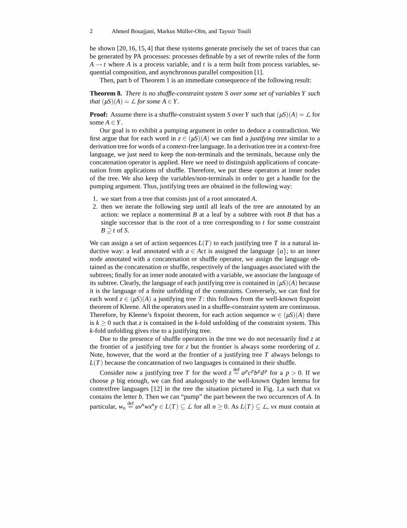
Consider now a justifying treeT for the wordzdef= apcpbpdp for a p > 0. If we

choosep big enough, we can find analogously to the well-known Ogden lemma forcontextfree languages [12] in the tree the situation pictured in Fig. 1,a such thatvxcontains the letterb. Then we can “pump” the part beween the two occurences ofA. In

particular,wndef= uvnwxny ∈ L(T) ⊆ L for all n≥ 0. As L(T) ⊆ L, vx must contain at


b

b

A

A

A

A

vu

v w x

x yyxwvu

a) b)

Fig. 1. Repetition of variableA on the path to ab symbol.

least as manya’s thanb’s. By looking at the leftmostv in the wordw2 = uvvwxxy∈ L

we infer thatv cannot contain any of the lettersb, c, or d becauseL contains no wordsin which one of the lettersb, c or d is left of ana (anda is found in eitherv or x).

If x would contain ad, vxmust contain ac for counting reasons aswn ∈ L for all n.As v cannot contain ac (see above), such ac must appear inx. But then inw2 ac wouldoccur to the right of ad which is not allowed byL. Hencex does not contain ad.

Of course there is also nod in u because otherwise we would have ad left of anaalready inw1 which is forbidden byL.

There can also be nod in w: assume there would be ad in w. In w all thed symbolsappear right of allb symbols. Therefore, there must be a shuffle operator betweenthetwo occurence ofA in order to generatew with T. But then we can generate with thetree forw2 also a word in which ana appear right of ab in contradiction toL (seeFig. 1,b).

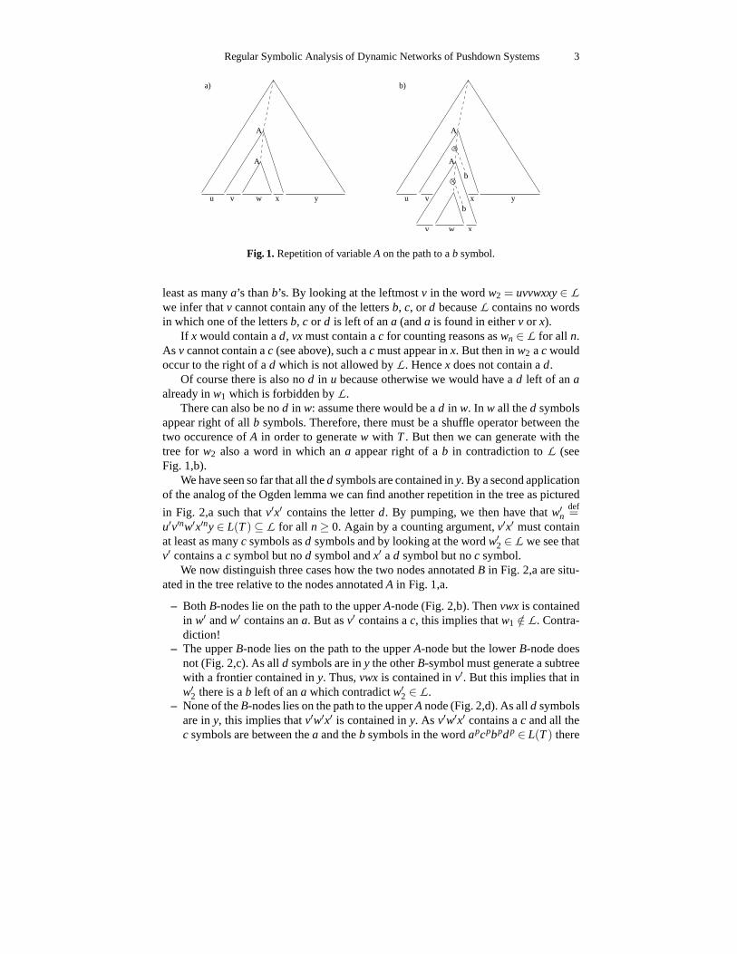
We have seen so far that all thed symbols are contained iny. By a second applicationof the analog of the Ogden lemma we can find another repetitionin the tree as pictured

in Fig. 2,a such thatv′x′ contains the letterd. By pumping, we then have thatw′n

def=

u′v′nw′x′ny∈ L(T) ⊆ L for all n≥ 0. Again by a counting argument,v′x′ must containat least as manyc symbols asd symbols and by looking at the wordw′

2 ∈ L we see thatv′ contains ac symbol but nod symbol andx′ a d symbol but noc symbol.

We now distinguish three cases how the two nodes annotatedB in Fig. 2,a are situ-ated in the tree relative to the nodes annotatedA in Fig. 1,a.

– BothB-nodes lie on the path to the upperA-node (Fig. 2,b). Thenvwx is containedin w′ andw′ contains ana. But asv′ contains ac, this implies thatw1 /∈ L. Contra-diction!

– The upperB-node lies on the path to the upperA-node but the lowerB-node doesnot (Fig. 2,c). As alld symbols are iny the otherB-symbol must generate a subtreewith a frontier contained iny. Thus,vwx is contained inv′. But this implies that inw′

2 there is ab left of ana which contradictw′2 ∈ L.

– None of theB-nodes lies on the path to the upperA node (Fig. 2,d). As alld symbolsare iny, this implies thatv′w′x′ is contained iny. As v′w′x′ contains ac and all thec symbols are between thea and theb symbols in the wordapcpbpdp ∈ L(T) there


d)

A

A

B

B

u’ v’ w’ x’ y’

a)

B

B

u’ v’ w’ x’ y’

c)

A

A

B

B

u’ v’ w’ x’ y’v w x

b)

A

A

B

B

x’ y’w’u’ v’wv x

Fig. 2. Repetition of variableB on the path to ad symbol.

must be a shuffle operator at the join point of the two pathes from the upperA andupperB to the root of the tree. But thenL(T) also contains a word in which ac isleft of ana which contradictsL(T) ⊆ L.

2

C Proof of Theorem 2

Theorem 2.For every DPNM and any context-free setC of M-configurations, the setpost∗(C) is context-free and effectively constructible in polynomial time.

Proof: Let M = (Act,P,Γ,∆) be a DPN andC be a regular set of configurations. First,we show that, for every pair(p,γ) ∈ P×Γ, the setpost∗({pγ}) is effectively definableby means of a context-free grammar.

We define a set of nonterminal symbolVN as the smallest set such that:

– If p, p′ ∈ P andγ ∈ Γ, then〈p,γ〉 ∈VN and〈p,γ, p′〉 ∈VN,– If pγ

a→ p1w1[�p2w2] ∈ ∆ and p′ ∈ P, then〈p1,w1〉 ∈ VN, [〈p2,w2〉 ∈ VN,] and

∀p′ ∈ P, 〈p1,w1, p′〉 ∈VN.

The set of productions is the smallest set such that:

– If p∈ P andγ ∈ Γ, then we have the production

〈p,γ〉 → pγ


– For every rule

pγa→ p1α1 · · ·αn[�p2β1 · · ·βm]

we have the productions:

〈p,γ〉 → [〈p2,β1 · · ·βm〉]〈p1,α1 · · ·αn〉

〈p,γ, p′〉 → [〈p2,β1 · · ·βm〉]〈p1,α1 · · ·αn, p′〉 wherep′ ∈ P

– ∀p, p′ ∈ P, ∀γ1 · · ·γn ∈ Γ, we have the productions

〈p,ε〉 → p

〈p,γ1 · · ·γn〉 → 〈p,γ1〉γ2 · · ·γn wheren≥ 1

〈p,γ1 · · ·γn〉 → 〈p,γ1,q1〉〈q1,γ2,q2〉 · · · 〈qi−1,γi ,qi〉〈qi ,γi+1〉γi+2 · · ·γn

wheren≥ 2, i ∈ {1, . . . ,n−1}, andq1, . . . ,qi ∈ P

and the productions

〈p,ε, p〉 → ε〈p,γ1 · · ·γn, p′〉 → 〈p,γ1,q1〉〈q1,γ2,q2〉 · · · 〈qn−1,γn, p′〉

wheren≥ 1, andq1, . . . ,qn−1 ∈ P.

Then, it can be checked that teh following holds.

Lemma 5. ∀p, p′ ∈ P,∀w∈ Γ∗, we have

– L(〈p,w〉) = post∗({pw}) .– L(〈p,w, p′〉) =

(post∗({pw})∩Σ∗p′

)(p′)−1 . ⊓⊔

Now, we define a transducerτ which associates with every configurationc∈ Σ∗ the setpost∗(c). The transducerτ has a finite set of states and transitions labeled by pairs ofthe form(w,L) wherew is an input word, andL is a context-free set of output words.The set of states ofτ is {q0,qcopy}∪{p : p∈ P}, the stateq0 is the unique initial andaccepting state, and the set of transitions is as follows:

q0(pγ,〈p,γ〉)

−−−−−−→ qcopy

q0(pγ,〈p,γ,p′〉)

−−−−−−−→ p′

p(γ,〈p,γ〉)−−−−−→ qcopy

p(γ,〈p,γ,p′〉)−−−−−−−→ p′

qcopy(p,p)−−−→ qcopy

qcopy(γ,γ)−−−→ qcopy

qcopy(ε,ε)

−−−→ q0

The result follows immediatly from the fact that context-free languages are closedunder context-free transductions, i.e., given a context-free set of configurationsC (ef-fectively defined by, e.g., a context-free grammar), the setτ(C) is context-free and ef-fectively constructible. 2


D Proof of Theorem 3

Let M be a DPN,A be anM-automaton andApre∗ be the automaton obtained by thesaturation procedure described in Section 4.

Theorem 3.L(Apre∗) = pre∗M(L(A)

).

Let us first consider the easier inclusion.

Lemma 6. pre∗M(L(A)) ⊆ L(Apre∗).

Proof: Clearly, pre∗M(L(A)) =S

k≥0prekM(L(A)). We show by induction onk that

prekM(L(A)) ⊆ L(Apre∗) for all k≥ 0.The induction base,k = 0, is obvious as the saturation procedure just adds transi-

tions such thatpre0(L(A)) = L(A) ⊆ L(Apre∗).Now, supposek ≥ 0 is given and assume thatprek

M(L(A)) ⊆ L(Apre∗) (inductionhypothesis). Consider an arbitrary configurationc∈ prek+1

M (L(A)). Then there is a con-figurationd ∈ prek

M(L(A)) and an actiona ∈ Act such thatca→ d, i.e., there is a rule

pγa→ p1w1 or pγ

a→ p1w1� p2w2 in ∆ as well asu,v∈ (P∪Γ)∗ such thatc= upγv and

d = urv for r = p1w1 or r = p2w2p1w1, respectively. By the induction hypothesis,d isaccepted byApre∗ , i.e., there are statess,s′,s′′ such that:

s0 u→δ′ s

r→δ′ s′

v→δ′ s′′ ∈ F .

In particular we havesr→δ′ s′, which implies(sp,γ,s′)∈ δ′ because the two implications

(R1) and (R2) are valid upon termination of the saturation algorithm. Thus, we have

s0 u→δ′ s

p→ sp

γ→δ′ s′

v→δ′ s′′ ∈ F .

This shows thatc = upγv is accepted byApre∗ . 2

The crucial lemma for the remaining inclusion is this.

Lemma 7. Suppose w∈ ConfM, t ∈ Sc, p∈ P. The following is true for all transitionrelationsδ that appear as intermediate values in the saturation algorithm:

If s0 w→δ tp then there is a w∗ with s0 w∗

→δ t and w→∆ w∗p.

Proof: The transition relationδ′ of Apre∗ is obtained by successively adding transitionsto δ. We show that the property claimed in the lemma is valid forδ and remains trueunder each single addition of a transition.

Firstly, we persuade ourselves that it is true forδ: as thep-transition fromt is the

only possible transition totp, w must be of the fromw= w∗p and we must haves0 w∗

→δ tas required;w→∆ w∗p holds trivially if w = w∗p.

Secondly, suppose the property is true for a relationδ and assume thatδ′ is ob-tained fromδ by a single saturation step. Assume this saturation step considers the

rule p0γa→ p1w1 or p0γ

a→ p1w1 � p2w2 and the statess,s′ with s

r→δ s′ for r = p1w1

or r = p2w2p1w1, respectively, such thatδ′ = δ∪{(sp0,γ,s′)}. We show the property


claimed in the lemma forδ′ by induction over the numbern of applications of the newtransition(sp0,γ,s

′) in transition sequencess0 w→δ′ tp.

If the new transition is not used in a transition sequences0 w→δ′ tp (n= 0, Base Case)

we also haves0 w→δ tp and we are done by the assumption thatδ satisfies the property.

So assume for somen > 0 that we are given a transition sequences0 w→δ′ tp that

uses the new transition(sp0,γ,s′) n times. Assume that a wordw∗ with the propertiesclaimed in the lemma exists for all transition sequences from s0 to tp that use the newtransition less thann times (Induction Hypothesis). By considering the first timethenew transition is used in the transition sequence, we can write w asw = w1xw2 suchthat

s0 w1→δ sp0

γ→δ′ s′

w2→ tp .

By the assumption thatδ satisfies the property, we can findw∗1 with s0 w∗

1→δ s andw→∆w∗

1p0. From the transitions we have seen up to now, we can constructthe transitionsequence

s0 w∗1→δ s

r→δ s′

w2→δ′ tp

for the wordw∗1rw2 that uses the new transition(sp,x,s′) onlyn−1 times. (Asδ⊆ δ⊆ δ′

the transition sequence really consists ofδ′ transitions.) From the induction hypothesis

we can now infer that there isw∗ with s0 w∗

→δ t andw∗1rw2 →∆ w∗p. Combining the∆-

transitions we have seen so far and applying the rulep0γa→ p1w1 or pγ

a→ p1w1� p2w2,

respectively, we get

w = w1γw2 →∆ w∗1p0γw2 →∆ w∗

1rw2 →∆ w∗p

such thatw∗ has all the required properties. 2

We are now well prepared for the proof of the remaining inclusion.

Lemma 8. L(Apre∗) ⊆ pre∗M(L(A)).

Proof: Let δi be the transition relation obtained afteri transitions have been added toδin the saturation procedure and letAi be the automatonAi = (Q,Σ,δi ,s0,F). We showby induction overi thatL(Ai) ⊆ pre∗M(L(A)).

ForA0 = A this is trivially true, asL(A) ⊆ pre∗M(L(A)).So suppose we are giveni > 0 and assume thatL(Ai−1) ⊆ pre∗M(L(A)). Assume

that thei’th saturation step considers the rulepγa→ p1w1 or pγ

a→ p1w1� p2w2 and the

statess,s′ with sr→δ s′ for r = p1w1 or r = p2w2p1w1, respectively. Thenδi = δi−1∪

{(sp,γ,s′)}. We show that for all accepting runss0 w→δi sf ∈F we havew∈ pre∗M(L(A)).

We do so by induction over the numbern of applications of the new transition(sp,γ,s′)in the accepting runs0 w

→δisf ∈ F .

If there is no application of the new transition in a given accepting runs0 w→δi

sf ∈ F(Base Case), this run is also an accepting run ofAi−1. Hencew∈ pre∗M(L(A)) followsfrom the assumptionL(Ai−1) ⊆ pre∗P(L(A)).


If there aren > 0 applications of the new transition, we can writew asw = uγv andthe accepting run as

s0 u→δi−1

spγ→ s′

v→δi

sf ∈ F

by focusing on the first application of the new transition. ByLemma 7 there isu∗ with

s0 u∗→δ sandu→∆ u∗p. Consequently, we have

s0 u∗→δ s

r→δi−1

s′v→δi sf ∈ F

such that the wordu∗rv is accepted byAi with less thann applications of the newtransition. By the induction hypothesis, we have thusu∗rv ∈ pre∗(L(A)). On the otherhand, we can show thatw can evolve to this word:

w = uγv→∆ u∗pγv→∆ u∗rv ∈ pre∗(L(A)) .

Consequently,w∈ pre∗(L(A)). 2

E Proof of Lemma 3

Lemma 3.The familyΛ is finite. Assuming that all languages and constraints appearingin rulesδP and∆ are given by backward-deterministic finite-state automataof size atmostK, the number of elements ofΛ is in O(Kn+1) wheren is the number of differentconstraints appearing in the rules of∆.

Proof (Sketch):Let φ1, . . . ,φn be all the constraints that appear in the rules of∆. Let B1, . . . ,Bn be

n word automata that recognize〈φ1〉, . . . ,〈φn〉, respectively. LetS1, . . . ,Sn be the sets ofstates ofB1, . . . ,Bn respectively.

Suppose w.l.o.g. thatδP contains a unique rule of the formp(L) → q. Let D =(S,SI ,SF ,T) be a word automaton that recognizesL, whereS is the set of states,SI andSF are respectively the set of initial and final states, andT is the set of transitions.

Consider first the case whereφ1 = · · · = φn = P∗. In this case, it is easy to see thatthe elements ofΛ are recognized by word automata of the formDi = (S,SI ,Si

F ,T), thatdiffer from D only by the final state (it is unique since the automata are backward-deterministic). Indeed, performing the right-quotient corresponds to changing the finalstates. For example, ifF = {ef }, and if T has transitions fromei to ef labeled withq for 1 ≤ i ≤ k, thenLq−1 is recognized by the automatonD′ = (S,SI ,S′F ,T), whereS′F = {e1, . . . ,ek}. It is then easy to see that in this case,Λ has at mostO(|S|) elements(since each automaton has a single final state due to the fact that the automata arebackward-deterministic).

Let us consider now the general case. It is easy to see that thelanguages ofΛ can berecognized by automata having at mostS×S1×·· ·×Sn as states. Indeed, the intersec-tion corresponds to automata products, and the right-quotient corresponds to changingthe final state as explained above. Therefore,Λ contains then at mostO(|S||S1| · · · |Sn|)elements. 2


F Proof of Lemma 4

Lemma 4.For everyq∈ QP, Lδ′q = pre∗(LδP

q ).

Proof:⊆: First, we show that

t∗→δ′ q⇒ t ∈ pre∗(LδP

q )

For that, we show by induction oni that:

t∗→δ′i q⇒ t ∈ pre∗(LδP

q )

– The case wherei = 0 is straightforward, since any possible derivationt∗→δ′0

q con-tains only rules fromδ. Therefore, in this case, we have thatt ∈ Lq.

– i > 0. Let t∗→δ′i

q, and letn be the number of applications of a rule inδ′i \ δ′i−1 in

this derivation. We write:t∗→

nδ′i

q. We proceed by induction onn:

• If n = 0, this means that only the rules ofδ′i−1 are used, and we get the resultby induction oni.

• Let n > 0. There are two cases depending on the rule ofδ′i \δ′i−1. Suppose thatthe rule ofδ′i \ δ′i−1 is added by(α1), the case where it is added by(α2) issimilar.The rule ofδ′i \δ′i−1 is then of the formγ(qL∩〈φ〉

p )→ q′, added toδ′ because there

exist a rule(φ : pγa→ p′w) in ∆ and a stateq ∈ QP such thatp′(L) → q ∈ δ′0

andwR(q)∗→δ′i−1

q′.

Let thent1, . . . ,tm bem terms such thatS(ti) = pi 1≤ i ≤ m, andC be a contextsuch that

t = C[γp(t1, . . . ,tm)

]

and letq1, . . . ,qm be states s.t.ti∗→

n−1δ′i

qi for 1≤ i ≤ m, q1 · · ·qm ∈ L∩〈φ〉, and

t = C[γp(t1, . . . ,tm)

] ∗→

n−1δ′i

C[γp(q1, . . . ,qm)

]→δ′0

C[γ(qL∩〈φ〉

p )] ∗→δ′i

C(q′)∗→δ′i−1

q

Since for 1≤ i ≤ m, ti∗→

n−1δ′i

qi, we get by induction thatti ∈ pre∗(LδPqi ). There

exist thenm termst ′1, . . . ,t′m such thatt ′i

∗→δP

qi andti ∈ pre∗(t ′i ). Therefore,qi

is of the form(si , p′i) wheresi ∈ Q andp′i = S(t ′i )Then, sinceq1 · · ·qm ∈ L, we have:

t ′ = C[wRp′(t ′1, . . . ,t

′m)

] ∗→

n−1δ′i

C[wRp′(q1, . . . ,qm)

]→δ′0

C(wR(q))∗→δ′i−1

C(q′)∗→δ′i−1

q


i.e.,t ′ = C[wRp′(t ′1, . . . ,t

′m)

] ∗→

n−1δ′i

q. We get then by induction that

C[wRp′(t ′1, . . . ,t

′m)

]∈ pre∗(LδP

q )

and therefore,t ∈ pre∗(LδP

q )

since:C

[γp(t1, . . . ,tm)

]∈ pre∗

(C

[γp(t ′1, . . . ,t

′m)

])

andC

[γp(t ′1, . . . ,t

′m)

]∈ pre

(C

[wRp′(t ′1, . . . ,t

′m)

])

becauseS(t ′1) · · ·S(t ′m) ∈ φ (since S(t ′1) · · ·S(t ′m) = p′1 · · · p′m and q1 · · ·qm =

(s1, p′1) · · · (sm, p′m) ∈ 〈φ〉), and therefore, we can apply the rule(φ : pγa→ p′w)

to C[γp(t ′1, . . . ,t

′m)

]and obtainC

[wRp′(t ′1, . . . ,t

′m)

].

⊇: For the other direction, sinceδP ⊆ δ′, we show that ift ∗−→δ′ q, andt ′ ∈ pre(t), thent ′ ∗−→δ′ q. Let then sucht andt ′. There are two cases:

1. t is obtained fromt ′ after a rewriting step using a rule(φ : p′γa→ pw). Let thenC

be a context, andt1, . . . ,tn ben terms such thatS(ti) = pi , p1 · · · pn ∈ φ,

t = C[wRp(t1, . . . ,tn)

]

andt ′ = C

[γp′(t1, . . . ,tn)

]

Let then the statesq1, . . . ,qn,q,q′,q′′, and the rulep(L) → q′ of δ′0 be such thatq1 · · ·qn ∈ L, and:

t = C[wRp(t1, . . . ,tn)

] ∗→δ′ C

[wRp(q1, . . . ,qn)

] ∗→δ′ C

[wR(q′)

] ∗→δ′ C[q]

∗→δ′ q′′

Then, since∆ contains the rule(φ : p′γa→ pw), p(L) → q′ ∈ δ′0, andwR(q′)

∗→δ′ q;

the rulesα1 infer thatδ′ contains also the ruleγ(qL∩〈φ〉p ) → q.

Therefore we have the following:

t ′ = C[γp′(t1, . . . ,tn)

] ∗→δ′ C

[γp′(q1, . . . ,qn)

] ∗→δ′ C

[γ(qL∩〈φ〉

p′ )] ∗→δ′ C[q]

∗→δ′ q′′

Indeed, the sequence of statesq1 · · ·qn is in L∩〈φ〉 since we already know that it isin L, and we show in what follows that it is in〈φ〉:Let s1, . . . ,sn ∈ Q andp′1, . . . , p′n ∈ P be such thatqi = (si , p′i) for 1≤ i ≤ n. Then

sinceti∗→δ′ (si , p′i), it follows from the previous direction thatti ∈ pre∗(LδP

(si ,p′i)).

Let thenn termst ′1, . . . ,t′n such thatt ′i

∗→δP

(si , p′i), ti ∈ pre∗(t ′i ), andp′i = S(t ′i ) for1 ≤ i ≤ n (Lemma 2). Since(pi , p′i) ∈ ρ∗

∆ and p1 · · · pn ∈ φ, Lemma 1 infers thatp′1 · · · p

′n ∈ φ, and therefore thatq1 · · ·qn = (s1, p′1) · · · (sn, p′n) ∈ 〈φ〉.


2. t is obtained fromt ′ after a rewriting step using a rule(φ : p′γa→ pw� p′′w1). Let

thenC be a context, andt1, . . . ,tn ben terms such thatS(ti) = pi , p1 · · · pn ∈ φ,

t = C[wRp(t1, . . . ,tn,w

R1 p′′)

]

andt ′ = C

[γp′(t1, . . . ,tn)

]

Let then the statesq1, . . . ,qn,qn+1,q,q′,q′′, and the rulep(L) → q′ of δ′0 such thatq1 · · ·qnqn+1 ∈ L, and:

t =C[wRp(t1, . . . ,tn,w

R1 p′′)

] ∗→δ′ C

[wRp(q1, . . . ,qn,qn+1)

] ∗→δ′ C

[wR(q′)

] ∗→δ′ C[q]

∗→δ′ q′′

Then, since∆ contains the rule(φ : p′γa→ pw� p′′w1), p(L)→ q′ ∈ δ′0, wR(q′)

∗→δ′

q, andwR1 p′′

∗→δ′ qn+1; the rulesα2 infer thatδ′ contains also the ruleγ(q

Lq−1n+1∩〈φ〉

p′ )→q.

Therefore, we have the following:

t ′ =C[γp′(t1, . . . ,tn)

] ∗→δ′ C

[γp′(q1, . . . ,qn)

] ∗→δ′ C

[γ(q

Lq−1n+1∩〈φ〉

p′ )] ∗→δ′ C[q]

∗→δ′ q′′

Indeed,Lq−1n+1∩ 〈φ〉 is in Λ and p′(Lq−1

n+1∩ 〈φ〉) → qLq−1

n+1∩〈φ〉p′ is in δ′0. Moreover,

since p1 · · · pn ∈ φ, we can show as previously using Lemma 1 thatq1 · · ·qn ∈Lq−1

n+1∩〈φ〉.

2

G Proof of Theorem 6

Theorem 6.It is at least PSPACE-hard to decide for a given CDPNM, a regular set ofM-configurationsRand anM-configurationc, whetherc∈ pre∗(R) or not.

Proof: We exhibit a reduction of QBF (quantified Boolean formulas),a well-knownPSPACE-complete problem [17]. A QBF-instanceI is a Boolean formula of the form

∃x1∀x2 . . .Qkxk : c1∧·· ·∧cn ,

whereQk is the quantifier “∃” is n is odd and “∀” if k is even,X = {x1, . . . ,xk} is a setof k Boolean variables that are quantified alternatingly by “∃” and “∀”, and eachci is adisjunction ofliterals, where each literal is a negated or non-negated variable from X.QBF asks us to decide, whether a given QBF-instance is satisfied or not.

Before we describe how to reduce a QBF-instance to a DPN reachability problem

we introduce some notation. Letσ : Xpart.−→ B be a partial truth assignment (whereB =

{tt, ff} is the set of truth values) andψ be a Boolean formula the free variables of whichare contained indom(σ). We writeσ |= ψ if σ satisfiesψ which is defined as usual. Fora closed formula, we write|= ψ if σ |= ψ for some (and thus all) truth assignments.

From a given QBF-instanceI as above we construct the following DPNM = (Act,P,Γ,∆):


– Act consists of a single default actionτ; for clarity we omitτ when defining therules below.

– P contains control statesxi , ti , andfi for all i ∈{1, . . . ,k} andc j for all j ∈{1, . . . ,n+1}; all these states are distinct. For convenience we refer to statec1 also asxk+1.

– Γ contains distinct symbolsYi for all eveni ∈ {1, . . . ,k}.– Finally, ∆ consists of the following rules: For eachi ∈ {1, . . . ,k} we have the two

rulesxi → xi+1 � t j andxi → xi+1 � f j , if i is odd and

xi → xi+1Yi � t j andck+1Yi → xi+1 � f j , if i is even.

For eachj ∈ {1, . . . ,n} and each literall in clausec j we have the rule

φ : c j → c j+1 ,

whereφ = P∗ti(P\ {ti , fi})∗ if l = xi andφ = P∗ fi(P\ {ti , fi})∗ if l = ¬xi . It is nothard to see that these constraints are stable.

For w = (p1, . . . , pl ) ∈ P∗ andp∈ P we write p(w) for the termp(p1(), . . . , pl ()) by a

little abuse of notation. It is easy to see thatRdef= {cn+1(w) | w∈ P∗} is a regular set of

configurations.5 We claim:

x1(ε) ∈ pre∗(R) iff |= ∃x1∀x2 . . .Qkxk : c1∧·· ·∧cn . (1)

Clearly,M as well as a DPN tree automaton forRcan be constructed fromI in logarith-mic space such that (1) proves Theorem 6.

Before we prove (1) we discuss the intuition of the construction. From initial config-urationx1(ε) the process successively chooses truth values for the variablesx1, . . . ,xk.The choicett (ff) for variablexi is recorded by creating a son with control stateti ( fi ).For oddi, i.e. for variables quantified existentially, the choice isnon-deterministic bythe two transition rulesxi → xi+1 � ti andxi → xi+1 � fi . For eveni, however, i.e. forvariables quantified universally, the process must first choose the valuett as the transi-tion xi → xi+1Yi � ti is the only transition from statexi . The transition also records byputtingYi onto the stack, that is has to choosefi later. Once validity of the first choicett has been confirmed the transitioncn+1Yi → xi+1 � fi is executed that choosesff as thevalue forxi and initiates new choices for the more innermost variablesxi′ , i < i′ by goingto control statexi+1 again. In order to allow overwriting the first choise of a value forxi

by a later choice, the current truth value ofxi is determined by the rightmost son, i.e.,the son created last, that has either control stateti (for tt) or fi (for ff). In order to preparefor the formal proof, we capture this by defining for a wordw∈ P∗ (representing the

control states of the sons) the partial truth assignmentσw : Xpart.−→ B:

σw(xi) =

tt if w∈ P∗ti(P\ {ti, fi})∗

ff if w∈ P∗ fi(P\ {ti, fi})∗

undefined otherwise

5 R is the language of theM-tree automaton({q1,q2},{p({ε}) → q1 | p∈ P}∪ {cn+1(q∗1) →q2},{q2}).


After truth values have been chosen for all the variables, the process is in statexk+1 = c1.The transitions fromc j to c j+1 are defined in such a way that they are enabled if andonly if the clausec j is satisfied by the current choice of truth values for the variables.Hence, there is a transition sequence bringing the process fromc1 to cn+1 if and only ifc1∧·· ·∧cn is satisfied for the current choice of truth values for the variables.

In order to prove claim (1) formally, we first show by induction on j that for allj ∈ {0, . . . ,n} andw ∈ P∗ with dom(σw) = {x1, . . . ,xk} the following two propertiesare valid:

a) ∃w′ ∈ P∗ : c1(w) →∗ c j+1(w′) if and only if σw |= c1∧·· ·∧c j .b) c1(w) →∗ c j+1(w′) impliesw = w′ for all w′ ∈ P∗.

We then use the casej = n as the base case in an inductive proof of the following claim(recall that we writexk+1 for c1): for all i ∈ {1, . . . ,k+ 1}, w ∈ P∗ with dom(σw) ⊇{x1, . . . ,xi−1}:

c) ∃w′ ∈ P∗ : xi(w) →∗ cn+1(w′) if and only if σw |= Qixi . . .Qkxk : c1∧·· ·∧cn.d) xi(w) →∗ cn+1(w′) impliesσw(xl ) = σw′(xl ) for all l ∈ {1, . . . , i −1}, w′ ∈ P∗.

Here we perform the induction downwards, i.e., we start withi = k+1 as the base caseand argue inductively downwards towards the casei = 1. The details of these inductionsare left to the reader.

Finally, property c) reads fori = 1 andw = ε as follows:

∃w′ ∈ P∗ : x1(ε) →∗ cn+1(w′) iff σε |= Q1x1 . . .Qkxk : c1∧·· ·∧cn

This equivalence implies the equivalence (1). 2

H Proof of Theorem 7

Theorem 7. There exists a CDPNM = (Act,P,Γ,∆) with nonstable constraints, anda regular setT of M-configurations such thatpre∗M(T) is not definable by anM-treeautomaton.

Proof: Consider the CDPNM = (Act= {a},P= {p,q,s,t,s′,t ′},Γ = {$},∆) where∆consists of the following transition rules:

(1) P∗ : p$a→ q$ (5) P∗ : r$

a→ p$

(2) (p+q′)P∗ : q′$a→ q$ (6) (r +q)P∗ : q$

a→ q′$

(3) (q′ + t ′)P∗ : t ′$a→ t$ (7) (q+ t)P∗ : t$

a→ t ′$

(4) (q′ + t ′)P∗ : s′$a→ s$ (8) (q+ t)P∗ : t$

a→ s′$

Notice that the transition rules of the modelM above do not use (modify) the stacks,and do not create new processes. We considerM-configurations which are in fact 1-arytrees. Therefore, such configurations are sequences of the form $∗p1$∗p2 · · ·$∗pn (with


the interpretation that the process of indexi has the processi +1 as unique son). Then,it is easy to check that

pre∗(($s)∗($q)∗

)∩ ($s)∗($t)∗($q)∗($r)∗ =

{($s)i($t) j($q)k($r)ℓ : 0≤ i,k, and 0≤ j ≤ ℓ}

which is clearly a nonregular language.Indeed, starting from a sequence of the form($s)n($q)m, the down-most (right-

most in the word representation)q in the tree can be rewritten (backward) top usingthe rule (1). This information can be transmitted to the top of the tree using constraints:the rules (2) and (3) can be used to propagate upward (to the right according to theword representation) aq′ through theq’s, and then at ′ through thet ’s (if any), until thefirst (down-most in the tree, or right-most in the word representation)s is reached andtransformed into ans′ using the rule (4).

Then, thep which is down in the tree can be rewritten to anr using rule (5). Then,using rules (6) and (7), the statesq′ are rewritten again toq and statest ′ to t until s′ isreached (which is between the statessand the statest) and transformed to at.

Of course, several rewriting sequences like the one described above can be runningsimultaneously since the application of rule (1) can occur at any time and not neces-sarily at the down-mostq in the tree. However, if we restrict our view to reachableconfigurations of the regular form($s)∗($t)∗($q)∗($r)∗, then we get precisely the non-regular language given above. 2

regular symbolic analysis of dynamic networks of pushdown ... fileregular symbolic analysis of...

Documents