regional climate model projections for the state of washington · regional climate model...

Climatic Change (2010) 102:51–75DOI 10.1007/s10584-010-9849-y

Regional climate model projectionsfor the State of Washington

Eric P. Salathé Jr. · L. Ruby Leung ·Yun Qian · Yongxin Zhang

Received: 4 June 2009 / Accepted: 23 March 2010 / Published online: 5 May 2010© Springer Science+Business Media B.V. 2010

Abstract Global climate models do not have sufficient spatial resolution to representthe atmospheric and land surface processes that determine the unique regionalclimate of the State of Washington. Regional climate models explicitly simulatethe interactions between the large-scale weather patterns simulated by a globalmodel and the local terrain. We have performed two 100-year regional climatesimulations using the Weather Research and Forecasting (WRF) model developedat the National Center for Atmospheric Research (NCAR). One simulation is forcedby the NCAR Community Climate System Model version 3 (CCSM3) and thesecond is forced by a simulation of the Max Plank Institute, Hamburg, global model(ECHAM5). The mesoscale simulations produce regional changes in snow cover,cloudiness, and circulation patterns associated with interactions between the large-scale climate change and the regional topography and land-water contrasts. Thesechanges substantially alter the temperature and precipitation trends over the regionrelative to the global model result or statistical downscaling. To illustrate this effect,we analyze the changes from the current climate (1970–1999) to the mid twenty-first century (2030–2059). Changes in seasonal-mean temperature, precipitation, andsnowpack are presented. Several climatological indices of extreme daily weatherare also presented: precipitation intensity, fraction of precipitation occurring in

E. P. Salathé Jr. (B)JISAO/CSES Climate Impacts Group, University of Washington, Seattle, WA, USAe-mail: [email protected]

L. R. Leung · Y. QianAtmospheric Science and Global Change Division, Pacific Northwest National Laboratory,Richland, WA, USA

Y. ZhangResearch Applications Laboratory, National Center for Atmospheric Research,Boulder, CO, USA

52 Climatic Change (2010) 102:51–75

extreme daily events, heat wave frequency, growing season length, and frequencyof warm nights. Despite somewhat different changes in seasonal precipitation andtemperature from the two regional simulations, consistent results for changes insnowpack and extreme precipitation are found in both simulations.

1 Introduction

The climate of the State of Washington is exceptional in its range of variability.Geographical climate zones range from temperate coastal rain forests to glaciatedmountain ranges to arid scrublands. Temporally, the state experiences a large rangein precipitation over the annual cycle and significant year-to-year variability associ-ated with the El Niño–Southern Oscillation and modulated by the Pacific DecadalOscillation. The region is characterized by its complex terrain, coastlines, variedecological landscapes, and land use patterns. These features interact at all spatial andtemporal scales with weather systems from the North Pacific and continental interiorto establish the regional climate of the state. To understand how climate change willaffect the state, we must understand how these interactions modulate the large-scaleglobal climate change patterns simulated by global climate models.

Global climate models do not account for the atmospheric processes that deter-mine the unique spatially heterogeneous climatic features of Washington. Elsewherein this issue (Elsner et al. 2010), climate datasets with high spatial resolution (ona 0.0625◦ grid) are produced using a combination of global climate simulationsand gridded observations by way of statistical downscaling methods (Mote andSalathé 2010). Statistical methods have been successfully employed in the PacificNorthwest (Salathé 2003, 2005; Widmann et al. 2003; Wood et al. 2004) and otherregions (Giorgi and Mearns 1999). Statistical downscaling is based on fine-scaledata derived using assumptions about how temperature and precipitation varyover complex terrain in order to interpolate the sparse station network (about50-km spacing) to a 0.0625◦ grid. Information simulated by the coarse-resolutionglobal models (with output on a 100-to-300 km grid) is then used to project thefuture climate. This approach represents the mean climate and local regimes quitewell but does not take into account how the terrain influences individual weathersystems. Mesoscale process involving land and water surface characteristics, suchas orographic precipitation, convergence zones, snow-albedo feedbacks, and coldair drainage, are likely to respond to the changing large-scale climate (see, forexample, Leung et al. 2004 and Salathé et al. 2008). Since mesoscale processes arenot explicitly represented in global models and statistical downscaling, their role indetermining regional climate change is not fully accounted for with these methods.The motivation for applying regional climate models, therefore, is to simulate theseprocesses and to understand their role in regional climate change. In the typicalregional climate modeling design, as used here, mesoscale processes do not feedbackonto the global climate simulation, and large-scale features that depend on thesefeedbacks cannot be properly represented. However, many important feedbacksoperate at the local scale, such as snow-albedo feedback, and these can substantiallymodify the regional climate projection.

A regional climate model is similar to a global climate model in that it simulatesthe physical processes in the climate system. Regional climate models cover a limited

Climatic Change (2010) 102:51–75 53

area of the globe and are run at much finer spatial resolution—1–50 km grid spacingas opposed to 100–300 km grid spacing in a global model—thus they can simulatethe interactions between large-scale weather patterns and local terrain features notresolved by global models. Global model output data are used to force the regionalmodel at its boundaries and the regional model downscales the global model byproducing fine-scale weather patterns consistent with the coarse-resolution featuresin the global model. The disadvantages of a regional climate model are that itis computationally expensive and cannot explicitly remove systematic differences(biases) between the global model and observations as statistical methods can.Thus, for many applications, some bias correction must be applied to the results,to remove the combined biases of the global and regional model. This approachis used in Rosenberg et al. (2010) using data from the WRF simulations presentedhere. Furthermore, due to the computational demands of regional models, there is atrade-off in using them for impacts studies between long simulations at high modelresolution, to better simulate local effects, and a large ensemble of simulations usingmultiple regional and global models, to better represent the range of uncertainty.In this study, we have used only two regional simulations, but these have beenperformed for very long time periods and at relatively high resolution. While thisapproach limits our ability to understand the effects of inter-model differences, sucheffects are explored in Mote and Salathé (2010), Elsner et al. (2010), and Vanoet al. (2010). As such, this paper complements the wider range of climate projectionspresented in those papers.

In this paper, we report results from two 100-year simulations with a regionalclimate model using two different global models to provide forcing at the bound-aries. Both regional simulations use the Weather Research and Forecasting (WRF)model developed at the National Center for Atmospheric Research (NCAR). Thismodel includes advanced representations of cloud microphysics and land-surfacedynamics to simulate the complex interactions between atmospheric processes likeprecipitation and land surface characteristics such as snow cover and soil moisture.One simulation is forced by the NCAR Community Climate System Model version3 (CCSM3) and will be referred to as CCSM3–WRF and the second is forced by asimulation of the Max Plank Institute, Hamburg, global model (ECHAM5), referredto as ECHAM5–WRF. The WRF model configuration is very similar for bothsimulations, with modifications described below. The ECHAM5–WRF simulationwas performed on a 36-km grid while the CCSM3–WRF simulation was on a 20-kmgrid. Thus, differences between the two simulations are primarily attributable to theforcing models and the grid spacing used. The ECHAM5–WRF grid encompassesthe continental US while the CCSM3–WRF grid covers the western US. Here weanalyze results only for the Pacific Northwest. We base our analysis on differences inthe regional simulations for the present climate, defined as the 30-year period 1970to 1999, and the mid twenty-first century, the 30-year period 2030–2059.

High spatial resolution in the regional model is critical to simulating mesoscaleprocesses and adding value over the global model. For example, Leung and Qian(2003) showed substantial improvement in simulating precipitation and snowpackfor the Pacific Northwest when reducing the grid spacing in a regional model. The20-km grid CCSM3–WRF and 36-km ECHAM5–WRF grid spacing is sufficient toresolve the major mountain ranges and coastlines of the Pacific Northwest that areimportant to the climate of Washington.


2 Model configuration

2.1 Forcing models

The atmospheric component of ECHAM5/MPI-OM is the fifth-generation generalcirculation model developed at the European Centre for Medium-Range WeatherForecasts and the Max Planck Institute for Meteorology (Roeckner et al. 1999,2003), and the ocean component is the Max Planck Institute Ocean Model (MPI-OM;Marsland et al. 2003). Here we will refer to the coupled model simply as ECHAM5.For the present climate (1970–1999), we used an ECHAM5 simulation of the 20thcentury with historical forcing; for the twenty-first century, we used a simulationwith the Special Report on Emissions Scenarios (SRES) A1B emissions scenario(Nakicenovic et al. 2000). ECHAM5 was run at T63 spectral resolution, which corre-sponds to a horizontal grid spacing of approximately 140 × 210 km at mid-latitudes,and 32 levels in the vertical. Model output at 6-hourly intervals was obtained fromthe CERA WWW Gateway at http://cera-www.dkrz.de/CERA/index.html; the dataare managed by World Data Center for Climate http://www.mad.zmaw.de/wdcc/.

The NCAR Community Climate System Model Version 3 (CCSM3) consists ofthe Community Atmospheric Model (CAM), the Parallel Ocean Program (POP),the Community Land Model (CLM), and the Community Sea Ice Model (CSIM)coupled through a flux coupler to simulate the atmosphere, ocean, cryosphere, andland processes, and their interactions (Collins et al. 2006). The atmospheric model(CAM) that provides boundary conditions to CCSM3–WRF was run at a horizontalgrid resolution of T85, which corresponds roughly to a grid spacing of 150 kmin the mid-latitudes, with 26 vertical levels. For the present climate (1970–1999),CCSM3–WRF was forced with one of the 10 ensemble CCSM3 simulations of thetwentieth century with historical radiative forcing. For the future climate, we usedone of five ensemble simulations prepared for the IPCC AR4 using the SRES A2emission scenario. Model output at 6-hour intervals is available from the NCAR massstorage, the Program for Climate Model Diagnostic and Intercomparison (PCMDI)AR4 global simulation archives (http://www-pcmdi.llnl.gov/), and the Earth SystemGrid (ESG).

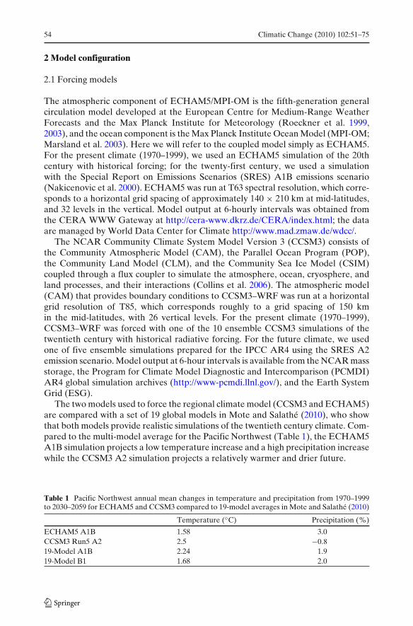
The two models used to force the regional climate model (CCSM3 and ECHAM5)are compared with a set of 19 global models in Mote and Salathé (2010), who showthat both models provide realistic simulations of the twentieth century climate. Com-pared to the multi-model average for the Pacific Northwest (Table 1), the ECHAM5A1B simulation projects a low temperature increase and a high precipitation increasewhile the CCSM3 A2 simulation projects a relatively warmer and drier future.

Table 1 Pacific Northwest annual mean changes in temperature and precipitation from 1970–1999to 2030–2059 for ECHAM5 and CCSM3 compared to 19-model averages in Mote and Salathé (2010)

Temperature (◦C) Precipitation (%)

ECHAM5 A1B 1.58 3.0CCSM3 Run5 A2 2.5 −0.819-Model A1B 2.24 1.919-Model B1 1.68 2.0

http://cera-www.dkrz.de/CERA/index.html

http://www.mad.zmaw.de/wdcc/

http://www-pcmdi.llnl.gov/


Since CCSM3 was run for an ensemble of simulations, we can compare thesimulation used here to the full ensemble. Differences among ensemble membersreflect the inherent variability in the simulated climate given the same radiativeforcing, and each simulation can be taken as an equally likely projection of theclimate. Of the parameters discussed here, precipitation shows by far the greatestvariation across the ensemble, consistent with the large observed natural variabilityin regional precipitation. While precipitation from the global model is not used inforcing the regional model, the winds and moisture fields are used, and this ensuresan overall compatibility of the global and regional precipitation simulation. Theensemble member used for this study (run 5) differs from the ensemble mean mostsignificantly in November precipitation over the Pacific Northwest. The CCSM3SRES A2 ensemble mean shows a modest increase in autumn and spring precipita-tion with decreases in the winter and summer, which is generally consistent with themulti-model ensemble mean discussed in Mote and Salathé (2010). For the ensemblemember used to force WRF, the 1970–1999 November mean Pacific Northwestprecipitation is the lowest and the 2030–2059 mean is the highest in the ensemble.Thus, the change in November precipitation is high compared to the ensemblemean. In the results below, we find that this increase in precipitation has a markedinfluence on the simulated regional climate change; these results must be inter-preted as the combined influence of systematic climate change and internal climatevariability.

2.2 Regional model

The WRF model is a state-of-the-art mesoscale numerical weather prediction systemdesigned to serve both operational forecasting and atmospheric research needs(http://www.wrf-model.org). This model has been developed and used extensivelyin recent years for regional climate simulation (Leung et al. 2006). WRF is a non-hydrostatic model with multiple choices for physical parameterizations suitablefor applications across scales ranging from meters to thousands of kilometers.The physics package includes microphysics, convective parameterization, planetaryboundary layer (PBL), land surface models (LSM), and longwave and shortwaveradiation.

In this work, the microphysics and convective parameterizations used were theWRF Single-Moment 5-class (WSM5) scheme (Hong et al. 2004) and the Kain–Fritsch scheme (Kain and Fritsch 1993). The WSM5 microphysics explicitly simulateswater vapor, cloud water, rain, cloud ice, and snow. The Kain–Fritsch convectiveparameterization utilizes a simple cloud model with moist updrafts and downdraftsthat includes the effects of detrainment and entrainment. The land-surface modelused was the NOAH (National Centers for Environmental Prediction—NCEP,Oregon State University, Air Force, and Hydrologic Research Lab) LSM (Chen andDudhia 2001). This is a four-layer soil temperature and moisture model with canopymoisture and snow cover prediction. It includes root zone, evapotranspiration, soildrainage, and runoff, taking into account vegetation categories, monthly vegetationfraction, and soil texture. A modification is included so that soil temperatures vary atthe lower boundary of the soil column (8-m depth) in accordance with the evolvingclimatological surface temperature. The PBL parameterization used was the YSU

http://www.wrf-model.org


(Yonsei University) scheme (Hong and Pan 1996). This scheme includes counter-gradient terms to represent heat and moisture fluxes due to both local and non-localgradients. Atmospheric shortwave and longwave radiation were computed by theNCAR CAM (Community Atmospheric Model) shortwave scheme and longwavescheme (Collins et al. 2004).

The most interesting differences between the ECHAM5–WRF and CCSM3–WRFsimulations are those due to the global model used to force the regional simulation.However, there are minor technical differences in the WRF model configurationsused at Pacific Northwest National Laboratory for the CCSM3–WRF and used at theUniversity of Washington for the ECHAM5–WRF simulations. First, the CCSM3–WRF simulation used the SRES A2 scenario while ECHAM5–WRF used the SRESA1B emissions scenario. The effect of these different emissions scenarios on thesimulated climate is minor since the two emissions scenarios do not begin to divergeuntil the mid twenty-first century. The difference between the PNW-mean annualwarming from 1970–1999 to 2030–2059 for the CCSM3 A2 simulation used for thispaper and the CCSM3 A1B simulation used in the remainder of the assessmentis less than 1◦C. Secondly, the ECHAM5–WRF simulation follows the methodsof the MM5-based mesoscale climate modeling described in Salathé et al. (2008):Nested grids and interior nudging are used to match the WRF simulation to theglobal model. The CCSM3–WRF uses a single model domain with a wider bufferzone for the lateral boundaries to increase the constraints from the global climatesimulation. The relaxation coefficients of the nudging boundary conditions followa linear-exponential function to smoothly blend the large-scale circulation fromthe global simulation and the regional simulation. As seen below, both simulationsclosely follow the forcing model, so both nudging and the extended buffer zone aresuccessful methods of constraining the regional simulation.

3 Model evaluation

To establish whether the regional climate simulations can reproduce the observedclimate of the Pacific Northwest, we compared the two simulations for the winter(December–January–February, DJF) and summer (June–July–August, JJA) to grid-ded observations averaged for the period 1970–1999, in a similar manner to Leunget al. (2003a, b). The gridded data consist of station observations interpolated to a1/16-degree grid using an empirical model for the effects of terrain on temperatureand precipitation (Daly et al. 1994; Elsner et al. 2010). Since the CCSM3 andECHAM5 simulations are from free-running climate models, the observed temporalsequence (i.e. at daily to interannual time scales) is not reproduced. However, foraverages over a period of 30 years, most natural and internal model variabilityshould be removed and we expect any differences among the simulations and griddedobservations to be the result of model deficiencies and, to some degree, differencesin grid resolutions.

It is important to note that a regional model does not explicitly remove any biasin the forcing model, except where such bias is due to unresolved processes, and mayintroduce additional biases. This comparison, therefore, evaluates both the regionalmodel and the global forcing model. Some uncertainty in the evaluation is introducedin using gridded observations as opposed to station observations since the gridding


procedure interpolates between the sparse station network based on a simple terrainmodel for temperature and precipitation.

An alternative method for evaluation of the WRF regional climate simulation,based on station observations, may be found in Zhang et al. (2009), who use thesame WRF implementation used for the ECHAM5–WRF simulations, but forcedby an atmospheric reanalysis, in order to isolate deficiencies in the mesoscale modelfrom errors in the forcing model. That study found that Tmax and Tmin simulated byWRF compare well with the station observations. Warm biases of Tmax are notedin WRF simulations between February and June with cold biases during the rest ofthe year. Warm biases of Tmin prevail throughout the year. The temporal correlationbetween the simulated and observed daily precipitation is low; however, the corre-lation increases steadily for longer averaging times, showing good representation ofseasonal and interannual variability.

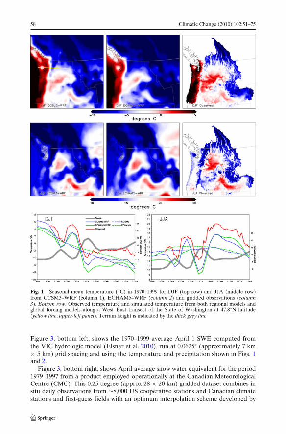
Figure 1 shows the winter (DJF) and summer (JJA) temperature simulatedby CCSM3–WRF (left) and ECHAM5–WRF (middle) simulation in compari-son to the gridded observations (right). The bottom two panels show simulatedand observed temperature and the ECHAM5–WRF terrain along a transect ofWashington at 47.8◦N; observed precipitation has been averaged over a latitude bandto reflect the model resolution. Overall, the temperature is well represented in thesimulations: the influence of the major geographical features is captured, and theseasonal cycle is reproduced. Both models exhibit a substantial cold bias relative tothe gridded observations. In DJF, this bias is evident over the Cascade crest andSoutheast Washington. Any bias in the global forcing models is inherited by theWRF simulation, so this comparison depends on combined deficiencies in the forcingmodel and regional model.

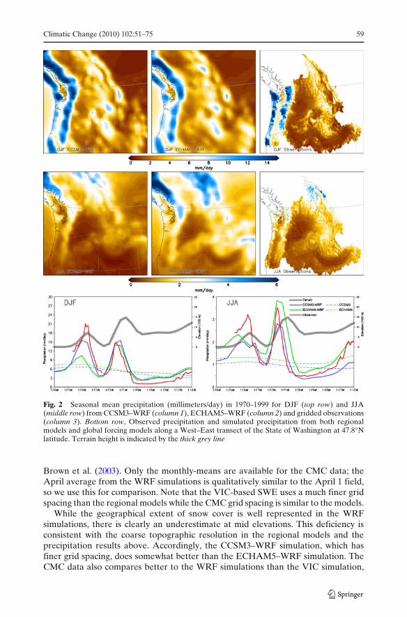
Figure 2 shows the corresponding results for simulated and observed 1970–1999precipitation. Again, the overall magnitude of precipitation and its geographicaldistribution are well characterized by the simulations for both seasons. Both modelsare unable to resolve the large precipitation peak over the Olympics, but do representthe maximum over the Cascades. The finer grid spacing in the CCSM3–WRFsimulation reproduces the intensity along the crests of the Cascades and Olympicsbetter than the ECHAM5–WRF simulation although precipitation is over estimatedin the southern Cascades of Oregon. Both models also do well in producing the peakprecipitation on the windward slopes of the Cascade Range with a rapid drop inthe lee. The CCSM3–WRF result produces comparable peaks for each range whilethe ECHAM5–WRF simulation produces a somewhat smaller maximum over theOlympics due to its coarser grid spacing. Compared to the Cascades, the Olympicsare lower elevation, have a smaller geographic extent, and are an isolated “hill” inthe models rather than a ridge as for the Cascades. As a result, finer grid spacingis required to simulate orographic precipitation over the Olympics than over theCascades. As shown in Leung and Qian (2003), as model resolution improves,the maximum over the Olympics becomes larger than that over the Cascades, inaccordance with observations.

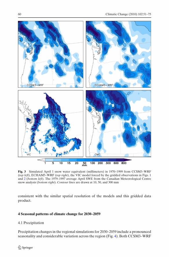
Figure 3, top panels, shows the 1970–1999 average April 1 snowpack from thetwo regional models expressed as millimeters of snow-water equivalent (SWE).SWE follow the spatial pattern of precipitation, with the CCSM3–WRF (left) clearlyshowing more tightly localized and higher SWE values than the ECHAM5–WRF(right) simulation. For comparison, we include two baseline snow climatologies.


Fig. 1 Seasonal mean temperature (◦C) in 1970–1999 for DJF (top row) and JJA (middle row)from CCSM3–WRF (column 1), ECHAM5–WRF (column 2) and gridded observations (column3). Bottom row, Observed temperature and simulated temperature from both regional models andglobal forcing models along a West–East transect of the State of Washington at 47.8◦N latitude(yellow line, upper-left panel). Terrain height is indicated by the thick grey line

Figure 3, bottom left, shows the 1970–1999 average April 1 SWE computed fromthe VIC hydrologic model (Elsner et al. 2010), run at 0.0625◦ (approximately 7 km× 5 km) grid spacing and using the temperature and precipitation shown in Figs. 1and 2.

Figure 3, bottom right, shows April average snow water equivalent for the period1979–1997 from a product employed operationally at the Canadian MeteorologicalCentre (CMC). This 0.25-degree (approx 28 × 20 km) gridded dataset combines insitu daily observations from ∼8,000 US cooperative stations and Canadian climatestations and first-guess fields with an optimum interpolation scheme developed by


Fig. 2 Seasonal mean precipitation (millimeters/day) in 1970–1999 for DJF (top row) and JJA(middle row) from CCSM3–WRF (column 1), ECHAM5–WRF (column 2) and gridded observations(column 3). Bottom row, Observed precipitation and simulated precipitation from both regionalmodels and global forcing models along a West–East transect of the State of Washington at 47.8◦Nlatitude. Terrain height is indicated by the thick grey line

Brown et al. (2003). Only the monthly-means are available for the CMC data; theApril average from the WRF simulations is qualitatively similar to the April 1 field,so we use this for comparison. Note that the VIC-based SWE uses a much finer gridspacing than the regional models while the CMC grid spacing is similar to the models.

While the geographical extent of snow cover is well represented in the WRFsimulations, there is clearly an underestimate at mid elevations. This deficiency isconsistent with the coarse topographic resolution in the regional models and theprecipitation results above. Accordingly, the CCSM3–WRF simulation, which hasfiner grid spacing, does somewhat better than the ECHAM5–WRF simulation. TheCMC data also compares better to the WRF simulations than the VIC simulation,


Fig. 3 Simulated April 1 snow water equivalent (millimeters) in 1970–1999 from CCSM3–WRF(top left), ECHAM5–WRF (top right), the VIC model forced by the gridded observations in Figs. 1and 2 (bottom left). The 1979–1997 average April SWE from the Canadian Meteorological Centresnow analysis (bottom right). Contour lines are drawn at 10, 50, and 300 mm

consistent with the similar spatial resolution of the models and this gridded dataproduct.

4 Seasonal patterns of climate change for 2030–2059

4.1 Precipitation

Precipitation changes in the regional simulations for 2030–2059 include a pronouncedseasonality and considerable variation across the region (Fig. 4). Both CCSM3–WRF


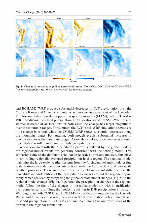
Fig. 4 Change in precipitation (millimeters/month) from 1970–1999 to 2030–2059 for CCSM3–WRF(top row) and ECHAM5–WRF (bottom row) for the four seasons

and ECHAM5–WRF produce substantial decreases in DJF precipitation over theCascade Range and Olympic Mountains and modest increases east of the Cascades.The two simulations produce opposite responses in spring (MAM), with ECHAM5–WRF producing increased precipitation at all locations and CCSM3–WRF a sub-stantial decrease at all locations; in both cases the change has larger magnitudesover the mountain ranges. For summer, the ECHAM5–WRF simulation shows verylittle change in rainfall while the CCSM3–WRF shows substantial decreases alongthe mountain ranges. For autumn, both models predict substantial increases inprecipitation over the mountain ranges. As we show below, the increases in autumnprecipitation result in more intense daily precipitation events.

When compared with the precipitation pattern simulated by the global models,the regional model results are generally consistent with the forcing model. Thissimilarity is due to the dominant role that large-scale storms and moisture flux playsin controlling regionally averaged precipitation in this region. The regional modelmaintains the large-scale weather systems from the forcing model and simulates finescale features that derive from interactions with the land surface and mesoscaleweather processes. These mesoscale processes yield important differences in themagnitude and distribution of the precipitation changes around the regional topog-raphy, which are seen by comparing the global climate model changes (Fig. 5) to theregional model changes (Fig. 4). In general, the precipitation changes in the regionalmodel follow the sign of the changes in the global model but with intensificationover complex terrain. Thus, the modest reduction in DJF precipitation in westernWashington in both CCSM3 and ECHAM5 is considerably amplified in the CascadeRange and Olympics. Likewise, increases in SON precipitation in both models andin MAM precipitation in ECHAM5 are amplified along the windward sides of theterrain in the regional simulations.


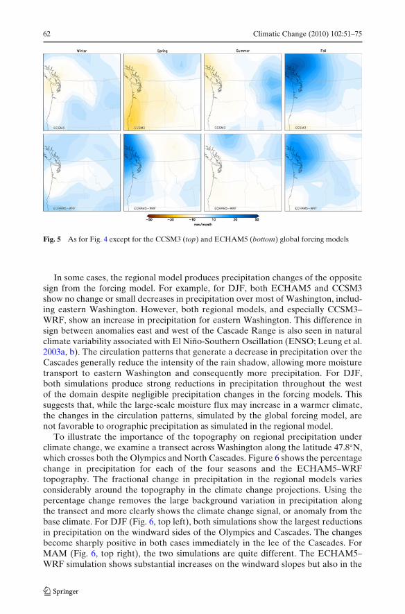
Fig. 5 As for Fig. 4 except for the CCSM3 (top) and ECHAM5 (bottom) global forcing models

In some cases, the regional model produces precipitation changes of the oppositesign from the forcing model. For example, for DJF, both ECHAM5 and CCSM3show no change or small decreases in precipitation over most of Washington, includ-ing eastern Washington. However, both regional models, and especially CCSM3–WRF, show an increase in precipitation for eastern Washington. This difference insign between anomalies east and west of the Cascade Range is also seen in naturalclimate variability associated with El Niño-Southern Oscillation (ENSO; Leung et al.2003a, b). The circulation patterns that generate a decrease in precipitation over theCascades generally reduce the intensity of the rain shadow, allowing more moisturetransport to eastern Washington and consequently more precipitation. For DJF,both simulations produce strong reductions in precipitation throughout the westof the domain despite negligible precipitation changes in the forcing models. Thissuggests that, while the large-scale moisture flux may increase in a warmer climate,the changes in the circulation patterns, simulated by the global forcing model, arenot favorable to orographic precipitation as simulated in the regional model.

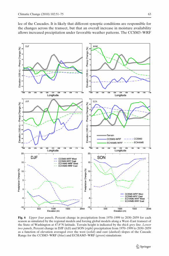
To illustrate the importance of the topography on regional precipitation underclimate change, we examine a transect across Washington along the latitude 47.8◦N,which crosses both the Olympics and North Cascades. Figure 6 shows the percentagechange in precipitation for each of the four seasons and the ECHAM5–WRFtopography. The fractional change in precipitation in the regional models variesconsiderably around the topography in the climate change projections. Using thepercentage change removes the large background variation in precipitation alongthe transect and more clearly shows the climate change signal, or anomaly from thebase climate. For DJF (Fig. 6, top left), both simulations show the largest reductionsin precipitation on the windward sides of the Olympics and Cascades. The changesbecome sharply positive in both cases immediately in the lee of the Cascades. ForMAM (Fig. 6, top right), the two simulations are quite different. The ECHAM5–WRF simulation shows substantial increases on the windward slopes but also in the


lee of the Cascades. It is likely that different synoptic conditions are responsible forthe changes across the transect, but that an overall increase in moisture availabilityallows increased precipitation under favorable weather patterns. The CCSM3–WRF

Fig. 6 Upper four panels, Percent change in precipitation from 1970–1999 to 2030–2059 for eachseason as simulated by the regional models and forcing global models along a West–East transect ofthe State of Washington at 47.8◦N latitude. Terrain height is indicated by the thick grey line. Lowertwo panels, Percent change in DJF (left) and SON (right) precipitation from 1970–1999 to 2030–2059as a function of elevation averaged over the west (solid) and east (dashed) slopes of the CascadeRange for the CCSM3–WRF (blue) and ECHAM5–WRF (green) simulations


simulation shows a more uniform decrease in precipitation, with a maximum on thewindward slope of the Olympics. Results for both models in SON (Fig. 6, bottomright) are similar to the MAM results for ECHAM5–WRF. Peak precipitationincreases are found not only on the windward slopes, but also in Eastern Washington,where the fractional increase is comparable to the increases over the mountains.

Another way to view these results is to consider the changes in precipitation withelevation on the windward (west) and lee (east) slopes of the Cascades. To make thiscomparison, the percent change in precipitation from the current to future simulationwas computed along the entire range in Washington for each side of the crest. Thesewere then averaged in 200-m elevation bands. Results for DJF and SON are shownin Fig. 6, bottom row. Consistent with the transect results, decreases are found overthe western slopes for both simulations. For CCSM3–WRF, the decrease diminishes,becoming a substantial increase, moving down slope east of the crest. ECHAM5–WRF projects relatively small and uniform increases in precipitation east of thecrest. In both cases, these changes represent a weakening of the climatological rainshadow. Leung et al. (2003a, b) suggest that the weakening of the rain shadow isgenerally associated with changes in the circulation patterns, such as winds shiftingto a direction more parallel rather than perpendicular to the dominant ridge, thatweaken orographic enhancement. Although the percentage increase on the lee sidecan be comparable to the decrease on the windward side, the net change in regionwide precipitation, which is important for large river basin runoff, is a net increasebecause precipitation on the upwind slope is significantly higher than that in the rainshadow. For SON, the simulated changes across the Cascades are quite different,with increases on both slopes. The increase is largest on the windward slope,especially for the CCSM3–WRF simulation. Stronger orographic enhancement alonewould tend to decrease precipitation on the lee, so this result suggests a combinationof changes in moisture availability or moisture source and orographic enhancementare responsible for the simulated changes.

These results give clear evidence that the effect of climate change on precipitationis tightly coupled to the interaction of increased moisture availability and varioussynoptic weather patterns with the regional topography.

4.2 Temperature

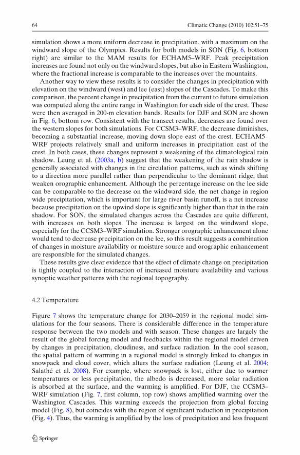
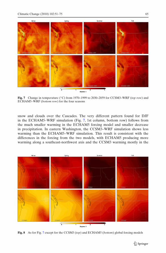
Figure 7 shows the temperature change for 2030–2059 in the regional model sim-ulations for the four seasons. There is considerable difference in the temperatureresponse between the two models and with season. These changes are largely theresult of the global forcing model and feedbacks within the regional model drivenby changes in precipitation, cloudiness, and surface radiation. In the cool season,the spatial pattern of warming in a regional model is strongly linked to changes insnowpack and cloud cover, which alters the surface radiation (Leung et al. 2004;Salathé et al. 2008). For example, where snowpack is lost, either due to warmertemperatures or less precipitation, the albedo is decreased, more solar radiationis absorbed at the surface, and the warming is amplified. For DJF, the CCSM3–WRF simulation (Fig. 7, first column, top row) shows amplified warming over theWashington Cascades. This warming exceeds the projection from global forcingmodel (Fig. 8), but coincides with the region of significant reduction in precipitation(Fig. 4). Thus, the warming is amplified by the loss of precipitation and less frequent


Fig. 7 Change in temperature (◦C) from 1970–1999 to 2030–2059 for CCSM3–WRF (top row) andECHAM5–WRF (bottom row) for the four seasons

snow and clouds over the Cascades. The very different pattern found for DJFin the ECHAM5–WRF simulation (Fig. 7, 1st column, bottom row) follows fromthe much smaller warming in the ECHAM5 forcing model and smaller decreasein precipitation. In eastern Washington, the CCSM3–WRF simulation shows lesswarming than the ECHAM5–WRF simulation. This result is consistent with thedifferences in the forcing from the two models, with ECHAM5 producing morewarming along a southeast-northwest axis and the CCSM3 warming mostly in the

Fig. 8 As for Fig. 7 except for the CCSM3 (top) and ECHAM5 (bottom) global forcing models


eastern portion of the domain. Furthermore, precipitation increases over easternWashington in the CCSM3–WRF simulation, which implies increased cloud coverand reduced solar heating of the surface.

For MAM (Fig. 7, 2nd column), the differences between the two simulations seenfor DJF are accentuated due to the very different precipitation results, with consider-able loss of precipitation in CCSM3–WRF and considerable increase in ECHAM5–WRF. For JJA, both regional models closely follow the global model, which suggeststhat mesoscale processes are not as critical to the summer temperature sensitivity.In spring and summer, both the global and regional models indicate less warmingin coastal areas than inland. In some cases, the regional models reduce the coastalwarming relative to the global model. Nevertheless, warming is still substantial inwestern Washington and, as shown below, heat waves are projected to become morefrequent. For SON, the global forcing models and regional precipitation response arevery similar and thus the temperature changes are similar.

4.3 Snowpack

Substantial losses of snowpack are found in both regional simulations. Figure 9shows the change in average spring (MAM) snowpack from the present to futureclimate. When averaged over Washington, CCSM3–WRF projects a 71% loss ofSWE while ECHAM5–WRF projects a 32% loss. Since spring snowpack is a goodpredictor of summertime streamflows, changes for this season indicate the magnitudeof the impacts of regional climate change on water resources (see Vano et al.2010). The CCSM3–WRF simulation (Fig. 9, left) yields much larger snow lossthan ECHAM5–WRF (Fig. 9, right) over the entire domain, but particularly for theCascade and Olympic mountains. In part, this may be due to the finer grid spacing

Fig. 9 Change in April 1 snow water equivalent (millimeters) from CCSM3–WRF (left) andECHAM5–WRF (right)


in CCSM3–WRF, allowing better representation of smaller terrain features such asthe Olympics. However, the 1970–1999 snowpack (Fig. 3) is more similar betweenthe two models than the simulated changes, so model resolution is not the mostimportant effect.

Most of the difference between the two simulations is due to the forcing modelsand the resulting regional precipitation. Snowpack changes are a result of bothchanges in precipitation and changes in temperature (Mote et al. 2008). WhileCCSM3–WRF show somewhat more warming than ECHAM5–WRF and bothmodels show increased autumn precipitation, the dominant effect on the differencesin simulated spring snowpack is the difference in precipitation projections. Figure 4shows a larger reduction in winter and spring precipitation in CCSM3–WRF thanin ECHAM5–WRF, and this result dominates the snowpack results. The consensusamong global climate models (Mote and Salathé 2010) is for modest increases incool-season precipitation, so the CCSM3 results presented here are not necessarilycharacteristic. Nevertheless, despite the increase in cool-season precipitation inECHAM5–WRF, snowpack decreases over a similar geographical extent as in themuch drier CCSM3–WRF projection and about half the magnitude. Thus, while thedisparity in precipitation projections in the two models modulates the magnitudeof snow loss, warming plays a prominent role in determining future snowpack,counteracting potential increases in precipitation.

The ECHAM5–WRF and CCSM3–WRF projections for cool-season (November–March) changes in temperature and precipitation and for changes in April 1 SWE aregiven in Table 1. These may be compared to the results from Elsner et al. (2010)and Casola et al. (2009) as follows. Casola et al. (2009), using simple theoreticalarguments, estimate a 16% loss of snowpack for each 1◦C of warming. This estimateassumes a 5% increase in precipitation for each degree of warming. These values maybe estimated directly from the data in Elsner et al. (2010) based on computationsusing a hydrologic model and perturbed historic temperature and precipitation data.From their Tables 4 and 6 for the three time periods and two emissions projections,the loss in SWE ranges between 20.3% and 27% per 1◦C of warming, with an averageof 24.6% per 1◦C. The multi-model average results show consistent precipitationincreases with temperature, ranging from 2.1 to 3.3 per 1◦C, with an average of 2.8%per 1◦C. Our results show a much larger sensitivity of SWE to temperature than inCasola et al. (2009). In part, this is due to the much smaller increases in precipitationwith temperature simulated by the climate models than the 5% they assumed, but thisonly accounts for a few percentage points. An important difference between the twostudies is that Casola et al. (2009) consider only the Puget Sound basin, consistingmainly of the western slopes of the Cascade Range while Elsner et al. (2010) andthis study consider the entire state of Washington. It is not immediately clear howthe larger domain would affect the sensitivity, however it is likely that the easternportion of the domain, with significant mid-elevation snowpack, would have greatersensitivity than the Puget Sound basin.

To estimate the change in SWE from these relationships using the WRF temper-ature and precipitation results, we use the temperature change to obtain an initialSWE change and a predicted precipitation change. Since the WRF projections forprecipitation do not match the simple assumptions in Casola et al. (2009) nor themulti-model mean in Elsner et al. (2010), we apply a correction based on the overor under estimate of precipitation relative to the WRF simulation. The correction is


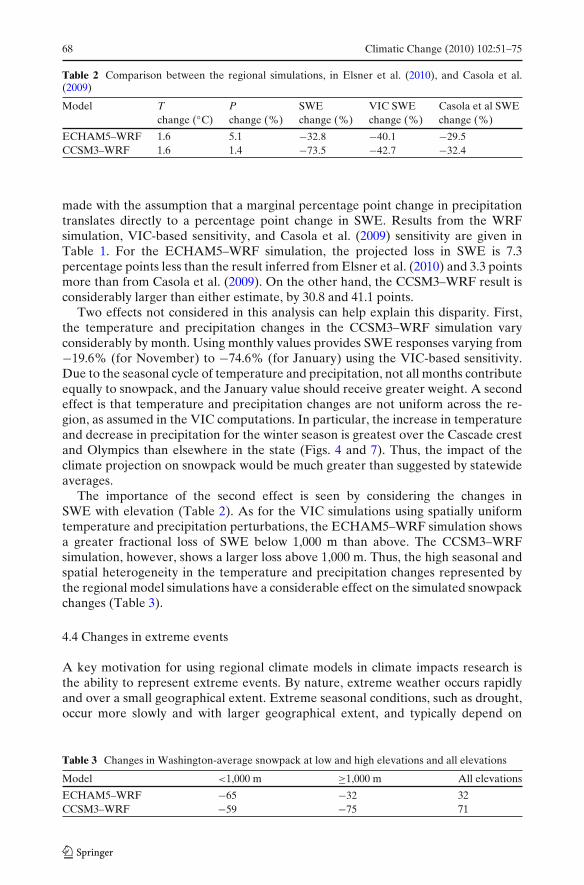
Table 2 Comparison between the regional simulations, in Elsner et al. (2010), and Casola et al.(2009)

Model T P SWE VIC SWE Casola et al SWEchange (◦C) change (%) change (%) change (%) change (%)

ECHAM5–WRF 1.6 5.1 −32.8 −40.1 −29.5CCSM3–WRF 1.6 1.4 −73.5 −42.7 −32.4

made with the assumption that a marginal percentage point change in precipitationtranslates directly to a percentage point change in SWE. Results from the WRFsimulation, VIC-based sensitivity, and Casola et al. (2009) sensitivity are given inTable 1. For the ECHAM5–WRF simulation, the projected loss in SWE is 7.3percentage points less than the result inferred from Elsner et al. (2010) and 3.3 pointsmore than from Casola et al. (2009). On the other hand, the CCSM3–WRF result isconsiderably larger than either estimate, by 30.8 and 41.1 points.

Two effects not considered in this analysis can help explain this disparity. First,the temperature and precipitation changes in the CCSM3–WRF simulation varyconsiderably by month. Using monthly values provides SWE responses varying from−19.6% (for November) to −74.6% (for January) using the VIC-based sensitivity.Due to the seasonal cycle of temperature and precipitation, not all months contributeequally to snowpack, and the January value should receive greater weight. A secondeffect is that temperature and precipitation changes are not uniform across the re-gion, as assumed in the VIC computations. In particular, the increase in temperatureand decrease in precipitation for the winter season is greatest over the Cascade crestand Olympics than elsewhere in the state (Figs. 4 and 7). Thus, the impact of theclimate projection on snowpack would be much greater than suggested by statewideaverages.

The importance of the second effect is seen by considering the changes inSWE with elevation (Table 2). As for the VIC simulations using spatially uniformtemperature and precipitation perturbations, the ECHAM5–WRF simulation showsa greater fractional loss of SWE below 1,000 m than above. The CCSM3–WRFsimulation, however, shows a larger loss above 1,000 m. Thus, the high seasonal andspatial heterogeneity in the temperature and precipitation changes represented bythe regional model simulations have a considerable effect on the simulated snowpackchanges (Table 3).

4.4 Changes in extreme events

A key motivation for using regional climate models in climate impacts research isthe ability to represent extreme events. By nature, extreme weather occurs rapidlyand over a small geographical extent. Extreme seasonal conditions, such as drought,occur more slowly and with larger geographical extent, and typically depend on

Table 3 Changes in Washington-average snowpack at low and high elevations and all elevations

Model <1,000 m ≥1,000 m All elevations

ECHAM5–WRF −65 −32 32CCSM3–WRF −59 −75 71


fine-scale interactions between the atmosphere and land surface features such astopography that are not well resolved in global models. Thus, regional climatemodels are especially well suited to studying these events. Here we present summarystatistics for several types of extreme events related to temperature and precipitation.Our analysis follows the approach of Tebaldi et al. (2006) for global climate modelanalysis and uses parameters defined in Frich et al. (2002).

4.5 Heat waves and warm nights

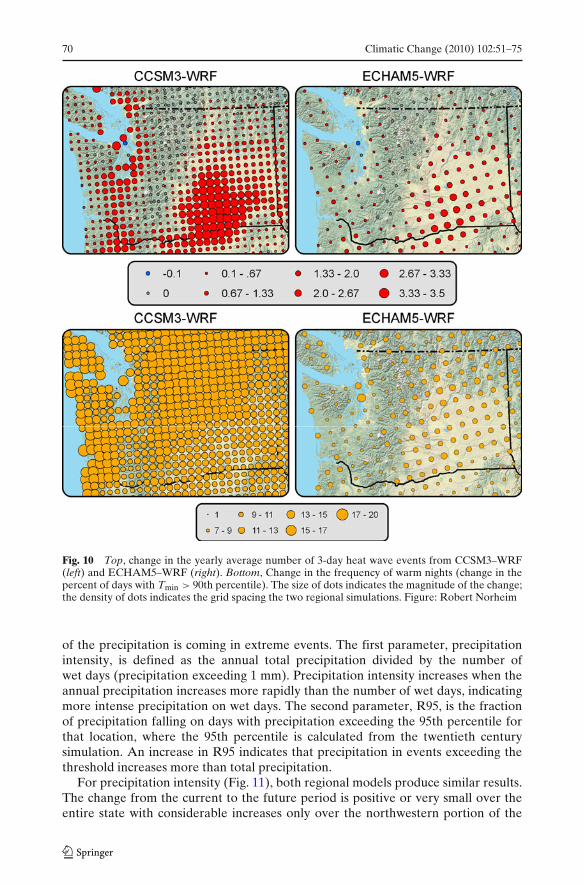
Climate change is predicted to have significant human health consequences dueto heat stress in vulnerable individuals. This issue is discussed in detail in Jacksonet al. (2010) where the quantitative relationship between heat events and mortality isanalyzed, showing that mortality rises significantly after heat waves last for three ormore days. Future heat wave frequencies are represented in Jackson et al. (2010)by a uniform perturbation to the historic record since the global climate modelsdo not give good information on the geographic signature of warming or changesin daily variability. Here we use output from the regional models to compute thefrequency of heat waves for present and future time periods. We define a heatwave as an episode of three or more days where the daily heat index (Humidex)exceeds 32◦C. Figure 10, top panel, shows the change in the yearly average numberof heat waves of 3-day duration simulated by the two regional models from 1970–1999 to 2030–2059. Both models show a larger increase in heat wave frequencyin south-central Washington than elsewhere in the state, with up to 3 more heatwaves each year in the future period than in the control period. The CCSM3–WRF simulation (Fig. 10, left) also shows considerable increase in heat waves inthe lowlands of western Washington, following the more widespread warming in theCCSM3 scenario. Note that this increase in heat waves occurs despite relatively lessseasonal-average warming here than the interior. This result suggests that effects thatwould moderate coastal warming, such as marine cloudiness, are intermittent andhave little effect on the frequency and duration of extreme heat events. Althoughthe heat index includes the effect of relative humidity, the large increase in heat wavefrequency in south-central Washington is a result of an increase only in temperaturesince summertime relative humidity remains nearly constant for this region underclimate change.

The frequency of warm nights is another measure of persistent heat stress withimportant impacts. To analyze the change in the frequency of warm nights, wecomputed the 90th percentile minimum temperature (Tmin) for each calendar day ateach grid point for the twentieth century simulations. The change in the percentageof days where Tmin exceeds the twentieth century’s 90th percentile is then computedfrom the twenty-first century simulation as shown in Fig. 10, bottom panel. Incomparison to the change in heat-wave frequency, the frequency of warm nights doesnot show as marked a geographical pattern, but rather closely follows the pattern ofsummertime warming (Fig. 7).

4.6 Extreme precipitation

We use two parameters to analyze changes in extreme precipitation, which yieldsomewhat different results. An increase in these parameters indicates that more


Fig. 10 Top, change in the yearly average number of 3-day heat wave events from CCSM3–WRF(left) and ECHAM5–WRF (right). Bottom, Change in the frequency of warm nights (change in thepercent of days with Tmin > 90th percentile). The size of dots indicates the magnitude of the change;the density of dots indicates the grid spacing the two regional simulations. Figure: Robert Norheim

of the precipitation is coming in extreme events. The first parameter, precipitationintensity, is defined as the annual total precipitation divided by the number ofwet days (precipitation exceeding 1 mm). Precipitation intensity increases when theannual precipitation increases more rapidly than the number of wet days, indicatingmore intense precipitation on wet days. The second parameter, R95, is the fractionof precipitation falling on days with precipitation exceeding the 95th percentile forthat location, where the 95th percentile is calculated from the twentieth centurysimulation. An increase in R95 indicates that precipitation in events exceeding thethreshold increases more than total precipitation.

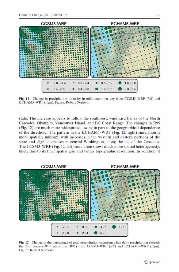
For precipitation intensity (Fig. 11), both regional models produce similar results.The change from the current to the future period is positive or very small over theentire state with considerable increases only over the northwestern portion of the


Fig. 11 Change in precipitation intensity in millimeters per day from CCSM3–WRF (left) andECHAM5–WRF (right). Figure: Robert Norheim

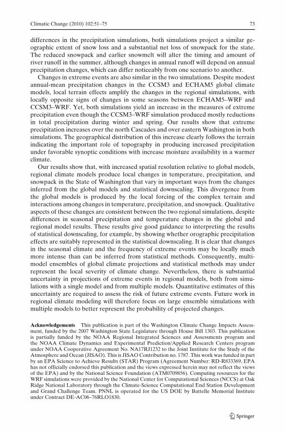
state. The increase appears to follow the southwest, windward flanks of the NorthCascades, Olympics, Vancouver Island, and BC Coast Range. The changes in R95(Fig. 12) are much more widespread, owing in part to the geographical dependenceof the threshold. The pattern in the ECHAM5–WRF (Fig. 12, right) simulation ismore spatially uniform, with increases in the western and eastern portions of thestate and slight decreases in central Washington, along the lee of the Cascades.The CCSM3–WRF (Fig. 12, left) simulation shows much more spatial heterogeneity,likely due to its finer spatial grid and better topographic resolution. In addition, it

Fig. 12 Change in the percentage of total precipitation occurring when daily precipitation exceedsthe 20th century 95th percentile (R95) from CCSM3–WRF (left) and ECHAM5–WRF (right).Figure: Robert Norheim


is interesting to note that in CCSM3–WRF, both precipitation intensity and R95increase substantially on the windward slopes of the coastal mountains despitereductions in the total annual precipitation shown in Fig. 4.

As discussed above, the CCSM3 ensemble member used to force the CCSM3–WRF simulation has an uncharacteristic increase in November precipitation. Totest how critical this result is in determining the change in extreme precipitation,we repeated the above analysis using only data for the months December throughFebruary. This restriction makes very little difference for the ECHAM5–WRFsimulation, although there is a more pronounced reduction in extremes along thelee of the Cascade Range and a larger increase elsewhere. For the CCSM3–WRFsimulation, the increase in extremes for western Washington remains but is reduced;the increase east of the Cascade Range, however, is amplified. Qualitatively, theresults based on all months are consistent with the results for the winter months,with some geographical differences.

Consistent with previous findings (e.g., Leung et al. 2004), these results sug-gest that extreme precipitation changes are more related to increased moistureavailability in a warmer climate than to increases in climate-mean precipitation.Although changes in the mean large-scale circulation may not favor precipitation in aclimatological sense, increased atmospheric moisture availability under intermittentsynoptic conditions favorable for precipitation can lead to increased precipitationintensity and extreme precipitation. This finding has important implications as itsuggests that extreme precipitation can increase regardless of the change in totalprecipitation, which has larger uncertainty as shown in Fig. 4.

5 Conclusion

Regional climate models provide important insight into how the regional climatemay respond to global climate change. We have presented two long simulationsfrom a mesoscale climate model forced by two global climate model simulations. Theobject of regional climate modeling is to understand how fine scale weather and land-surface processes respond to the large-scale forcing generated by global models, andhow that may alter the local climate change patterns. In overall details, both simula-tions presented here are quite consistent with the global forcing models used, whichis expected. Furthermore, due to the unique characteristics of the forcing models,the fine scale features simulated are substantially different, accentuating differencesin the forcing scenarios and underscoring the need for extended simulations using alarge ensemble of forcing models and regional models.

The most profound difference between the two simulations is in the cool-seasonprecipitation, which is closely related to the simulated changes in snow pack andtemperature. The CCSM3–WRF model shows substantial decreases in winter andspring precipitation. This, combined with a strong warming signal, yields substantialdecreases in snow pack along the Cascade Crest and Olympic mountains. Wheresnow cover is reduced, the warming is locally amplified, suggesting a feedbackbetween precipitation, snowpack, and temperature.

Despite these differences, there are important areas of agreement between thetwo simulations, suggesting that some local responses to global climate change arerobust. Most clear is the loss of snowpack in both simulations. Despite substantial


differences in the precipitation simulations, both simulations project a similar ge-ographic extent of snow loss and a substantial net loss of snowpack for the state.The reduced snowpack and earlier snowmelt will alter the timing and amount ofriver runoff in the summer, although changes in annual runoff will depend on annualprecipitation changes, which can differ noticeably from one scenario to another.

Changes in extreme events are also similar in the two simulations. Despite modestannual-mean precipitation changes in the CCSM3 and ECHAM5 global climatemodels, local terrain effects amplify the changes in the regional simulations, withlocally opposite signs of changes in some seasons between ECHAM5–WRF andCCSM3–WRF. Yet, both simulations yield an increase in the measures of extremeprecipitation even though the CCSM3–WRF simulation produced mostly reductionsin total precipitation during winter and spring. Our results show that extremeprecipitation increases over the north Cascades and over eastern Washington in bothsimulations. The geographical distribution of this increase clearly follows the terrainindicating the important role of topography in producing increased precipitationunder favorable synoptic conditions with increase moisture availability in a warmerclimate.

Our results show that, with increased spatial resolution relative to global models,regional climate models produce local changes in temperature, precipitation, andsnowpack in the State of Washington that vary in important ways from the changesinferred from the global models and statistical downscaling. This divergence fromthe global models is produced by the local forcing of the complex terrain andinteractions among changes in temperature, precipitation, and snowpack. Qualitativeaspects of these changes are consistent between the two regional simulations, despitedifferences in seasonal precipitation and temperature changes in the global andregional model results. These results give good guidance to interpreting the resultsof statistical downscaling, for example, by showing whether orographic precipitationeffects are suitably represented in the statistical downscaling. It is clear that changesin the seasonal climate and the frequency of extreme events may be locally muchmore intense than can be inferred from statistical methods. Consequently, multi-model ensembles of global climate projections and statistical methods may underrepresent the local severity of climate change. Nevertheless, there is substantialuncertainty in projections of extreme events in regional models, both from simu-lations with a single model and from multiple models. Quantitative estimates of thisuncertainty are required to assess the risk of future extreme events. Future work inregional climate modeling will therefore focus on large ensemble simulations withmultiple models to better represent the probability of projected changes.

Acknowledgements This publication is part of the Washington Climate Change Impacts Assess-ment, funded by the 2007 Washington State Legislature through House Bill 1303. This publicationis partially funded by the NOAA Regional Integrated Sciences and Assessments program andthe NOAA Climate Dynamics and Experimental Prediction/Applied Research Centers programunder NOAA Cooperative Agreement No. NA17RJ1232 to the Joint Institute for the Study of theAtmosphere and Ocean (JISAO). This is JISAO Contribution no. 1787. This work was funded in partby an EPA Science to Achieve Results (STAR) Program (Agreement Number: RD-R833369, EPAhas not officially endorsed this publication and the views expressed herein may not reflect the viewsof the EPA) and by the National Science Foundation (ATM0709856). Computing resources for theWRF simulations were provided by the National Center for Computational Sciences (NCCS) at OakRidge National Laboratory through the Climate-Science Computational End Station Developmentand Grand Challenge Team. PNNL is operated for the US DOE by Battelle Memorial Instituteunder Contract DE-AC06–76RLO1830.


References

Brown RD, Brasnett B, Robinson D (2003) Gridded North American monthly snow depth and snowwater equivalent for GCM evaluation. Atmos Ocean 41:1–14

Casola JH, Cuo L, Livneh B, Lettenmaier DP, Stoelinga MT, Mote PW, Wallace JM (2009) Assessingthe impacts of global warming on snowpack in the Washington cascades. J Climate 22:2758–2772

Chen F, Dudhia J (2001) Coupling an advanced land surface-hydrology model with the Penn State-NCAR MM5 modeling system. Part I: model implementation and sensitivity. Mon Weather Rev129:569–585

Collins WD, Rasch PJ, Boville BA, Hack JJ, McCaa JR, Williamson DL, Kiehl JT, Briegleb B,Bitz C, Lin S-J, Zhang M, Dai Y (2004) Description of the NCAR community atmospheric model(CAM 3.0). NCAR Tech. Note, NCAR/TN-464+STR, 226

Collins W et al (2006) The community climate system model version 3 (CCSM3). J Climate 19:2122–2143

Daly C, Neilson RP, Phillips DL (1994) A statistical topographic model for mapping climatologicalprecipitation over mountainous terrain. J Appl Meteorol 33:140–158

Elsner MM, Cuo L, Voisin N, Deems JS, Hamlet AF, Vano JA, Mickelson KEB, Lee SY,Lettenmaier DP (2010) Implications of 21st century climate change for the hydrology ofWashington State. Clim Change. doi:10.1007/s10584-010-9855-0

Frich P, Alexander LV, Della-Marta P, Gleason B, Haylock M, Tank A, Peterson T (2002) Observedcoherent changes in climatic extremes during the second half of the twentieth century. Clim Res19:193–212

Giorgi F, Mearns LO (1999) Introduction to special section: regional climate modeling revisited.J Geophys Res-Atmos 104:6335–6352

Hong SY, Pan HL (1996) Nonlocal boundary layer vertical diffusion in a medium-range forecastmodel. Mon Weather Rev 124:2322–2339

Hong SY, Dudhia J, Chen SH (2004) A revised approach to ice microphysical processes for the bulkparameterization of clouds and precipitation. Mon Weather Rev 132:103–120

Jackson JE, Yost MG, Karr C, Fitzpatrick C, Lamb BK, Chung S, Chen J, Avise J,Rosenblatt RA, Fenske RA (2010) Public health impacts of climate change in WashingtonState: projected mortality risks due to heat events and air pollution. Clim Change. doi:10.1007/s10584-010-9852-3

Kain JS, Fritsch JM (1993) Convective parameterization for mesoscale models: the Kain–Fritschscheme. In: Emanuel KA, Raymond DJ (eds) The representation of cumulus convection innumerical models. American Meteorological Society, Boston, pp 165–170

Leung LR, Qian Y (2003) The sensitivity of precipitation and snowpack simulations to modelresolution via nesting in regions of complex terrain. J Hydrometeorol 4:1025–1043

Leung LR, Qian Y, Bian X (2003a) Hydroclimate of the western United States based on observationsand regional climate simulation of 1981–2000. Part I: seasonal statistics. J Climate 16:1892–1911

Leung LR, Qian Y, Bian X, Hunt A (2003b) Hydroclimate of the western United States based onobservations and regional climate simulation of 1981–2000. Part II: mesoscale ENSO anomalies.J Climate 16:1912–1928

Leung LR, Qian Y, Bian X, Washington WM, Han J, Roads JO (2004) Mid-century ensembleregional climate change scenarios for the western United States. Clim Change 62:75–113

Leung LR, Kuo YH, Tribbia J (2006) Research needs and directions of regional climate modelingusing WRF and CCSM. B Am Meteorol Soc 87:1747–1751

Marsland SJ, Haak H, Jungclaus JH, Latif M, Roske F (2003) The Max–Planck institute globalocean/sea ice model with orthogonal curvilinear coordinates. Ocean Model 5:91–127

Mote PW, Salathé EP Jr (2010) Future climate in the Pacific Northwest. Clim Change. doi:10.1007/s10584-010-9848-z

Mote PW, Hamlet AF, Salathé EP (2008) Has spring snowpack declined in the Washington cascades?Hydrol Earth Syst Sci 12:193–206

Nakicenovic N et al (2000) IPCC special report on emissions scenarios. Cambridge University Press,Cambridge

Roeckner E, Bengtsson L, Feichter J, Lelieveld J, Rodhe H (1999) Transient climate change simula-tions with a coupled atmosphere-ocean GCM including the tropospheric sulfur cycle. J Climate12:3004–3032

Roeckner E, Bäuml G, Bonaventura L, Brokopf R, Esch M, Giorgetta M, Hagemann S,Kirchner I, Kornbleuh L, Manzini E, Rhodin A, Schlese U, Schulzweida U, Tomkins A (2003)

http://dx.doi.org/10.1007/s10584-010-9855-0

http://dx.doi.org/10.1007/s10584-010-9852-3

http://dx.doi.org/10.1007/s10584-010-9852-3

http://dx.doi.org/10.1007/s10584-010-9848-z

http://dx.doi.org/10.1007/s10584-010-9848-z


The atmospheric general circulation model ECHAM5, Part I: model description, Max–PlanckInstitute for Meteorology Report No. 349

Rosenberg EA, Keys PW, Booth DB, Hartley D, Burkey J, Steinemann AC, Lettenmaier DP(2010) Precipitation extremes and the impacts of climate change on stormwater infrastructurein Washington State. Clim Change. doi:10.1007/s10584-010-9847-0

Salathé EP (2003) Comparison of various precipitation downscaling methods for the simulation ofstreamflow in a rainshadow river basin. Int J Climatol 23:887–901

Salathé EP (2005) Downscaling simulations of future global climate with application to hydrologicmodeling. Int J Climatol 25:419–436

Salathé EP, Steed R, Mass CF, Zahn P (2008) A high-resolution climate model for the U.S. PacificNorthwest: mesoscale feedbacks and local responses to climate change. J Climatol 21:5708–5726

Tebaldi C, Hayhoe K, Arblaster JM, Meehl GA (2006) Going to the extremes. Clim Change79:185–211

Vano JA, Voisin N, Cuo L, Hamlet AF, Elsner MM, Palmer RN, Polebitski A, Lettenmaier DP(2010) Climate change impacts on water management in the Puget Sound region, Washington,USA. Clim Change. doi:10.1007/s10584-010-9846-1

Widmann M, Bretherton CS, Salathé EP (2003) Statistical precipitation downscaling over theNorthwestern United States using numerically simulated precipitation as a predictor. J Climatol16:799–816

Wood AW, Leung LR, Sridhar V, Lettenmaier DP (2004) Hydrologic implications of dynamical andstatistical approaches to downscaling climate model outputs. Clim Change 62:189–216

Zhang Y, Duliere V, Mote PW, Salathé EP (2009) Evaluation of WRF and HadRM mesoscaleclimate simulations over the U.S. Pacific Northwest. J Climate 22:5511–5526

http://dx.doi.org/10.1007/s10584-010-9847-0

http://dx.doi.org/10.1007/s10584-010-9846-1

regional climate model projections for the state of washington · regional climate model...

Documents