reference tracking of nonlinear dynamic systems over...

1

Reference Tracking of Nonlinear Dynamic Systems

over AWGN Channel Using Describing Function

Ali Parsa and Alireza Farhadi

Abstract

This paper presents a new technique for mean square asymptotic reference tracking of nonlinear

dynamic systems over Additive White Gaussian Noise (AWGN) channel. The nonlinear dynamic system

has periodic outputs to sinusoidal inputs and is cascaded with a bandpass filter acting as encoder.

Using the describing function method, the nonlinear dynamic system is represented by an equivalent

linear dynamic system. Then, for this system, a mean square asymptotic reference tracking technique

including an encoder, decoder and a controller is presented. It is shown that the proposed reference

tracking technique results in mean square asymptotic reference tracking of nonlinear dynamic systems

over AWGN channel. The satisfactory performance of the proposed reference tracking technique is

illustrated using practical example simulations.

Keywords- Networked control system, nonlinear dynamic system, the describing function.

I. INTRODUCTION

A. Motivation and Background

One of the issues that has begun to emerge in a number of applications, such as tele-

operation of micro autonomous vehicles [1] and smart oil drilling system [2] is how to stabilize

a dynamic system over communication channels subject to imperfections (e.g., noise, packet

dropout, distortion). This motivates research on stability problem of dynamic systems over

communication channels subject to imperfections. Some results addressing basic problems in

stability of dynamic systems over communication channels subject to imperfections can be found

in [3]-[20]. In most of these references, the goal is the reliable data reconstruction and/or stability

over (noisy) communication channels subject to limited capacity constraint. Intuitively, the results

A. Parsa is PhD. student in the Department of Electrical Engineering, Sharif University of Technology, Tehran, Iran.

A. Farhadi is Assistant Professor in the Department of Electrical Engineering, Sharif University of Technology, Tehran, Iran.

Email: [email protected].

This work was supported by the research office of Sharif University of Technology.

November 29, 2017 DRAFT

2

in this direction provide a quantitative understanding of the way in which restriction on the data

rate of the exchanged information among components of the system, degrades the performance

of the system. In other direction (e.g., [21]), the goal is to stabilize a dynamical system over

communication channels subject to noise, delay or lost, while there is no restriction on the

transmission data rate.

Dynamic systems can be viewed as continuous alphabet information sources with memory.

Therefore, many works in the literature (e.g., [3], [9], [10], [16]-[20]) are dedicated to the question

of optimality and stability over Additive White Gaussian Noise (AWGN) channel, which itself

is naturally a continuous alphabet channel [22]. [9], [10] addressed the problem of mean square

stability and tracking of linear Gaussian dynamic systems over AWGN channel when noiseless

feedback channel is available full time and they assumed that the communication of control

signal from remote controller to system is perfect. In [9], the authors presented an optimal

control technique for asymptotic bounded mean square stability of a partially observed discrete

time linear Gaussian system over AWGN channel. In [10], the authors addressed the continuous

time version of the problem addressed in [9] by focusing on the stability of a linear system with

distinct real eigenvalues over SISI AWGN channel. In [16], the authors considered a framework

for discussing control over a communication channel based on Signal-to-Noise Ratio (SNR)

constraints and focused particularly on the feedback stabilization of an open loop unstable plant

via a channel with a SNR constraint. By examining the simple case of a linear time invariant

plant and an AWGN channel, they derived necessary and sufficient conditions on the SNR

for feedback stabilization with an LTI controller. In [17], the authors presented a sub-optimal

decentralized control technique for bounded mean square stability of a large scale system with

cascaded clusters of sub-systems. Each sub-system is linear and time-invariant and both sub-

system and its measurement are subject to Gaussian noise. The control signals are exchanged

between sub-systems without any imperfections, but the measurements are exchanged via an

AWGN communication network. In [20], the authors investigated stabilization and performance

issues for MIMO LTI networked feedback systems, in which the MIMO communication link is

modeled as a parallel noisy AWN channel.

The above literature review reveals that the available results for the stability and tracking of

dynamic systems over AWGN channel are concerned with linear dynamic systems and (to the best

of our knowledge) there is no result on the stability and reference tracking of nonlinear dynamic

systems over AWGN channel. Nevertheless, many networked control systems, such as tele-

operation system of autonomous vehicles [1] and smart oil drilling system [2] includes nonlinear


3

dynamic systems. This motivates research on the stability and reference tracking problems of

nonlinear dynamic systems over AWGN channel.

As nonlinear analysis and design takes an important role in system analysis and design,

several methods are available in the literature, including perturbation method, averaging method,

harmonic balance method, etc. [23]-[25] for nonlinear analysis and design. Nonlinear analysis

can also be conducted in the frequency domain, using for example, the descending function

method [26] and the Volterra series theory [27]-[29]. Using the Volterra series expansion, the

Generalized Frequency Response Function (GFRF) was defined in [30], which is a multivariate

Fourier transform of the Volterra kernels. This provides a useful concept for nonlinear analysis

in the frequency domain, which generalizes the transfer function concept from linear systems to

nonlinear systems. Moreover, a systematic method for nonlinear analysis, design, and estimation

in the frequency domain is nonlinear Characteristic Output Spectrum (nCOS). The nCOS function

is an analytical and explicit expression for the relationship between nonlinear output spectrum

and system characteristic parameters and can provide a significant insight into nonlinear analysis

and design in the frequency domain ([27], [31] and [32]).

B. Paper Contributions

In this paper, a new technique for reference tracking and stability of nonlinear dynamic systems

over AWGN channel, as shown in Fig. 1, is presented. To achieve this goal, using the describing

function method, for a nonlinear dynamic system that has periodic outputs to sinusoidal inputs

and is cascaded with a bandpass filter acting as encoder, the equivalent linear dynamic system

is extracted. Then, we extend the result of [10] to account for reference tracking of linear

continuous time systems with multiple real valued and non-real valued eigenvalues over Multi-

Input, Multi-Output (MIMO) AWGN channel. Then, by applying these extended results on the

equivalent linear dynamic system, we address mean square asymptotic reference tracking (and

hence stability) of the nonlinear dynamic system over MIMO AWGN channel, as is shown in

the block diagram of Fig. 1. Similar block diagram that are concerned with communication

imperfections only from system to remote controller has been considered in many research

papers, such as [6], [8]-[13]. This block diagram can correspond to the smart oil drilling system

that uses down hole telemetry [2] and also tele-operation systems of micro autonomous vehicles

[1]. In the block diagram of Fig. 1, the encoder is a bandpass filter cascaded with a matrix gain;

and hence, the nonlinear dynamic system has a describing function as it has periodic outputs

to sinusoidal inputs (e.g., the unicycle dynamic model [1], which can represent the dynamic


4

𝒚(𝒕) 𝒇𝒊(𝒕) 𝒏𝒊(𝒕) 𝒚𝒊(𝒕) ��(𝒕)

𝑬[𝒇𝒊𝟐(𝒕)] ≤ 𝑷𝒐𝒊

AWGN channel

𝒖(𝒕)

Dynamic

System Encoder Decoder

Controller

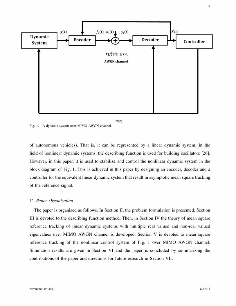
Fig. 1. A dynamic system over MIMO AWGN channel.

of autonomous vehicles). That is, it can be represented by a linear dynamic system. In the

field of nonlinear dynamic systems, the describing function is used for building oscillators [26].

However, in this paper, it is used to stabilize and control the nonlinear dynamic system in the

block diagram of Fig. 1. This is achieved in this paper by designing an encoder, decoder and a

controller for the equivalent linear dynamic system that result in asymptotic mean square tracking

of the reference signal.

C. Paper Organization

The paper is organized as follows. In Section II, the problem formulation is presented. Section

III is devoted to the describing function method. Then, in Section IV the theory of mean square

reference tracking of linear dynamic systems with multiple real valued and non-real valued

eigenvalues over MIMO AWGN channel is developed. Section V is devoted to mean square

reference tracking of the nonlinear control system of Fig. 1 over MIMO AWGN channel.

Simulation results are given in Section VI and the paper is concluded by summarizing the

contributions of the paper and directions for future research in Section VII.


5

II. PROBLEM FORMULATION

Throughout, certain conventions are used: E[·] denotes the expected value, | · | the absolute

value and V ′ the transpose of vector/matrix V . A−1 denotes the inverse of a square matrix A

and N(m,n) the Gaussian distribution with mean m and covariance n. R denotes the set of

real numbers and In the identity matrix with dimension n by n. trac(A) denotes the trace of

a square matrix A, diag{.} denotes the diagonal matrix, [A]ij denotes the i, jth element of the

matrix A and 0 denotes the zero vector/matrix.

This paper is concerned with asymptotic mean square stability and reference tracking of

nonlinear dynamic systems over AWGN communication channel, as is shown in the block

diagram of Fig. 1. The building blocks of Fig. 1 are described below.

Dynamic System: The dynamic system is SISO described by the following nonlinear differ-

ential equation: f(t, x(m), x(m−1), ..., x, u(m), u(m−1), ..., u) = 0

y(t) = x(t)(1)

where x(m)(t) ∈ R is the mth derivative of the system output, u(t) ∈ R is the control input signal,

u(m)(t) ∈ R is the mth derivative of the control input signal and f(t, x(m), x(m−1), ..., x, u(m), u(m−1),

..., u) = 0 is any arbitrary nonlinear differential equation describing the dynamics of the nonlinear

system with the condition that it has periodic outputs in response to sinusoidal inputs.

Communication Channel: Communication channel between system and controller is a MIMO

AWGN channel without interference with n inputs and n outputs. The output of the encoder

(which will be described shortly) is transmitted through the MIMO channel and a white Gaussian

noise vector is added to it (as is shown in Fig. 1), where N(t) =[n1(t) . . . nn(t)

]′i.i.d. ∼

N(0, R) (R = diag{r1, ..., rn}; ri is the variance of the additive noise of the ith input to

output path of the channel) is the MIMO channel noise and ni(t) ∼ N(0, ri) is the additive

noise of the ith input to output path of the MIMO AWGN channel. Also, the MIMO AWGN

channel is subject to the channel input power constraint (Poi, i = 1, 2, ..., n) as follows:

E[f 2i (t)] ≤ Poi, i = 1, 2, ..., n, where fi(t) is the ith element of the encoder output vector

F (t) =[f1(t) . . . fn(t)

]′, that is the input of the channel. Thus, Y (t) = F (t) + N(t),

where Y (t) =[y1(t) . . . yn(t)

]′is the channel output.

Encoder: The encoder is a bandpass filter cascaded with a matrix gain. This bandpass filter

saves only the fundamental frequency of the system output y(t) and omits the other harmonics

which have less information to be sent. For this purpose, a high pass filter with a relatively low


6

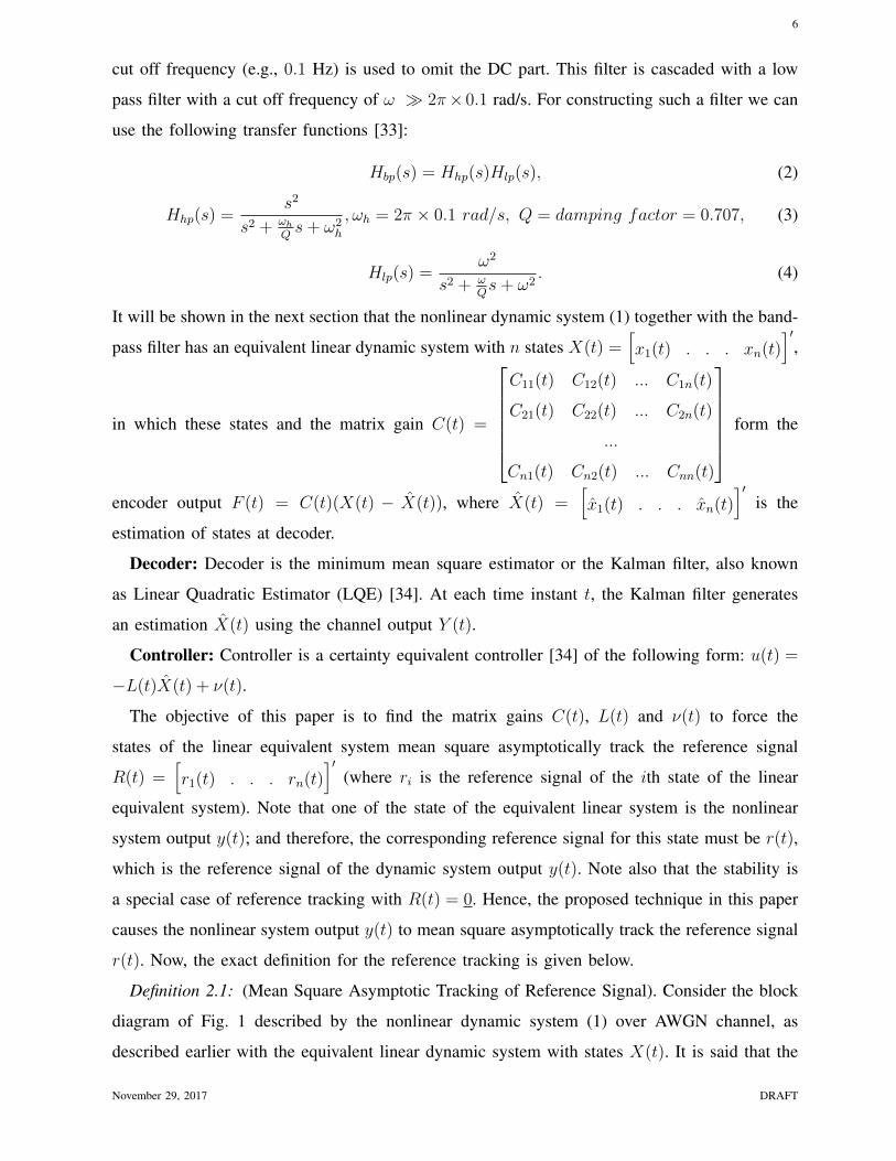
cut off frequency (e.g., 0.1 Hz) is used to omit the DC part. This filter is cascaded with a low

pass filter with a cut off frequency of ω � 2π× 0.1 rad/s. For constructing such a filter we can

use the following transfer functions [33]:

Hbp(s) = Hhp(s)Hlp(s), (2)

Hhp(s) =s2

s2 + ωhQs+ ω2

h

, ωh = 2π × 0.1 rad/s, Q = damping factor = 0.707, (3)

Hlp(s) =ω2

s2 + ωQs+ ω2

. (4)

It will be shown in the next section that the nonlinear dynamic system (1) together with the band-

pass filter has an equivalent linear dynamic system with n states X(t) =[x1(t) . . . xn(t)

]′,

in which these states and the matrix gain C(t) =

C11(t) C12(t) ... C1n(t)

C21(t) C22(t) ... C2n(t)

...

Cn1(t) Cn2(t) ... Cnn(t)

form the

encoder output F (t) = C(t)(X(t) − X(t)), where X(t) =[x1(t) . . . xn(t)

]′is the

estimation of states at decoder.

Decoder: Decoder is the minimum mean square estimator or the Kalman filter, also known

as Linear Quadratic Estimator (LQE) [34]. At each time instant t, the Kalman filter generates

an estimation X(t) using the channel output Y (t).

Controller: Controller is a certainty equivalent controller [34] of the following form: u(t) =

−L(t)X(t) + ν(t).

The objective of this paper is to find the matrix gains C(t), L(t) and ν(t) to force the

states of the linear equivalent system mean square asymptotically track the reference signal

R(t) =[r1(t) . . . rn(t)

]′(where ri is the reference signal of the ith state of the linear

equivalent system). Note that one of the state of the equivalent linear system is the nonlinear

system output y(t); and therefore, the corresponding reference signal for this state must be r(t),

which is the reference signal of the dynamic system output y(t). Note also that the stability is

a special case of reference tracking with R(t) = 0. Hence, the proposed technique in this paper

causes the nonlinear system output y(t) to mean square asymptotically track the reference signal

r(t). Now, the exact definition for the reference tracking is given below.

Definition 2.1: (Mean Square Asymptotic Tracking of Reference Signal). Consider the block

diagram of Fig. 1 described by the nonlinear dynamic system (1) over AWGN channel, as

described earlier with the equivalent linear dynamic system with states X(t). It is said that the


7

system is mean square asymptotically track the reference signal R(t) (and consequently y(t)

tracks r(t)) if there exist an encoder, decoder and a controller such that the following property

holds for all choices of the initial conditions in spite of the noise and the channel input power

constraint.

limt→∞

E[(xi(t)− ri(t))2] = 0,

subject to E[f 2i (t)] ≤ Poi, ∀i. (5)

III. IMPLEMENTATION OF DESCRIBING FUNCTION METHOD

In this section, we use the idea of describing function to obtain the equivalent linear dynamic

system for the nonlinear dynamic system (1). Then, in the next section we propose an encoder,

decoder and a controller for mean square asymptotic tracking of the equivalent linear dynamic

system, as defined in this section.

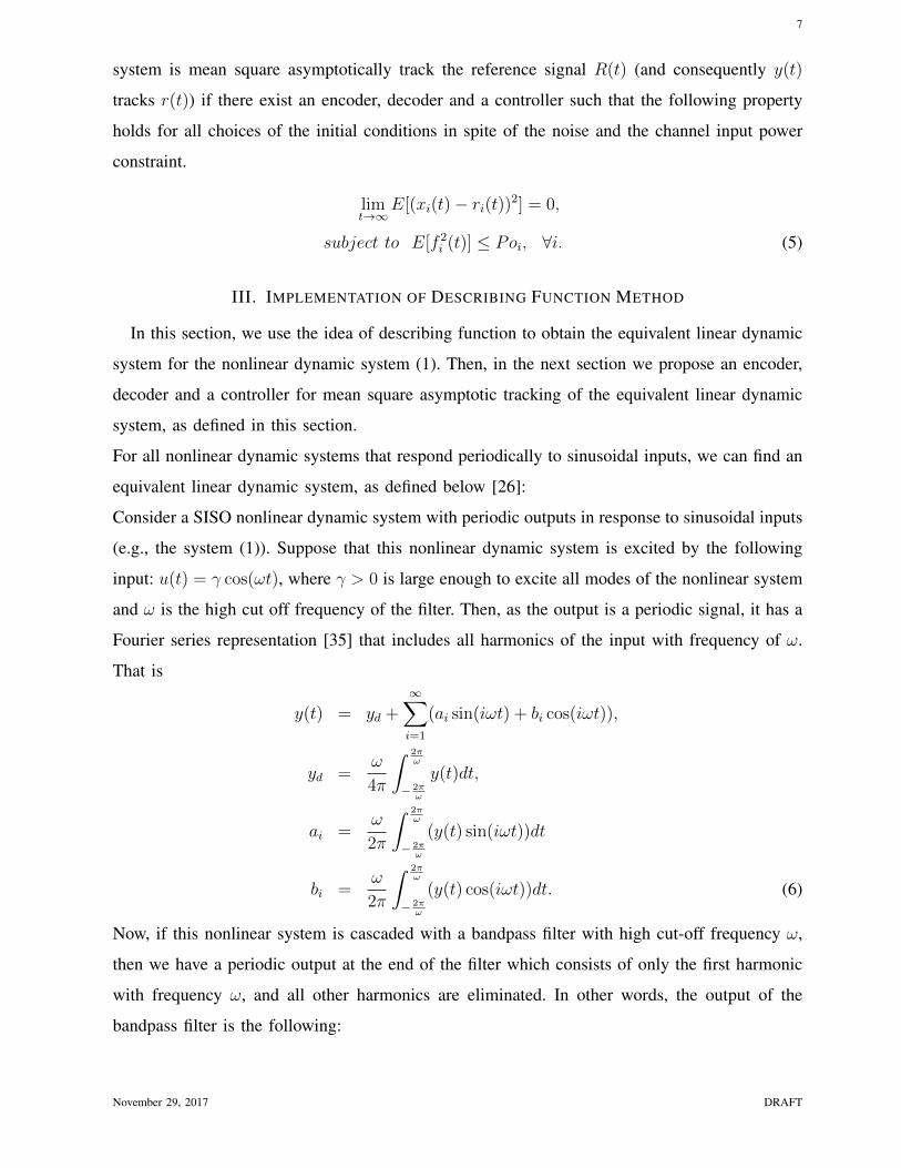
For all nonlinear dynamic systems that respond periodically to sinusoidal inputs, we can find an

equivalent linear dynamic system, as defined below [26]:

Consider a SISO nonlinear dynamic system with periodic outputs in response to sinusoidal inputs

(e.g., the system (1)). Suppose that this nonlinear dynamic system is excited by the following

input: u(t) = γ cos(ωt), where γ > 0 is large enough to excite all modes of the nonlinear system

and ω is the high cut off frequency of the filter. Then, as the output is a periodic signal, it has a

Fourier series representation [35] that includes all harmonics of the input with frequency of ω.

That is

y(t) = yd +∞∑i=1

(ai sin(iωt) + bi cos(iωt)),

yd =ω

4π

∫ 2πω

− 2πω

y(t)dt,

ai =ω

2π

∫ 2πω

− 2πω

(y(t) sin(iωt))dt

bi =ω

2π

∫ 2πω

− 2πω

(y(t) cos(iωt))dt. (6)

Now, if this nonlinear system is cascaded with a bandpass filter with high cut-off frequency ω,

then we have a periodic output at the end of the filter which consists of only the first harmonic

with frequency ω, and all other harmonics are eliminated. In other words, the output of the

bandpass filter is the following:


8

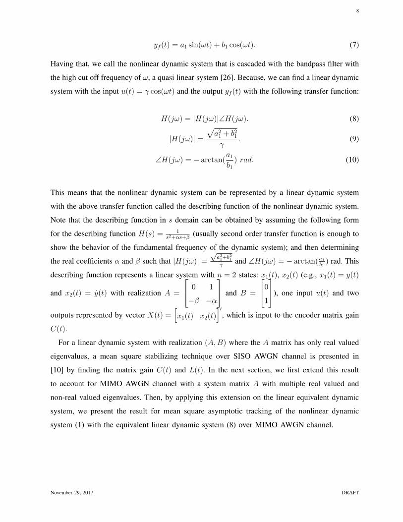
yf (t) = a1 sin(ωt) + b1 cos(ωt). (7)

Having that, we call the nonlinear dynamic system that is cascaded with the bandpass filter with

the high cut off frequency of ω, a quasi linear system [26]. Because, we can find a linear dynamic

system with the input u(t) = γ cos(ωt) and the output yf (t) with the following transfer function:

H(jω) = |H(jω)|∠H(jω). (8)

|H(jω)| =√a21 + b21γ

. (9)

∠H(jω) = − arctan(a1b1

) rad. (10)

This means that the nonlinear dynamic system can be represented by a linear dynamic system

with the above transfer function called the describing function of the nonlinear dynamic system.

Note that the describing function in s domain can be obtained by assuming the following form

for the describing function H(s) = 1s2+αs+β

(usually second order transfer function is enough to

show the behavior of the fundamental frequency of the dynamic system); and then determining

the real coefficients α and β such that |H(jω)| =√a21+b

21

γand ∠H(jω) = − arctan(a1

b1) rad. This

describing function represents a linear system with n = 2 states: x1(t), x2(t) (e.g., x1(t) = y(t)

and x2(t) = y(t) with realization A =

0 1

−β −α

and B =

0

1

), one input u(t) and two

outputs represented by vector X(t) =[x1(t) x2(t)

]′, which is input to the encoder matrix gain

C(t).

For a linear dynamic system with realization (A,B) where the A matrix has only real valued

eigenvalues, a mean square stabilizing technique over SISO AWGN channel is presented in

[10] by finding the matrix gain C(t) and L(t). In the next section, we first extend this result

to account for MIMO AWGN channel with a system matrix A with multiple real valued and

non-real valued eigenvalues. Then, by applying this extension on the linear equivalent dynamic

system, we present the result for mean square asymptotic tracking of the nonlinear dynamic

system (1) with the equivalent linear dynamic system (8) over MIMO AWGN channel.


9

IV. LINEAR SYSTEM WITH MULTIPLE REAL VALUED AND NON-REAL VALUED

EIGENVALUES

Now, we extend the result of [10] to account for reference tracking and hence stability of linear

continuous time dynamic systems with multiple real valued and non-real valued eigenvalues over

MIMO AWGN channel.

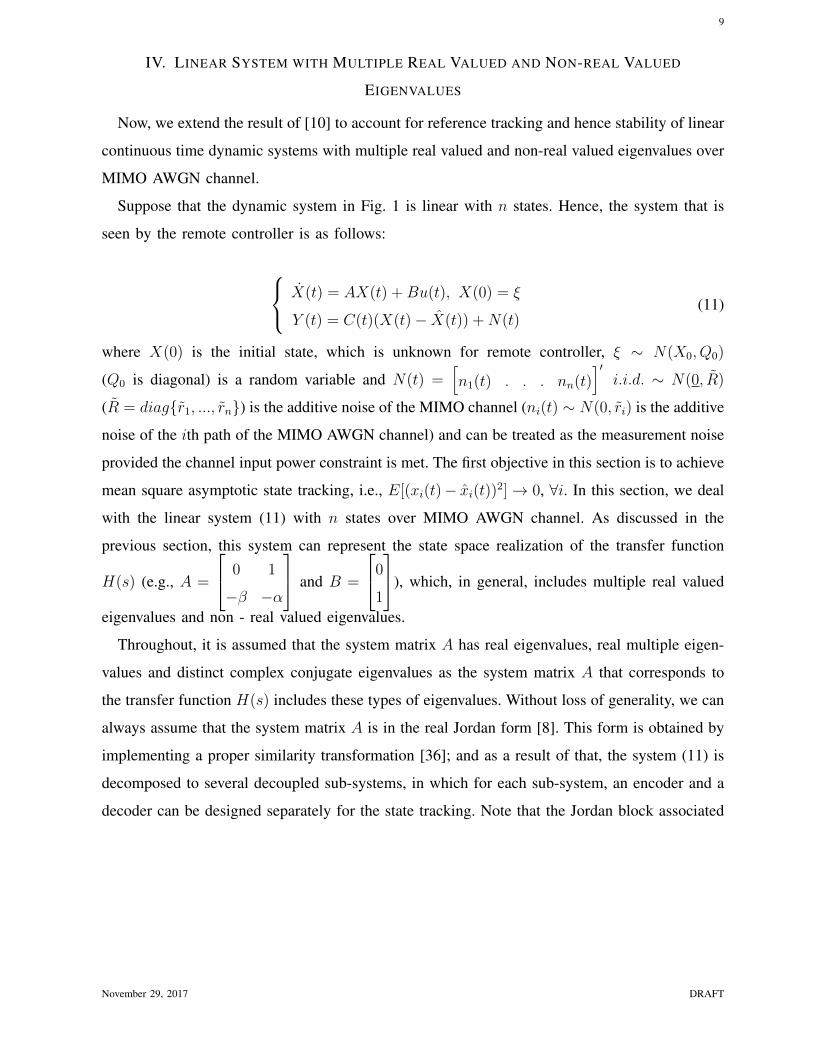
Suppose that the dynamic system in Fig. 1 is linear with n states. Hence, the system that is

seen by the remote controller is as follows:

X(t) = AX(t) +Bu(t), X(0) = ξ

Y (t) = C(t)(X(t)− X(t)) +N(t)(11)

where X(0) is the initial state, which is unknown for remote controller, ξ ∼ N(X0, Q0)

(Q0 is diagonal) is a random variable and N(t) =[n1(t) . . . nn(t)

]′i.i.d. ∼ N(0, R)

(R = diag{r1, ..., rn}) is the additive noise of the MIMO channel (ni(t) ∼ N(0, ri) is the additive

noise of the ith path of the MIMO AWGN channel) and can be treated as the measurement noise

provided the channel input power constraint is met. The first objective in this section is to achieve

mean square asymptotic state tracking, i.e., E[(xi(t)− xi(t))2]→ 0, ∀i. In this section, we deal

with the linear system (11) with n states over MIMO AWGN channel. As discussed in the

previous section, this system can represent the state space realization of the transfer function

H(s) (e.g., A =

0 1

−β −α

and B =

0

1

), which, in general, includes multiple real valued

eigenvalues and non - real valued eigenvalues.

Throughout, it is assumed that the system matrix A has real eigenvalues, real multiple eigen-

values and distinct complex conjugate eigenvalues as the system matrix A that corresponds to

the transfer function H(s) includes these types of eigenvalues. Without loss of generality, we can

always assume that the system matrix A is in the real Jordan form [8]. This form is obtained by

implementing a proper similarity transformation [36]; and as a result of that, the system (11) is

decomposed to several decoupled sub-systems, in which for each sub-system, an encoder and a

decoder can be designed separately for the state tracking. Note that the Jordan block associated


10

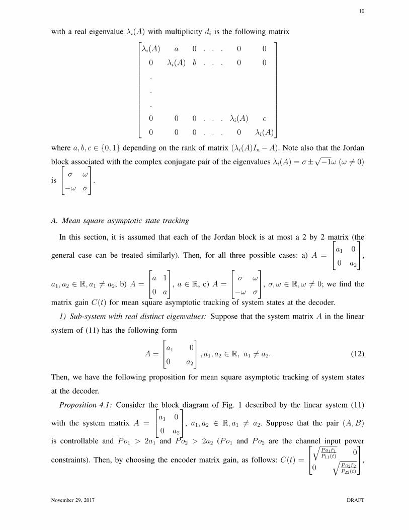
with a real eigenvalue λi(A) with multiplicity di is the following matrix

λi(A) a 0 . . . 0 0

0 λi(A) b . . . 0 0

.

.

.

0 0 0 . . . λi(A) c

0 0 0 . . . 0 λi(A)

where a, b, c ∈ {0, 1} depending on the rank of matrix (λi(A)In−A). Note also that the Jordan

block associated with the complex conjugate pair of the eigenvalues λi(A) = σ±√−1ω (ω 6= 0)

is

σ ω

−ω σ

.

A. Mean square asymptotic state tracking

In this section, it is assumed that each of the Jordan block is at most a 2 by 2 matrix (the

general case can be treated similarly). Then, for all three possible cases: a) A =

a1 0

0 a2

,

a1, a2 ∈ R, a1 6= a2, b) A =

a 1

0 a

, a ∈ R, c) A =

σ ω

−ω σ

, σ, ω ∈ R, ω 6= 0; we find the

matrix gain C(t) for mean square asymptotic tracking of system states at the decoder.

1) Sub-system with real distinct eigenvalues: Suppose that the system matrix A in the linear

system of (11) has the following form

A =

a1 0

0 a2

, a1, a2 ∈ R, a1 6= a2. (12)

Then, we have the following proposition for mean square asymptotic tracking of system states

at the decoder.

Proposition 4.1: Consider the block diagram of Fig. 1 described by the linear system (11)

with the system matrix A =

a1 0

0 a2

, a1, a2 ∈ R, a1 6= a2. Suppose that the pair (A,B)

is controllable and Po1 > 2a1 and Po2 > 2a2 (Po1 and Po2 are the channel input power

constraints). Then, by choosing the encoder matrix gain, as follows: C(t) =

√Po1r1P11(t)

0

0√

Po2r2P22(t)

,


11

and a decoder with the following description (which is the Kalman filter [34])

˙X(t) = AX(t) +Bu(t) +K(t)Y (t), X(0) = X0,

K(t) = P (t)C ′(t)R−1, R = diag{r1, r2}

P (t) = A′P (t)+P (t)A−P (t)C ′(t)R−1C(t)P (t), P (0) = Q0, P (t) = P ′(t) =

P11(t) P12(t)

P12(t) P22(t)

≥ 0

we have mean square asymptotic tracking of system states at the decoder.

Proof: The encoder matrix gain has the following general form C(t) =

C11(t) C12(t)

C21(t) C22(t)

;

and subsequently, the decoder can be extracted as follows (for the simplicity of presentation the

dependency to the time index t is dropped):

P11 = 2a1P11 − (2P11P12C11C12r−11 + 2P11P12C21C22r

−12 + P 2

11C211r−11 + P 2

12C212r−11

+P 211C

221r−12 + P 2

12C222r−12 )

˙P22 = 2a2P22 − (2P22P12C22C21r−12 + 2P22P12C21C11r

−11 + P 2

22C222r−12 + P 2

12C221r−12

+P 222C

212r−11 + P 2

12C211r−11 )

˙P12 = a1P12 + a2P12 − r−11 (P11P12C211 + P 2

12C11C12 + P11P22C11C12 + P12P22C212)

−r−12 (P11P12C221 + P 2

12C22C21 + P11P22C22C21 + P12P22C222)

(13)

Now, by substituting C11(t) =√

Po1r1P11(t)

, C22(t) =√

Po2r2P22(t)

and C12(t) = C21(t) = 0 in the above

expressions, we have P12(t) = 0 and P12(t) = P12(0) = [Q0]12 = 0. Thus, we have

P11(t) = (2a1 − Po1)P11(t)⇒ P11(t) = e−(Po1−2a1)tP11(0). (14)

P22(t) = (2a2 − Po2)P22(t)⇒ P22(t) = e−(Po2−2a2)tP22(0). (15)

In summary, by the above selection, we have

P (t) =

e−(Po1−2a1)tP11(0) 0

0 e−(Po2−2a2)tP22(0)

(16)

and the following description for the decoder:

˙X(t) = AX(t) +Bu(t) +K(t)Y (t), K(t) = P (t)C

′(t)R−1, X(0) = X0. (17)

Now, as we assumed that Po1 > 2a1 and Po2 > 2a2, we have limt→∞E[(x1(t) − x1(t))2] =

limt→∞ P11(t) = limt→∞ e−(Po1−2a1)tP11(0) = 0. Similarly, we have limt→∞E[(x2(t)−x2(t))2] =

limt→∞ P22(t) = 0. Hence, P (t)→ P =

0 0

0 0

. This completes the proof.


12

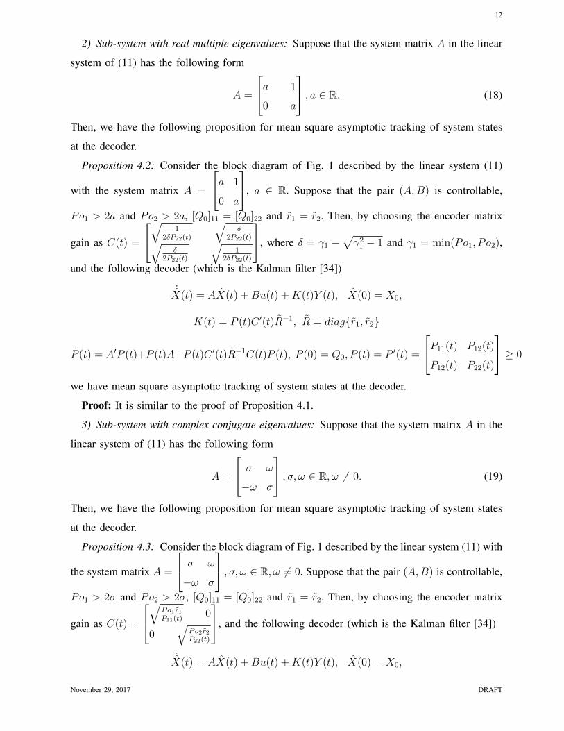
2) Sub-system with real multiple eigenvalues: Suppose that the system matrix A in the linear

system of (11) has the following form

A =

a 1

0 a

, a ∈ R. (18)


at the decoder.

Proposition 4.2: Consider the block diagram of Fig. 1 described by the linear system (11)

with the system matrix A =

a 1

0 a

, a ∈ R. Suppose that the pair (A,B) is controllable,

Po1 > 2a and Po2 > 2a, [Q0]11 = [Q0]22 and r1 = r2. Then, by choosing the encoder matrix

gain as C(t) =

√ 12δP22(t)

√δ

2P22(t)√δ

2P22(t)

√1

2δP22(t)

, where δ = γ1 −√γ21 − 1 and γ1 = min(Po1, Po2),

and the following decoder (which is the Kalman filter [34])

˙X(t) = AX(t) +Bu(t) +K(t)Y (t), X(0) = X0,

K(t) = P (t)C ′(t)R−1, R = diag{r1, r2}


P11(t) P12(t)

P12(t) P22(t)

≥ 0


Proof: It is similar to the proof of Proposition 4.1.

3) Sub-system with complex conjugate eigenvalues: Suppose that the system matrix A in the

linear system of (11) has the following form

A =

σ ω

−ω σ

, σ, ω ∈ R, ω 6= 0. (19)


at the decoder.

Proposition 4.3: Consider the block diagram of Fig. 1 described by the linear system (11) with

the system matrix A =

σ ω

−ω σ

, σ, ω ∈ R, ω 6= 0. Suppose that the pair (A,B) is controllable,

Po1 > 2σ and Po2 > 2σ, [Q0]11 = [Q0]22 and r1 = r2. Then, by choosing the encoder matrix

gain as C(t) =

√Po1r1P11(t)

0

0√

Po2r2P22(t)

, and the following decoder (which is the Kalman filter [34])

˙X(t) = AX(t) +Bu(t) +K(t)Y (t), X(0) = X0,


13

K(t) = P (t)C ′(t)R−1, R = diag{r1, r2}


P11(t) P12(t)

P12(t) P22(t)

≥ 0


Proof: It is similar to the proof of Proposition 4.1.

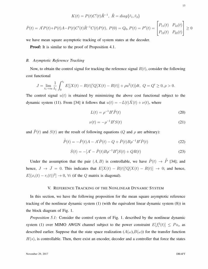
B. Asymptotic Reference Tracking

Now, to obtain the control signal for tracking the reference signal R(t), consider the following

cost functional

J = limt1→∞

1

t1

∫ t1

0

E[[X(t)−R(t)]′Q[X(t)−R(t)] + ρu2(t)]dt, Q = Q′ ≥ 0, ρ > 0.

The control signal u(t) is obtained by minimizing the above cost functional subject to the

dynamic system (11). From [34] it follows that u(t) = −L(t)X(t) + ν(t), where

L(t) = ρ−1B′P (t) (20)

ν(t) = −ρ−1B′S(t) (21)

and P (t) and S(t) are the result of following equations (Q and ρ are arbitrary):

˙P (t) = −P (t)A− A′P (t)−Q+ P (t)Bρ−1B′P (t) (22)

S(t) = −[A′ − P (t)Bρ−1B′]S(t) +QR(t) (23)

Under the assumption that the pair (A,B) is controllable, we have P (t) → ¯P [34]; and

hence, J → J = 0. This indicates that E[X(t) − R(t)]′Q[X(t) − R(t)] → 0; and hence,

E[(xi(t)− ri(t))2]→ 0, ∀i (if the Q matrix is diagonal).

V. REFERENCE TRACKING OF THE NONLINEAR DYNAMIC SYSTEM

In this section, we have the following proposition for the mean square asymptotic reference

tracking of the nonlinear dynamic system (1) (with the equivalent linear dynamic system (8)) in

the block diagram of Fig. 1.

Proposition 5.1: Consider the control system of Fig. 1. described by the nonlinear dynamic

system (1) over MIMO AWGN channel subject to the power constraint E[f 2i (t)] ≤ Poi, as

described earlier. Suppose that the state space realization (A(ω),B(ω)) for the transfer function

H(s), is controllable. Then, there exist an encoder, decoder and a controller that force the states


14

𝒚(𝒕) 𝑭(𝒕) 𝑵(𝒕) ��(𝒕)

𝒖(𝒕)

Nonlinear

Dynamic

System

Encoder Decoder

Controller

𝑹(𝒕)

𝒌

𝒔

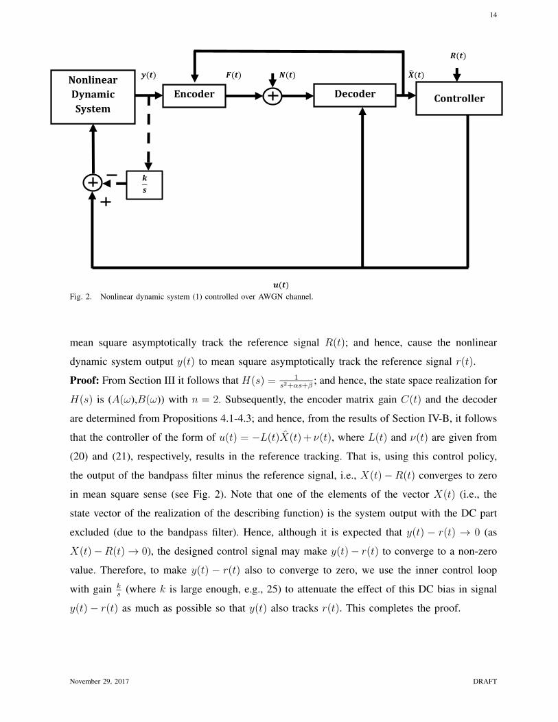
Fig. 2. Nonlinear dynamic system (1) controlled over AWGN channel.

mean square asymptotically track the reference signal R(t); and hence, cause the nonlinear

dynamic system output y(t) to mean square asymptotically track the reference signal r(t).

Proof: From Section III it follows that H(s) = 1s2+αs+β

; and hence, the state space realization for

H(s) is (A(ω),B(ω)) with n = 2. Subsequently, the encoder matrix gain C(t) and the decoder

are determined from Propositions 4.1-4.3; and hence, from the results of Section IV-B, it follows

that the controller of the form of u(t) = −L(t)X(t) + ν(t), where L(t) and ν(t) are given from

(20) and (21), respectively, results in the reference tracking. That is, using this control policy,

the output of the bandpass filter minus the reference signal, i.e., X(t)−R(t) converges to zero

in mean square sense (see Fig. 2). Note that one of the elements of the vector X(t) (i.e., the

state vector of the realization of the describing function) is the system output with the DC part

excluded (due to the bandpass filter). Hence, although it is expected that y(t) − r(t) → 0 (as

X(t)−R(t)→ 0), the designed control signal may make y(t)− r(t) to converge to a non-zero

value. Therefore, to make y(t) − r(t) also to converge to zero, we use the inner control loop

with gain ks

(where k is large enough, e.g., 25) to attenuate the effect of this DC bias in signal

y(t)− r(t) as much as possible so that y(t) also tracks r(t). This completes the proof.


15

VI. SIMULATIONS RESULTS

In this section, for the purpose of illustration, we apply the proposed encoder, decoder and

controller to a DC motor with saturation element, that is used in our laboratory to protect the DC

motor from high input voltage as is shown in Fig. 3. Systems with actuator saturation and hard

constraints are important class of dynamic systems and have been considered in the literature

(e.g., [37]-[39]). The DC motor considered in this paper has the following description x(t) = −0.96x(t) + 178.85u(t)

y(t) = x(t),(24)

where u(t) is the output of the saturation element. The saturation element saturates the control

signal u(t) between -10 and +10 volts. That is,

u(t) =

10, u(t) ≥ 10

u(t), |u(t)| < 10

−10, u(t) ≤ −10

(25)

For the remote controller the initial condition is unknown and has the following description

x(0) ∼ N(0, 1). The system must track the reference signal r(t). The MIMO AWGN channel has

the following specification: N(t) i.i.d. ∼ N(0, diag{1, 1}), with the following power constraints

Po1 = 2 and Po2 = 2 to satisfy the requirements of Propositions 4.1-4.3.

The linear dynamic system (24) can be treated as a low pass filter, which is cascaded with

the nonlinear saturation block (see Fig. 3). Hence, this block together with the linear dynamic

system (24) has a quasi linear representation described by the describing function. To obtain this

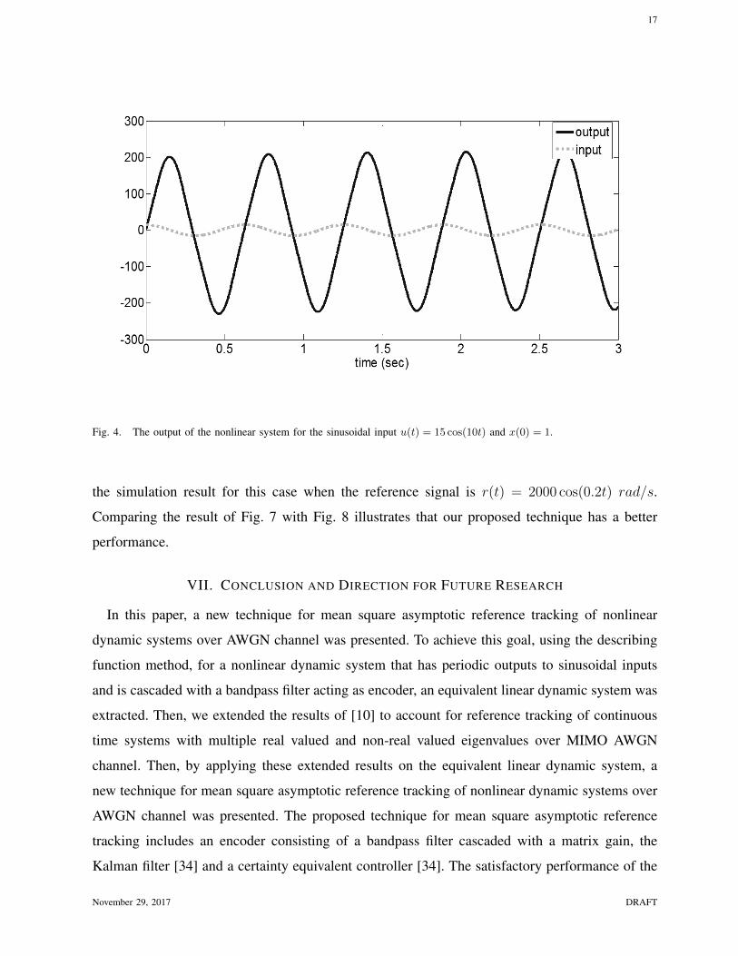
describing function for a given ω, e.g., ω = 10, we apply the following sinusoidal input to the

system:

u(t) = 15 cos(10t). (26)

The steady state output of this excitation signal is:

y(t) = x(t) = 208.5 cos(10t+ 1.67) rad/s, (27)

which is shown in Fig. 4. From this input and output, the describing function is H(s) =

1s2+0.00716s+99.99

; and therefore, the equivalent linear dynamic system that is seen by the remote


16

𝒚(𝒕) 𝑭(𝒕) 𝑵(𝒕) ��(𝒕)

𝒖(𝒕)

DC

Motor Encode

r

Decoder

Controller

𝑹(𝒕)

Integrator

Saturation

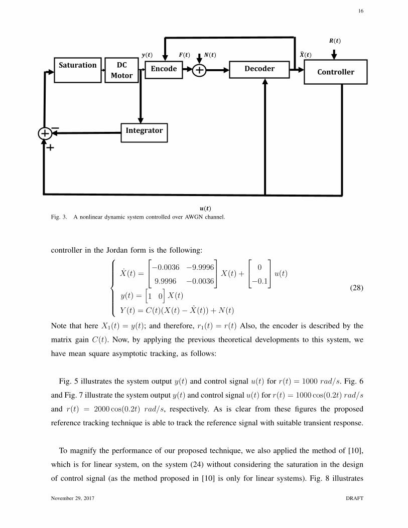
Fig. 3. A nonlinear dynamic system controlled over AWGN channel.

controller in the Jordan form is the following:X(t) =

−0.0036 −9.9996

9.9996 −0.0036

X(t) +

0

−0.1

u(t)

y(t) =[1 0

]X(t)

Y (t) = C(t)(X(t)− X(t)) +N(t)

(28)

Note that here X1(t) = y(t); and therefore, r1(t) = r(t) Also, the encoder is described by the

matrix gain C(t). Now, by applying the previous theoretical developments to this system, we

have mean square asymptotic tracking, as follows:

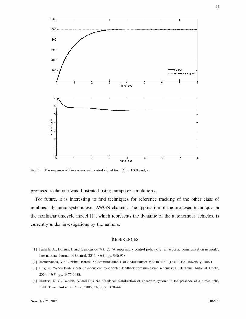
Fig. 5 illustrates the system output y(t) and control signal u(t) for r(t) = 1000 rad/s. Fig. 6

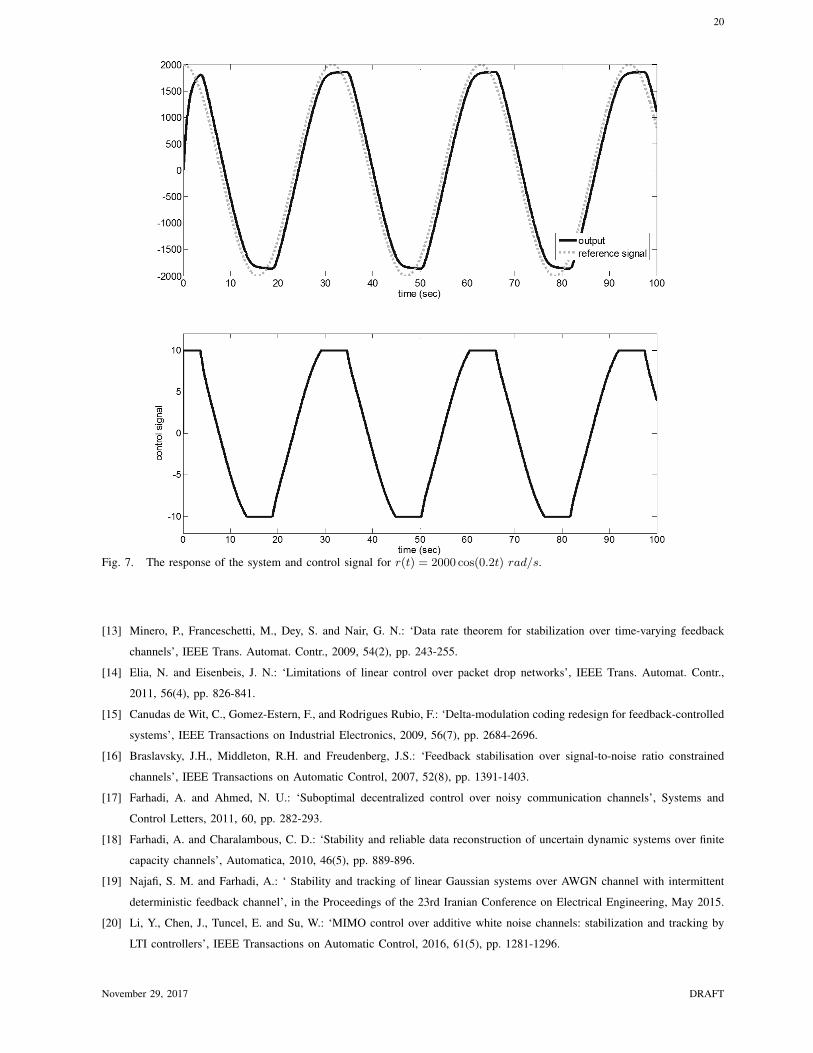
and Fig. 7 illustrate the system output y(t) and control signal u(t) for r(t) = 1000 cos(0.2t) rad/s

and r(t) = 2000 cos(0.2t) rad/s, respectively. As is clear from these figures the proposed

reference tracking technique is able to track the reference signal with suitable transient response.

To magnify the performance of our proposed technique, we also applied the method of [10],

which is for linear system, on the system (24) without considering the saturation in the design

of control signal (as the method proposed in [10] is only for linear systems). Fig. 8 illustrates


17

Fig. 4. The output of the nonlinear system for the sinusoidal input u(t) = 15 cos(10t) and x(0) = 1.

the simulation result for this case when the reference signal is r(t) = 2000 cos(0.2t) rad/s.

Comparing the result of Fig. 7 with Fig. 8 illustrates that our proposed technique has a better

performance.

VII. CONCLUSION AND DIRECTION FOR FUTURE RESEARCH

In this paper, a new technique for mean square asymptotic reference tracking of nonlinear

dynamic systems over AWGN channel was presented. To achieve this goal, using the describing

function method, for a nonlinear dynamic system that has periodic outputs to sinusoidal inputs

and is cascaded with a bandpass filter acting as encoder, an equivalent linear dynamic system was

extracted. Then, we extended the results of [10] to account for reference tracking of continuous

time systems with multiple real valued and non-real valued eigenvalues over MIMO AWGN

channel. Then, by applying these extended results on the equivalent linear dynamic system, a

new technique for mean square asymptotic reference tracking of nonlinear dynamic systems over

AWGN channel was presented. The proposed technique for mean square asymptotic reference

tracking includes an encoder consisting of a bandpass filter cascaded with a matrix gain, the

Kalman filter [34] and a certainty equivalent controller [34]. The satisfactory performance of the


18

Fig. 5. The response of the system and control signal for r(t) = 1000 rad/s.

proposed technique was illustrated using computer simulations.

For future, it is interesting to find techniques for reference tracking of the other class of

nonlinear dynamic systems over AWGN channel. The application of the proposed technique on

the nonlinear unicycle model [1], which represents the dynamic of the autonomous vehicles, is

currently under investigations by the authors.

REFERENCES

[1] Farhadi, A., Domun, J. and Canudas de Wit, C.: ‘A supervisory control policy over an acoustic communication network’,

International Journal of Control, 2015, 88(5), pp. 946-958.

[2] Memarzadeh, M.:‘ Optimal Borehole Communication Using Multicarrier Modulation’, (Diss. Rice University, 2007).

[3] Elia, N.: ‘When Bode meets Shannon: control-oriented feedback communication schemes’, IEEE Trans. Automat. Contr.,

2004, 49(9), pp. 1477-1488.

[4] Martins, N. C., Dahleh, A. and Elia N.: ‘Feedback stabilization of uncertain systems in the presence of a direct link’,

IEEE Trans. Automat. Contr., 2006, 51(3), pp. 438-447.


19

Fig. 6. The response of the system and control signal for r(t) = 1000 cos(0.2t) rad/s.

[5] Minero, P., Coviello, L. and Franceschetti, M.: ‘Stabilization over Markov feedback channels: the general case’, IEEE

Trans. Automat. Contr., 2013, 58(2), pp. 349-362.

[6] Nair, G. N., Evans, R. J., Mareels, I. M. Y. and Moran, W.: ‘Topological feedback entropy and nonlinear stabilization’,

IEEE Trans. Automat. Contr., 2004, 49(9), pp. 1585-1597.

[7] Nair, G. N. and Evans, R. J.: ‘Stabilizability of stochastic linear systems with finite feedback data rates’, SIAM J. Control

Optimization, 2004, 43(3), pp. 413-436.

[8] Tatikonda, S. and Mitter, S. :‘Control under communication constraints’, IEEE Transactions on Automatic Control, 2004,

49(7), pp. 1056-1068.

[9] Charalambous, C. D. and Farhadi, A.: ‘LQG optimality and separation principle for general discrete time partially observed

stochastic systems over finite capacity communication channels’, Automatica, 2008, 44(12), pp. 3181-3188.

[10] Charalambous, C. D., Farhadi, A. and Denic, S. Z.: ‘Control of continuous-time linear Gaussian systems over additive

Gaussian wireless fading channels: a separation principle’, IEEE Trans. Automat. Contr., 2008, 53(4), pp. 1013-1019.

[11] Farhadi, A.: ‘Stability of linear dynamic systems over the packet erasure channel: a co-design approach’, International

Journal of Control, 2015, 88(12), pp. 2488-2498.

[12] Farhadi, A.: ‘Feedback channel in linear noiseless dynamic systems controlled over the packet erasure network’,

International Journal of Control, 2015, 88(8), pp. 1490-1503.


20

Fig. 7. The response of the system and control signal for r(t) = 2000 cos(0.2t) rad/s.

[13] Minero, P., Franceschetti, M., Dey, S. and Nair, G. N.: ‘Data rate theorem for stabilization over time-varying feedback

channels’, IEEE Trans. Automat. Contr., 2009, 54(2), pp. 243-255.

[14] Elia, N. and Eisenbeis, J. N.: ‘Limitations of linear control over packet drop networks’, IEEE Trans. Automat. Contr.,

2011, 56(4), pp. 826-841.

[15] Canudas de Wit, C., Gomez-Estern, F., and Rodrigues Rubio, F.: ‘Delta-modulation coding redesign for feedback-controlled

systems’, IEEE Transactions on Industrial Electronics, 2009, 56(7), pp. 2684-2696.

[16] Braslavsky, J.H., Middleton, R.H. and Freudenberg, J.S.: ‘Feedback stabilisation over signal-to-noise ratio constrained

channels’, IEEE Transactions on Automatic Control, 2007, 52(8), pp. 1391-1403.

[17] Farhadi, A. and Ahmed, N. U.: ‘Suboptimal decentralized control over noisy communication channels’, Systems and

Control Letters, 2011, 60, pp. 282-293.

[18] Farhadi, A. and Charalambous, C. D.: ‘Stability and reliable data reconstruction of uncertain dynamic systems over finite

capacity channels’, Automatica, 2010, 46(5), pp. 889-896.

[19] Najafi, S. M. and Farhadi, A.: ‘ Stability and tracking of linear Gaussian systems over AWGN channel with intermittent

deterministic feedback channel’, in the Proceedings of the 23rd Iranian Conference on Electrical Engineering, May 2015.

[20] Li, Y., Chen, J., Tuncel, E. and Su, W.: ‘MIMO control over additive white noise channels: stabilization and tracking by

LTI controllers’, IEEE Transactions on Automatic Control, 2016, 61(5), pp. 1281-1296.


21

Fig. 8. The response of the system and control signal of the linear method of [10] for r(t) = 2000 cos(0.2t) rad/s.

[21] Wu, J. and Chen, T.:‘ Design of networked control systems with packet dropouts’, IEEE Transactions on Automatic Control,

2007, 52(7), 1314 - 1319.

[22] Cover, T. A. and Thomas, J. A.:‘ Elements of Information Theory’, (John Wiley and Sons, 1991).

[23] Judd, K. L.: ‘Numerical Methods in Economics’, (Cambridge, MA: MIT Press, 1998).

[24] Mees, A. I.: ‘Dynamics of Feedback Systems’, (New York: Wiley, 1981).

[25] Gilmore, R. J. and Steer, M. B.: ‘Nonlinear circuit analysis using the method of harmonic balance A review of the art.

Part I. Introductory concepts’, Int. J. Microw. Mill.-Wave Comput.-Aided Eng., 1991, 1, pp. 22 27.

[26] Slotine, J. J. and Li, W.: ‘Applied Nonlinear Control’, (Prentice-Hall, 1991).

[27] Jing, Xi. and Lang, Zi.: ‘Frequency Domain Analysis and Design of Nonlinear Systems Based on Volterra Series Expansion

- A Parametric Characteristic Approach’, (Springer International Publishing Switzerland, 2015).

[28] Rugh, W. J.: ‘Nonlinear System Theory: The Volterra/Wiener Approach’, (Baltimore, MD: The Johns Hopkins Univ. Press,

1981).

[29] Worden, K. and Tomlinson, G. R.: ‘Nonlinearity in Structural Dynamics: Detection, Identification and Modeling’, (Bristol,

U.K.: Institute of Physics, 2001).

[30] George, D. A.: ‘Continuous Nonlinear Systems’, (MIT Research Lab. Electronics, Cambridge, MA, Tech. Rep. 355, 1959).

[31] Xiao, Z. and Jing, X.: ‘Frequency-domain analysis and design of linear feedback of nonlinear systems and applications in


22

vehicle suspensions’, IEEE/ASME Transactions on Mechatronics, 2016, 21(1), pp. 506-517.

[32] Jing, X.: ‘Nonlinear characteristic output spectrum for nonlinear analysis and design’, IEEE/ASME Transactions on

Mechatronics, 2014, 19(1), pp. 171-183.

[33] Shenoi, B. A.:‘ Introduction to Digital Signal Processing and Filter Design’, (John Wiley and Sons, 2006).

[34] Kwakernaak, H. and Sivan, P.: ‘Linear Optimal Control Systems’, (Wiley-Interscience, 1972).

[35] Rudin, W.:‘ Principle of Mathematical Analysis’, (New York: McGraw - Hill, Inc., 1976).

[36] Strang, G.:‘ Introduction to Linear Algebra’, (Wellesley - Cambridge Press, 2016).

[37] Pan, H., Sun, W., Gao, H. and Jing, X.: ‘Disturbance observer-based adaptive tracking control with actuator saturation and

its application’, IEEE Transactions on Automation Science and Engineering, 2016, 13(2), pp. 868-875.

[38] Pan, H., Sun, W., Gao, H. and Yu, J.: ‘Finite-time stabilization for vehicle active suspension systems with hard constraints’,

IEEE Transactions on Intelligent Transportation Systems, 2015, 16(5), pp. 2663-2672.

[39] Sun, W., Pan, H. and Gao, H.: ‘Filter-based adaptive vibration control for active vehicle suspensions with electrohydraulic

actuators’, IEEE Transactions on Vehicular Technology, 2016, 65(6), pp. 4619-4626.

Biography

Ali Parsa is currently Ph.D. student in the Department of Electrical Engineering at Sharif

University of Technology. His research is concerned with control over communication. He

received his B.Sc. and M.Sc. degrees in Electrical Engineering from the University of Tehran,

Iran.

Alireza Farhadi received Ph.D. degree in Electrical Engineering from the University of Ottawa,

Ontario, Canada in 2007. After receiving Ph.D. degree, Dr. Farhadi worked as Postdoctoral

Fellow in the Department of Electrical Engineering of the University of Ottawa (2008-2009) and

the French National Institute for Research in Computer Science and Control (INRIA), Grenoble,

France (2010-2011). He then worked as Research Fellow (academic level B) in the Department

of Electrical Engineering of the University of Melbourne, Australia (2011-2013). In September

2013, he joined the Department of Electrical Engineering of the Sharif University of Technology

as Assistant Professor. Dr. Farhadi’s areas of expertise are networked control systems, distributed

optimal control, stochastic and nonlinear controls, automated irrigation networks and Internet of

Things (IoT).


reference tracking of nonlinear dynamic systems over...

Documents