reduction of sampling inspection using variables …...reduction of sampling inspection using...

Reduction of Sampling Inspection Using Variables Data in the Presence of

Batch-to-Batch Variability

David Trindade, Ph.D.

[email protected]

JMP Discovery Summit, Carey, NC September 2014

Attributes Sampling

In attributes sampling, a specified sample size is randomly

selected from a batch, and the CTQs (Critical To Quality)

parameters are measured and compared to specification

limits. Samples not meeting these limits are counted as

defective.

Incoming Quality Control (IQC) had been inspecting batches

using attributes sampling plans, measuring many CTQs on

typically n = 80 parts. The batch would be accepted for c = 0

defectives and rejected for c = 1 or more defectives.

This sampling plan corresponds to acceptable quality levels

(AQL’s) and rejectable quality levels (RQL’s) of the

proportion defective shown on the next slide.

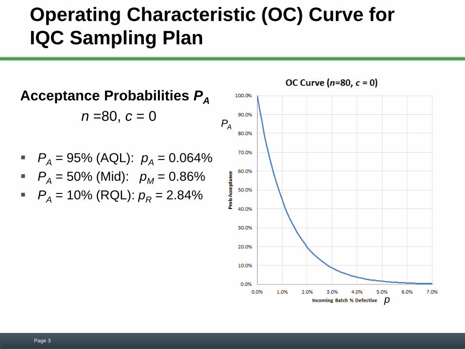
Operating Characteristic (OC) Curve for

IQC Sampling Plan

Acceptance Probabilities PA

n =80, c = 0

PA = 95% (AQL): pA = 0.064%

PA = 50% (Mid): pM = 0.86%

PA = 10% (RQL): pR = 2.84%

p

PA

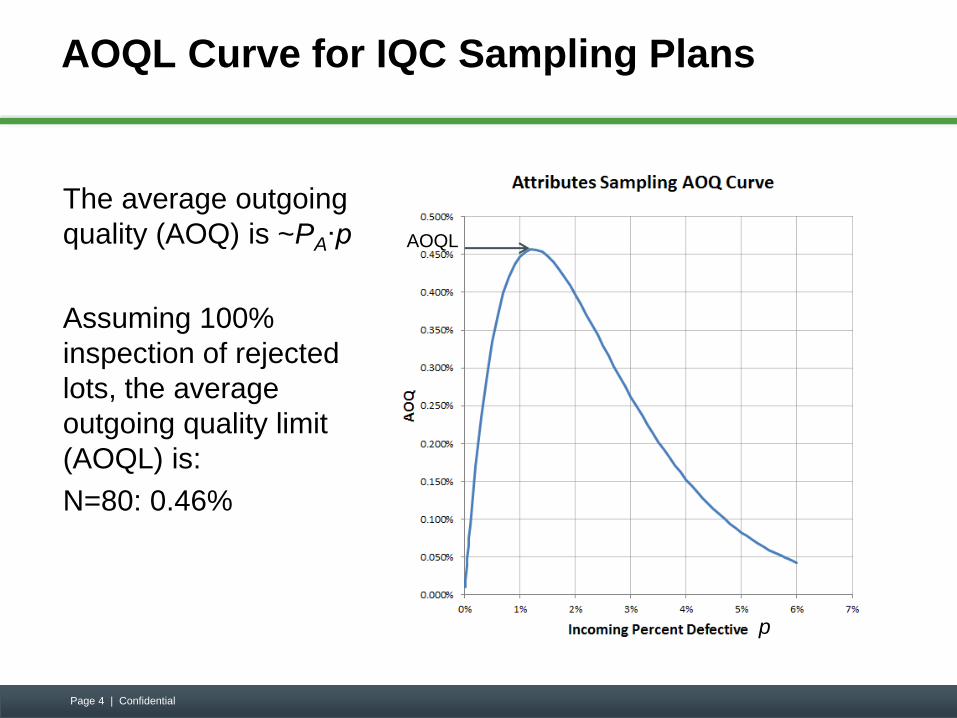
AOQL Curve for IQC Sampling Plans

The average outgoing

quality (AOQ) is ~PA∙p

Assuming 100%

inspection of rejected

lots, the average

outgoing quality limit

(AOQL) is:

N=80: 0.46%

| Confidential

p

AOQL

Proposal

The proposal was to employ variables sampling

plans that would result in a significant reduction in the

sample size inspection requirements compared to the

attributes sampling plans while providing equivalent

protection against bad batches.

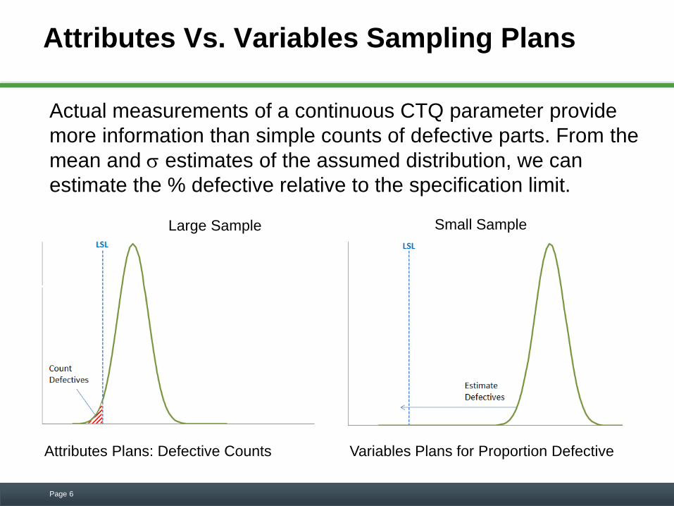
Attributes Vs. Variables Sampling Plans

Actual measurements of a continuous CTQ parameter provide

more information than simple counts of defective parts. From the

mean and estimates of the assumed distribution, we can

estimate the % defective relative to the specification limit.

Attributes Plans: Defective Counts Variables Plans for Proportion Defective

Large Sample Small Sample

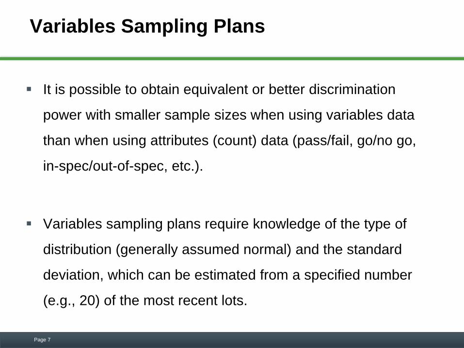
Variables Sampling Plans

It is possible to obtain equivalent or better discrimination

power with smaller sample sizes when using variables data

than when using attributes (count) data (pass/fail, go/no go,

in-spec/out-of-spec, etc.).

Variables sampling plans require knowledge of the type of

distribution (generally assumed normal) and the standard

deviation, which can be estimated from a specified number

(e.g., 20) of the most recent lots.

Acceptance Sampling by Variables

Variables Sampling Plans: For each CTQ, based on the estimated

(and assumed known) standard deviation, the specifications limits, the

AQL and RQL proportions defective and associated (producer’s) and

(consumer’s) risks, we determine a sample size n and an acceptance

mean K.

Single-Sided Limits: For a LSL, if the average of the n units is equal to

or above K, the CTQ passes. For an USL, if the average of the n units is

equal to or below K, the CTQ passes. If the average of the sample mean

is below K for a LSL or above K for an USL, the batch fails for this CTQ.

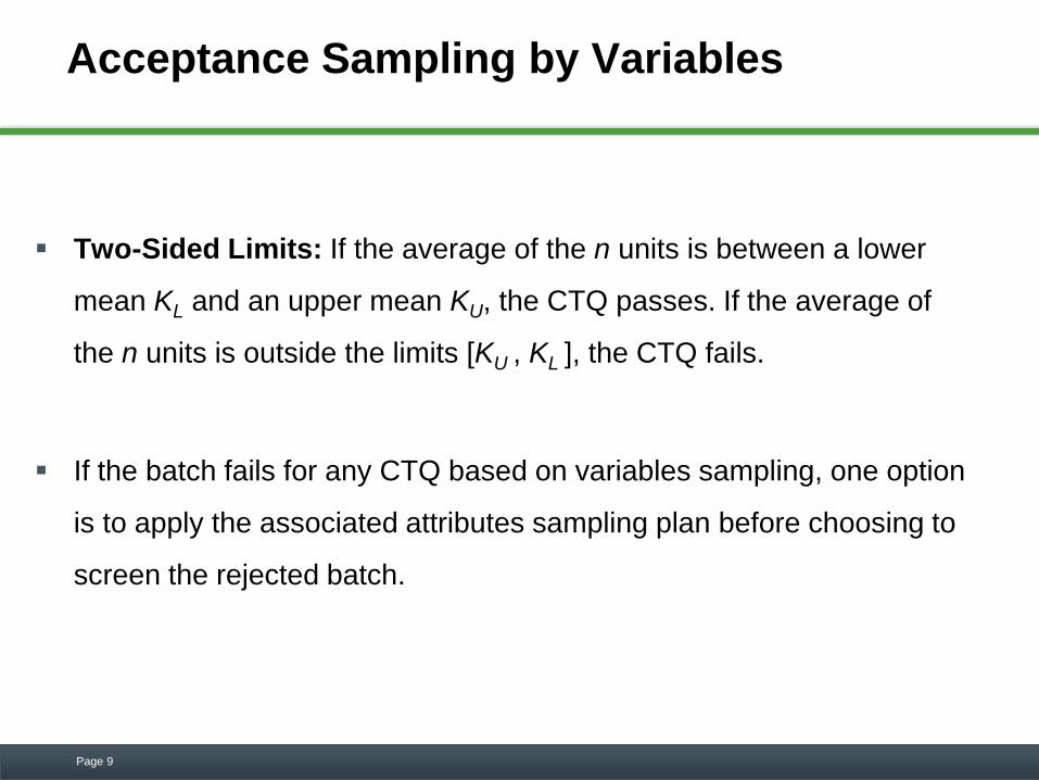
Acceptance Sampling by Variables

Two-Sided Limits: If the average of the n units is between a lower

mean KL and an upper mean KU, the CTQ passes. If the average of

the n units is outside the limits [KU , KL ], the CTQ fails.

If the batch fails for any CTQ based on variables sampling, one option

is to apply the associated attributes sampling plan before choosing to

screen the rejected batch.

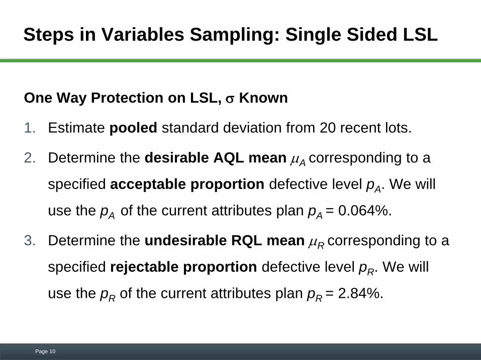
Steps in Variables Sampling: Single Sided LSL

One Way Protection on LSL, Known

1. Estimate pooled standard deviation from 20 recent lots.

2. Determine the desirable AQL mean A corresponding to a

specified acceptable proportion defective level pA. We will

use the pA of the current attributes plan pA = 0.064%.

3. Determine the undesirable RQL mean R corresponding to a

specified rejectable proportion defective level pR. We will

use the pR of the current attributes plan pR = 2.84%.



4. Specify the risk (producer’s risk) of rejecting a batch if the

true mean is the desirable mean. Typically = 5%.

5. Specify the risk (consumer’s risk) of accepting a batch if the

true mean is the undesirable mean. Typically = 10%.



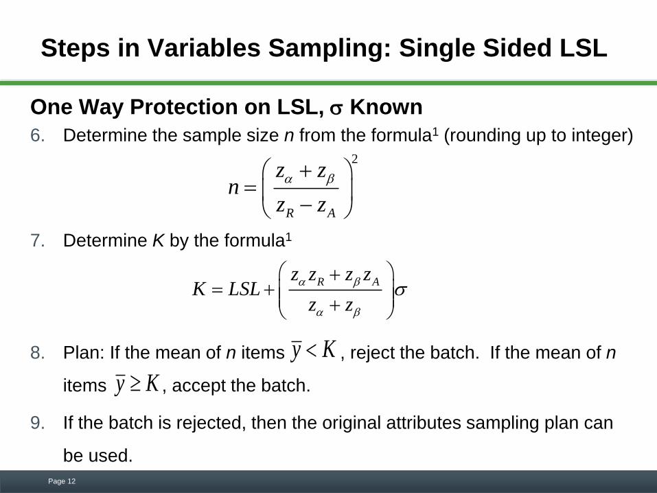
6. Determine the sample size n from the formula1 (rounding up to integer)

7. Determine K by the formula1

8. Plan: If the mean of n items , reject the batch. If the mean of n

items , accept the batch.

9. If the batch is rejected, then the original attributes sampling plan can

be used.

R Az z z zK LSL

z z

y K

y K

2

R A

z zn

z z

Measurement Error Analysis

It is important to periodically verify that a measurement system

analysis (gauge R&R) has been performed on the tools used to

measure CTQs.

The measurement error should be small enough to detect part to

part variation.

A measurement system analysis (MSA) can be performed in

JMP based on the EMP (Evaluating the Measurement Process)

analysis approach of Don Wheeler2.

Example X-Dim: JMP MSA

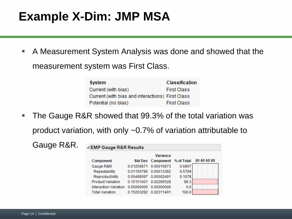
A Measurement System Analysis was done and showed that the

measurement system was First Class.

The Gauge R&R showed that 99.3% of the total variation was

product variation, with only ~0.7% of variation attributable to

Gauge R&R.

| Confidential

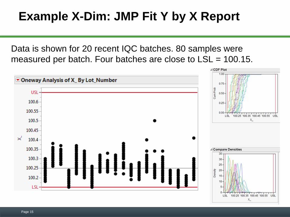
Example X-Dim: JMP Fit Y by X Report

Data is shown for 20 recent IQC batches. 80 samples were

measured per batch. Four batches are close to LSL = 100.15.

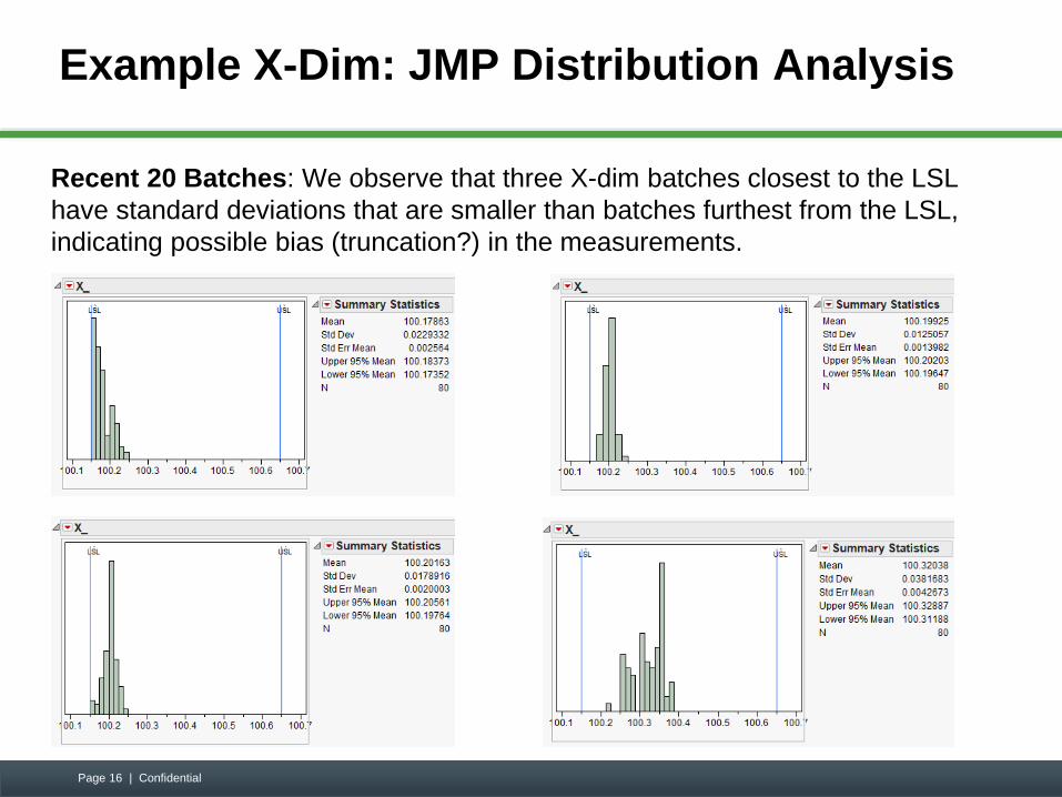
Example X-Dim: JMP Distribution Analysis

Recent 20 Batches: We observe that three X-dim batches closest to the LSL

have standard deviations that are smaller than batches furthest from the LSL,

indicating possible bias (truncation?) in the measurements.

| Confidential

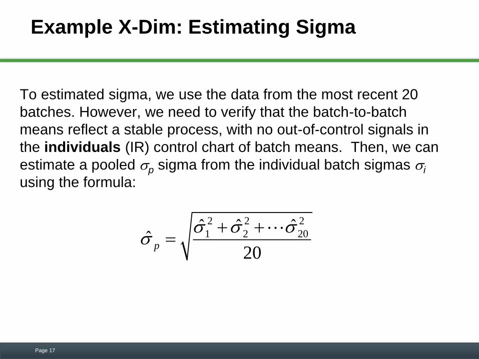
Example X-Dim: Estimating Sigma

To estimated sigma, we use the data from the most recent 20

batches. However, we need to verify that the batch-to-batch

means reflect a stable process, with no out-of-control signals in

the individuals (IR) control chart of batch means. Then, we can

estimate a pooled p sigma from the individual batch sigmas i

using the formula:

2 2 2

1 2 20ˆ ˆ ˆ

ˆ20

p

Example X-Dim: Batch-to Batch Process

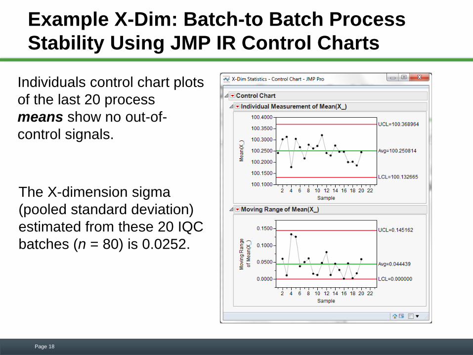
Stability Using JMP IR Control Charts

Individuals control chart plots

of the last 20 process

means show no out-of-

control signals.

The X-dimension sigma

(pooled standard deviation)

estimated from these 20 IQC

batches (n = 80) is 0.0252.

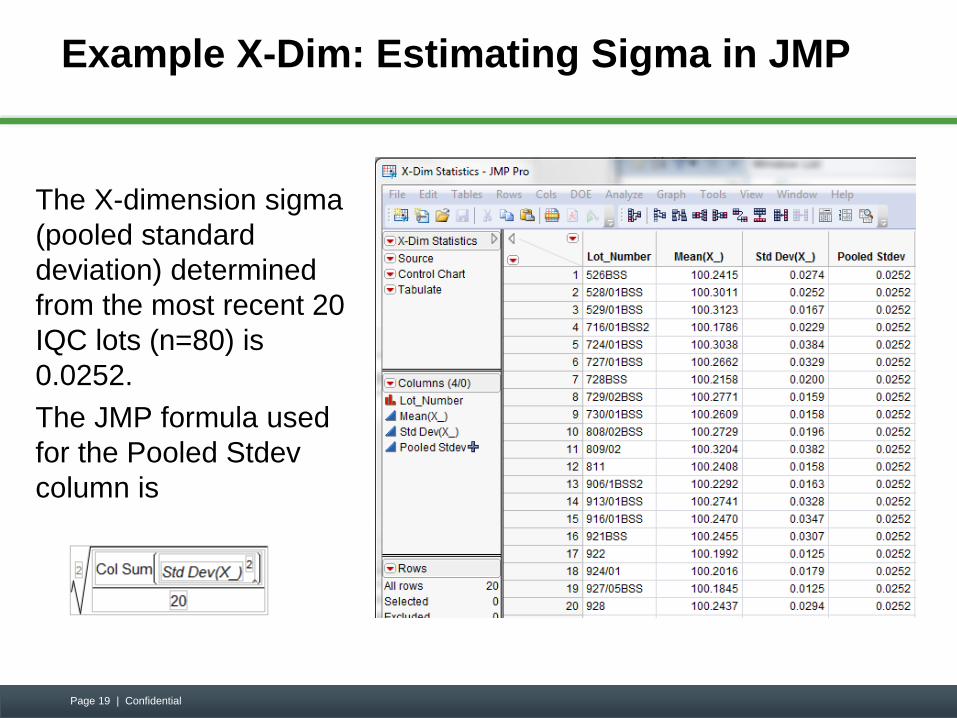
Example X-Dim: Estimating Sigma in JMP

The X-dimension sigma

(pooled standard

deviation) determined

from the most recent 20

IQC lots (n=80) is

0.0252.

The JMP formula used

for the Pooled Stdev

column is

| Confidential

Example X-Dim: Checking Normality

The data should also be checked to verify that the normal

distribution assumption is reasonable.

There are several reports in JMP that can be used as a

check for normality.

A simple analysis can be done in JMP’s Distribution

platform by selecting Normal Quantile Plot for the CTQ

measured. If the data points fall close to a straight line, the

normal distribution assumption is considered reasonable.

| Confidential

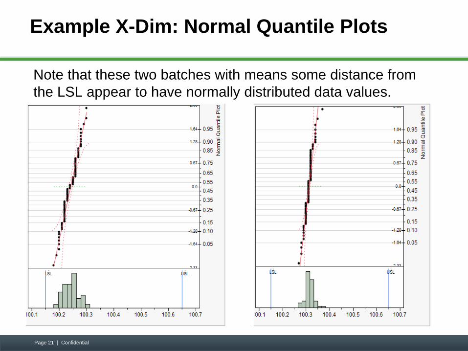
Example X-Dim: Normal Quantile Plots

Note that these two batches with means some distance from

the LSL appear to have normally distributed data values.

| Confidential

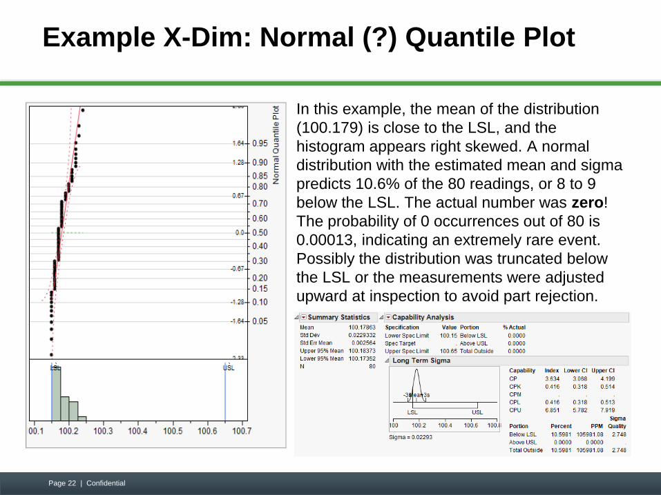
Example X-Dim: Normal (?) Quantile Plot

In this example, the mean of the distribution

(100.179) is close to the LSL, and the

histogram appears right skewed. A normal

distribution with the estimated mean and sigma

predicts 10.6% of the 80 readings, or 8 to 9

below the LSL. The actual number was zero!

The probability of 0 occurrences out of 80 is

0.00013, indicating an extremely rare event.

Possibly the distribution was truncated below

the LSL or the measurements were adjusted

upward at inspection to avoid part rejection.

| Confidential

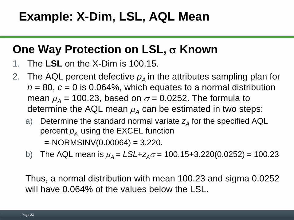
Example: X-Dim, LSL, AQL Mean


1. The LSL on the X-Dim is 100.15.

2. The AQL percent defective pA in the attributes sampling plan for

n = 80, c = 0 is 0.064%, which equates to a normal distribution

mean A = 100.23, based on = 0.0252. The formula to

determine the AQL mean A can be estimated in two steps:

a) Determine the standard normal variate zA for the specified AQL

percent pA using the EXCEL function

=-NORMSINV(0.00064) = 3.220.

b) The AQL mean is A = LSL+zA = 100.15+3.220(0.0252) = 100.23

Thus, a normal distribution with mean 100.23 and sigma 0.0252

will have 0.064% of the values below the LSL.

Example: X-Dim, LSL, RQL Mean


3. The RQL percent defective pR in the attributes sampling

plan for n = 80, c = 0 is 2.84%, which equates to a normal

distribution mean R = 100.198, for sigma of 0.0252. To

determine the corresponding mean R we find:

a) The standard normal variate zR for the specified RQL percent

pR using the EXCEL function

=-NORMSINV(0.0284) = 1.905.

b) The RQL mean is R = LSL+zR = 100.15+1.905(0.0252) =

100.198

Thus, a normal distribution with mean 100.198 and sigma

0.0252 will have 2.84% of the values below the LSL.

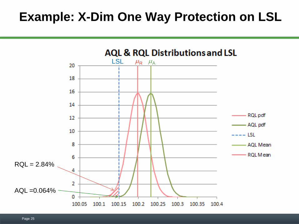
Example: X-Dim One Way Protection on LSL

RQL = 2.84%

AQL =0.064%

LSL R A

Steps in Variables Sampling


4. Determine the sample size from the formula1

5. Determine K

6. Plan: If the mean of 5 items is <100.2125, reject the

batch. If the mean of 5 items is > or = 100.2125, accept

the batch.

7. If the batch is rejected, the original attributes sampling

plan can be used.

2 21.645 1.282

~ 51.905 3.220R A

z zn

z z

1.645 1.905 1.282 3.220100.15 0.0252 100.2125

1.645 1.282

R Az z z zK LSL

z z

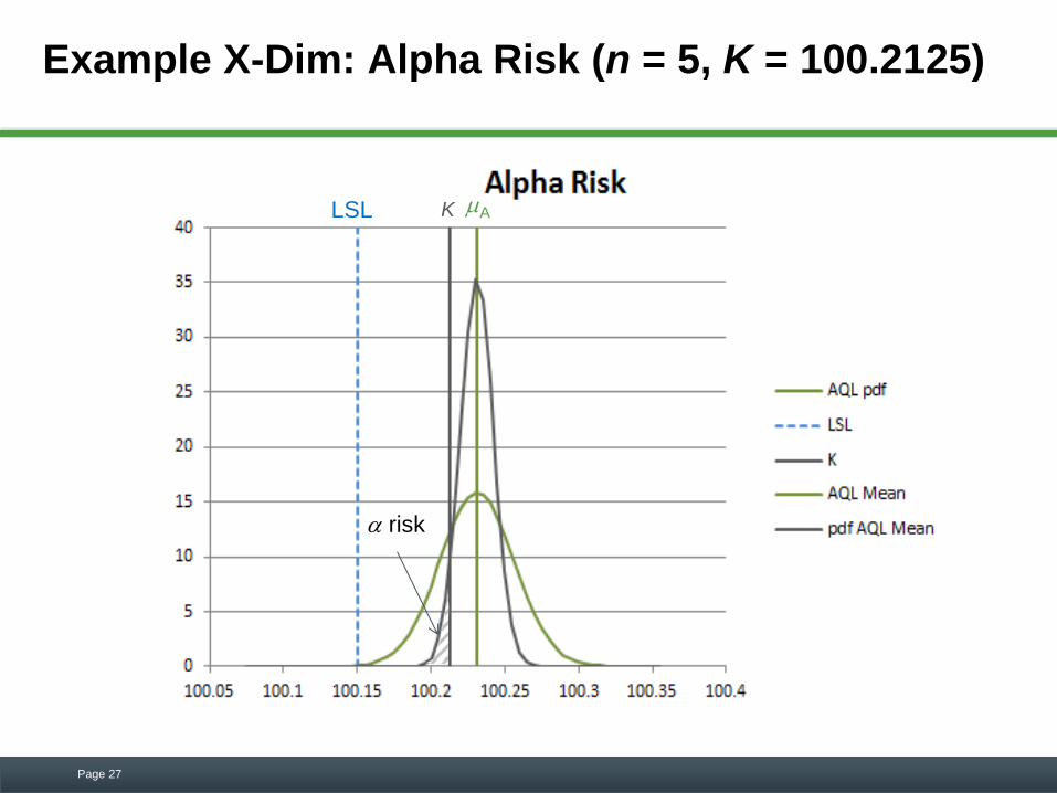
Example X-Dim: Alpha Risk (n = 5, K = 100.2125)

risk

LSL K A

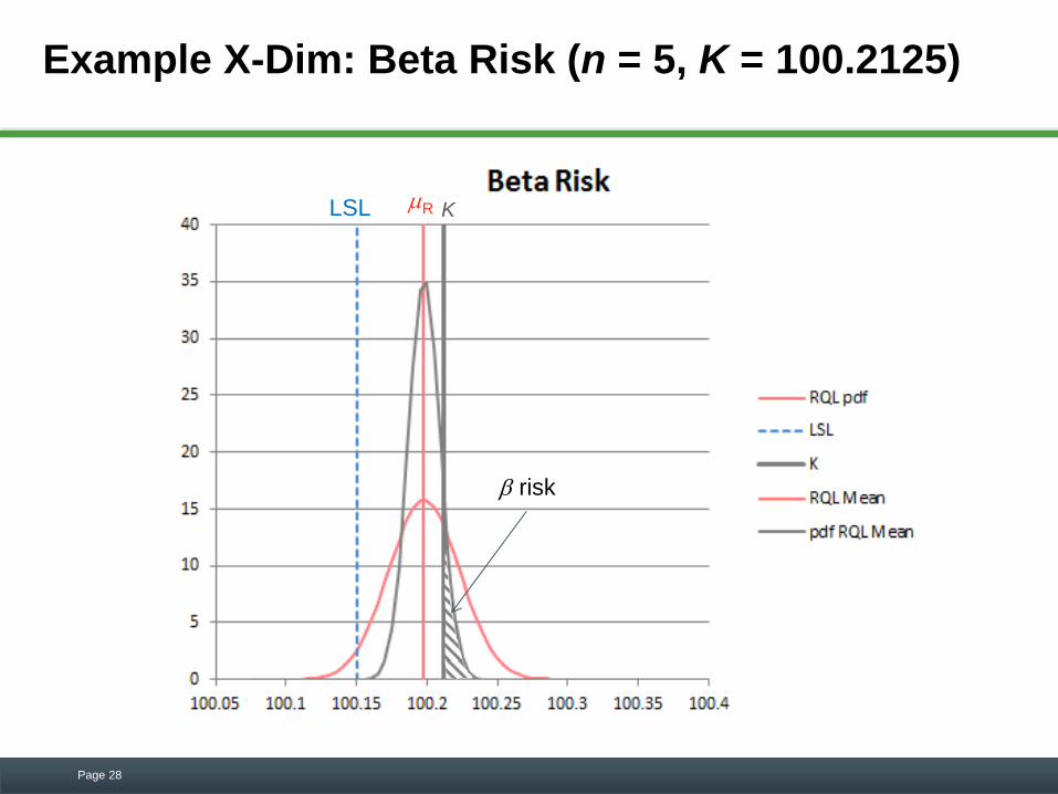
Example X-Dim: Beta Risk (n = 5, K = 100.2125)

risk

LSL K R

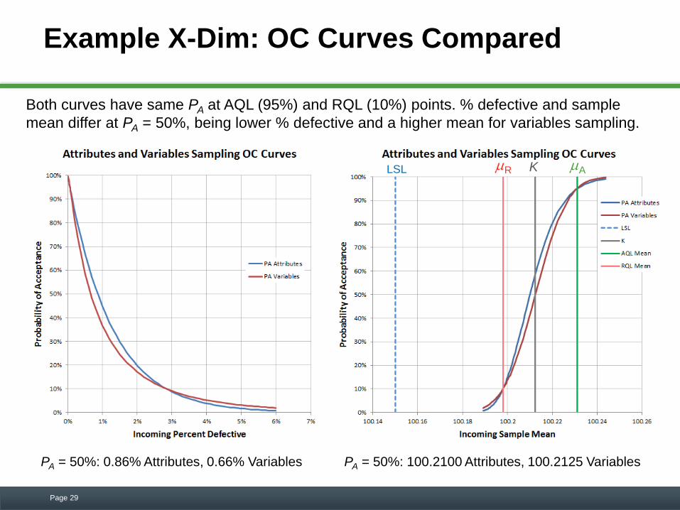
Example X-Dim: OC Curves Compared

Both curves have same PA at AQL (95%) and RQL (10%) points. % defective and sample

mean differ at PA = 50%, being lower % defective and a higher mean for variables sampling.

LSL R A K

PA = 50%: 0.86% Attributes, 0.66% Variables PA = 50%: 100.2100 Attributes, 100.2125 Variables

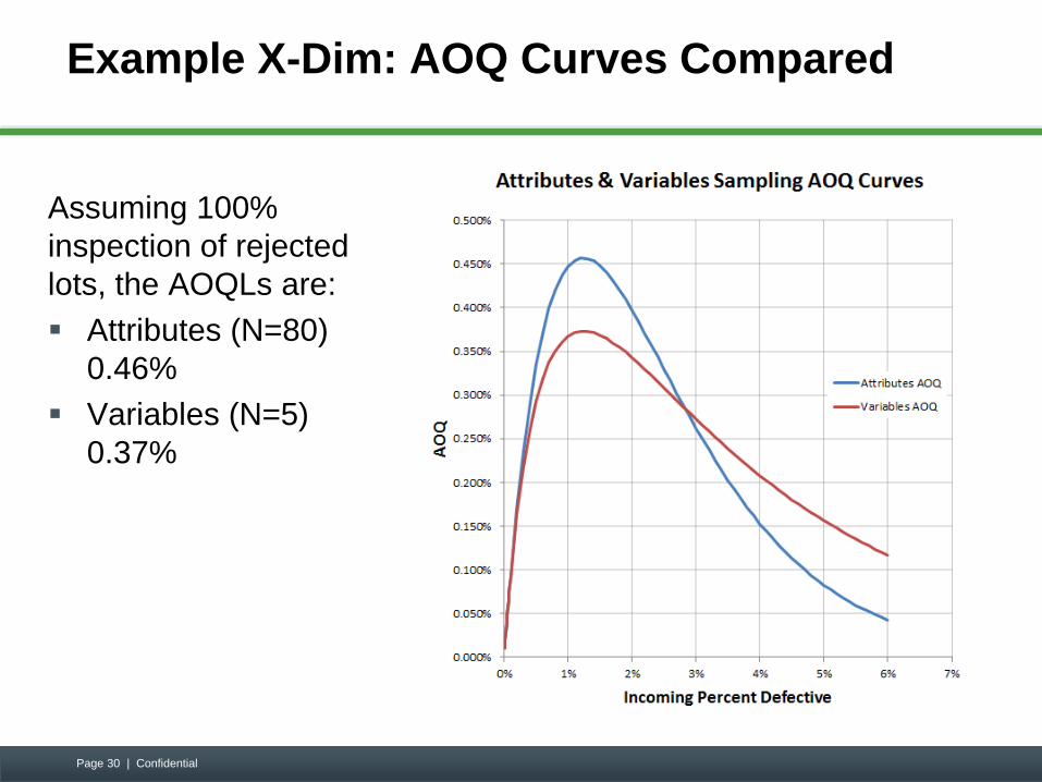
Example X-Dim: AOQ Curves Compared

Assuming 100%

inspection of rejected

lots, the AOQLs are:

Attributes (N=80)

0.46%

Variables (N=5)

0.37%

| Confidential

Example X-Dim: Application to Recent 20

Batches

As an application of the variables

approach, we will use the first five

measurements of the 20 recent batches,

which have 80 measurements per batch.

There are four means that fall below

K = 100.2125.

Thus, 4 batches out of 20 would require

the typical IQC attributes sampling of 80

measurements, a reduction of 80% in

batches needing extensive inspection.

The 16 batches with means above

K=100.2125 would be accepted based

on a sample size of 5, a reduction in

samples measured of ~94%.

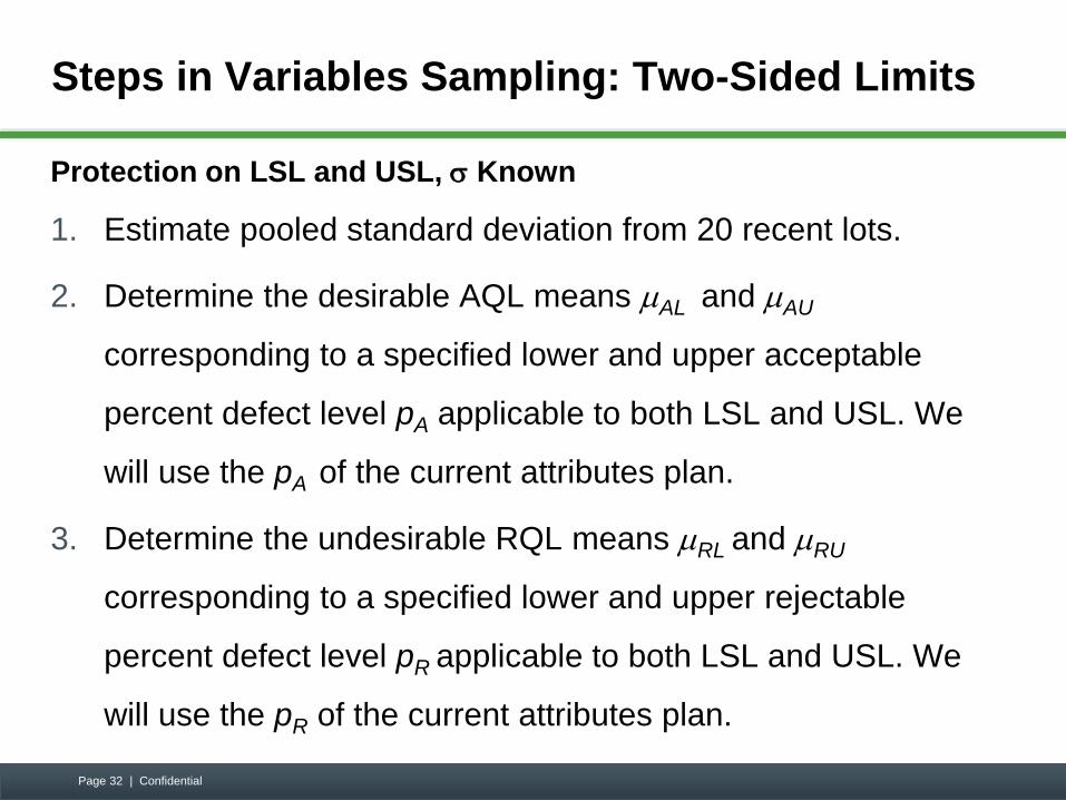
Steps in Variables Sampling: Two-Sided Limits

Protection on LSL and USL, Known

1. Estimate pooled standard deviation from 20 recent lots.

2. Determine the desirable AQL means AL and AU

corresponding to a specified lower and upper acceptable

percent defect level pA applicable to both LSL and USL. We

will use the pA of the current attributes plan.

3. Determine the undesirable RQL means RL and RU

corresponding to a specified lower and upper rejectable

percent defect level pR applicable to both LSL and USL. We

will use the pR of the current attributes plan.

| Confidential

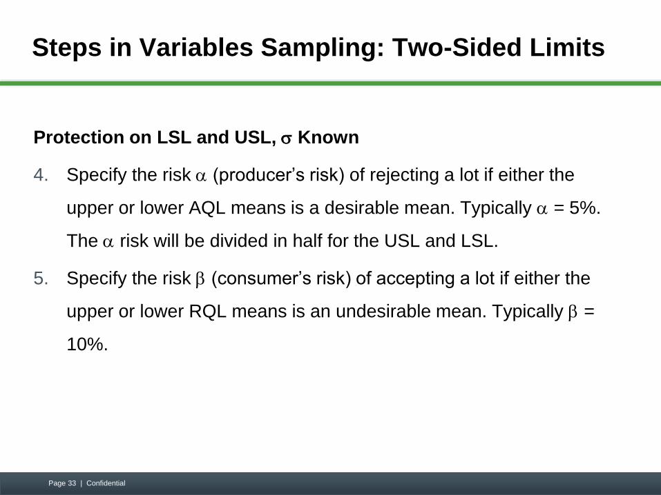
Steps in Variables Sampling: Two-Sided Limits


4. Specify the risk (producer’s risk) of rejecting a lot if either the

upper or lower AQL means is a desirable mean. Typically = 5%.

The risk will be divided in half for the USL and LSL.

5. Specify the risk (consumer’s risk) of accepting a lot if either the

upper or lower RQL means is an undesirable mean. Typically =

10%.

| Confidential

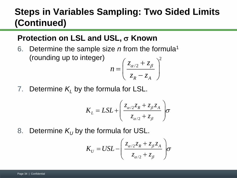
Steps in Variables Sampling: Two Sided Limits

(Continued)


6. Determine the sample size n from the formula1

(rounding up to integer)

7. Determine KL by the formula for LSL.

8. Determine KU by the formula for USL.

| Confidential

2

/2

R A

z zn

z z

/2

/2

R A

L

z z z zK LSL

z z

/2

/2

R A

U

z z z zK USL

z z

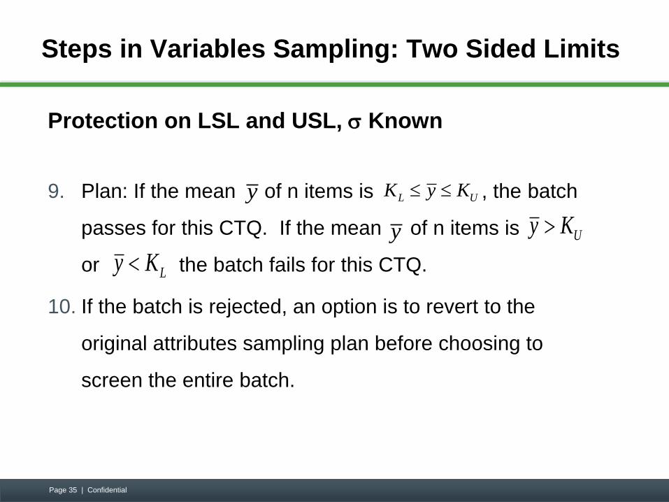
Steps in Variables Sampling: Two Sided Limits


9. Plan: If the mean of n items is , the batch

passes for this CTQ. If the mean of n items is

or the batch fails for this CTQ.

10. If the batch is rejected, an option is to revert to the

original attributes sampling plan before choosing to

screen the entire batch.

| Confidential

Ly K

Uy K

y L UK y K

y

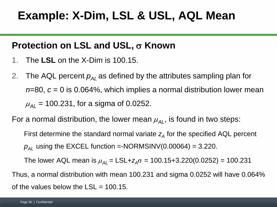
Example: X-Dim, LSL & USL, AQL Mean


1. The LSL on the X-Dim is 100.15.

2. The AQL percent pAL as defined by the attributes sampling plan for

n=80, c = 0 is 0.064%, which implies a normal distribution lower mean

AL = 100.231, for a sigma of 0.0252.

For a normal distribution, the lower mean AL, is found in two steps:

First determine the standard normal variate zA for the specified AQL percent

pAL using the EXCEL function =-NORMSINV(0.00064) = 3.220.

The lower AQL mean is AL = LSL+zA = 100.15+3.220(0.0252) = 100.231

Thus, a normal distribution with mean 100.231 and sigma 0.0252 will have 0.064%

of the values below the LSL = 100.15.

| Confidential

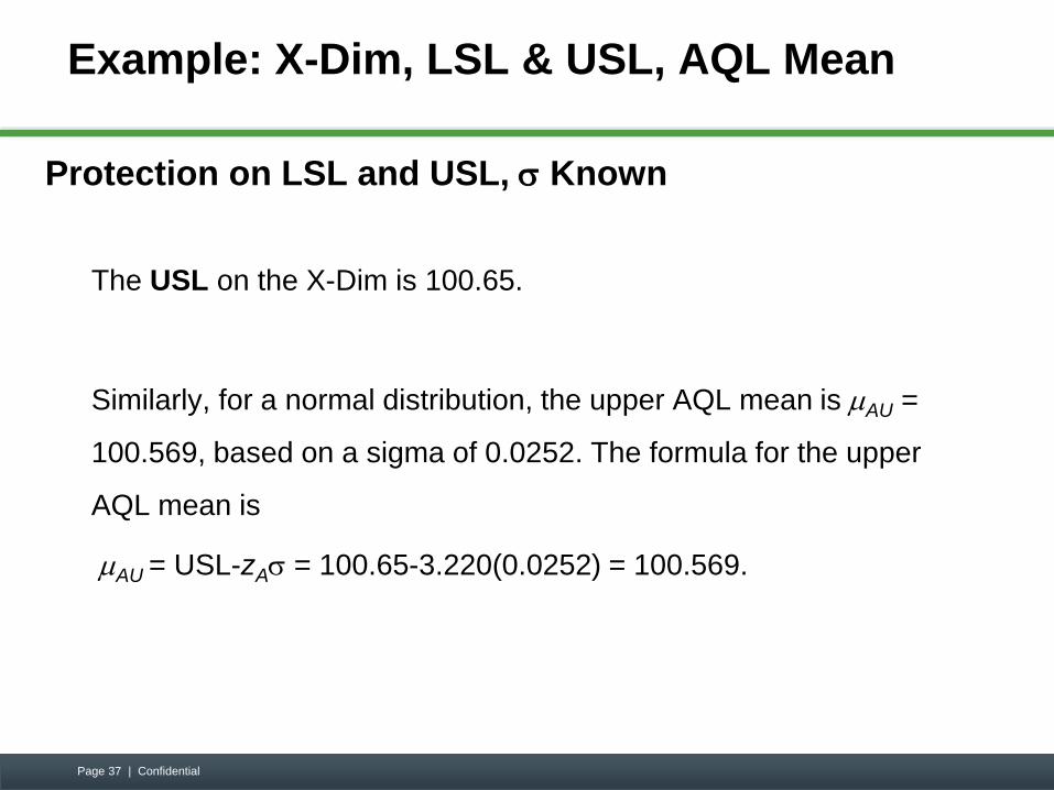
Example: X-Dim, LSL & USL, AQL Mean


The USL on the X-Dim is 100.65.

Similarly, for a normal distribution, the upper AQL mean is AU =

100.569, based on a sigma of 0.0252. The formula for the upper

AQL mean is

AU = USL-zA = 100.65-3.220(0.0252) = 100.569.

| Confidential

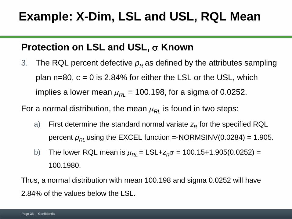
Example: X-Dim, LSL and USL, RQL Mean


3. The RQL percent defective pR as defined by the attributes sampling

plan n=80, c = 0 is 2.84% for either the LSL or the USL, which

implies a lower mean RL = 100.198, for a sigma of 0.0252.

For a normal distribution, the mean RL is found in two steps:

a) First determine the standard normal variate zR for the specified RQL

percent pRL using the EXCEL function =-NORMSINV(0.0284) = 1.905.

b) The lower RQL mean is RL = LSL+zR = 100.15+1.905(0.0252) =

100.1980.

Thus, a normal distribution with mean 100.198 and sigma 0.0252 will have

2.84% of the values below the LSL.

| Confidential

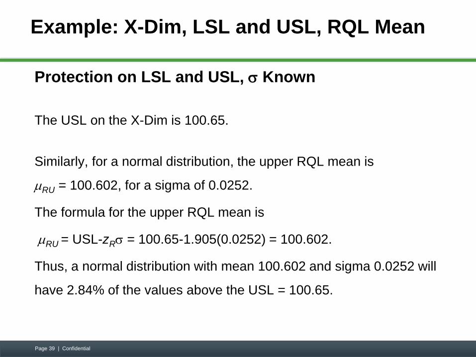
Example: X-Dim, LSL and USL, RQL Mean


The USL on the X-Dim is 100.65.

Similarly, for a normal distribution, the upper RQL mean is

RU = 100.602, for a sigma of 0.0252.

The formula for the upper RQL mean is

RU = USL-zR = 100.65-1.905(0.0252) = 100.602.

Thus, a normal distribution with mean 100.602 and sigma 0.0252 will

have 2.84% of the values above the USL = 100.65.

| Confidential

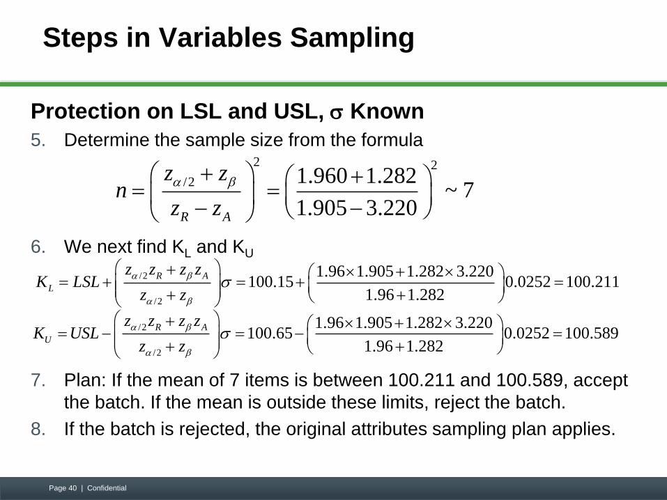
Steps in Variables Sampling


5. Determine the sample size from the formula

6. We next find KL and KU

7. Plan: If the mean of 7 items is between 100.211 and 100.589, accept

the batch. If the mean is outside these limits, reject the batch.

8. If the batch is rejected, the original attributes sampling plan applies.

| Confidential

2 2

/2 1.960 1.282~ 7

1.905 3.220R A

z zn

z z

/2

/2

1.96 1.905 1.282 3.220100.15 0.0252 100.211

1.96 1.282

R A

L

z z z zK LSL

z z

/2

/2

1.96 1.905 1.282 3.220100.65 0.0252 100.589

1.96 1.282

R A

U

z z z zK USL

z z

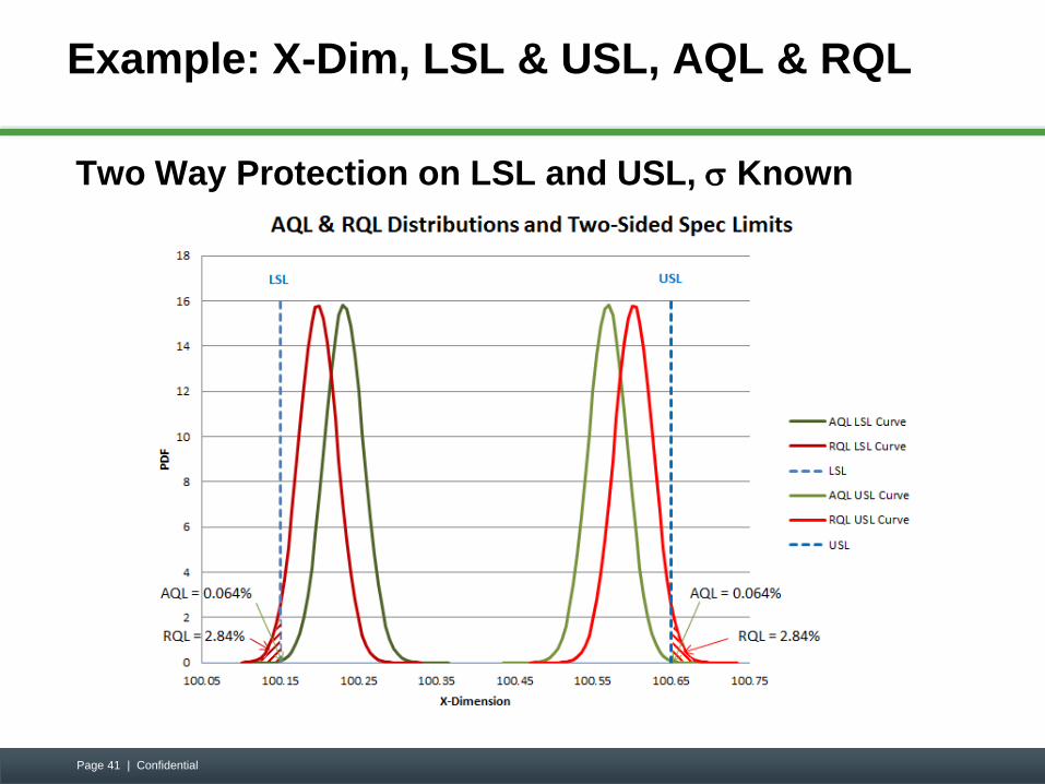
Example: X-Dim, LSL & USL, AQL & RQL

Two Way Protection on LSL and USL, Known

| Confidential

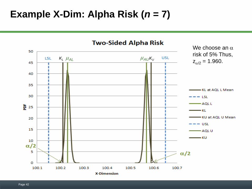
Example X-Dim: Alpha Risk (n = 7)

We choose an

risk of 5% Thus,

z/2 = 1.960. KL KU AL AU

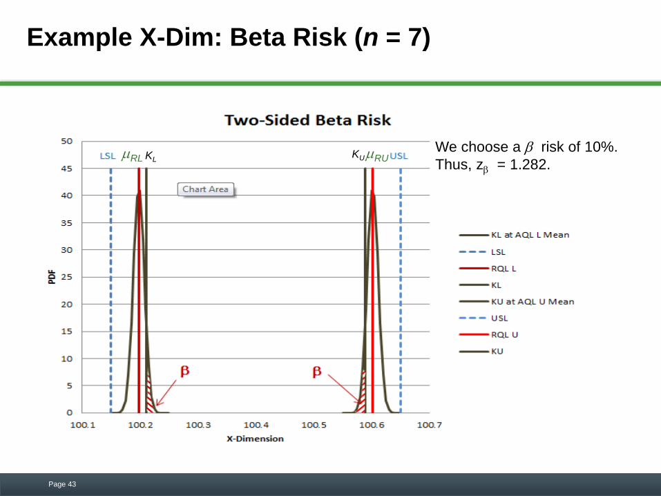
Example X-Dim: Beta Risk (n = 7)

We choose a risk of 10%.

Thus, z = 1.282. KL

KU RL RU

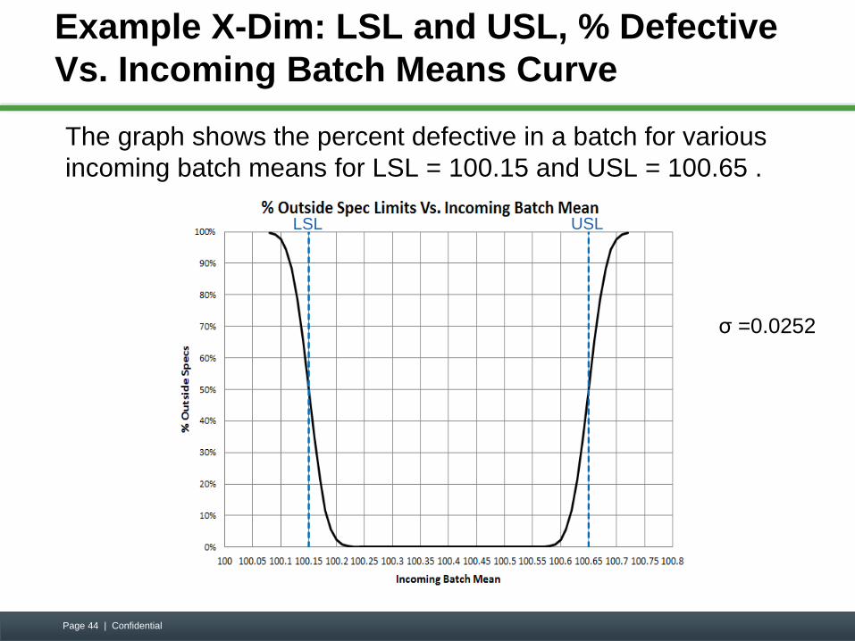
Example X-Dim: LSL and USL, % Defective

Vs. Incoming Batch Means Curve

The graph shows the percent defective in a batch for various

incoming batch means for LSL = 100.15 and USL = 100.65 .

| Confidential

LSL USL

σ =0.0252

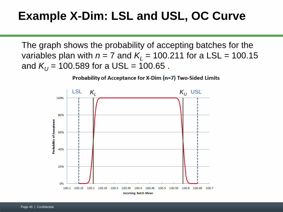
Example X-Dim: LSL and USL, OC Curve

The graph shows the probability of accepting batches for the

variables plan with n = 7 and KL = 100.211 for a LSL = 100.15

and KU = 100.589 for a USL = 100.65 .

| Confidential

LSL USL KL KU

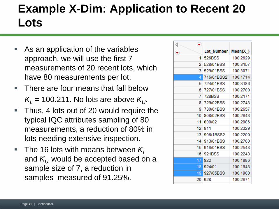
Example X-Dim: Application to Recent 20

Lots

As an application of the variables

approach, we will use the first 7

measurements of 20 recent lots, which

have 80 measurements per lot.

There are four means that fall below

KL = 100.211. No lots are above KU.

Thus, 4 lots out of 20 would require the

typical IQC attributes sampling of 80

measurements, a reduction of 80% in

lots needing extensive inspection.

The 16 lots with means between KL

and KU would be accepted based on a

sample size of 7, a reduction in

samples measured of 91.25%.

| Confidential

Summary

Variables sampling plans:

are based on the measurements rather than simple

count data of the number of rejectable parts

can provide equivalent or better protection compared

to attributes sampling plans

are based on assumptions that must be verified for

each CTQ

can significantly reduce samples sizes, time, and

costs for IQC inspection

References

1. Acceptance Sampling in Quality Control, 2nd ed.,

Edward G. Shilling, Dean V. Neubauer, 2009, CRC

Press, Taylor & Francis Group, Boca Raton, FL

2. EMPIII Evaluating the Measurement Process & Using

Imperfect Data, Donald J. Wheeler, 2006, SPC

Press, 5908 Toole Drive, Suite C, Knoxville, TB

37919

reduction of sampling inspection using variables …...reduction of sampling inspection using...

Documents