reduction of errors in digital terrain parameters used in soil-landscape modelling

International Journal of Applied Earth Observationand Geoinformation 5 (2004) 97–112

Reduction of errors in digital terrain parameters used insoil-landscape modelling�

Tomislav Hengla,∗, Stephan Gruberc, Dhruba P. Shresthaba Faculty of Agriculture, AGIS-Centre, Trg Sv. Trojstva 3, 31000 Osijek, Croatia

b International Institute for Geo-information Science and Earth Observation (ITC), P.O. Box 6, 7500 AA Enschede, The Netherlandsc Glaciology and Geomorphodynamics Group, Department of Geography, University of Zürich, Winterthurerstr. 190,

CH-8057 Zürich, Switzerland

Received 22 April 2003; accepted 20 January 2004

Abstract

Quality of digital elevation models (DEMs) and DEM-derived products directly affects the quality of terrain analysis appli-cations. The objective of this work was to review and systematise methods to improve geomorphic plausibility of DEMs andminimise artefacts and outliers in terrain parameters. Three approaches to the reduction of errors in DEM and DEM-derivedproducts are described: (a) by using empirical knowledge, e.g. to adjust elevations using medial axes or stream networks; (b) byapplying filtering operations and (c) by averaging terrain parameters derived from multiple realisations of DEM, i.e. using errorpropagation technique. The methods were tested using a 3.8×3.8 km sample area covering two distinct landscapes: hilland andplain with terraces. The DEM was produced by linear interpolation of contour data. The proportion of artefacts (padi terraces)in the unfiltered DEM was 17.3%. After the addition of medial axes, filtering of outliers and adjustment of elevation for streams,the proportion of padi terraces was reduced to 2.2%. Remaining errors in terrain parameters such as undefined pixels and localoutliers were reduced using repeated filtering (with iterations). All terrain parameters were also calculated by averaging multi-ple realisations. Both the filtering approach and averaging multiple realisations give somewhat smoother maps of terrain param-eters. The advantage of filtering of outliers is that it employs the spatial autocorrelation structure. The advantage of averagingmultiple realisations is that it can be easier automated. The reduction of errors improved the mapping of landform facets (classi-fication) and solum thickness (regression). The classification accuracy increased from 51.3 to 72% and theR2 of the regressionmodel for the prediction of the solum thickness increased from 0.27 to 0.40. These methods can be used to filter DEMs derivedfrom contour data and terrain parameters, but also to reduce errors in other types of gridded DEMs and DEM-derived products.© 2004 Elsevier B.V. All rights reserved.

Keywords:Terrain analysis; Digital Elevation Model; Filtering; Geostatistical simulation; Contours

� Supplementary materials: datasets, animations, lecture note“Digital terrain analysis inILWIS”, p. 53, available on-line at:http://www.itc.nl/personal/shrestha/DTA/.∗ Corresponding author. Tel.:+385-31-224288;

fax: +385-31-207017.E-mail addresses:[email protected] (T. Hengl),

[email protected] (S. Gruber), [email protected](D.P. Shrestha).

1. Introduction

Digital terrain parameters, also known as topo-graphic attributes(Wilson et al., 2000)or morpho-metric variables(Shary et al., 2002)are commonlyderived from the digital elevation model (DEM) usingsome digital terrain analysis method. There has beenan increasing interest in the use of relief data in the

0303-2434/$ – see front matter © 2004 Elsevier B.V. All rights reserved.doi:10.1016/j.jag.2004.01.006

http://www.itc.nl/personal/shrestha/DTA/

98 T. Hengl et al. / International Journal of Applied Earth Observation and Geoinformation 5 (2004) 97–112

last decade accompanied by a growing availability ofDEMs. The quality of terrain parameters is importantas it directly affects the quality of spatial modelling.Several factors play an important role for the qualityof DEM-derived products(Thompson et al., 2000):

• terrain roughness and complexity;• terrain modelling aspects—sampling density, DEM

collection and interpolation method;• grid spacing or pixel size;• vertical resolution or precision;• type and nature of algorithms used to derive terrain

parameters.

Under slightly different input factors, e.g. coarser gridresolutions, vertical resolution or different filter algo-rithms, the terrain analysis can result in fundamen-tally different features(Wilson et al., 2000). The im-portance of each factor, however, is usually driven byapplication-specific rules(Martinoni, 2002).

A large group of terrain analysis applications is re-lated to mapping and modelling of soil data. Terrainparameters are most commonly used as extensivelymapped secondary or auxiliary variables to improvespatial prediction of soil-scapes and soil properties,such as thicknesses of horizons and other chemical(e.g. pH, organic matter) and physical (e.g. particlesize fractions) properties(Moore et al., 1993; Gessleret al., 1995; McKenzie and Ryan, 1999). The applica-tion of statistical techniques for analysis of spatial dis-tribution of soils using terrain and other environmentalparameters is commonly referred to assoil-landscapemodelling(McKenzie et al., 2000). In many cases, theerrors in terrain parameters or terrain analysis algo-rithms are not considered as a quality control factorfor successful soil-landscape modelling.

1.1. Errors in terrain parameters

For digital terrain analysis it is more importanthow well a DEM resembles actual terrain shapes andflow/deposition processes than what is the absoluteaccuracy of the elevation values. This resemblance isoften referred to as therelative accuracyof DEMs(Wise, 2000). Whereas absolute accuracy denotes thefit between the DEM and the real world, relative accu-racy is a measure of the quality of DEM-derived prod-ucts. Thus, the accuracy of terrain parameters is “less afunction of absolute accuracy of elevation values than

of how well and how smoothly the landscape featuresare modeled”(MacMillan et al., 2000). Schneider(1998) introduced the term “geomorphologicalplausibility” to denote a compromise between the ge-omorphologic knowledge, sampled elevation data andinterpolation techniques. In practice, field validationof accuracy of terrain parameters (e.g. hand measure-ments of slope, aspect and curvatures) has proven to bedifficult due to the fractal nature of topography and ab-stract definition of many terrain parameters(Florinsky,1998). The process of detecting and reducing errors istherefore somewhat different from detection of errorsin remote sensing or other GIS data sources.

The errors in DEM and DEM-derived productscan be roughly grouped in three types: (i) artefacts,blunders or gross errors, (ii) systematic errors and(iii) random errors or noise(Wise, 2000). Artefactsin terrain parameters are usually harder to detect inthe input DEM, but they will certainly be visible inDEM-derived products. For example, interpolation ofdigitised contour lines using the linear interpolatorwill typically show artefacts in the slope and as-pect maps (Dakowicz and Gold, 2002; Burrough andMcDonnell, 1998, p. 127). The most typical artefactsare the so-called ‘padi’ or ‘rice’ terraces or cut-offs,which are absolutely flat. Although these are notvisible in the DEM, the calculation of aspect or Com-pound Topographic Index (CTI) fails due to divisionby zero, which finally results in part of the area beingundefined. The padi terraces are somewhat similar toclouded pixels in remote sensing images, which sug-gests that similar geostatistical procedures (kriging orco-kriging) can be applied to remove them(Addinkand Stein, 1999). Other common artefacts are ‘ghost’lines or ‘tiger stripes’, which are obviously erratic fea-tures (Burrough and McDonnell, 1998). Systematicerrors reflect the limitations of an algorithm and canbe detected as local, unrealistic features or outliers.

Errors are especially common for terrain parame-ters derived using the higher order derivatives (curva-tures), aspect map and hydrological parameters (CTI).Wise (2000)gives a comparison of different interpola-tion techniques and terrain analysis algorithms whenapplied in calculation of hydrological parameters.Thompson et al. (2000)evaluated the effect of thechange in resolution on soil-landscape modelling andshowed that with the increase of pixel size, spatial pre-diction of soil variables will be less discernible, while

T. Hengl et al. / International Journal of Applied Earth Observation and Geoinformation 5 (2004) 97–112 99

decreased vertical precision will typically show moreerratic values.Wilson et al. (2000)emphasized theimportance of the finer grid resolutions and flexiblealgorithms using a set of studies.Tang et al. (2002),showed that accuracy of DEM-derived hydrologicaldata is directly related to DEM vertical resolution andterrain roughness. In the areas where the slope wasless than four degrees, the hydrological parameterswere usually unreliable.Florinsky (1998)investigatedthe influence of different algorithms used to derive ter-rain parameters on the overall precision.Holmes et al.(2000) showed that local inaccuracies in the USGS30 m DEM can be large and that the highest impactof the errors on terrain parameters is in the valleybottoms.

In many cases, even simple smoothing of DEMshas proven to be beneficial in improving the qualityof terrain parameters(Wise, 2000). Brown and Bara(1994)used low-pass filters in combination with anal-ysis of spatial dependence to reduce outliers in ele-vation, slope and curvatures.MacMillan et al. (2000)described a set filtering procedures to account for lo-cal noise and optimise terrain surfacing. Several otherstatistical image processing methods for reduction oferrors have been proposed(Felicisimo, 1994; Lopez,2000). In hydrological applications, quality of terrainparameters is usually improved by adjusting the inter-polation to the existing network of streams and ridgesor by removing the sinks. The automatic adjustmentof DEMs has been implemented, for example, in theANUDEM program (Hutchinson, 1989). However,ANUDEM and similar algorithms do not necessarilyguarantee reduction of padi terraces, local outliersand other artefacts. There is still a need for flexiblemethods to improve plausibility of DEMs derivedfrom contour lines. In addition, systematic methodol-ogy to quantify and reduce errors in number of mor-phometric and hydrological terrain parameters is stilllacking.

In this paper, we describe a set of systematicmethods that can be used in a raster-based GISto reduce errors in gridded DEMs (array of pixelsat regular square grid) and DEM-derived products.We compared different existing methods that canbe used to reduce errors and suggested some newtechniques. These are based on both empirical andstatistical assumptions on the nature of terrain pa-rameters. We focus mainly on digital terrain analysis

algorithms applied to elevation data derived fromcontour lines and soil-landscape modelling applica-tions. Note that we use filtering and neighbourhoodGIS operations as applied in Integrated Land andWater Information System (ILWIS) GIS package. Fordetailed description of algorithms used inILWIS seeHengl et al. (2003).

2. Methods

Let the elevation map be denoted asz or DEM, ter-rain parameters denoted asτ or TP and errors denotedase, wherezi is the elevation value atith grid loca-tion (z1, z2, . . . , zn) andn is the number of pixels ina map. A realisation of elevation map is then denotedz∗ andz∗j is thejth realisation of elevation map andfiltered map is denotedz+. Let also the derivation ofterrain parameter from elevation be denoted asτ(z)

or TP(DEM) and local neighbourhood be denoted aszNB. In a k × k window environment,zNB× is thevalue of the central cell andzNBc is the value at thecth neighbour of itsk2 neighbours. Commonly usedwindow sizes are 3× 3 and 5× 5.

2.1. Detection and quantification of errors

Prior to the calculation of terrain parameters, itis important to first detect and reduce errors in theDEM (Wise, 2000). The first errors we need to reduceare the padi terraces or cut-offs. These are the areaswhere all surrounding pixels show the same value andcan be defined as

e← [∀c zNBc = zNB×] (1)

Padi terraces are typical for closed contour lines andlinear interpolators but can also appear when smootherinterpolators are used. This happens because the hilltops, small ridges and valley bottoms are typicallynot recorded in the topo-map or no elevation valueis attached to them. In a GIS, padi terraces can bedetected using a neighbourhood operation.

Second type of errors that need to be detected arelocal outliers. These can be defined as small, veryunprobable features, which could have happen dueto the gross error in the data collection method (verycommon for remote-sensing based instruments) orinterpolation algorithm. They can be detected and


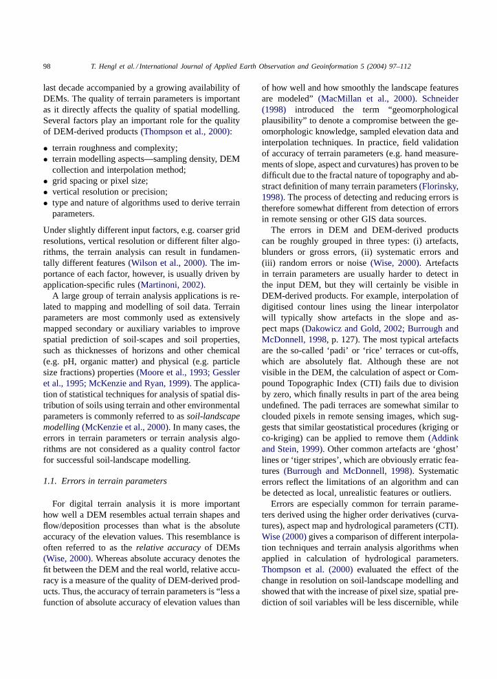
Fig. 1. Chematic examples of filtering environments assumingisotropic model: (a) 3× 3 window environment with commondesignation of neighbours and (b) 5×5 window environment withweights. The weights are used to predict the central pixel.

quantified by using the statistical approach suggestedby Felicisimo (1994). In this case, the probability tofind a certain value within the neighbourhood is cal-culated by comparing the original elevation with thevalue estimated from the neighbours:

δi = zNBi − zi (2)

where δi is the difference between the original andestimated value andzNB

i is the elevation (or terrainparameter) estimated from the neighbours. A statis-tically sound method to estimate the central valuefrom the neighbouring pixels is to use the spatial de-pendence structure, i.e. predict the central value bykriging (Felicisimo, 1994). In a 3× 3 window envi-ronment, assuming the isotropic variation, there areonly two types of distances: in the cardinal (2, 4, 6,8) and diagonal directions (1, 3, 7, 9) (Fig. 1a) . Analternative is to use the 5× 5 window size with 24neighbours and five types of weights (Fig. 1b).

In a 3× 3 window, the predictions are made by

zNB = wB[zNB1+ zNB3+ zNB7+ zNB9]

+wA[zNB2+ zNB4+ zNB6+ zNB8] (3)

wherewA is the weight in cardinal direction andwB isthe weight in diagonal direction. In general case (k×kwindow), the predictions are made by

zNB =k2∑c=1

wc × zNBc;k2∑c=1

wc = 1 (4)

wherewc is the weight atcth neighbour andw× is theweight at the central pixel, so thatw× = 0 and× =(k2+1)/2. Note that in the case of anisotropy, differentweights can be used in different directions. The (krig-ing) weights are solved using the covariance functionand relative distances between all pixels(Isaaks andSrivastava, 1989).

The difference between estimated and true value iscalculated for each pixel to derive overall average andstandard deviation (δ and sδ). Assuming a Gaussiandistribution, Student’st test is used to standardise thedifferences by

ti = δi − δsδ; i = 1, . . . , n (5)

wheren is the total number of pixels. Note that theoverall average of differences should equal zero. Theoutliers (e) are then detected as

ei← [|ti| ≥ tα/2,n−2] (6)

For the two-tail 99.9% probability (a = 0.01) t hasvalue of 3.219.

2.2. Reduction of errors

2.2.1. Improving the plausibility of DEMsPrior to actual filtering of terrain parameters, it is

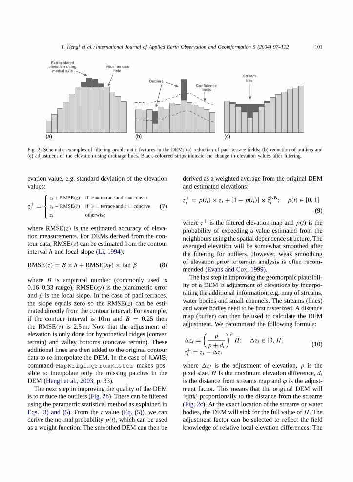
advisable to improve the plausibility of the DEM.The first step in improving the DEMs derived fromthe contour data is to account for features not shownby the contours such as break-lines indicating ridgesor valley bottoms. This can be achieved by digitizingsupplementary contour lines and spot heights repre-senting small channels, hilltops and ridges that are notindicated on the original topographic maps but can beinferred. The proportion of artefacts can be fairly high,especially in flat terrains, which means that the manualdigitization can be a time consuming process. An al-ternative is the automated detection of medial axes be-tween the closed contour lines. These are hypotheticalridges or valley bottoms, also called ‘skeleton-lines’(Fig. 2a). First, the padi terraces need to be detectedusingEq. (1). Then the medial axes can be detectedusing a distance operation from the bulk contourdata(Pilouk and Tempfli, 1992). The new elevationis assigned to the medial axes between the closedcontours by adding or subtracting some threshold el-


OutliersConfidence

limits

Streamline

‘Rice’ terrace field

Extrapolatedelevation using

medial axis

(a) (b) (c)

Fig. 2. Schematic examples of filtering problematic features in the DEM: (a) reduction of padi terrace fields; (b) reduction of outliers and(c) adjustment of the elevation using drainage lines. Black-coloured strips indicate the change in elevation values after filtering.

evation value, e.g. standard deviation of the elevationvalues:

z+i =zi + RMSE(z) if e = terrace andτ = convex

zi − RMSE(z) if e = terrace andτ = concave

zi otherwise

(7)

where RMSE(z) is the estimated accuracy of eleva-tion measurements. For DEMs derived from the con-tour data, RMSE(z) can be estimated from the contourintervalh and local slope(Li, 1994):

RMSE(z) = B× h+ RMSE(xy)× tan β (8)

where B is empirical number (commonly used is0.16–0.33 range), RMSE(xy) is the planimetric errorandβ is the local slope. In the case of padi terraces,the slope equals zero so the RMSE(z) can be esti-mated directly from the contour interval. For example,if the contour interval is 10 m andB = 0.25 thenthe RMSE(z) is 2.5 m. Note that the adjustment ofelevation is only done for hypothetical ridges (convexterrain) and valley bottoms (concave terrain). Theseadditional lines are then added to the original contourdata to re-interpolate the DEM. In the case ofILWIS,commandMapKrigingFromRaster makes pos-sible to interpolate only the missing patches in theDEM (Hengl et al., 2003, p. 33).

The next step in improving the quality of the DEMis to reduce the outliers (Fig. 2b). These can be filteredusing the parametric statistical method as explained inEqs. (3) and (5). From thet value (Eq. (5)), we canderive the normal probabilityp(t), which can be usedas a weight function. The smoothed DEM can then be

derived as a weighted average from the original DEMand estimated elevations:

z+i = p(ti)× zi + [1− p(ti)] × zNBi ; p(t) ∈ [0,1]

(9)

wherez+ is the filtered elevation map andp(t) is theprobability of exceeding a value estimated from theneighbours using the spatial dependence structure. Theaveraged elevation will be somewhat smoothed afterthe filtering for outliers. However, weak smoothingof elevation prior to terrain analysis is often recom-mended(Evans and Cox, 1999).

The last step in improving the geomorphic plausibil-ity of a DEM is adjustment of elevations by incorpo-rating the additional information, e.g. map of streams,water bodies and small channels. The streams (lines)and water bodies need to be first rasterized. A distancemap (buffer) can then be used to calculate the DEMadjustment. We recommend the following formula:

�zi =(

p

p+ di

)ϕH; �zi ∈ [0, H ]

z+i = zi −�zi(10)

where�zi is the adjustment of elevation,p is thepixel size,H is the maximum elevation difference,diis the distance from streams map andϕ is the adjust-ment factor. This means that the original DEM will‘sink’ proportionally to the distance from the streams(Fig. 2c). At the exact location of the streams or waterbodies, the DEM will sink for the full value ofH . Theadjustment factor can be selected to reflect the fieldknowledge of relative local elevation differences. The


maximum elevation difference can be estimated fromthe field knowledge or an arbitrary small number canbe used, e.g. half the contour intervalh. This meansthat for h = 10 m the adjustment of elevation for<5 m does not affect the original position of contours.

The suitable grid resolution can be estimated fromthe bulk contour data by using the total length of con-tours. As a rule of thumb, grid resolution (p) shouldbe at least half the average spacing between the con-tours (for detailed elaboration see (Hengl et al., 2003,pp. 8–11)):

p = A

2∑L

(11)

whereA is the total size of the study area and∑L is

the total cumulative length of digitised contours. Al-ternatively, the grid resolution can be estimated usingcartographic standards. According toTempfli (1999),the grid resolution should be optimally the maximumgraphic resolution of lines shown on the maps, i.e.0.4 mm at map scale. In the case of both estimatingthe pixel size and vertical resolution of the DEM, it isadvisable to round down the numbers—the finer thegrid size the better!

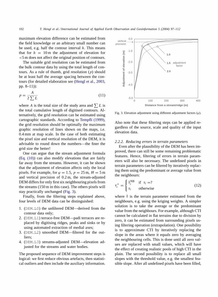
One can argue that the stream adjustment formula(Eq. (10)) can also modify elevations that are fairlyfar away from the streams. However, it can be shownthat the adjustment of elevation affects only the localpixels. For example, forϕ = 1.5,p = 25 m,H = 5 mand vertical precision of 0.2 m, the stream-adjustedDEM differs for only first six neighbouring pixels fromthe streams (150 m in this case). The others pixels willstay practically unchanged (Fig. 3).

Finally, from the filtering steps explained above,four levels of DEM data can be distinguished:

1. (DEM L0) the unfiltered DEM—derived from thecontour data only;

2. (DEM L1) terrace-free DEM—padi terraces are re-placed by digitising ridges, peaks and sinks or byusing automated extraction of medial axes;

3. (DEM L2) smoothed DEM—filtered for the out-liers;

4. (DEM L3) streams-adjusted DEM—elevation ad-justed for the streams and water bodies.

The proposed sequence of DEM improvement steps islogical: we first reduce obvious artefacts, then statisti-cal outliers and then include the auxiliary information.

-5.0

-4.0

-3.0

-2.0

-1.0

0.0

0 100 200 300 400

Distance from a stream/ridge (m)

Ad

just

men

to

fel

evat

ion

(m)

1.0

1.5

2.0

verticalprecision

adjustmentfactor

Fig. 3. Elevation adjustment using different adjustment factors (ϕ).

Also note that these filtering steps can be applied re-gardless of the source, scale and quality of the inputelevation data.

2.2.2. Reducing errors in terrain parametersEven after the plausibility of the DEM has been im-

proved, there can still be some remaining problematicfeatures. Hence, filtering of errors in terrain param-eters will also be necessary. The undefined pixels interrain parameters can be filtered by iteratively replac-ing them using the predominant or average value fromthe neighbours:

τ+i ={τNBi if τi =?

τi otherwise(12)

where τ is the terrain parameter estimated from theneighbours, e.g. using the kriging weights. A simplersolution is to take the average or the predominantvalue from the neighbours. For example, although CTIcannot be calculated in flat terrains due to division byzero, it can be estimated from surrounding pixels us-ing filtering operation (extrapolation). One possibilityis to approximate CTI by iteratively replacing theslope in the areas where it equals zero by averagingthe neighbouring cells. This is done until all zero val-ues are replaced with small values, which will havethe effect of creating realistic pools of high CTI in theplain. The second possibility is to replace all smallslopes with the threshold value, e.g. the smallest fea-sible slope. After all undefined pixels have been filled,


terrain parameters can be filtered for outliers using thestatistical approach as described inEqs. (2) and (9).Note that each terrain parameter might show differentstructure of spatial variation from the elevation data,which means that we need to estimate the variogrammodel for every parameter before the filtering.

In some cases, terrain parameters might not be un-defined, but rather unrealistic. For example, aspect isextremely noise-sensitive in areas of very low relief. Itappears that it should be adjusted for the local slope.We recommend the following procedure. First, the as-pect map needs to be converted to a linear scale(Beerset al., 1966), e.g. the ‘northness’ map:

NORTH= |180− ASPECT| (13)

where NORTH is the north-south aspect map where0◦ means full northern orientation, 180◦ means fullsouthern orientation and 90◦ means no orientation.The NORTH map can now be adjusted for the slopeusing:

NORTH+ = 90− (90− NORTH)

×[1− e−SLOPE/RMSE0(SLOPE)

](14)

where NORTH+ is the slope-adjusted northness map,SLOPE is the slope map and RMSE0(SLOPE) is theestimated slope error in flat terrain. This is the preci-sion of measuring slope in flat terrains. Note from theEq. (14), in areas where slope tends to zero, the aspectexponentially tends to value of 90◦ (no-aspect). Theslope error can be approximated from the RMSE(z)

and pixel size. For example, for the Evans and Youngmethod(Florinsky, 1998):

RMSE(SLOPE) = 0.41× RMSE(z)

p(1+G2+H2)(15)

for G2→ 0 andH2→ 0, we get:

RMSE0(SLOPE) = 0.41× RMSE(z)

p(16)

whereG is the first derivative inx direction (δz/δx)andH is the first derivative iny direction (δz/δy).This means that, if RMSE(z) = 2.5 m andp = 25 m,the precision of measuring slope in flat terrains is5% (3◦).

2.2.3. Reducing errors by averaging multiplerealisations

Due to a high sensitivity of terrain analysis al-gorithms to local conditions, any single realisationrepresents only one view on terrain morphology. Thisis especially important for the calculation of hydro-logical parameters where we are more interested inthe general picture of the processes. Even for theperfectly adjusted DEM, the location of the streamnetwork can differ up to three to four cells fromthe true location(Burrough and McDonnell, 1998).A statistically robust approach to reduce the errorsin terrain parameters is to average a set of possiblerealisations given the uncertainty in elevation values(Burrough et al., 2000; Raaflaub and Collins, 2002).This is also referred to as the Monte Carlo methodof error propagation(Heuvelink, 1998). The eleva-tion values can be simulated using the inverse normalprobability function(Banks, 1998):

z∗i = zi + RMSE(z)×√−2 ln(1− A)× cos(2πB);

i = 1, . . . , n, A,B ∈ [0,1) (17)

whereA andB are the independent random numberswithin the 0–0.99. . . range,zi is the original value atith location, is the simulated elevation with inducederror and RMSE(z) is the standard deviation of eleva-tion values.Eq. (17), however, will only induce noisein the original DEM and the spatial dependence struc-ture of the simulated DEM will not be the same as inthe original DEM.

In order to produce a realisation of DEM withsimilar spatial dependence structure (i.e. similarsmoothness), geostatistical simulation needs to beused(Holmes et al., 2000). It will produce a set ofequiprobable realistic DEMs, each showing a similarhistogram and spatial correlation stucture. Assuminggaussian spatial distribution of errors and for givenRMSE(z) and covariance function (C0, C1 and R),the realisation with same internal properties as theoriginal DEM can be produced by using sequentialgaussian simulations(Amstrong and Dowd, 1993).Because this method is not available inILWIS andbecause we do not work with with point samples ofelevation, we developed somewhat similar procedure.It consist of four steps:

(1) Randomly locate a set of points at locationsαin the study area, so that the density of points


corresponds to the original sampling density. Inthe case of contour data, average spacing betweenthe contours (seeEq. (11)) can be used to estimatethe original sampling density:

υ =[pL

]2 ; υ ∈ [0,1] (18)

wherep is the pixel size, andL is the average dis-tance between the sampled points (contour data).Note that the sampling density is the key factordetermining the smoothness of terrain. If the den-sity of sampled points is high, it means that theterrain is more complex; if the density is low, theterrain is rather simple or smooth.

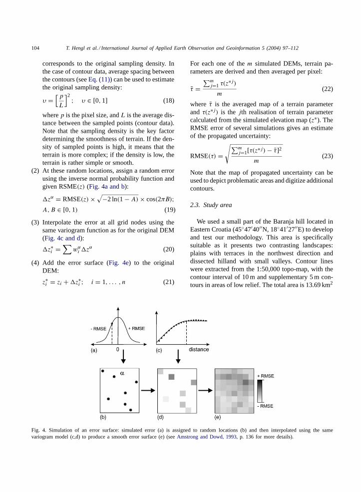
(2) At these random locations, assign a random errorusing the inverse normal probability function andgiven RSME(z) (Fig. 4a and b):

�zα = RMSE(z)×√−2 ln(1− A)× cos(2πB);

A,B ∈ [0,1) (19)

(3) Interpolate the error at all grid nodes using thesame variogram function as for the original DEM(Fig. 4c and d):

�z∗i =∑wαi �z

α (20)

(4) Add the error surface (Fig. 4e) to the originalDEM:

z∗i = zi +�z∗i ; i = 1, . . . , n (21)

Fig. 4. Simulation of an error surface: simulated error (a) is assigned to random locations (b) and then interpolated using the samevariogram model (c,d) to produce a smooth error surface (e) (seeAmstrong and Dowd, 1993, p. 136 for more details).

For each one of them simulated DEMs, terrain pa-rameters are derived and then averaged per pixel:

τ =∑mj=1 τ(z

∗j)m

(22)

where τ is the averaged map of a terrain parameterand τ(z∗j) is the jth realisation of terrain parametercalculated from the simulated elevation map (z∗). TheRMSE error of several simulations gives an estimateof the propagated uncertainty:

RMSE(τ) =√∑m

j=1[τ(z∗j)− τ]2m

(23)

Note that the map of propagated uncertainty can beused to depict problematic areas and digitize additionalcontours.

2.3. Study area

We used a small part of the Baranja hill located inEastern Croatia (45◦47′40′′N, 18◦41′27′′E) to developand test our methodology. This area is specificallysuitable as it presents two contrasting landscapes:plains with terraces in the northwest direction anddissected hilland with small valleys. Contour lineswere extracted from the 1:50,000 topo-map, with thecontour interval of 10 m and supplementary 5 m con-tours in areas of low relief. The total area is 13.69 km2


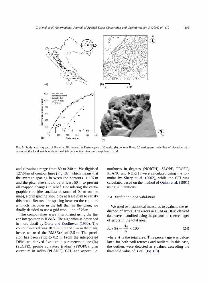
Fig. 5. Study area: (a) part of Baranja hill, located in Eastern part of Croatia; (b) contour lines; (c) variogram modelling of elevation withzoom on the local neighbourhood and (d) perspective view on interpolated DEM.

and elevations range from 80 to 240 m. We digitised127.6 km of contour lines (Fig. 5b), which means thatthe average spacing between the contours is 107 mand the pixel size should be at least 50 m to presentall mapped changes in relief. Considering the carto-graphic rule (the smallest distance of 0.4 m on themap), a grid spacing should be at least 20 m to satisfythis scale. Because the spacing between the contoursis much narrower in the hill than in the plain, wefinally decided to use a grid resolution of 25 m.

The contour lines were interpolated using the lin-ear interpolator inILWIS. The algorithm is describedin more detail byGorte and Koolhoven (1990). Thecontour interval was 10 m in hill and 5 m in the plain,hence we used the RMSE(z) of 2.5 m. The preci-sion has been setup to 0.2 m. From the interpolatedDEM, we derived five terrain parameters: slope (%)(SLOPE), profile curvature (rad/m) (PROFC), plancurvature in rad/m (PLANC), CTI, and aspect, i.e.

northness in degrees (NORTH). SLOPE, PROFC,PLANC and NORTH were calculated using the for-mulas by Shary et al. (2002), while the CTI wascalculated based on the method ofQuinn et al. (1991)using 20 iterations.

2.4. Evaluation and validation

We used two statistical measures to evaluate the re-duction of errors. The errors in DEM or DEM-deriveddata were quantified using the proportion (percentage)of errors in the total area:

Ae (%) = Ae

A× 100 (24)

whereA is the total area. This percentage was calcu-lated for both padi terraces and outliers. In this case,the outliers were detected ast-values exceeding thethreshold value of 3.219 (Eq. (6)).


To validate the effect of reduction of errors onsoil-landscape modelling, we used two applications.We first compared accuracy of classifying the land-forms for unfiltered and filtered data. This was doneby comparing an aerial photo-interpretation mapwith the results of supervised classifications(Hengland Rossiter, 2003). Second, we used a data setof 59 soil observations of thickness of the solum(SOLUM). This is the depth to parent material,in this case alluvial deposits and layers of loess.SOLUM was correlated with terrain parameters andmapped in the entire area. We observed the changein goodness of fit (R2) for the unfiltered and fil-tered data. Note that we did not evaluate effects ofthe grid size and vertical resolution on success ofsoil-landscape modelling. It seems that these are notthe real factors controlling the quality of terrain pa-rameters but should be inferred from the scale ofresearch and given data quality (RMSE(z) or contourinterval).

Fig. 6. Semi-automated DEM filtering: (a) automated detection of medial axes; (b) normal probability of finding the elevation value withinthe given neighbourhood (black pixels indicate probable outliers) and (c) change in elevation values (above) and reduction of padi terracesin percentage (below). See text for more explanation.

3. Results

3.1. Improving the DEM

A first interpolation of bulk contour data resultedin 17.3% of the total area being represented by paditerraces (Fig. 6c), most of them located in the plainregion (northwest corner). The automated extractionof medial axes detected hypothetical ridges and val-ley bottoms in 2.2% of the total area (Fig. 6a). Af-ter the second interpolation using added medial axes,the proportion of padi terraces was reduced to 4.5%(Fig. 6c, DEM L1–DEM L0). The biggest adjustmentof elevation was in the plain region. The reduction ofoutliers (DEM L2 - DEM L1) did not contribute to thereduction of padi terraces. Finally, the proportion ofthe padi terraces was reduced to 2.2% (Fig. 6c).

The variogram analysis of the contour lines gave anisotropic exponential model with no nugget and fairlystrong spatial dependence (Fig. 5candTable 1). Note


Table 1Variogram modelling of terrain parameters.

Terrain parametera Variogram modellingb

Unit AVG S.D. Model Anisotropy C0 C0 + C1 R R (10%)

DEM m 156.4 43.1 Exponential No 0 1350 675 1554SLOPE % 13.6 11.6 Exponential No 0 88 115 265PROFC rad m−1 0.00 0.17 Spherical Yes 0.006 0.0235 156 104PLANC rad m−1 −0.03 1.26 Spherical Yes 0.68 1.82 183 112CTI – 6.84 1.31 Exponential Yes 0.45 1.78 85 171NORTH – 90.0 47.0 Exponential Yes 0 2450 232 534

a AVG: mean value; S.D.: standard deviation.bC0: Nugget;C0 + C1: Sill; R: range parameter;R (10%): distance at which covariance reaches 10% of the sill.

in Fig. 5cthat probably the gaussian model would fitthe data better in the local neighbourhood (150 m).However, the data inspection showed that the expo-nential model fits the data in overall better. In thecase of the 3× 3 window environment, we calculatedweightswA = 0.253 andwB = −0.003. This meansthat this algorithm will give much higher importanceto the neighbours in the cardinal directions. For acomparison, the inverse distance interpolation wouldgive weightswA = 0.146 andwB = −0.104. For the5×5 window environment, the prediction of elevationis still done mainly from the closest neighbours. Theremaining weights (wC, wD, wE) accounted for only16.3% of the total cumulative weights (Table 1). Thismeans that, although the elevation values are corre-lated at long distances, there is not a large differencebetween using the 3× 3 and 5× 5 filters. Compari-son of the predicted and unfiltered values, showed thatthe difference is unbiased (δ = 0), while the standarddeviation (sδ = 1.28) was lower than the RMSE(z).The values with the lowest probability occurred at lo-cations where the density of contour lines was high-est, e.g. at steep slopes (Fig. 6b). This confirms thatthe filtering of outliers has a smoothing effect. Notethat the final change in elevation values, calculated asa difference between the old and adjusted elevationvalues does not exceed RMSE(z) (Fig. 6c).

The changes in the DEM are in general relativelysmall. The finally adjusted (DEM L3) does not dif-fer significantly from the original DEM in the cen-tral tendency measures (z = 157.2, sz = 43.8 versusz = 156.4, sz = 43.1). The histogram comparison,however, showed smoother distribution of values forDEM L3. For comparison, the unfilteredDEM L0 was

characterized by the typical grouping around the con-tour values (z = 90,100, . . . ). This difference corre-sponds to the results ofBrown and Bara (1994).

3.2. Errors in terrain parameters

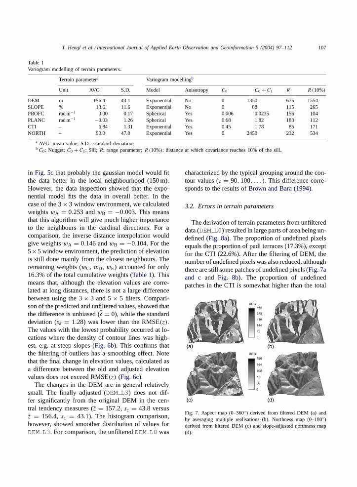
The derivation of terrain parameters from unfiltereddata (DEM L0) resulted in large parts of area being un-defined (Fig. 8a). The proportion of undefined pixelsequals the proportion of padi terraces (17.3%), exceptfor the CTI (22.6%). After the filtering of DEM, thenumber of undefined pixels was also reduced, althoughthere are still some patches of undefined pixels (Fig. 7aand c and Fig. 8b). The proportion of undefinedpatches in the CTI is somewhat higher than the total

Fig. 7. Aspect map (0–360◦) derived from filtered DEM (a) andby averaging multiple realisations (b). Northness map (0–180◦)derived from filtered DEM (c) and slope-adjusted northness map(d).


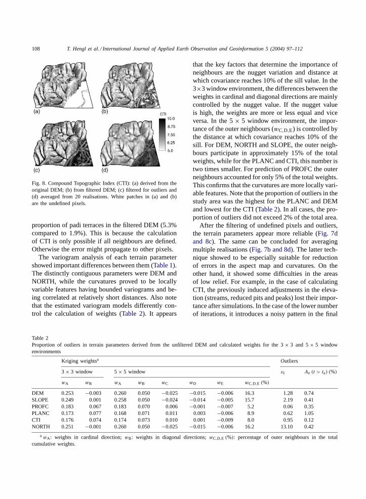
Fig. 8. Compound Topographic Index (CTI): (a) derived from theoriginal DEM; (b) from filtered DEM; (c) filtered for outliers and(d) averaged from 20 realisations. White patches in (a) and (b)are the undefined pixels.

proportion of padi terraces in the filtered DEM (5.3%compared to 1.9%). This is because the calculationof CTI is only possible if all neighbours are defined.Otherwise the error might propagate to other pixels.

The variogram analysis of each terrain parametershowed important differences between them (Table 1).The distinctly contiguous parameters were DEM andNORTH, while the curvatures proved to be locallyvariable features having bounded variograms and be-ing correlated at relatively short distances. Also notethat the estimated variogram models differently con-trol the calculation of weights (Table 2). It appears

Table 2Proportion of outliers in terrain parameters derived from the unfiltered DEM and calculated weights for the 3× 3 and 5× 5 windowenvironments

Kriging weightsa Outliers

3× 3 window 5× 5 window sδ Ae (t > ta) (%)

wA wB wA wB wC wD wE wC,D,E (%)

DEM 0.253 −0.003 0.260 0.050 −0.025 −0.015 −0.006 16.3 1.28 0.74SLOPE 0.249 0.001 0.258 0.050 −0.024 −0.014 −0.005 15.7 2.19 0.41PROFC 0.183 0.067 0.183 0.070 0.006 −0.001 −0.007 5.2 0.06 0.35PLANC 0.173 0.077 0.168 0.071 0.011 0.003 −0.006 8.9 0.62 1.05CTI 0.176 0.074 0.174 0.073 0.010 0.001 −0.009 8.0 0.95 0.12NORTH 0.251 −0.001 0.260 0.050 −0.025 −0.015 −0.006 16.2 13.10 0.42

awA: weights in cardinal direction;wB: weights in diagonal directions;wC,D,E (%): percentage of outer neighbours in the totalcumulative weights.

that the key factors that determine the importance ofneighbours are the nugget variation and distance atwhich covariance reaches 10% of the sill value. In the3×3 window environment, the differences between theweights in cardinal and diagonal directions are mainlycontrolled by the nugget value. If the nugget valueis high, the weights are more or less equal and viceversa. In the 5× 5 window environment, the impor-tance of the outer neighbours (wC,D,E) is controlled bythe distance at which covariance reaches 10% of thesill. For DEM, NORTH and SLOPE, the outer neigh-bours participate in approximately 15% of the totalweights, while for the PLANC and CTI, this number istwo times smaller. For prediction of PROFC the outerneighbours accounted for only 5% of the total weights.This confirms that the curvatures are more locally vari-able features. Note that the proportion of outliers in thestudy area was the highest for the PLANC and DEMand lowest for the CTI (Table 2). In all cases, the pro-portion of outliers did not exceed 2% of the total area.

After the filtering of undefined pixels and outliers,the terrain parameters appear more reliable (Fig. 7dand 8c). The same can be concluded for averagingmultiple realisations (Fig. 7b and 8d). The latter tech-nique showed to be especially suitable for reductionof errors in the aspect map and curvatures. On theother hand, it showed some difficulties in the areasof low relief. For example, in the case of calculatingCTI, the previously induced adjustments in the eleva-tion (streams, reduced pits and peaks) lost their impor-tance after simulations. In the case of the lower numberof iterations, it introduces a noisy pattern in the final


Fig. 9. Comparison of PLANC calculated using a single, 20 and 50 realisations. See alsohttp://www.itc.nl/personal/shrestha/DTA/foranimated display of reduction of errors.

derivative, which does not necessarily reflect the realcase. There is certainly a difference in mapping CTIin plain when averaging multiple realisations and fil-tering slopes (Fig. 7c and 8d). The key reason for thisdifference is estimation of slope in the plain area. Aver-aging multiple realisations in general increases slopesin the plain region (under-estimation of CTI). The fil-tering of slope map, on the other hand, maintains fairlysmall values (over-estimation of CTI). In this case, theover-estimation of CTI appears to be more realistic asit portrays the watershed as being connected.

In other examples, averaging multiple realisa-tions seems to be the most robust way of producing

Fig. 10. Landform classification: (a) the reference aerial photo-interpretation map with the legend; (b) results of classification usingunfiltered terrain parameters and (c) after the filtering of terrain parameters.

smoother terrain parameters, with much less artefactsand more natural appearance. TheFig. 9 shows, forexample, difference between PLANC calculated usinga single, 20 and 50 realisations. The improvement isvisible even after few realisations. After higher num-ber of iterations, PLANC shows connected, smootherfeatures; also note that the artefacts in the plain regiondisappeared from the map.

3.3. Effects on soil-landscape modelling

Comparison of landform classification usingunfiltered and filtered terrain parameters showed



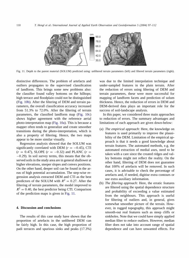
Fig. 11. Depth to the parent material (SOLUM) predicted using: unfiltered terrain parameters (left) and filtered terrain parameters (right).

distinctive differences. The problem of artefacts andoutliers propagates to the supervised classificationof landform. This brings some new problems also:the classifier found valley bottoms on the hilltops;high terrace and floodplain could not be distinguished(Fig. 10b). After the filtering of DEM and terrain pa-rameters, the overall classification accuracy increasedfrom 51.3% to 72.0%. After the filtering of terrainparameters, the classified landform map (Fig. 10c)shows higher agreement with the reference aerialphoto-interpretation map (Fig. 10a). This is because amapper often tends to generalize and create smoothertransitions during the photo-interpretation, which isalso a property of filtering. Hence, the two mapsappear to be more similar visually.

Regression analysis showed that the SOLUM wassignificantly correlated with DEM (r = −0.45), CTI(r = 0.47), SLOPE (r = −0.32) and PLANC (r =−0.29). In soil survey terms, this means that the ob-served soils in the study area are in general shallower athigher elevations, steeper slopes and convex positions.On the other hand, deeper soil can be found in the ar-eas of high potential accumulation. The step-wise re-gression analysis extracted DEM and CTI as the bestpredictors of the SOLUM withR2 = 0.27. After thefiltering of terrain parameters, the model improved toR2 = 0.40, the best predictor being CTI. Comparisonof the prediction maps is given inFig. 11.

4. Discussion and conclusions

The results of this case study have shown that theproportion of artefacts in the unfiltered DEM canbe fairly high. In this case, the high proportion ofpadi terraces and spurious sinks and peaks (17.3%)

was due to the limited interpolation technique andunder-sampled features in the plain terrain. Afterthe reduction of errors using filtering of DEM andterrain parameters, these were more successful formapping of landform facets and prediction of solumthickness. Hence, the reduction of errors in DEM andDEM-derived data plays an important role for thesuccess of soil-landscape analysis.

In this paper, we considered three main approachesto reduction of errors. The summary advantages andlimitations of each approach are given down-below:

(a) The empirical approach: Here, the knowledge onfeatures is used primarily to improve the plausi-bility of the DEM. Limitation of the empirical ap-proach is that it needs a good knowledge aboutterrain features. The automated methods, e.g. theautomated extraction of medial axes, need to betaken with a care since the created ridges and val-ley bottoms might not reflect the reality. On theother hand, filtering of DEM does not guaranteethat 100% of artefacts will be removed. In suchcases, it is advisable to check the percentage ofartefacts and, if needed, digitise extra contours oruse extra auxiliary information.

(b) The filtering approach: Here, the erratic featuresare filtered using the spatial dependence structureand probability of exceeding a value estimatedfrom the neighbours. This approach is usefulfor filtering of outliers and, in general, givessomewhat smoother picture of the terrain. How-ever, in rugged topography, this approach mightsmooth-out real features such as steep cliffs orsinkholes. Note that we could have simply appliedmedian filter to reduce outliers. However, medianfilter does not take into account range of spatialdependence and can have unwanted effects. For


example, if the elevation is strongly correlatedspatially and at longer distances, then the confi-dence limits need to be much narrower. Similarly,if the elevations vary at small distances, than thedefinition of an outlier is not as strict. These as-pects cannot be incorporated into a simple medialfiltering. The problem with the geostatistical anal-ysis is that the variogram models for terrain pa-rameters and threshold distances are assumed cor-rect, although they can differ greatly for differentparts of the area as well as for different grid sizes.It may therefore be more reasonable to use empir-ical or field-validated models of spatial variationand threshold limits or estimate the true values ofterrain parameters using transect studies. Anotherproblem with this approach is the selection of thefiltering window size. It appears that the 3×3 win-dow environment is large enough for filtering ofcurvatures and CTI (i.e. locally varying features).Larger window sizes are computationally moredemanding, but more accurate. Also note that be-cause we are only interested in the local spatialdependence, only first 10–15 surrounding pixelsneed to be considered for variogram modelling.

(c) The simulation approach: This approach isbased on geostatistical simulations and is fullydata-driven. The errors are reduced by calculatingthe average value of terrain parameter calculatedfrom multiple equiprobable realisations of DEM.This in general creates more natural and morecontiguous picture of the geomorphology. The ad-vantage of averaging multiple realisations is thatit does not need calculation of filtering weightsor selection of the window size. It is especiallyinteresting as it can be fully automated. It is alsoattractive because it offers a (propagated) measureof the uncertainty of deriving a terrain parameter.The possible problems with error propagation, isthat it can be time-consuming, as it often needsmany realisations. It also needs a good estimateof the error in input values (RMSE(z)). For oursample area we have evaluated that the used inputfor the error propagation was too high in the plainregion. This had an effect of increasing the slope(and CTI) in the plain. If you compare this resultsto the results ofHolmes et al. (2000), you willnotice that our simulated error is much smootherthan if we would use conditional simulations

(geostatistical simulations often introduce noiseas addition to the continuous error surface). Webelieve that even simulated topography needs tobe as smooth as the input DEM, i.e.it should notshow noisy pattern. This means that one needsto use variogram models with zero nugget andslightly asymptotical towards the 0-nugget (likegaussian or bessel model) in geostatistical simula-tions. Otherwise, simulations will only introduceroughness that does not reflect true topography.At least not at the given mapping scale.

Finally, one should keep in mind that elevation, i.e. to-pography is a non-stationary and non-periodic feature.Therefore, it is probably more advisable to estimatespatial variation of topography at local and not globalscales. Especially in karst and heavily dissected areas,it will be hard to estimate the global model of spatialvariation, which typically means that filtering mightover-smooth some untypical but important geomor-phic features such as cockpits, cliffs, embankments orreal padi terraces. It cannot be excluded, that even inour sample area we have incidentally corrected awaysome small number of real features such as real ter-races and depressions that can occur naturally. Onesolution to this problem is to cut or mask out areasthat make no sense for the terrain analysis, e.g. realrice terraces or escarpments.

References

Addink, E., Stein, A., 1999. A comparison of conventionaland geostatistical methods to replace clouded pixels inNOAA-AVHRR images. Int. J. Rem. Sens. 20 (5), 961–977.

Amstrong, M., Dowd, P.A. (Eds.), 1993. Geostatistical Simulations,vol. 7, Proceedings of the Geostatistical Simulation Workshop,Fontainebleau, France, 27–28 May. Kluwer AcademicPublishers, Dodrecht.

Banks, J. (Ed.), 1998. Handbook of Simulation—Principles,Methodology, Advances, Applications, and Practice. Wiley,New York.

Beers, T.W., Dress, P.E., Wensel, L.C., 1966. Aspect transformationin site productivity research. J. For. 64, 691–692.

Brown, D., Bara, T., 1994. Recognition and reduction of systematicerror in elevation and derivative surfaces from 7.5-minuteDEMs. Photogr. Eng. Rem. Sens. 60 (2), 189–194.

Burrough, P., McDonnell, R., 1998. Principles of GeographicalInformation Systems. Oxford University Press, Oxford.

Burrough, P., van Gaans, P., MacMillan, R., 2000. High-resolutionlandform classification using fuzzyk-means. Fuzzy Sets Syst.113, 37–52.


Dakowicz, M., Gold, C.M., 2002. Extracting meaningfulslopes from terrain contours. In: Sloot, P.M.A., Tan,C.J.K., Dongarra, J.J., Hoekstra, A.G. (Eds.), ComputationalScience—ICCS 2002. Lecture Notes in Computer Science,vol. 2331. Springer-Verlag, Berlin, Heidelberg, Amsterdam,pp. 144–153.

Evans, I., Cox, N., 1999. Relations between land surfaceproperties: altitude, slope and cruvature. In: Hergarten, S.,Neugebauer, H. (Eds.), Process Modelling and LandformEvolution. Springer-Verlag, Berlin, pp. 13–45.

Felicisimo, A., 1994. Parametric statistical method for errordetection in digital elevation models. ISPRS J. Photogr. Rem.Sens. 49 (4), 29–33.

Florinsky, I., 1998. Accuracy of local topographic variables derivedfrom digital elevation models. Int. J. Geogr. Inform. Sci. 12 (1),47–62.

Gessler, P., Moore, I., McKenzie, N., Ryan, P., 1995. Soil-landscapemodelling and spatial prediction of soil attributes. Int. J. Geogr.Inform. Syst. 9 (4), 421–432.

Gorte, B., Koolhoven, W., 1990. Interpolation between isolinesbased on the Borgefors distance transform. ITC J. 1 (3), 245–247.

Hengl, T., Rossiter, D.G., 2003. Supervised landform classificationto enhance and replace photo-interpretation in semi-detailedsoil survey. Soil Sci. Soc. Am. J. 67 (5), 1810–1822.

Hengl, T., Gruber, S., Shrestha, D., 2003. Digital TerrainAnalysis in ILWIS. Lecture notes, International Institute forGeo-Information Science & Earth Observation (ITC), Enschede,URL: http://www.itc.nl/personal/shrestha/DTA/.

Heuvelink, G., 1998. Error Propagation in EnvironmentalModelling with GIS. Taylor & Francis, London, UK.

Holmes, K., Chadwick, O., Kyriakidis, P., 2000. Error in a USGS30 m digital elevation model and its impact on digital terrainmodeling. J. Hydrol. 233, 154–173.

Hutchinson, M., 1989. A new procedure for gridding elevationand stream line data with automatic removal of spurious pits.J. Hydrol. 106, 211–232.

Isaaks, E., Srivastava, R., 1989. Applied Geostatistics. OxfordUniversity Press, New York.

Li, Z., 1994. A comparative study of the accuracy of digitalterrain models (DTMs) based on various data models. ISPRSJ. Photogr. Rem. Sens. 49, 2–11.

Lopez, C., 2000. Improving the elevation accuracy of digitalelevation models: a comparison of some error detectionprocedures. Trans. GIS 4 (1), 43–64.

MacMillan, R., Pettapiece, W., Nolan, S., Goddard, T., 2000. Ageneric procedure for automatically segmenting landforms intolandform elements using DEMs, heuristic rules and fuzzy logic.Fuzzy Sets Syst. 113, 81–109.

Martinoni, D., 2002. Models and experiments for quality handlingin digital terrain modelling. Ph.D. thesis, University of Zurich.

McKenzie, N., Ryan, P., 1999. Spatial prediction of soil propertiesusing environmental correlation. Geoderma 89 (1–2), 67–94.

McKenzie, N., Gessler, P., Ryan, P., O’Connell, D., 2000. The roleof terrain analysis in soil mapping. In: Wilson, J.P., Gallant, J.C.(Eds.), Terrain Analysis: Principles and Applications. Wiley,Inc., pp. 245–265.

Moore, I., Gessler, P., Nielsen, G., Peterson, G., 1993. Soil attributeprediction using terrain analysis. Soil Sci. Soc. Am. J. 57 (2),443–452.

Pilouk, M., Tempfli, K., 1992. A digital image processing approachto creating DTMs from digitized contours. Int. Arch. Photogr.Rem. Sens. 29 (B4), 956–961.

Quinn, P., Beven, K., Chevallier, P., Planchon, O., 1991. Theprediction of hillslope flow paths for distributed hydrologicalmodelling using digital terrain models. Hydrol. Processes 5,59–79.

Raaflaub, L., Collins, M., 2002. The effect errors in griddeddigital elevation have on derived topographic parametersusing Monte Carlo simulation: a comparison of algorithms.In: Hunter, G.J., Lowell, K. (Eds.), Proceedings of the 5thInternational Symposium on Spatial Accuracy Assesment inNatural Resources and Environmental Sciences (Accuracy2002), RMIT University, Melbourne, Australia, p. 279.

Schneider, B., 1998. Geomorphologically plausibel reconstructionof the digital representation of terrain surfaces from contourdata (in German). Ph.D. thesis, Universtiy of Zurich.

Shary, P., Sharaya, L., Mitusov, A., 2002. Fundamental quantitativemethods of land surface analysis. Geoderma 107 (1–2), 1–32.

Tang, G., Shi, W., Zhao, M., 2002. Evaluation on the accuracyof hydrologic data derived from DEMs of different spatialresolution. In: Hunter, G.J., Lowell, K. (Eds.), Proceedingsof the 5th International Symposium on Spatial AccuracyAssesment in Natural Resources and Environmental Sciences(Accuracy 2002), RMIT University, Melbourne, Australia,pp. 204–213.

Tempfli, K., 1999. DTM accuracy assesment. In: ASPRS AnnualConference, Portland, pp. 1–11.

Thompson, J., Bell, J., Butler, C., 2000. Digital elevationmodel resolution: effects on terrain attribute calculation andquantitative soil-landscape modeling. Geoderma 100, 67–89.

Wilson, J., Repetto, P., Snyder, R., 2000. Effect of data source, gridresolution, and flow-routing method on computed topographicattributes. In: Wilson, J.P., Gallant, J.C. (Eds.), Terrain Analysis:Principles and Applications. Wiley, New York, pp. 133–161.

Wise, S., 2000. Assessing the quality for hyrdological applicationsof digital elevation models derived from contours. Hydrol.Processes 14 (11–12), 1909–1929.


reduction of errors in digital terrain parameters used in soil-landscape modelling

Documents