recovering the spatial layout of cluttered...
TRANSCRIPT
Recovering the Spatial Layout of Cluttered Rooms
Varsha HedauElectical and Computer Engg. DepartmentUniversity of Illinois at Urbana Champaign
Derek Hoiem, David ForsythComputer Science Department
University of Illinois at Urbana Champaign{dhoiem,daf}@uiuc.edu
Abstract
In this paper, we consider the problem of recovering thespatial layout of indoor scenes from monocular images. Thepresence of clutter is a major problem for existing single-view 3D reconstruction algorithms, most of which rely onfinding the ground-wall boundary. In most rooms, thisboundary is partially or entirely occluded. We gain robust-ness to clutter by modeling the global room space with aparameteric 3D “box” and by iteratively localizing clutterand refitting the box. To fit the box, we introduce a struc-tured learning algorithm that chooses the set of parametersto minimize error, based on global perspective cues. Ona dataset of 308 images, we demonstrate the ability of ouralgorithm to recover spatial layout in cluttered rooms andshow several examples of estimated free space.
1. IntroductionLook at the image in Fig. 1. From this single image,
we humans can immediately grasp the spatial layout of thescene. Our understanding is not restricted to the immedi-ately visible portions of the chairs, sofa, and walls, but alsoincludes some estimate of the entire space. We want to pro-vide the same spatial understanding to computers. Doingso will allow more precise reasoning about free space (e.g.,where can I walk) and improved object reasoning. In thispaper, we focus on indoor scenes because they require care-ful spatial reasoning and are full of object clutter making thespatial layout estimation difficult for existing algorithms.
Recovering Spatial Layout. To recover the spatial lay-out of an image, we first need to answer: how shouldwe parameterize the scene space? Existing parametriza-tions include: a predefined set of prototype global scenegeometries [17]; a gist [18] of a scene describing its spa-tial characteristics; a 3D box [11, 23] or collection of 3Dpolyhedrals [6, 15, 19]; boundaries between ground andwalls [1, 4]; depth-ordered planes [26]; constrained ar-rangements of corners [13]; a pixel labeling of approximatelocal surface orientations [9], possibly with ordering con-straints [14]; or depth estimates at each pixel [22]. Models
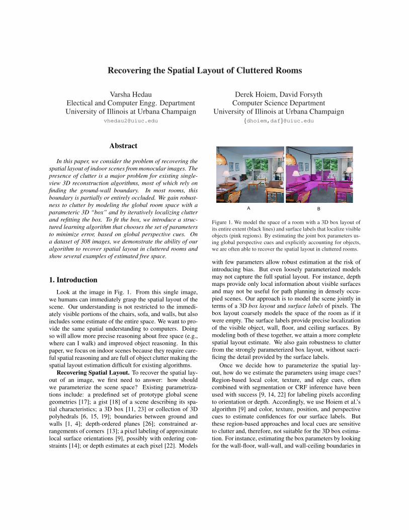
Figure 1. We model the space of a room with a 3D box layout ofits entire extent (black lines) and surface labels that localize visibleobjects (pink regions). By estimating the joint box parameters us-ing global perspective cues and explicitly accounting for objects,we are often able to recover the spatial layout in cluttered rooms.
with few parameters allow robust estimation at the risk ofintroducing bias. But even loosely parameterized modelsmay not capture the full spatial layout. For instance, depthmaps provide only local information about visible surfacesand may not be useful for path planning in densely occu-pied scenes. Our approach is to model the scene jointly interms of a 3D box layout and surface labels of pixels. Thebox layout coarsely models the space of the room as if itwere empty. The surface labels provide precise localizationof the visible object, wall, floor, and ceiling surfaces. Bymodeling both of these together, we attain a more completespatial layout estimate. We also gain robustness to clutterfrom the strongly parameterized box layout, without sacri-ficing the detail provided by the surface labels.
Once we decide how to parameterize the spatial lay-out, how do we estimate the parameters using image cues?Region-based local color, texture, and edge cues, oftencombined with segmentation or CRF inference have beenused with success [9, 14, 22] for labeling pixels accordingto orientation or depth. Accordingly, we use Hoiem et al.’salgorithm [9] and color, texture, position, and perspectivecues to estimate confidences for our surface labels. Butthese region-based approaches and local cues are sensitiveto clutter and, therefore, not suitable for the 3D box estima-tion. For instance, estimating the box parameters by lookingfor the wall-floor, wall-wall, and wall-ceiling boundaries in
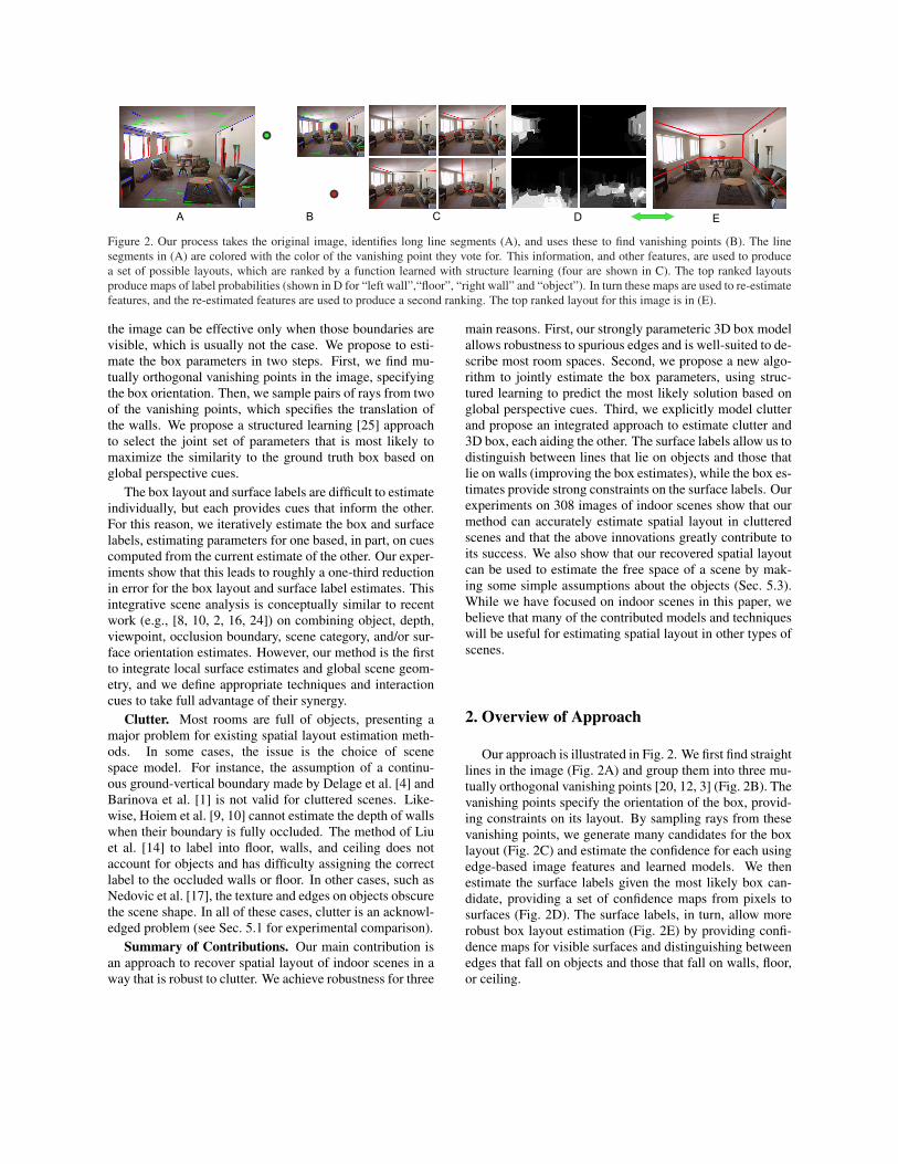
Figure 2. Our process takes the original image, identifies long line segments (A), and uses these to find vanishing points (B). The linesegments in (A) are colored with the color of the vanishing point they vote for. This information, and other features, are used to producea set of possible layouts, which are ranked by a function learned with structure learning (four are shown in C). The top ranked layoutsproduce maps of label probabilities (shown in D for “left wall”,“floor”, “right wall” and “object”). In turn these maps are used to re-estimatefeatures, and the re-estimated features are used to produce a second ranking. The top ranked layout for this image is in (E).
the image can be effective only when those boundaries arevisible, which is usually not the case. We propose to esti-mate the box parameters in two steps. First, we find mu-tually orthogonal vanishing points in the image, specifyingthe box orientation. Then, we sample pairs of rays from twoof the vanishing points, which specifies the translation ofthe walls. We propose a structured learning [25] approachto select the joint set of parameters that is most likely tomaximize the similarity to the ground truth box based onglobal perspective cues.
The box layout and surface labels are difficult to estimateindividually, but each provides cues that inform the other.For this reason, we iteratively estimate the box and surfacelabels, estimating parameters for one based, in part, on cuescomputed from the current estimate of the other. Our exper-iments show that this leads to roughly a one-third reductionin error for the box layout and surface label estimates. Thisintegrative scene analysis is conceptually similar to recentwork (e.g., [8, 10, 2, 16, 24]) on combining object, depth,viewpoint, occlusion boundary, scene category, and/or sur-face orientation estimates. However, our method is the firstto integrate local surface estimates and global scene geom-etry, and we define appropriate techniques and interactioncues to take full advantage of their synergy.
Clutter. Most rooms are full of objects, presenting amajor problem for existing spatial layout estimation meth-ods. In some cases, the issue is the choice of scenespace model. For instance, the assumption of a continu-ous ground-vertical boundary made by Delage et al. [4] andBarinova et al. [1] is not valid for cluttered scenes. Like-wise, Hoiem et al. [9, 10] cannot estimate the depth of wallswhen their boundary is fully occluded. The method of Liuet al. [14] to label into floor, walls, and ceiling does notaccount for objects and has difficulty assigning the correctlabel to the occluded walls or floor. In other cases, such asNedovic et al. [17], the texture and edges on objects obscurethe scene shape. In all of these cases, clutter is an acknowl-edged problem (see Sec. 5.1 for experimental comparison).
Summary of Contributions. Our main contribution isan approach to recover spatial layout of indoor scenes in away that is robust to clutter. We achieve robustness for three
main reasons. First, our strongly parameteric 3D box modelallows robustness to spurious edges and is well-suited to de-scribe most room spaces. Second, we propose a new algo-rithm to jointly estimate the box parameters, using struc-tured learning to predict the most likely solution based onglobal perspective cues. Third, we explicitly model clutterand propose an integrated approach to estimate clutter and3D box, each aiding the other. The surface labels allow us todistinguish between lines that lie on objects and those thatlie on walls (improving the box estimates), while the box es-timates provide strong constraints on the surface labels. Ourexperiments on 308 images of indoor scenes show that ourmethod can accurately estimate spatial layout in clutteredscenes and that the above innovations greatly contribute toits success. We also show that our recovered spatial layoutcan be used to estimate the free space of a scene by mak-ing some simple assumptions about the objects (Sec. 5.3).While we have focused on indoor scenes in this paper, webelieve that many of the contributed models and techniqueswill be useful for estimating spatial layout in other types ofscenes.
2. Overview of Approach
Our approach is illustrated in Fig. 2. We first find straightlines in the image (Fig. 2A) and group them into three mu-tually orthogonal vanishing points [20, 12, 3] (Fig. 2B). Thevanishing points specify the orientation of the box, provid-ing constraints on its layout. By sampling rays from thesevanishing points, we generate many candidates for the boxlayout (Fig. 2C) and estimate the confidence for each usingedge-based image features and learned models. We thenestimate the surface labels given the most likely box can-didate, providing a set of confidence maps from pixels tosurfaces (Fig. 2D). The surface labels, in turn, allow morerobust box layout estimation (Fig. 2E) by providing confi-dence maps for visible surfaces and distinguishing betweenedges that fall on objects and those that fall on walls, floor,or ceiling.
(a) (b)
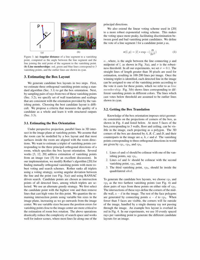
Figure 3. (a) Angular distance of a line segment to a vanishingpoint, computed as the angle between the line segment and theline joining the mid point of the segment to the vanishing point.(b) Line memberships: red, green and blue lines correspond to 3vanishing points, and the outlier lines are shown in cyan.
3. Estimating the Box Layout
We generate candidate box layouts in two steps. First,we estimate three orthogonal vanishing points using a stan-dard algorithm (Sec. 3.1) to get the box orientation. Next,by sampling pairs of rays from two of these vanishing points(Sec. 3.2), we specify set of wall translations and scalingsthat are consistent with the orientation provided by the van-ishing points. Choosing the best candidate layout is diffi-cult. We propose a criteria that measures the quality of acandidate as a whole and learn it with structured outputs(Sec. 3.3).
3.1. Estimating the Box Orientation
Under perspective projection, parallel lines in 3D inter-sect in the image plane at vanishing points. We assume thatthe room can be modelled by a box layout and that mostsurfaces inside the room are aligned with the room direc-tions. We want to estimate a triplet of vanishing points cor-responding to the three principal orthogonal directions of aroom, which specifies the box layout orientation. Severalworks [3, 12, 20] address estimation of vanishing pointsfrom an image (see [5] for an excellent discussion). Inour implementation, we modify Rother’s algorithm [20] forfinding mutually orthogonal vanishing points with more ro-bust voting and search schemes. Rother ranks all tripletsusing a voting strategy, scoring angular deviation betweenthe line and the point (see Fig. 3(a)) and using RANSACdriven search. Candidate points are chosen as intersectionpoints of all detected lines, among which triplets are se-lected. We use an alternate greedy strategy. We first selectthe candidate point with the highest vote and then removelines that cast high votes for this point. We quantize the re-maining intersection points using variable bin sizes in theimage plane, increasing as we go outwards from the imagecenter. We use variable sizes because the position errors forvanishing point close to the image center are more critical tothe estimation of room box rotation. The above operationsdrastically reduce the complexity of search space and workswell for indoor scenes, where most lines lie along one of the
principal directions.We also extend the linear voting scheme used in [20]
to a more robust exponential voting scheme. This makesthe voting space more peaky, facilitating discrimination be-tween good and bad vanishing point candidates. We definethe vote of a line segment l for a candidate point p as,
v(l, p) = |l| ∗ exp−(α
2σ2) (1)
α , where, is the angle between the line connecting p andmidpoint of l, as shown in Fig. 3(a), and σ is the robust-ness threshold. In all our experiments, we set σ = 0.1. Thestraight lines of length greater than 30 pixels are used forestimation, resulting in 100-200 lines per image. Once thewinning triplet is identified, each detected line in the imagecan be assigned to one of the vanishing points according tothe vote it casts for these points, which we refer to as linemembership. Fig. 3(b) shows lines corresponding to dif-ferent vanishing points in different colors. The lines whichcast votes below threshold are assumed to be outlier linesshown in cyan.
3.2. Getting the Box Translation
Knowledge of the box orientation imposes strict geomet-ric constraints on the projections of corners of the box, asshown in Fig. 4 and listed below. At most 5 faces of thebox,corresponding to 3 walls, floor and ceiling, can be vis-ible in the image, each projecting as a polygon. The 3Dcorners of the box are denoted by A, B, C, and D, and theircounterparts in the image are a, b, c and d. The vanishingpoints corresponding to three orthogonal directions in worldare given by vp1, vp2, and vp3.
1. Lines ab and cd should be colinear with one of the van-ishing points, say vp1,
2. Lines ad and bc should be colinear with the secondvanishing point, vp2, and,
3. The third vanishing point, vp3, should lie inside thequadrilateral abcd.
To generate the candidate box layouts, we choose vp1 andvp2 as the two farthest vanishing points (see Fig. 4) anddraw pairs of rays from these points on either side of vp3.The intersections of these rays define the corners of the mid-dle wall, a − d in the image. The rest of the face polygonsare generated by connecting points a − d to vp3. Whenfewer than 5 faces are visible, the corners will lie outsideof the image, handled by a single dummy ray not passingthrough the image. An example box layout is overlaid inred in Fig. 4. In our experiments, we use 10 evenly spacedrays per vanishing point to generate the different candidatelayouts for an image.
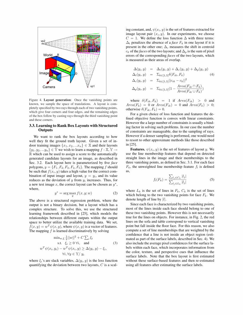
Figure 4. Layout generation: Once the vanishing points areknown, we sample the space of translations. A layout is com-pletely specified by two rays through each of two vanishing points,which give four corners and four edges, and the remaining edgesof the box follow by casting rays through the third vanishing pointand these corners.
3.3. Learning to Rank Box Layouts with StructuredOutputs
We want to rank the box layouts according to howwell they fit the ground truth layout. Given a set of in-door training images {x1, x2, ...xn} ∈ X and their layouts{y1, y2, ...yn} ∈ Y we wish to learn a mapping f : X, Y →R which can be used to assign a score to the automaticallygenerated candidate layouts for an image, as described inSec. 3.2. Each layout here is parameterized by five facepolygons, y = {F1, F2, F3, F4, F5}. The mapping f shouldbe such that f(xi, y) takes a high value for the correct com-bination of input image and layout, y = yi, and its valuereduces as the deviation of y from yi increases. Thus, fora new test image x, the correct layout can be chosen as y∗,where,
y∗ = arg maxy
f(x, y; w) (2)
The above is a structured regression problem, where theoutput is not a binary decision, but a layout which has acomplex structure. To solve this, we use the structuredlearning framework described in [25], which models therelationships between different outputs within the outputspace to better utilize the available training data. We set,f(x, y) = wT ψ(x, y), where ψ(x, y) is a vector of features.The mapping f is learned discriminatively by solving
minw,ξ12 ||w||2 + C
∑i ξi
s.t. ξi ≥ 0 ∀i, and (3)wT ψ(xi, yi) − wT ψ(xi, y) ≥ Δ(yi, y) − ξi,
∀i,∀y ∈ Y/ yi
where ξi’s are slack variables, Δ(yi, y) is the loss functionquantifying the deviation between two layouts, C is a scal-
ing constant, and, ψ(xi, y) is the set of features extracted forimage layout pair (xi, y). In our experiments, we chooseC = 1. We define the loss function Δ with three terms:Δt penalizes the absence of a face Fk in one layout if it ispresent in the other one; Δc measures the shift in centroidck of the faces of the two layouts; and Δp is the sum of pixelerrors of the corresponding faces of the two layouts, whichis measured as their areas of overlap.
Δ(yi, y) = Δt(yi, y) + Δc(yi, y) + Δp(yi, y)Δt(yi, y) = Σk∈[1,5]δ(Fik, Fk) (4)
Δc(yi, y) = Σk∈[1,5]||cik − ck||2
Δp(yi, y) = Σk∈[1,5](1 − Area(Fik ∩ Fk)Area(Fik ∪ Fk)
)
where δ(Fik, Fk) = 1 if Area(Fik) > 0 andArea(Fk) = 0 or Area(Fik) = 0 and Area(Fk) > 0;otherwise δ(Fik, Fk) = 0.
For a given choice of loss function and features the de-fined objective function is convex with linear constraints.However the a large number of constraints is usually a bind-ing factor in solving such problems. In our case the numberof constraints are manageable, due to the sampling of rays.However if a denser sampling is performed, one would needto resort to other approximate methods like those describedin [25].
Features. ψ(xi, y) is the set of features of layout y. Weuse the line membership features that depend on detectedstraight lines in the image and their memberships to thethree vanishing points, as defined in Sec. 3.1. For each faceFk, the unweighted line membership feature fl is definedas,
fl(Fk) =
∑lj∈Ck
|lj |∑
lj∈Lk|lj | (5)
where Lk is the set of lines in Fk, Ck is the set of lineswhich belong to the two vanishing points for face Fk. Wedenote length of line by |l|.
Since each face is characterized by two vanishing points,most of the lines inside each face should belong to one ofthese two vanishing points. However this is not necessarilytrue for the lines on objects. For instance, in Fig. 2, the redlines on the sofa and table correspond to vertical vanishingpoint but fall inside the floor face. For this reason, we alsocompute a set of line memberships that are weighted by theconfidence that a line is not inside an object region (esti-mated as part of the surface labels, described in Sec. 4). Wealso include the average pixel confidences for the surface la-bels within each face, which incorporates information fromthe color, texture, and perspective cues that influence thesurface labels. Note that the box layout is first estimatedwithout these surface-based features and then re-estimatedusing all features after estimating the surface labels.
4. Estimating Surface Labels
It is difficult to fit the box layout to general pictures ofrooms because “clutter”, such as tables, chairs, and sofas,obscures the boundaries between faces. Some of the fea-tures we use to identify the box may actually lie on thisclutter, which may make the box estimate less accurate. Ifwe have an estimate of where the clutter is, we should beable to get a more accurate box layout. Similarly, if wehave a good box layout estimate, we know the position ofits faces, which should allow us to better localize the clutter.
To estimate our surface labels, we use a modified versionof Hoiem et al.’s surface layout algorithm [9]. The image isoversegmented into superpixels, which are then partitionedinto multiple segmentations. Using color, texture, edge,and vanishing point cues computed over each segment, aboosted decision tree classifier estimates the likelihood thateach segment is valid (contains only one type of label) andthe likelihood of each possible label. These likelihoods arethen integrated pixel-wise over the segmentations to providelabel confidences for each superpixel. We modify the algo-rithm to estimate our floor, left/middle/right wall, ceiling,and object labels and add features from our box layout. Asbox layout features, we use the percentage area of a segmentoccupied by each face and the entropy of these overlaps,which especially helps to reduce confusion among the non-object room surfaces. In training, we use cross-validationto compute the box layout cues for the training set.
5. Experiments and Results
All experiments are performed on a dataset of 308 in-door images collected from the web and from LabelMe[21]. Images include a wide variety of rooms including, liv-ing rooms, bed rooms, corridors etc (see Fig. 6). We labelthese images into ground truth box layout faces: polygonboundaries of floor, left wall, middle wall, right wall, andceiling. We also label ground truth surface labels: segmen-tation masks for object, left, middle, and right wall, ceiling,and floor regions. We randomly split the dataset into a train-ing set of 204 and test set of 104 images.
We first evaluate the accuracy of our box layout and sur-face label estimates (Sec. 5.1). Our results indicate thatwe can recover layouts in cluttered rooms, that the integra-tion of surface labels and box layout is helpful, and thatour method compares favorably to existing methods. InSec. 5.2, we then analyze the contribution of errors by van-ishing point estimation and ray sampling in estimating boxtranslation. Finally, we show several qualitative results forfree space estimation in Sec. 5.3.
5.1. Evaluation of spatial layouts
We show several qualitative results in Fig. 6, and reportour quantitative results in Tables 1, 2 and 3.
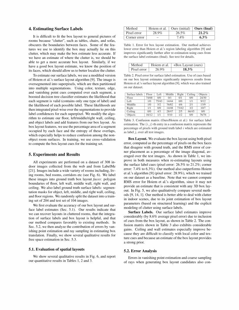
Method Hoiem et al. Ours (initial) Ours (final)Pixel error 28.9% 26.5% 21.2%Corner error – 7.4% 6.3%
Table 1. Error for box layout estimation. Our method achieveslower error than Hoiem et al.’s region labeling algorithm [9] andimproves significantly further after re-estimation using cues fromthe surface label estimates (final). See text for details.
Method Hoiem et al. +Box Layout (ours)Pixel error 26.9% 18.3%
Table 2. Pixel error for surface label estimation. Use of cues basedon our box layout estimates significantly improves results fromHoiem et al.’s surface layout algorithm [9], which was also trainedon our dataset.
Surface labels Floor Left Middle Right Ceiling ObjectsFloor 74/68 0/0 0/1 0/1 0/0 24/30Left 1/0 75/43 14/44 0/0 1/1 9/12Middlle 1/0 5/2 76/82 4/6 2/1 13/9Right 1/1 0/0 14/48 73/42 3/2 10/7Ceiling 0/0 4/3 28/47 2/5 66/45 0/0Objects 16/12 1/1 5/10 1/2 0/0 76/76
Table 3. Confusion matrix (Ours/Hoiem et al.) for surface labelestimation. The (i, j)-th entry in a confusion matrix represents thepercentage of pixels with ground truth label i which are estimatedas label j, over all test images.
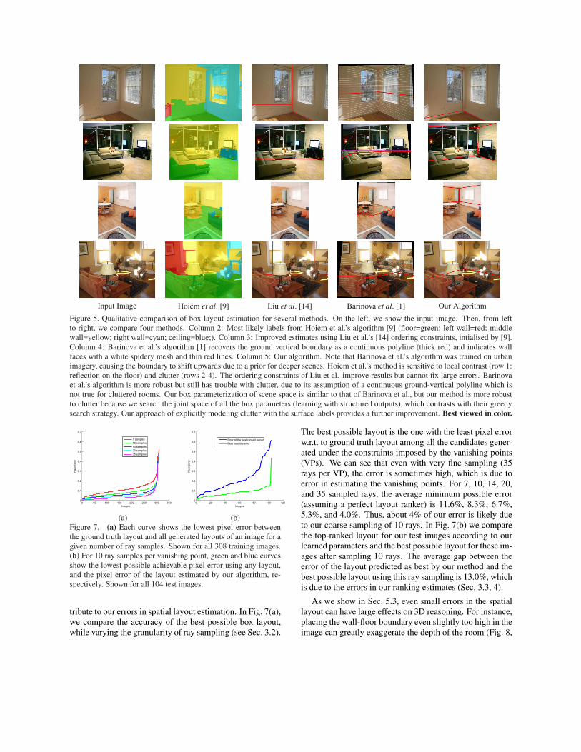
Box Layout. We evaluate the box layout using both pixelerror, computed as the percentage of pixels on the box facesthat disagree with ground truth, and the RMS error of cor-ner placement as a percentage of the image diagonal, av-eraged over the test images. As shown in Table 1, we im-prove in both measures when re-estimating layouts usingthe surface label cues (pixel error: 26.5% to 21.2%; cornererror: 7.4% to 6.3%). Our method also outperforms Hoiemet al.’s algorithm [9] (pixel error: 28.9%), which we trainedon our dataset as a baseline. Note that we cannot computeRMS error for Hoiem et al.’s algorithm, since it may notprovide an estimate that is consistent with any 3D box lay-out. In Fig. 5, we also qualitatively compare several meth-ods [9, 14, 1]. Our method is better able to deal with clutterin indoor scenes, due to its joint estimation of box layoutparameters (based on structured learning) and the explicitmodeling of clutter using surface labels.
Surface Labels. Our surface label estimates improveconsiderably (by 8.6% average pixel error) due to inclusionof cues from the box layout, as shown in Table 2. The con-fusion matrix shown in Table 3 also exhibits considerablegains. Ceiling and wall estimates especially improve be-cause they are difficult to classify with local color and tex-ture cues and because an estimate of the box layout providesa strong prior.
5.2. Error Analysis
Errors in vanishing point estimation and coarse samplingof rays when generating box layout candidates also con-
Input Image Hoiem et al. [9] Liu et al. [14] Barinova et al. [1] Our Algorithm
Figure 5. Qualitative comparison of box layout estimation for several methods. On the left, we show the input image. Then, from leftto right, we compare four methods. Column 2: Most likely labels from Hoiem et al.’s algorithm [9] (floor=green; left wall=red; middlewall=yellow; right wall=cyan; ceiling=blue;). Column 3: Improved estimates using Liu et al.’s [14] ordering constraints, intialised by [9].Column 4: Barinova et al.’s algorithm [1] recovers the ground vertical boundary as a continuous polyline (thick red) and indicates wallfaces with a white spidery mesh and thin red lines. Column 5: Our algorithm. Note that Barinova et al.’s algorithm was trained on urbanimagery, causing the boundary to shift upwards due to a prior for deeper scenes. Hoiem et al.’s method is sensitive to local contrast (row 1:reflection on the floor) and clutter (rows 2-4). The ordering constraints of Liu et al. improve results but cannot fix large errors. Barinovaet al.’s algorithm is more robust but still has trouble with clutter, due to its assumption of a continuous ground-vertical polyline which isnot true for cluttered rooms. Our box parameterization of scene space is similar to that of Barinova et al., but our method is more robustto clutter because we search the joint space of all the box parameters (learning with structured outputs), which contrasts with their greedysearch strategy. Our approach of explicitly modeling clutter with the surface labels provides a further improvement. Best viewed in color.
0 50 100 150 200 250 300 3500
0.1
0.2
0.3
0.4
0.5
0.6
0.7
Images
Pix
el E
rror
7 samples10 samples14 samples20 samples35 samples
0 20 40 60 80 100 1200
0.1
0.2
0.3
0.4
0.5
0.6
0.7
Images
Pix
el E
rror
Error of the best ranked layoutBest possible error
(a) (b)Figure 7. (a) Each curve shows the lowest pixel error betweenthe ground truth layout and all generated layouts of an image for agiven number of ray samples. Shown for all 308 training images.(b) For 10 ray samples per vanishing point, green and blue curvesshow the lowest possible achievable pixel error using any layout,and the pixel error of the layout estimated by our algorithm, re-spectively. Shown for all 104 test images.
tribute to our errors in spatial layout estimation. In Fig. 7(a),we compare the accuracy of the best possible box layout,while varying the granularity of ray sampling (see Sec. 3.2).
The best possible layout is the one with the least pixel errorw.r.t. to ground truth layout among all the candidates gener-ated under the constraints imposed by the vanishing points(VPs). We can see that even with very fine sampling (35rays per VP), the error is sometimes high, which is due toerror in estimating the vanishing points. For 7, 10, 14, 20,and 35 sampled rays, the average minimum possible error(assuming a perfect layout ranker) is 11.6%, 8.3%, 6.7%,5.3%, and 4.0%. Thus, about 4% of our error is likely dueto our coarse sampling of 10 rays. In Fig. 7(b) we comparethe top-ranked layout for our test images according to ourlearned parameters and the best possible layout for these im-ages after sampling 10 rays. The average gap between theerror of the layout predicted as best by our method and thebest possible layout using this ray sampling is 13.0%, whichis due to the errors in our ranking estimates (Sec. 3.3, 4).
As we show in Sec. 5.3, even small errors in the spatiallayout can have large effects on 3D reasoning. For instance,placing the wall-floor boundary even slightly too high in theimage can greatly exaggerate the depth of the room (Fig. 8,
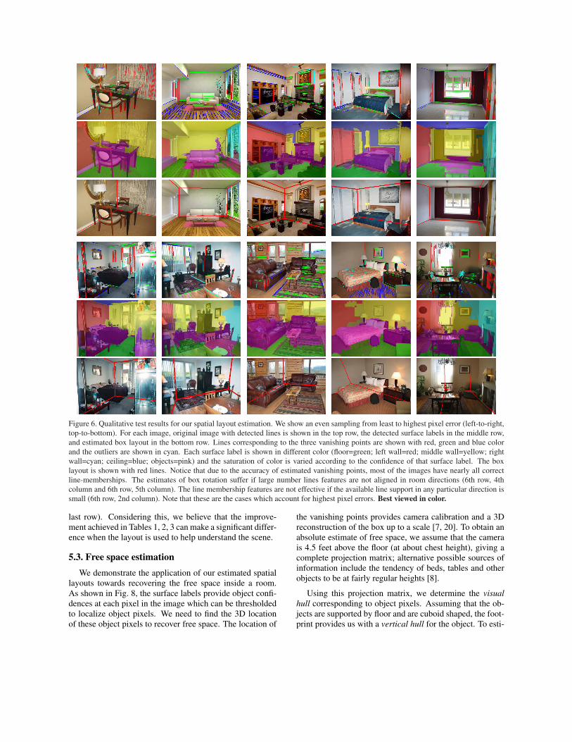
Figure 6. Qualitative test results for our spatial layout estimation. We show an even sampling from least to highest pixel error (left-to-right,top-to-bottom). For each image, original image with detected lines is shown in the top row, the detected surface labels in the middle row,and estimated box layout in the bottom row. Lines corresponding to the three vanishing points are shown with red, green and blue colorand the outliers are shown in cyan. Each surface label is shown in different color (floor=green; left wall=red; middle wall=yellow; rightwall=cyan; ceiling=blue; objects=pink) and the saturation of color is varied according to the confidence of that surface label. The boxlayout is shown with red lines. Notice that due to the accuracy of estimated vanishing points, most of the images have nearly all correctline-memberships. The estimates of box rotation suffer if large number lines features are not aligned in room directions (6th row, 4thcolumn and 6th row, 5th column). The line membership features are not effective if the available line support in any particular direction issmall (6th row, 2nd column). Note that these are the cases which account for highest pixel errors. Best viewed in color.
last row). Considering this, we believe that the improve-ment achieved in Tables 1, 2, 3 can make a significant differ-ence when the layout is used to help understand the scene.
5.3. Free space estimationWe demonstrate the application of our estimated spatial
layouts towards recovering the free space inside a room.As shown in Fig. 8, the surface labels provide object confi-dences at each pixel in the image which can be thresholdedto localize object pixels. We need to find the 3D locationof these object pixels to recover free space. The location of
the vanishing points provides camera calibration and a 3Dreconstruction of the box up to a scale [7, 20]. To obtain anabsolute estimate of free space, we assume that the camerais 4.5 feet above the floor (at about chest height), giving acomplete projection matrix; alternative possible sources ofinformation include the tendency of beds, tables and otherobjects to be at fairly regular heights [8].
Using this projection matrix, we determine the visualhull corresponding to object pixels. Assuming that the ob-jects are supported by floor and are cuboid shaped, the foot-print provides us with a vertical hull for the object. To esti-
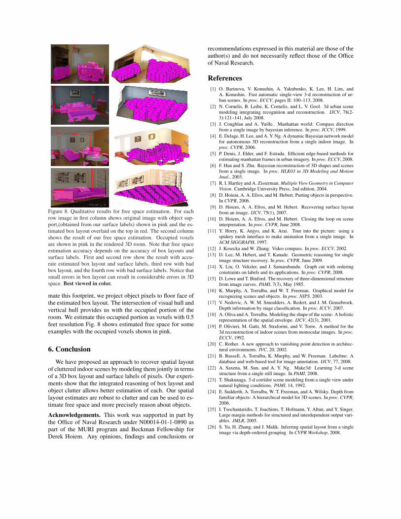
Figure 8. Qualitative results for free space estimation. For eachrow image in first column shows original image with object sup-port,(obtained from our surface labels) shown in pink and the es-timated box layout overlaid on the top in red. The second columnshows the result of our free space estimation. Occupied voxelsare shown in pink in the rendered 3D room. Note that free spaceestimation accuracy depends on the accuracy of box layouts andsurface labels. First and second row show the result with accu-rate estimated box layout and surface labels, third row with badbox layout, and the fourth row with bad surface labels. Notice thatsmall errors in box layout can result in considerable errors in 3Dspace. Best viewed in color.
mate this footprint, we project object pixels to floor face ofthe estimated box layout. The intersection of visual hull andvertical hull provides us with the occupied portion of theroom. We estimate this occupied portion as voxels with 0.5feet resolution Fig. 8 shows estimated free space for someexamples with the occupied voxels shown in pink.
6. Conclusion
We have proposed an approach to recover spatial layoutof cluttered indoor scenes by modeling them jointly in termsof a 3D box layout and surface labels of pixels. Our experi-ments show that the integrated reasoning of box layout andobject clutter allows better estimation of each. Our spatiallayout estimates are robust to clutter and can be used to es-timate free space and more precisely reason about objects.
Acknowledgements. This work was supported in part bythe Office of Naval Research under N00014-01-1-0890 aspart of the MURI program and Beckman Fellowship forDerek Hoiem. Any opinions, findings and conclusions or
recommendations expressed in this material are those of theauthor(s) and do not necessarily reflect those of the Officeof Naval Research.
References[1] O. Barinova, V. Konushin, A. Yakubenko, K. Lee, H. Lim, and
A. Konushin. Fast automatic single-view 3-d reconstruction of ur-ban scenes. In proc. ECCV, pages II: 100–113, 2008.
[2] N. Cornelis, B. Leibe, K. Cornelis, and L. V. Gool. 3d urban scenemodeling integrating recognition and reconstruction. IJCV, 78(2-3):121–141, July 2008.
[3] J. Coughlan and A. Yuille. Manhattan world: Compass directionfrom a single image by bayesian inference. In proc. ICCV, 1999.
[4] E. Delage, H. Lee, and A. Y. Ng. A dynamic Bayesian network modelfor autonomous 3D reconstruction from a single indoor image. Inproc. CVPR, 2006.
[5] P. Denis, J. Elder, and F. Estrada. Efficient edge-based methods forestimating manhattan frames in urban imagery. In proc. ECCV, 2008.
[6] F. Han and S. Zhu. Bayesian reconstruction of 3D shapes and scenesfrom a single image. In proc. HLK03 in 3D Modeling and MotionAnal., 2003.
[7] R. I. Hartley and A. Zisserman. Multiple View Geometry in ComputerVision. Cambridge University Press, 2nd edition, 2004.
[8] D. Hoiem, A. A. Efros, and M. Hebert. Putting objects in perspective.In CVPR, 2006.
[9] D. Hoiem, A. A. Efros, and M. Hebert. Recovering surface layoutfrom an image. IJCV, 75(1), 2007.
[10] D. Hoiem, A. A. Efros, and M. Hebert. Closing the loop on sceneinterpretation. In proc. CVPR, June 2008.
[11] Y. Horry, K. Anjyo, and K. Arai. Tour into the picture: using aspidery mesh interface to make animation from a single image. InACM SIGGRAPH, 1997.
[12] J. Kosecka and W. Zhang. Video compass. In proc. ECCV, 2002.[13] D. Lee, M. Hebert, and T. Kanade. Geometric reasoning for single
image structure recovery. In proc. CVPR, June 2009.[14] X. Liu, O. Veksler, and J. Samarabandu. Graph cut with ordering
constraints on labels and its applications. In proc. CVPR, 2008.[15] D. Lowe and T. Binford. The recovery of three-dimensional structure
from image curves. PAMI, 7(3), May 1985.[16] K. Murphy, A. Torralba, and W. T. Freeman. Graphical model for
recognizing scenes and objects. In proc. NIPS. 2003.[17] V. Nedovic, A. W. M. Smeulders, A. Redert, and J. M. Geusebroek.
Depth information by stage classification. In proc. ICCV, 2007.[18] A. Oliva and A. Torralba. Modeling the shape of the scene: A holistic
representation of the spatial envelope. IJCV, 42(3), 2001.[19] P. Olivieri, M. Gatti, M. Straforini, and V. Torre. A method for the
3d reconstruction of indoor scenes from monocular images. In proc.ECCV, 1992.
[20] C. Rother. A new approach to vanishing point detection in architec-tural environments. IVC, 20, 2002.
[21] B. Russell, A. Torralba, K. Murphy, and W. Freeman. Labelme: Adatabase and web-based tool for image annotation. IJCV, 77, 2008.
[22] A. Saxena, M. Sun, and A. Y. Ng. Make3d: Learning 3-d scenestructure from a single still image. In PAMI, 2008.
[23] T. Shakunaga. 3-d corridor scene modeling from a single view undernatural lighting conditions. PAMI, 14, 1992.
[24] E. Sudderth, A. Torralba, W. T. Freeman, and A. Wilsky. Depth fromfamiliar objects: A hierarchical model for 3D scenes. In proc. CVPR,2006.
[25] I. Tsochantaridis, T. Joachims, T. Hofmann, Y. Altun, and Y. Singer.Large margin methods for structured and interdependent output vari-ables. JMLR, 2005.
[26] S. Yu, H. Zhang, and J. Malik. Inferring spatial layout from a singleimage via depth-ordered grouping. In CVPR Workshop, 2008.