Recent Developments in Proton-Detected

Solid-State NMR A literature study

Breuer, Pascal 8/16/17 Literature Thesis

MSc Chemistry

Track Analytical Sciences

Literature Thesis

Recent Developments in

Proton-Detected Solid-State

NMR

by

Pascal Breuer

10881522

August 2017

12EC

June 2017 – August 2017

Supervisor/Examiner: Examiner:

E.A.W. van der Cruijsen, Dr. W.Th Kok, Dr.

DSM Coating Resins

Recent Developments in

Proton-Detected Solid-State

NMR A literature study

Approval Name: Breuer, Pascal APPROVED BY: E.A.W. van der Cruijsen, Dr. Daily Supervisor DSM Scientist – Compliance __________________________________________________ Date: R. Peters, Prof. Dr. Manager DSM Science Manager Analytics __________________________________________________ Date: W.Th. Kok, Dr. First Examinator __________________________________________________ Date: Second Examinator __________________________________________________ Date:

Abstract A vast majority of the NMR analysis are performed in the solution-state. However, certain samples, especially in the polymer industry, suffer from limited solubility, thus require analysis by solid-state NMR. This technique was limited to only use less sensitive spins like 13C and 15N, due to servere line-broadening caused by dipolar couplings and chemical shift anisotropy. While these type of interactions are averaged out by fast tumbling of the molecules in solution-state NMR, they are well expressed in solid-state NMR. The wide chemical shift window of 13C and 15N made those nuclei favorable to measure in comparison to the narrow chemical shift window of protons. While the broad spectra do contain a lot of information, it cannot be extracted due to too limited resolution. Recent developments in ultra-fast magic angle spinning probes in combination with advanced radio frequency pulse schemes, allow for averaging out chemical shift anisotropies and selectively decouple and recouple dipolar interactions. As a result, high-resolution proton spectra can be recorded, which provides a large increase in information either by performing one- or multidimensional solid-state NMR analysis. In this literature research, the basic theoretical knowledge with respect to the line-broadening is addressed, followed by current solutions such as magic-angle spinning and radio-frequency pulse schemes. Last, applications are presented, which show the current possibilities of proton-detected solid-state NMR. This includes ultra-fast magic angle spinning probes in high magnetic field (>1 GHz), structure determination of proteins and both hydrogen bonding and dynamics in polymers.

IV

Table of Contents Approval ......................................................................................................................................... IV

Abstract ........................................................................................................................................... V

1. Introduction .............................................................................................................................. 1

2. Theory ....................................................................................................................................... 4

2.1. Basic principles .................................................................................................................. 4

2.1.1. Chemical shift ............................................................................................................. 4

2.1.2. Spin-spin coupling ...................................................................................................... 5

2.2. Magic angle spinning ......................................................................................................... 7

2.3. Decoupling schemes .......................................................................................................... 8

2.3.1. PMLG .......................................................................................................................... 9

2.3.2. DUMBO ..................................................................................................................... 12

2.4. Cross-polarization ............................................................................................................ 14

2.5. Multidimensional NMR .................................................................................................... 15

3. Applications ............................................................................................................................. 17

3.1. Morphology by 13C solid-state NMR ................................................................................ 17

3.2. High-resolution proton solid-state NMR ......................................................................... 17

3.3. Protein structure determination ..................................................................................... 22

3.4. Hydrogen bond interaction and dynamics in polymer blends ........................................ 26

4. Conclusion/summary .............................................................................................................. 30

5. Literature................................................................................................................................. 32

List of Abbreviations and Notations ............................................................................................... 37

[1]

1. Introduction It was already in the early 1920’s that the concept of electron spin and magnetic moment of the electron was widely established. However, it was in 1946 that the first two NMR measurements were reported by Bloch, Hansen and Packard at Stanford [1], and Purcell, Torrey and Pound at Harvard [2]. Already in 1952 both Bloch and Purcell received the Nobel Prize in Physics for their discovery. Surprisingly Bloch and Purcell did not know each other back in 1946, while their paper on the topic of NMR was published just weeks apart. In 1948, Bloembergen, Purcell and Pound came up with the concept of nuclear relaxation [3], which addressed why the width of NMR signals of solids are far larger than liquids, which even today is still a challenge to overcome. They explained that, in liquids, rapid molecular Brownian motion averages the dipole-dipole interaction to zero. However, in solids molecules are fixed in a certain position and therefore don’t show the rapid molecular Brownian motion. Thus, instead of an average NMR signal from all the fast tumbling molecules, solids show a wide array of NMR signals corresponding to all the molecules oriented at different positions. While the magnets became better in time, the observed resonance lines in liquids became sharper. The anticipation rose that the same frequency would be observed for a certain nucleus at a specific applied magnetic field, regardless of its surrounding. The first relationship was born: 𝝎 = 𝜸𝑩𝒏𝒖𝒄𝒍𝒆𝒖𝒔 ( 1 )

ω is the resonance frequency which is given by the magnetogyric ratio (γ) of the nucleus multiplied by the applied magnetic field (Bnucleus) to the nucleus. In the following years, new results showed that Formula 1 does not hold up, due to large variations observed especially from 19F and 31P. This lead to the concept of chemical shielding, which explains the effect of surrounding electrons on the effective magnetic field which is felt by the nucleus. Formula 1 was adjusted to account for chemical shielding: 𝝎 = 𝜸𝑩𝟎(𝟏 − 𝝈) ( 2 )

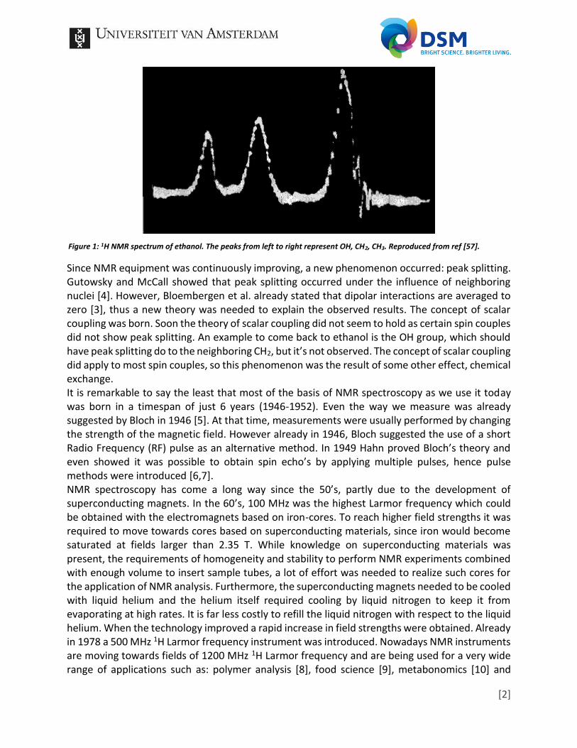
B0 is the applied magnetic field and σ is the chemical shielding which depends not only on the density of the electrons around the nucleus, but also their configuration. The difference between Formula 1 and 2 is the parameter which became one of the most important parameters in chemistry when applying NMR spectroscopy: the chemical shift. While one might not realize it, the chemical shift of 1H, which is the most often measured nucleus nowadays, could only be proved after the homogeneity and stability of the applied magnetic fields were improved. The chemical shift of 1H is in the range of roughly 0 - 15 ppm, a chemical shift window which was too limited compared to the relatively broad lines observed. Thus, line narrowing was needed to observe the 1H chemical shifts. As a result, the most common NMR experiments at that time were 19F and 31P which have a chemical shift range above 100 ppm. Another advantage is the 100% abundance for both nuclei. While 13C also shows a large chemical shift range, its natural abundance is just above 1%. The lack of sensitivity made 13C experiments unfavorable. When line-narrowing was achieved the first 1H-spectra were measured. A very famous example is the NMR spectrum of ethanol as is shown in Figure 1. This spectrum from 1951 proved that NMR could be used as an analytical method for chemists, instead of being solely useful to physicists.

[2]

Since NMR equipment was continuously improving, a new phenomenon occurred: peak splitting. Gutowsky and McCall showed that peak splitting occurred under the influence of neighboring nuclei [4]. However, Bloembergen et al. already stated that dipolar interactions are averaged to zero [3], thus a new theory was needed to explain the observed results. The concept of scalar coupling was born. Soon the theory of scalar coupling did not seem to hold as certain spin couples did not show peak splitting. An example to come back to ethanol is the OH group, which should have peak splitting do to the neighboring CH2, but it’s not observed. The concept of scalar coupling did apply to most spin couples, so this phenomenon was the result of some other effect, chemical exchange. It is remarkable to say the least that most of the basis of NMR spectroscopy as we use it today was born in a timespan of just 6 years (1946-1952). Even the way we measure was already suggested by Bloch in 1946 [5]. At that time, measurements were usually performed by changing the strength of the magnetic field. However already in 1946, Bloch suggested the use of a short Radio Frequency (RF) pulse as an alternative method. In 1949 Hahn proved Bloch’s theory and even showed it was possible to obtain spin echo’s by applying multiple pulses, hence pulse methods were introduced [6,7]. NMR spectroscopy has come a long way since the 50’s, partly due to the development of superconducting magnets. In the 60’s, 100 MHz was the highest Larmor frequency which could be obtained with the electromagnets based on iron-cores. To reach higher field strengths it was required to move towards cores based on superconducting materials, since iron would become saturated at fields larger than 2.35 T. While knowledge on superconducting materials was present, the requirements of homogeneity and stability to perform NMR experiments combined with enough volume to insert sample tubes, a lot of effort was needed to realize such cores for the application of NMR analysis. Furthermore, the superconducting magnets needed to be cooled with liquid helium and the helium itself required cooling by liquid nitrogen to keep it from evaporating at high rates. It is far less costly to refill the liquid nitrogen with respect to the liquid helium. When the technology improved a rapid increase in field strengths were obtained. Already in 1978 a 500 MHz 1H Larmor frequency instrument was introduced. Nowadays NMR instruments are moving towards fields of 1200 MHz 1H Larmor frequency and are being used for a very wide range of applications such as: polymer analysis [8], food science [9], metabonomics [10] and

Figure 1: 1H NMR spectrum of ethanol. The peaks from left to right represent OH, CH2, CH3. Reproduced from ref [57].

[3]

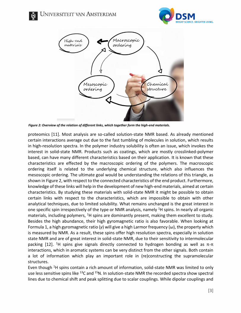
proteomics [11]. Most analysis are so-called solution-state NMR based. As already mentioned certain interactions average out due to the fast tumbling of molecules in solution, which results in high-resolution spectra. In the polymer industry solubility is often an issue, which invokes the interest in solid-state NMR. Products such as coatings, which are mostly crosslinked-polymer based, can have many different characteristics based on their application. It is known that these characteristics are effected by the macroscopic ordering of the polymers. The macroscopic ordering itself is related to the underlying chemical structure, which also influences the mesoscopic ordering. The ultimate goal would be understanding the relations of this triangle, as shown in Figure 2, with respect to the connected characteristics of the end product. Furthermore, knowledge of these links will help in the development of new high-end materials, aimed at certain characteristics. By studying these materials with solid-state NMR it might be possible to obtain certain links with respect to the characteristics, which are impossible to obtain with other analytical techniques, due to limited solubility. What remains unchanged is the great interest in one specific spin irrespectively of the type or NMR analysis, namely 1H spins. In nearly all organic materials, including polymers, 1H spins are dominantly present, making them excellent to study. Besides the high abundance, their high gyromagnetic ratio is also favorable. When looking at Formula 1, a high gyromagnetic ratio (γ) will give a high Larmor frequency (ω), the property which is measured by NMR. As a result, these spins offer high resolution spectra, especially in solution state NMR and are of great interest in solid-state NMR, due to their sensitivity to intermolecular packing [12]. 1H spins give signals directly connected to hydrogen bonding as well as π-π interactions, which in aromatic systems can be very distinct from the other signals. Both contain a lot of information which play an important role in (re)constructing the supramolecular structures. Even though 1H spins contain a rich amount of information, solid-state NMR was limited to only use less sensitive spins like 13C and 15N. In solution-state NMR the recorded spectra show spectral lines due to chemical shift and peak splitting due to scalar couplings. While dipolar couplings and

Figure 2: Overview of the relation of different links, which together form the high-end materials.

[4]

chemical shift anisotropy may contribute to the lines, they are averaged out due to fast random tumbling of the molecules in solution. In solid-state this is not the case. All the different orientations which are present in the solid sample give rise to a signal belonging to that specific orientation. Thus, instead of a sharp peak corresponding to the average, a very broad spectrum is obtained in which the dipolar couplings and chemical shift anisotropy are present. However, broader line widths also mean a reduced resolution. While the spectra are by definition rich in information, the resolution is not sufficient to extract it. A logical solution is mimicking the fast, random tumbling by moving the solid sample by artificial means. This technique is better known as Magic Angle Spinning (MAS). The specifics of MAS will be addressed in the Theory. While MAS does improve the obtained signals significantly, it is often not enough. While inhomogeneous signals are averaged out, the strong 1H-1H homonuclear dipolar interactions prove to be difficult. These specific interactions can reach up to 100 kHz, thus the magic angle spinning rate needs to be even higher to average out the interactions. While ultra-fast MAS is currently commercially available, there are other methods to obtain high resolution spectra. By applying RF pulse methods it is possible to decouple certain interactions, sharpening the spectra. In this research, the first work in homonuclear dipolar decoupling will be discussed, including currently popular decoupling schemes. While both MAS and decoupling can be used separately, combining them improves the obtained results. This is better known as Combined Rotation And Multiple-Pulse Spectroscopy (CRAMPS). Some other methods which should be known by every solid-state NMR annalist are dilution and Cross-Polarization (CP). While the previous mentioned methods are specifically developed for solid-state NMR, dilution is used in solution-state NMR as well.

2. Theory In this chapter, multiple subjects will be addressed. First some basic principles will be explained to create a basis, which the more advanced theory relies on. Second, magic angle spinning will be explained, which is commonly used in solid-state NMR. Next, two different methods will be explained, decoupling and cross polarization, which could be performed in combination with magic angle spinning to increase the obtained resolution. Last, multidimensional NMR will be addressed, due to the increase of information gain in such an experiment.

2.1. Basic principles

In this paragraph the chemical shift, on which the interpretation of the spectra relies, will be further explained. Next, spin-spin couplings will be explained, which are the main reason that solid-state NMR requires certain methods to obtain high-resolution spectra.

2.1.1. Chemical shift

In the introduction, Formula 2 describes the concept of chemical shift. A nucleus “feels” an applied external field and spins therefore move accordingly with a certain Lamor frequency. However, the measured Lamor frequency differs from the predicted frequency due to chemical shielding. When a nucleus is exposed to an external magnetic field, a local induced magnetic field will be present on a nuclear site. The combination of this local magnetic field and the applied magnetic field results in the effective magnetic field. The effective field is dependent on the electron density, thus dependent on the orientation of the molecule. This is better known as

[5]

Chemical Shift Anisotropy (CSA). To describe the effect of the electron density the shielding tensor σ is introduced with the following relation: 𝑩𝒆𝒇𝒇 = −𝝈𝑩𝟎 + 𝑩𝟎 ( 3 )

The term -σB0 represents the induced field Bind. The shielding tensor is a so-called second-rank tensor and can be described with a 3 x 3 matrix, corresponding to the three dimensional representation:

𝑩𝒊𝒏𝒅 = [

𝝈𝒙𝒙 𝝈𝒙𝒚 𝝈𝒙𝒛

𝝈𝒚𝒙 𝝈𝒚𝒚 𝝈𝒚𝒛

𝝈𝒛𝒙 𝝈𝒛𝒚 𝝈𝒛𝒛

] [𝟎𝟎

𝑩𝟎

] ( 4 )

A more common way to represent the shielding tensor is by plotting the principal components (the diagonal of the σ-matrix) on a principal axis system (an x, y, z axis). σzz Usually represents the largest vector. In solution-state NMR anisotropic effects are (mostly) averaged out by rapid tumbling, thus a nucleus shows a single narrow line in the chemical shift spectrum. This line corresponds to the isotropic chemical shift (δiso). From the above mentioned follows that the isotropic chemical shielding (σiso) is the average of the diagonal as they all contribute in the same ratio due to the rapid tumbling:

𝝈𝒊𝒔𝒐 =𝟏

𝟑 (𝝈𝒙𝒙 + 𝝈𝒚𝒚 + 𝝈𝒛𝒛) ( 5 )

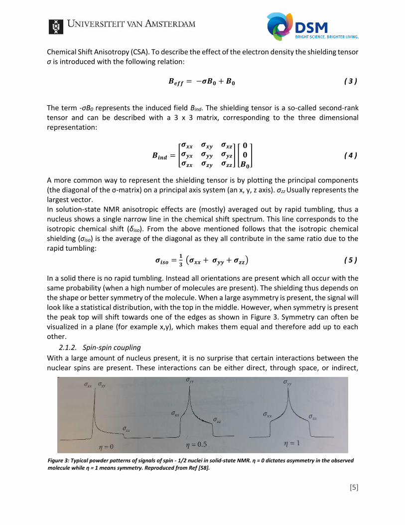
In a solid there is no rapid tumbling. Instead all orientations are present which all occur with the same probability (when a high number of molecules are present). The shielding thus depends on the shape or better symmetry of the molecule. When a large asymmetry is present, the signal will look like a statistical distribution, with the top in the middle. However, when symmetry is present the peak top will shift towards one of the edges as shown in Figure 3. Symmetry can often be visualized in a plane (for example x,y), which makes them equal and therefore add up to each other.

2.1.2. Spin-spin coupling

With a large amount of nucleus present, it is no surprise that certain interactions between the nuclear spins are present. These interactions can be either direct, through space, or indirect,

Figure 3: Typical powder patterns of signals of spin - 1/2 nuclei in solid-state NMR. η = 0 dictates asymmetry in the observed molecule while η = 1 means symmetry. Reproduced from Ref [58].

[6]

through electrons. Direct interactions are captured within the term dipolar couplings. Indirect interactions are called scalar couplings. The latter depends on neighboring electrons and causes resonance lines to split. Usually, the interaction only applies between those electrons which are no more than three bond lengths apart. As the name scalar coupling suggests, the spin-spin coupling depends on the scalar product between two spins. The energy of the interaction is denoted by the scalar tensor J. Just as the chemical shielding, the scalar coupling is averaged in solution-state NMR, resulting in a single value known as the scalar coupling constant. Again, the situation is different in solid-state NMR, where averaging does not occur. However, J-couplings are hard to observe due to the large line-widths in solid-state NMR. Still, if observable they are of great interest. J-couplings provide insight in the distances and orientation between certain nuclei, which helps in understanding the observed material on the sub nanometer scale. Direct spin-spin couplings are caused by the magnetic moments of the nuclear spins itself. It can best be compared with two small magnets in close proximity, they will feel each other. The interaction between these local fields is the dipolar coupling. The relation is given by:

𝒅𝑰 𝑺 = 𝝁𝟎𝜸𝑰𝜸𝑺

ħ

𝟒𝝅∗

𝟏

𝒓𝑰 𝑺𝟑 ( 6 )

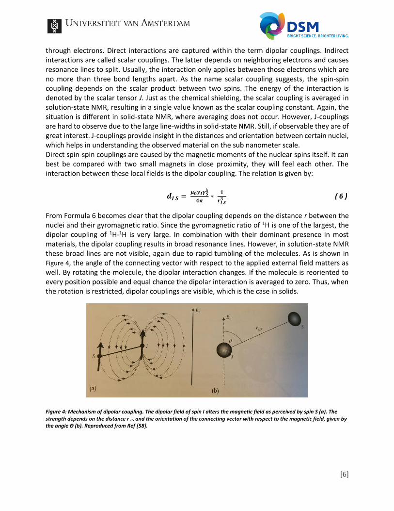
From Formula 6 becomes clear that the dipolar coupling depends on the distance r between the nuclei and their gyromagnetic ratio. Since the gyromagnetic ratio of 1H is one of the largest, the dipolar coupling of 1H-1H is very large. In combination with their dominant presence in most materials, the dipolar coupling results in broad resonance lines. However, in solution-state NMR these broad lines are not visible, again due to rapid tumbling of the molecules. As is shown in Figure 4, the angle of the connecting vector with respect to the applied external field matters as well. By rotating the molecule, the dipolar interaction changes. If the molecule is reoriented to every position possible and equal chance the dipolar interaction is averaged to zero. Thus, when the rotation is restricted, dipolar couplings are visible, which is the case in solids.

Figure 4: Mechanism of dipolar coupling. The dipolar field of spin I alters the magnetic field as perceived by spin S (a). The strength depends on the distance r I S and the orientation of the connecting vector with respect to the magnetic field, given by the angle ϴ (b). Reproduced from Ref [58].

[7]

2.2. Magic angle spinning

As explained both CSA and dipolar coupling are present in solids, which results in very broad resonance lines. While in theory a lot of information should be present in the spectrum, resolution is to limited to deduct the information. Since rapid tumbling averages out both CSA and dipolar coupling, the same should be possible in solid-state NMR by mimicking the rapid tumbling. Simply rotating the sample at high speeds is not sufficient, it needs to be done at a specific angle, the so-called magic angle. Most interactions can be described by a Hamiltonian, including the dipolar coupling:

𝑯𝒅 = 𝒅−𝟑 ∗ (𝟑𝒄𝒐𝒔𝟐 𝜽 − 𝟏) ∗ 𝑰𝒛𝑺𝒛 ( 7 )

MAS focusses on bringing the term within the brackets to approach zero. Rotation is achieved by a small rotor, usually between the 0.8 and 7 mm in outer diameter. By applying a certain air pressure the rotor will rotate at a specific frequency. This frequency is limited by multiple factors such as mechanical eigen frequency, frictional loss at the rotor surface, and the strength of the applied materials to withstand the centrifugal forces among multiple others [13]. In practice it means that the maximum spinning speed should be in the order of three quarters of the speed of sound:

𝒗𝒎𝒂𝒙 = 𝟎. 𝟕𝟓 𝒄

𝝅𝒅 ( 8 )

From Formula 8 can be conducted that the maximum rotor frequency depends on the speed of sound and the rotor diameter. When working at ambient temperature and with compressed air, Formula 8 can be rewritten to show the relation between vmax and the rotor diameter:

𝒗𝒎𝒂𝒙 =𝟖𝟎 𝒌𝑯𝒛 𝒎𝒎−𝟏

𝒅 ( 9 )

As mentioned, the dipolar coupling between 1H spins can be as large as 100 kHz. According to Formula 9 a rotor diameter of 0.8 mm or less is required to reach a spinning frequency of 100 kHz or higher. While in principle the speed of sound can be changed as well by applying for example helium gas, the issue of heating rises. Both Formula 8 and 9 explain the move towards smaller and smaller rotors. However, not without sacrificing sample volume. While increasing the length of the rotor might seem an option, the mechanical eigen frequency limits the length to a large extent. When the oscillations of the rotor start to match with its eigen frequency (vibration), the rotating system can become extremely unstable or even “spin out of control”. A nice example of resonance is the “dancing” Tacoma Narrows Bridge back in 1940. It should not require any further explanation that one should avoid a crashing rotor which is spinning a very high frequencies. The maximum length/diameter ratio to obtain the optimal sample volume without lowering the maximum spinning frequency is given by [14]

(𝒍

𝒅) < (

𝟏

𝟖𝒄)

𝟏

𝟐((𝟏 + (

𝒅𝒊𝒏

𝒅)

𝟐

)𝑬

𝝆) 𝑩𝟏/𝟐 ( 10 )

[8]

While the formula is somewhat complex, it summarizes to a l/d ratio of 5-7 irrespectively of the rotor diameter. Assuming constant ratios in Formula 10 and the optimal l/d ratio an estimate of the sample volume can be given by 𝒗𝒔𝒂𝒎𝒑𝒍𝒆 = 𝒂𝒅𝟑 ( 11 )

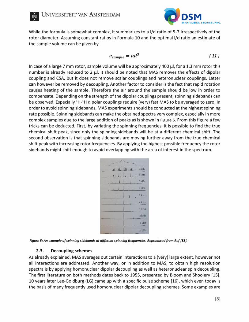
In case of a large 7 mm rotor, sample volume will be approximately 400 µl, for a 1.3 mm rotor this number is already reduced to 2 µl. It should be noted that MAS removes the effects of dipolar coupling and CSA, but it does not remove scalar couplings and heteronuclear couplings. Latter can however be removed by decoupling. Another factor to consider is the fact that rapid rotation causes heating of the sample. Therefore the air around the sample should be low in order to compensate. Depending on the strength of the dipolar couplings present, spinning sidebands can be observed. Especially 1H-1H dipolar couplings require (very) fast MAS to be averaged to zero. In order to avoid spinning sidebands, MAS experiments should be conducted at the highest spinning rate possible. Spinning sidebands can make the obtained spectra very complex, especially in more complex samples due to the large addition of peaks as is shown in Figure 5. From this figure a few tricks can be deducted. First, by variating the spinning frequencies, it is possible to find the true chemical shift peak, since only the spinning sidebands will be at a different chemical shift. The second observation is that spinning sidebands are moving further away from the true chemical shift peak with increasing rotor frequencies. By applying the highest possible frequency the rotor sidebands might shift enough to avoid overlapping with the area of interest in the spectrum.

2.3. Decoupling schemes

As already explained, MAS averages out certain interactions to a (very) large extent, however not all interactions are addressed. Another way, or in addition to MAS, to obtain high resolution spectra is by applying homonuclear dipolar decoupling as well as heteronuclear spin decoupling. The first literature on both methods dates back to 1955, presented by Bloom and Shoolery [15]. 10 years later Lee-Goldburg (LG) came up with a specific pulse scheme [16], which even today is the basis of many frequently used homonuclear dipolar decoupling schemes. Some examples are

Figure 5: An example of spinning sidebands at different spinning frequencies. Reproduced from Ref [58].

[9]

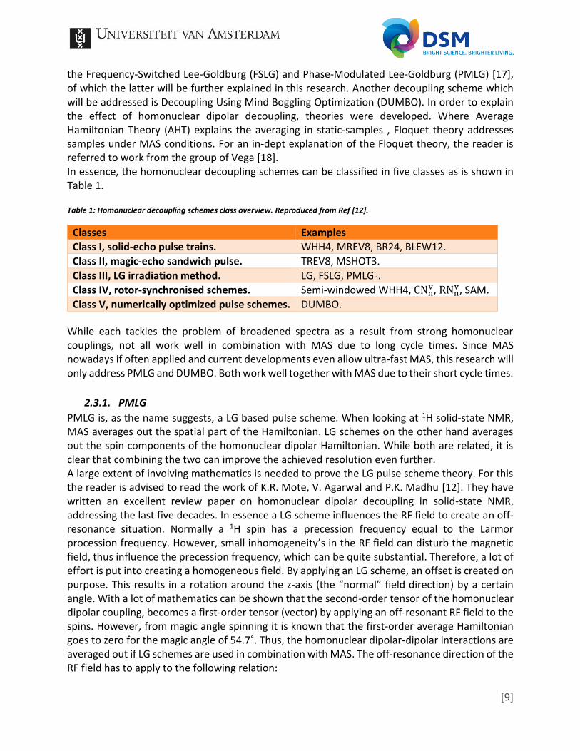
the Frequency-Switched Lee-Goldburg (FSLG) and Phase-Modulated Lee-Goldburg (PMLG) [17], of which the latter will be further explained in this research. Another decoupling scheme which will be addressed is Decoupling Using Mind Boggling Optimization (DUMBO). In order to explain the effect of homonuclear dipolar decoupling, theories were developed. Where Average Hamiltonian Theory (AHT) explains the averaging in static-samples , Floquet theory addresses samples under MAS conditions. For an in-dept explanation of the Floquet theory, the reader is referred to work from the group of Vega [18]. In essence, the homonuclear decoupling schemes can be classified in five classes as is shown in Table 1. Table 1: Homonuclear decoupling schemes class overview. Reproduced from Ref [12].

Classes Examples

Class I, solid-echo pulse trains. WHH4, MREV8, BR24, BLEW12.

Class II, magic-echo sandwich pulse. TREV8, MSHOT3.

Class III, LG irradiation method. LG, FSLG, PMLGn.

Class IV, rotor-synchronised schemes. Semi-windowed WHH4, CNnv, RNn

v, SAM.

Class V, numerically optimized pulse schemes. DUMBO.

While each tackles the problem of broadened spectra as a result from strong homonuclear couplings, not all work well in combination with MAS due to long cycle times. Since MAS nowadays if often applied and current developments even allow ultra-fast MAS, this research will only address PMLG and DUMBO. Both work well together with MAS due to their short cycle times.

2.3.1. PMLG

PMLG is, as the name suggests, a LG based pulse scheme. When looking at 1H solid-state NMR, MAS averages out the spatial part of the Hamiltonian. LG schemes on the other hand averages out the spin components of the homonuclear dipolar Hamiltonian. While both are related, it is clear that combining the two can improve the achieved resolution even further. A large extent of involving mathematics is needed to prove the LG pulse scheme theory. For this the reader is advised to read the work of K.R. Mote, V. Agarwal and P.K. Madhu [12]. They have written an excellent review paper on homonuclear dipolar decoupling in solid-state NMR, addressing the last five decades. In essence a LG scheme influences the RF field to create an off-resonance situation. Normally a 1H spin has a precession frequency equal to the Larmor procession frequency. However, small inhomogeneity’s in the RF field can disturb the magnetic field, thus influence the precession frequency, which can be quite substantial. Therefore, a lot of effort is put into creating a homogeneous field. By applying an LG scheme, an offset is created on purpose. This results in a rotation around the z-axis (the “normal” field direction) by a certain angle. With a lot of mathematics can be shown that the second-order tensor of the homonuclear dipolar coupling, becomes a first-order tensor (vector) by applying an off-resonant RF field to the spins. However, from magic angle spinning it is known that the first-order average Hamiltonian goes to zero for the magic angle of 54.7˚. Thus, the homonuclear dipolar-dipolar interactions are averaged out if LG schemes are used in combination with MAS. The off-resonance direction of the RF field has to apply to the following relation:

[10]

𝜽 = 𝒕𝒂𝒏−𝟏 𝒗𝟏

∆𝒗= 𝒕𝒂𝒏−𝟏 √𝟐 ( 12 )

Thus, 𝜟𝒗 =𝒗𝟏

√𝟐 , else the dipolar interactions will not become first order tensors.

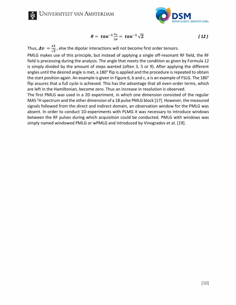
PMLG makes use of this principle, but instead of applying a single off-resonant RF field, the RF field is precessing during the analysis. The angle that meets the condition as given by Formula 12 is simply divided by the amount of steps wanted (often 3, 5 or 9). After applying the different angles until the desired angle is met, a 180° flip is applied and the procedure is repeated to obtain the start position again. An example is given in Figure 6, b and c, a is an example of FSLG. The 180° flip assures that a full cycle is achieved. This has the advantage that all even-order terms, which are left in the Hamiltonian, become zero. Thus an increase in resolution is observed. The first PMLG was used in a 2D experiment, in which one dimension consisted of the regular MAS 1H spectrum and the other dimension of a 18 pulse PMLG block [17]. However, the measured signals followed from the direct and indirect domain, an observation window for the PMLG was absent. In order to conduct 1D-experiments with PLMG it was necessary to introduce windows between the RF pulses during which acquisition could be conducted. PMLG with windows was simply named windowed PMLG or wPMLG and introduced by Vinogradov et al. [19].

[11]

Figure 6: Schematic of (a) FSLG, (b) PMLG9, and (c) wPMLG5. The left column shows the pulse blocks and their corresponding RF irradiation profiles in the xy plane of the rotating frame are given in the right column. Reproduced from Ref [12].

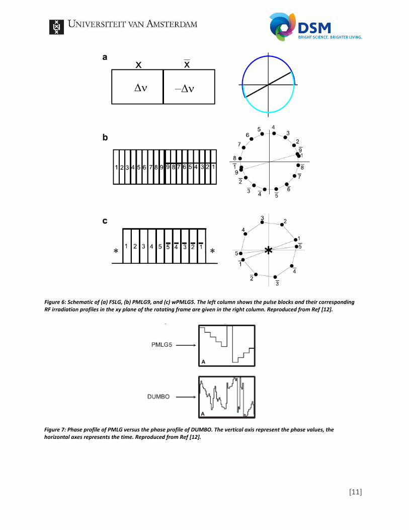
Figure 7: Phase profile of PMLG versus the phase profile of DUMBO. The vertical axis represent the phase values, the horizontal axes represents the time. Reproduced from Ref [12].

[12]

2.3.2. DUMBO

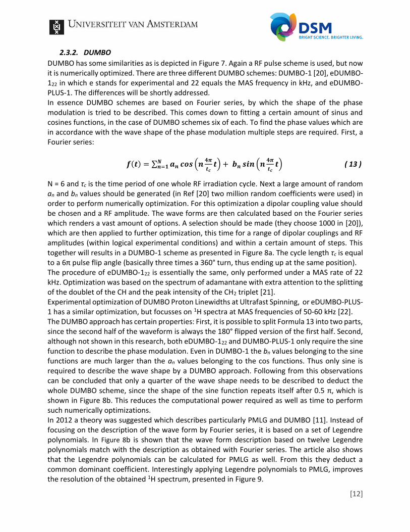
DUMBO has some similarities as is depicted in Figure 7. Again a RF pulse scheme is used, but now it is numerically optimized. There are three different DUMBO schemes: DUMBO-1 [20], eDUMBO-122 in which e stands for experimental and 22 equals the MAS frequency in kHz, and eDUMBO-PLUS-1. The differences will be shortly addressed. In essence DUMBO schemes are based on Fourier series, by which the shape of the phase modulation is tried to be described. This comes down to fitting a certain amount of sinus and cosines functions, in the case of DUMBO schemes six of each. To find the phase values which are in accordance with the wave shape of the phase modulation multiple steps are required. First, a Fourier series:

𝒇(𝒕) = ∑ 𝒂𝒏 𝒄𝒐𝒔 (𝒏𝟒𝝅

𝒕𝒄𝒕) + 𝒃𝒏 𝒔𝒊𝒏 (𝒏

𝟒𝝅

𝒕𝒄𝒕)𝑵

𝒏=𝟏 ( 13 )

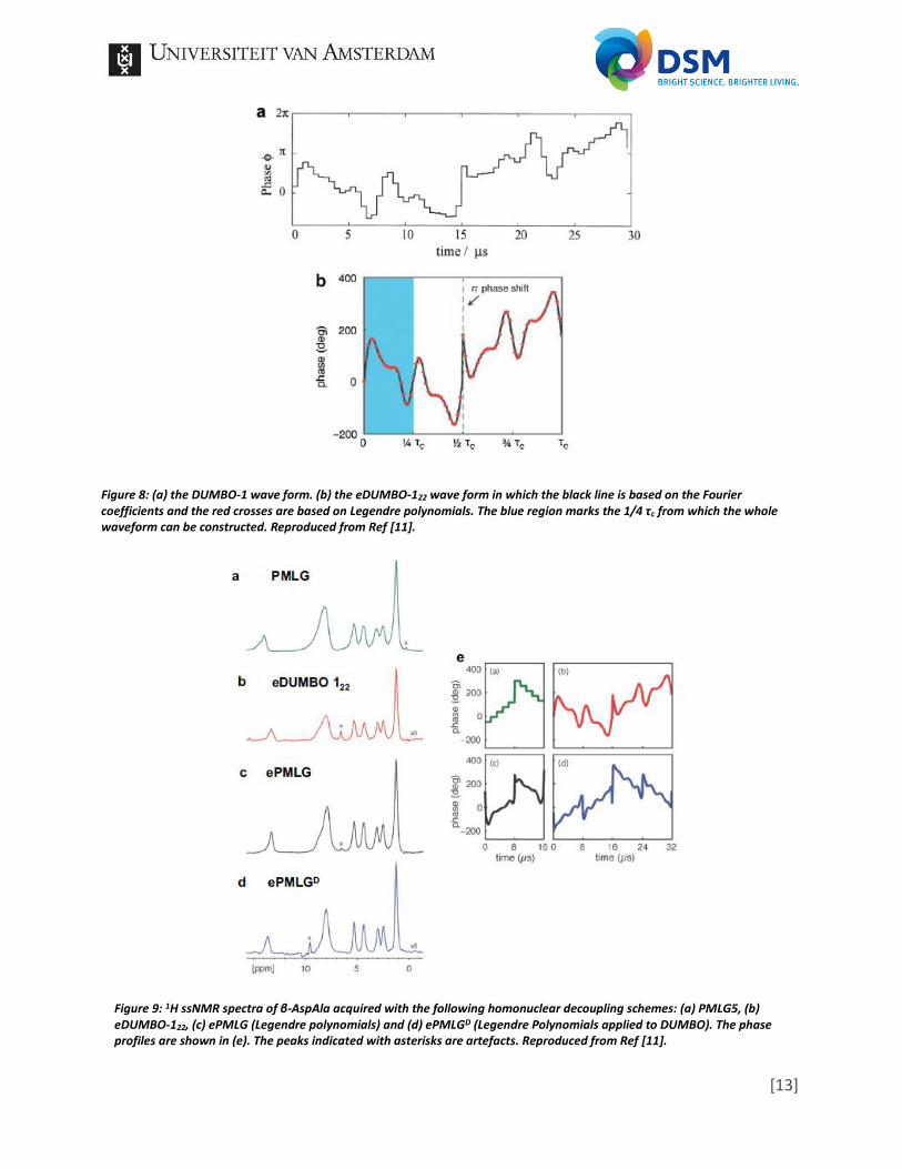
N = 6 and τc is the time period of one whole RF irradiation cycle. Next a large amount of random an and bn values should be generated (in Ref [20] two million random coefficients were used) in order to perform numerically optimization. For this optimization a dipolar coupling value should be chosen and a RF amplitude. The wave forms are then calculated based on the Fourier series which renders a vast amount of options. A selection should be made (they choose 1000 in [20]), which are then applied to further optimization, this time for a range of dipolar couplings and RF amplitudes (within logical experimental conditions) and within a certain amount of steps. This together will results in a DUMBO-1 scheme as presented in Figure 8a. The cycle length τc is equal to a 6π pulse flip angle (basically three times a 360° turn, thus ending up at the same position). The procedure of eDUMBO-122 is essentially the same, only performed under a MAS rate of 22 kHz. Optimization was based on the spectrum of adamantane with extra attention to the splitting of the doublet of the CH and the peak intensity of the CH2 triplet [21]. Experimental optimization of DUMBO Proton Linewidths at Ultrafast Spinning, or eDUMBO-PLUS-1 has a similar optimization, but focusses on 1H spectra at MAS frequencies of 50-60 kHz [22]. The DUMBO approach has certain properties: First, it is possible to split Formula 13 into two parts, since the second half of the waveform is always the 180° flipped version of the first half. Second, although not shown in this research, both eDUMBO-122 and DUMBO-PLUS-1 only require the sine function to describe the phase modulation. Even in DUMBO-1 the bn values belonging to the sine functions are much larger than the an values belonging to the cos functions. Thus only sine is required to describe the wave shape by a DUMBO approach. Following from this observations can be concluded that only a quarter of the wave shape needs to be described to deduct the whole DUMBO scheme, since the shape of the sine function repeats itself after 0.5 π, which is shown in Figure 8b. This reduces the computational power required as well as time to perform such numerically optimizations. In 2012 a theory was suggested which describes particularly PMLG and DUMBO [11]. Instead of focusing on the description of the wave form by Fourier series, it is based on a set of Legendre polynomials. In Figure 8b is shown that the wave form description based on twelve Legendre polynomials match with the description as obtained with Fourier series. The article also shows that the Legendre polynomials can be calculated for PMLG as well. From this they deduct a common dominant coefficient. Interestingly applying Legendre polynomials to PMLG, improves the resolution of the obtained 1H spectrum, presented in Figure 9.

[13]

Figure 8: (a) the DUMBO-1 wave form. (b) the eDUMBO-122 wave form in which the black line is based on the Fourier coefficients and the red crosses are based on Legendre polynomials. The blue region marks the 1/4 τc from which the whole waveform can be constructed. Reproduced from Ref [11].

Figure 9: 1H ssNMR spectra of β-AspAla acquired with the following homonuclear decoupling schemes: (a) PMLG5, (b) eDUMBO-122, (c) ePMLG (Legendre polynomials) and (d) ePMLGD (Legendre Polynomials applied to DUMBO). The phase profiles are shown in (e). The peaks indicated with asterisks are artefacts. Reproduced from Ref [11].

[14]

2.4. Cross-polarization

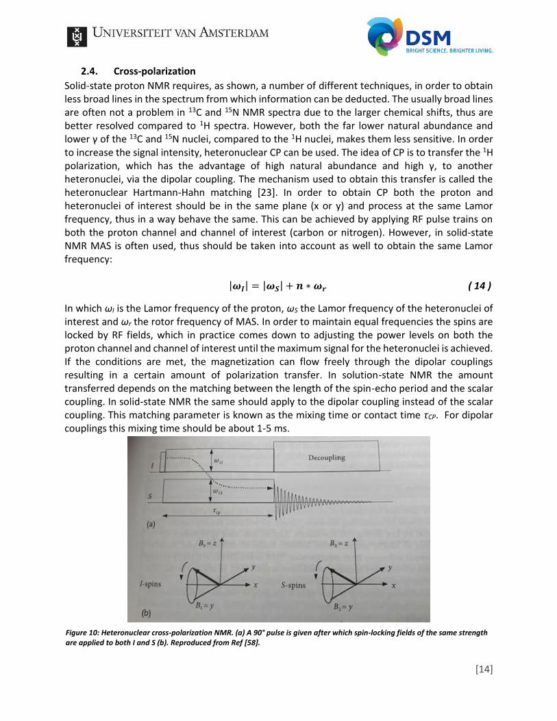
Solid-state proton NMR requires, as shown, a number of different techniques, in order to obtain less broad lines in the spectrum from which information can be deducted. The usually broad lines are often not a problem in 13C and 15N NMR spectra due to the larger chemical shifts, thus are better resolved compared to 1H spectra. However, both the far lower natural abundance and lower γ of the 13C and 15N nuclei, compared to the 1H nuclei, makes them less sensitive. In order to increase the signal intensity, heteronuclear CP can be used. The idea of CP is to transfer the 1H polarization, which has the advantage of high natural abundance and high γ, to another heteronuclei, via the dipolar coupling. The mechanism used to obtain this transfer is called the heteronuclear Hartmann-Hahn matching [23]. In order to obtain CP both the proton and heteronuclei of interest should be in the same plane (x or y) and process at the same Lamor frequency, thus in a way behave the same. This can be achieved by applying RF pulse trains on both the proton channel and channel of interest (carbon or nitrogen). However, in solid-state NMR MAS is often used, thus should be taken into account as well to obtain the same Lamor frequency: |𝝎𝑰| = |𝝎𝑺| + 𝒏 ∗ 𝝎𝒓 ( 14 )

In which ωI is the Lamor frequency of the proton, ωS the Lamor frequency of the heteronuclei of interest and ωr the rotor frequency of MAS. In order to maintain equal frequencies the spins are locked by RF fields, which in practice comes down to adjusting the power levels on both the proton channel and channel of interest until the maximum signal for the heteronuclei is achieved. If the conditions are met, the magnetization can flow freely through the dipolar couplings resulting in a certain amount of polarization transfer. In solution-state NMR the amount transferred depends on the matching between the length of the spin-echo period and the scalar coupling. In solid-state NMR the same should apply to the dipolar coupling instead of the scalar coupling. This matching parameter is known as the mixing time or contact time τCP. For dipolar couplings this mixing time should be about 1-5 ms.

Figure 10: Heteronuclear cross-polarization NMR. (a) A 90° pulse is given after which spin-locking fields of the same strength are applied to both I and S (b). Reproduced from Ref [58].

[15]

2.5. Multidimensional NMR

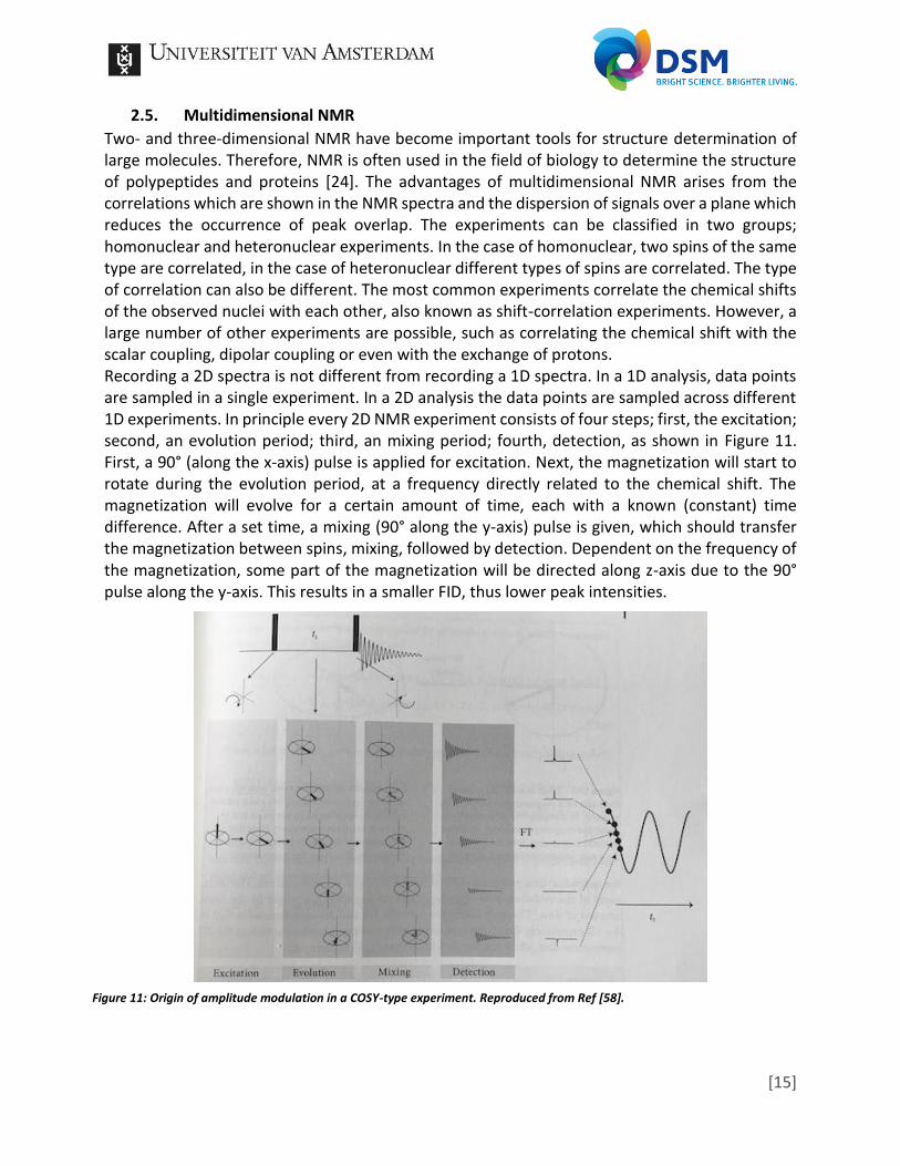
Two- and three-dimensional NMR have become important tools for structure determination of large molecules. Therefore, NMR is often used in the field of biology to determine the structure of polypeptides and proteins [24]. The advantages of multidimensional NMR arises from the correlations which are shown in the NMR spectra and the dispersion of signals over a plane which reduces the occurrence of peak overlap. The experiments can be classified in two groups; homonuclear and heteronuclear experiments. In the case of homonuclear, two spins of the same type are correlated, in the case of heteronuclear different types of spins are correlated. The type of correlation can also be different. The most common experiments correlate the chemical shifts of the observed nuclei with each other, also known as shift-correlation experiments. However, a large number of other experiments are possible, such as correlating the chemical shift with the scalar coupling, dipolar coupling or even with the exchange of protons. Recording a 2D spectra is not different from recording a 1D spectra. In a 1D analysis, data points are sampled in a single experiment. In a 2D analysis the data points are sampled across different 1D experiments. In principle every 2D NMR experiment consists of four steps; first, the excitation; second, an evolution period; third, an mixing period; fourth, detection, as shown in Figure 11. First, a 90° (along the x-axis) pulse is applied for excitation. Next, the magnetization will start to rotate during the evolution period, at a frequency directly related to the chemical shift. The magnetization will evolve for a certain amount of time, each with a known (constant) time difference. After a set time, a mixing (90° along the y-axis) pulse is given, which should transfer the magnetization between spins, mixing, followed by detection. Dependent on the frequency of the magnetization, some part of the magnetization will be directed along z-axis due to the 90° pulse along the y-axis. This results in a smaller FID, thus lower peak intensities.

Figure 11: Origin of amplitude modulation in a COSY-type experiment. Reproduced from Ref [58].

[16]

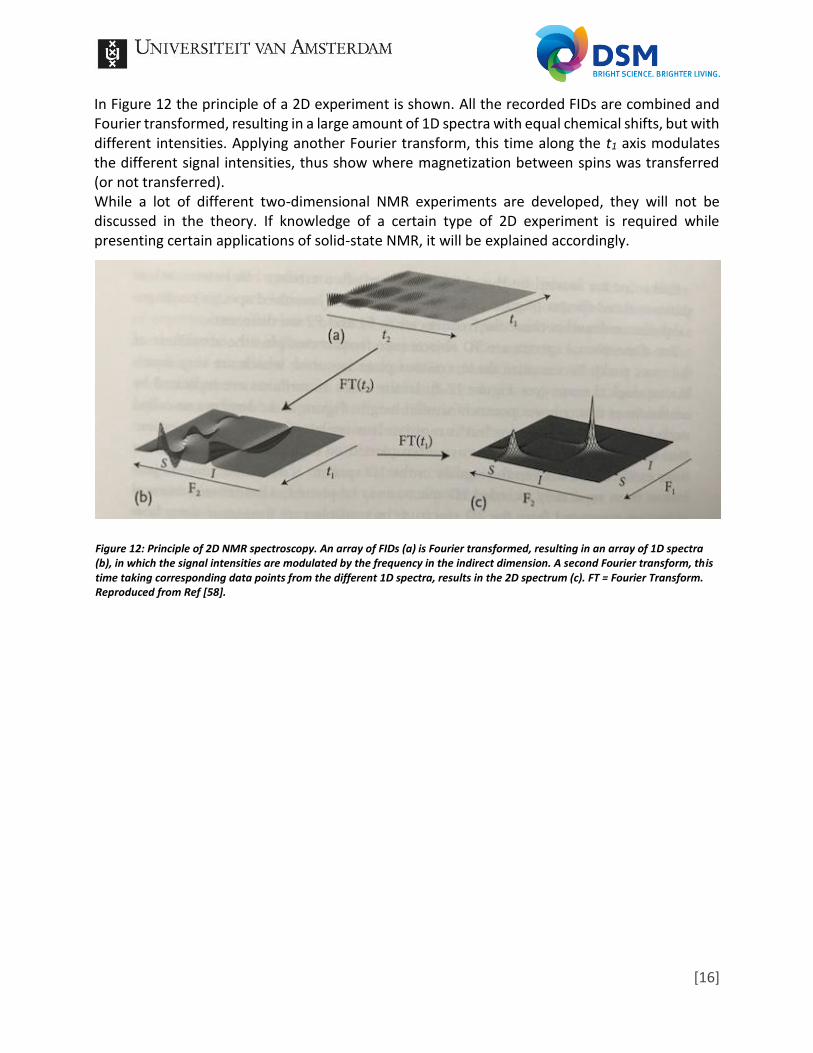
In Figure 12 the principle of a 2D experiment is shown. All the recorded FIDs are combined and Fourier transformed, resulting in a large amount of 1D spectra with equal chemical shifts, but with different intensities. Applying another Fourier transform, this time along the t1 axis modulates the different signal intensities, thus show where magnetization between spins was transferred (or not transferred). While a lot of different two-dimensional NMR experiments are developed, they will not be discussed in the theory. If knowledge of a certain type of 2D experiment is required while presenting certain applications of solid-state NMR, it will be explained accordingly.

Figure 12: Principle of 2D NMR spectroscopy. An array of FIDs (a) is Fourier transformed, resulting in an array of 1D spectra (b), in which the signal intensities are modulated by the frequency in the indirect dimension. A second Fourier transform, this time taking corresponding data points from the different 1D spectra, results in the 2D spectrum (c). FT = Fourier Transform. Reproduced from Ref [58].

[17]

3. Applications In this chapter certain applications will be described which either focus on solid-state NMR polymer analysis, high resolution 1H solid-state NMR or a combination of both.

3.1. Morphology by 13C solid-state NMR

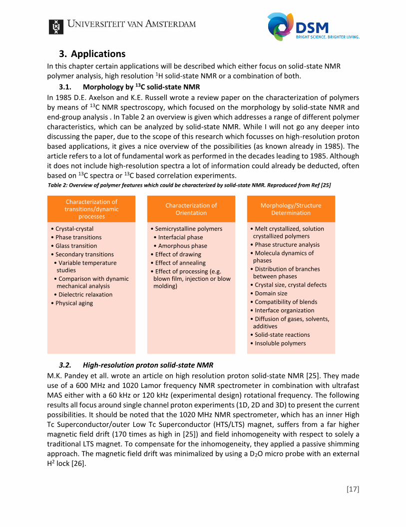
In 1985 D.E. Axelson and K.E. Russell wrote a review paper on the characterization of polymers by means of 13C NMR spectroscopy, which focused on the morphology by solid-state NMR and end-group analysis . In Table 2 an overview is given which addresses a range of different polymer characteristics, which can be analyzed by solid-state NMR. While I will not go any deeper into discussing the paper, due to the scope of this research which focusses on high-resolution proton based applications, it gives a nice overview of the possibilities (as known already in 1985). The article refers to a lot of fundamental work as performed in the decades leading to 1985. Although it does not include high-resolution spectra a lot of information could already be deducted, often based on 13C spectra or 13C based correlation experiments.

3.2. High-resolution proton solid-state NMR

M.K. Pandey et all. wrote an article on high resolution proton solid-state NMR [25]. They made use of a 600 MHz and 1020 Lamor frequency NMR spectrometer in combination with ultrafast MAS either with a 60 kHz or 120 kHz (experimental design) rotational frequency. The following results all focus around single channel proton experiments (1D, 2D and 3D) to present the current possibilities. It should be noted that the 1020 MHz NMR spectrometer, which has an inner High Tc Superconductor/outer Low Tc Superconductor (HTS/LTS) magnet, suffers from a far higher magnetic field drift (170 times as high in [25]) and field inhomogeneity with respect to solely a traditional LTS magnet. To compensate for the inhomogeneity, they applied a passive shimming approach. The magnetic field drift was minimalized by using a D2O micro probe with an external H2 lock [26].

Characterization of transitions/dynamic

processes

• Crystal-crystal

• Phase transitions

• Glass transition

• Secondary transitions

• Variable temperature studies

• Comparison with dynamic mechanical analysis

• Dielectric relaxation

• Physical aging

Characterization of Orientation

• Semicrystalline polymers

• Interfacial phase

• Amorphous phase

• Effect of drawing

• Effect of annealing

• Effect of processing (e.g. blown film, injection or blow molding)

Morphology/Structure Determination

• Melt crystallized, solution crystallized polymers

• Phase structure analysis

• Molecula dynamics of phases

• Distribution of branches between phases

• Crystal size, crystal defects

• Domain size

• Compatibility of blends

• Interface organization

• Diffusion of gases, solvents, additives

• Solid-state reactions

• Insoluble polymers

Table 2: Overview of polymer features which could be characterized by solid-state NMR. Reproduced from Ref [25]

[18]

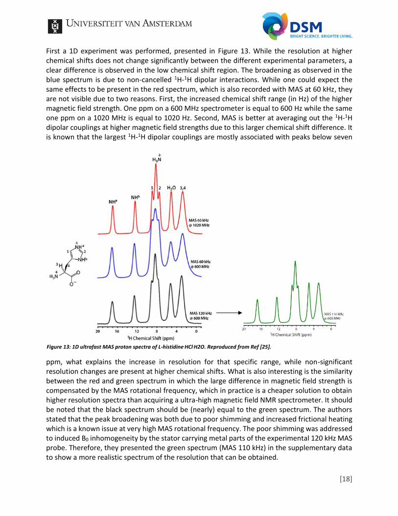
First a 1D experiment was performed, presented in Figure 13. While the resolution at higher chemical shifts does not change significantly between the different experimental parameters, a clear difference is observed in the low chemical shift region. The broadening as observed in the blue spectrum is due to non-cancelled 1H-1H dipolar interactions. While one could expect the same effects to be present in the red spectrum, which is also recorded with MAS at 60 kHz, they are not visible due to two reasons. First, the increased chemical shift range (in Hz) of the higher magnetic field strength. One ppm on a 600 MHz spectrometer is equal to 600 Hz while the same one ppm on a 1020 MHz is equal to 1020 Hz. Second, MAS is better at averaging out the 1H-1H dipolar couplings at higher magnetic field strengths due to this larger chemical shift difference. It is known that the largest 1H-1H dipolar couplings are mostly associated with peaks below seven

ppm, what explains the increase in resolution for that specific range, while non-significant resolution changes are present at higher chemical shifts. What is also interesting is the similarity between the red and green spectrum in which the large difference in magnetic field strength is compensated by the MAS rotational frequency, which in practice is a cheaper solution to obtain higher resolution spectra than acquiring a ultra-high magnetic field NMR spectrometer. It should be noted that the black spectrum should be (nearly) equal to the green spectrum. The authors stated that the peak broadening was both due to poor shimming and increased frictional heating which is a known issue at very high MAS rotational frequency. The poor shimming was addressed to induced B0 inhomogeneity by the stator carrying metal parts of the experimental 120 kHz MAS probe. Therefore, they presented the green spectrum (MAS 110 kHz) in the supplementary data to show a more realistic spectrum of the resolution that can be obtained.

Figure 13: 1D ultrafast MAS proton spectra of L-histidine.HCl.H2O. Reproduced from Ref [25].

[19]

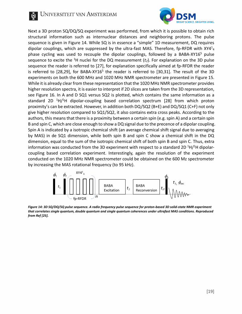
Next a 3D proton SQ/DQ/SQ experiment was performed, from which it is possible to obtain rich structural information such as internuclear distances and neighboring protons. The pulse sequence is given in Figure 14. While SQ is in essence a “simple” 1D measurement, DQ requires dipolar couplings, which are suppressed by the ultra-fast MAS. Therefore, fp-RFDR with XY41

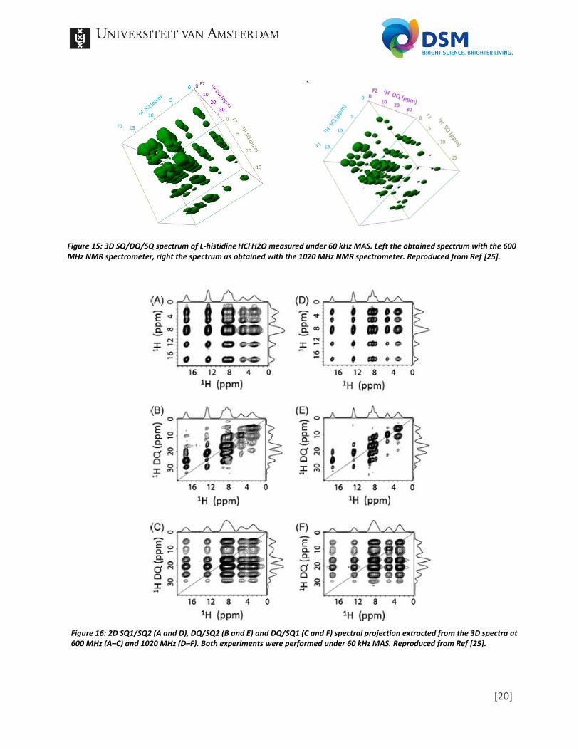
4 phase cycling was used to recouple the dipolar couplings, followed by a BABA-XY165 pulse sequence to excite the 1H nuclei for the DQ measurement (t2). For explanation on the 3D pulse sequence the reader is referred to [27], for explanation specifically aimed at fp-RFDR the reader is referred to [28,29], for BABA-XY165 the reader is referred to [30,31]. The result of the 3D experiments on both the 600 MHz and 1020 MHz NMR spectrometer are presented in Figure 15. While it is already clear from these representation that the 1020 MHz NMR spectrometer provides higher resolution spectra, it is easier to interpret if 2D slices are taken from the 3D representation, see Figure 16. In A and D SQ1 versus SQ2 is plotted, which contains the same information as a standard 2D 1H/1H dipolar-coupling based correlation spectrum [28] from which proton proximity’s can be extracted. However, in addition both DQ/SQ2 (B+E) and DQ/SQ1 (C+F) not only give higher resolution compared to SQ1/SQ2, it also contains extra cross peaks. According to the authors, this means that there is a proximity between a certain spin (e.g. spin A) and a certain spin B and spin C, which are close enough to show a DQ signal due to the precence of a dipolar coupling. Spin A is indicated by a isotropic chemical shift (an average chemical shift signal due to averaging by MAS) in de SQ1 dimension, while both spin B and spin C show a chemical shift in the DQ dimension, equal to the sum of the isotropic chemical shift of both spin B and spin C. Thus, extra information was conducted from the 3D experiment with respect to a standard 2D 1H/1H dipolar-coupling based correlation experiment. Interestingly, again the resolution of the experiment conducted on the 1020 MHz NMR spectrometer could be obtained on the 600 Mz spectrometer by increasing the MAS rotational frequency (to 95 kHz).

Figure 14: 3D SQ/DQ/SQ pulse sequence. A radio frequency pulse sequence for proton-based 3D solid-state NMR experiment that correlates single quantum, double quantum and single quantum coherences under ultrafast MAS conditions. Reproduced from Ref [25].

[20]

Figure 15: 3D SQ/DQ/SQ spectrum of L-histidine.HCl.H2O measured under 60 kHz MAS. Left the obtained spectrum with the 600 MHz NMR spectrometer, right the spectrum as obtained with the 1020 MHz NMR spectrometer. Reproduced from Ref [25].

Figure 16: 2D SQ1/SQ2 (A and D), DQ/SQ2 (B and E) and DQ/SQ1 (C and F) spectral projection extracted from the 3D spectra at 600 MHz (A–C) and 1020 MHz (D–F). Both experiments were performed under 60 kHz MAS. Reproduced from Ref [25].

[21]

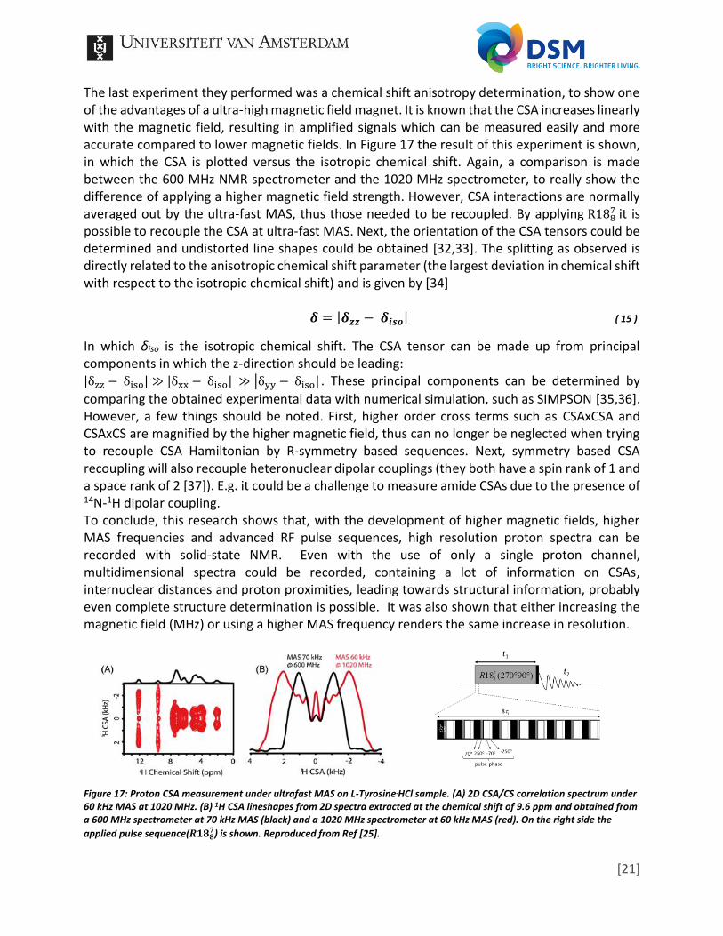
The last experiment they performed was a chemical shift anisotropy determination, to show one of the advantages of a ultra-high magnetic field magnet. It is known that the CSA increases linearly with the magnetic field, resulting in amplified signals which can be measured easily and more accurate compared to lower magnetic fields. In Figure 17 the result of this experiment is shown, in which the CSA is plotted versus the isotropic chemical shift. Again, a comparison is made between the 600 MHz NMR spectrometer and the 1020 MHz spectrometer, to really show the difference of applying a higher magnetic field strength. However, CSA interactions are normally averaged out by the ultra-fast MAS, thus those needed to be recoupled. By applying R188

7 it is possible to recouple the CSA at ultra-fast MAS. Next, the orientation of the CSA tensors could be determined and undistorted line shapes could be obtained [32,33]. The splitting as observed is directly related to the anisotropic chemical shift parameter (the largest deviation in chemical shift with respect to the isotropic chemical shift) and is given by [34] 𝜹 = |𝜹𝒛𝒛 − 𝜹𝒊𝒔𝒐| ( 15 )

In which δiso is the isotropic chemical shift. The CSA tensor can be made up from principal components in which the z-direction should be leading: |δzz − δiso| ≫ |δxx − δiso| ≫ |δyy − δiso| . These principal components can be determined by

comparing the obtained experimental data with numerical simulation, such as SIMPSON [35,36]. However, a few things should be noted. First, higher order cross terms such as CSAxCSA and CSAxCS are magnified by the higher magnetic field, thus can no longer be neglected when trying to recouple CSA Hamiltonian by R-symmetry based sequences. Next, symmetry based CSA recoupling will also recouple heteronuclear dipolar couplings (they both have a spin rank of 1 and a space rank of 2 [37]). E.g. it could be a challenge to measure amide CSAs due to the presence of 14N-1H dipolar coupling. To conclude, this research shows that, with the development of higher magnetic fields, higher MAS frequencies and advanced RF pulse sequences, high resolution proton spectra can be recorded with solid-state NMR. Even with the use of only a single proton channel, multidimensional spectra could be recorded, containing a lot of information on CSAs, internuclear distances and proton proximities, leading towards structural information, probably even complete structure determination is possible. It was also shown that either increasing the magnetic field (MHz) or using a higher MAS frequency renders the same increase in resolution.

Figure 17: Proton CSA measurement under ultrafast MAS on L-Tyrosine.HCl sample. (A) 2D CSA/CS correlation spectrum under 60 kHz MAS at 1020 MHz. (B) 1H CSA lineshapes from 2D spectra extracted at the chemical shift of 9.6 ppm and obtained from a 600 MHz spectrometer at 70 kHz MAS (black) and a 1020 MHz spectrometer at 60 kHz MAS (red). On the right side the

applied pulse sequence(𝑹𝟏𝟖𝟖𝟕) is shown. Reproduced from Ref [25].

[22]

3.3. Protein structure determination

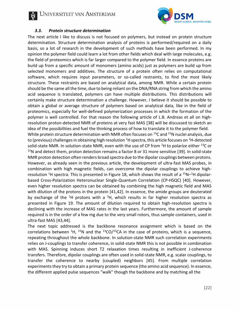
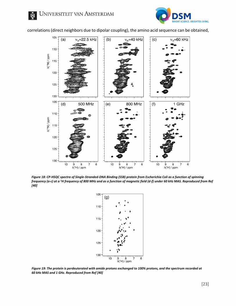
The next article I like to discuss is not focused on polymers, but instead on protein structure determination. Structure determination analysis of proteins is performed/required on a daily basis, so a lot of research in the development of such methods have been performed. In my opinion the polymer field could learn a lot from other fields which deal with large molecules, e.g. the field of proteomics which is far larger compared to the polymer field. In essence proteins are build up from a specific amount of monomers (amino acids) just as polymers are build up from selected monomers and additives. The structure of a protein often relies on computational software, which requires input parameters, or so-called restraints, to find the most likely structure. These restraints are based on analytical data, among NMR. While a certain protein should be the same all the time, due to being reliant on the DNA/RNA string from which the amino acid sequence is translated, polymers can have multiple distributions. This distributions will certainly make structure determination a challenge. However, I believe it should be possible to obtain a global or average structure of polymers based on analytical data, like in the field of proteomics, especially for well-defined polymerization processes in which the formation of the polymer is well controlled. For that reason the following article of L.B. Andreas et all on high-resolution proton-detected NMR of proteins at very fast MAS [38] will be discussed to sketch an idea of the possibilities and fuel the thinking process of how to translate it to the polymer field. While protein structure determination with NMR often focuses on 13C and 15N nuclei analysis, due to (previous) challenges in obtaining high resolution 1H spectra, this article focuses on 1H-detected solid-state NMR. In solution-state NMR, even with the use of CP from 1H to polarize either 13C or 15N and detect them, proton detection remains a factor 8 or 31 more sensitive [39]. In solid-state NMR proton detection often renders broad spectra due to the dipolar couplings between protons. However, as already seen in the previous article, the development of ultra-fast MAS probes, in combination with high magnetic fields, can overcome the dipolar couplings to achieve high-resolution 1H spectra. This is presented in Figure 18, which shows the result of a 15N–1H dipolar-based Cross-Polarization Heteronuclear Single-Quantum Correlation (CP-HSQC) [40]. However, even higher resolution spectra can be obtained by combining the high magnetic field and MAS with dilution of the protons in the protein [41,42]. In essence, the amide groups are deuterated by exchange of the 1H protons with a 2H, which results in far higher resolution spectra as presented in Figure 19. The amount of dilution required to obtain high-resolution spectra is declining with the increase of MAS rates in the last years. Furthermore, the amount of sample required is in the order of a few mg due to the very small rotors, thus sample containers, used in ultra-fast MAS [43,44]. The next topic addressed is the backbone resonance assignment which is based on the correlations between 1H, 15N and the 13CO/13CA in the case of proteins, which is a sequence, repeating throughout the whole backbone. In solution-state NMR such correlation experiments relies on J-couplings to transfer coherence, in solid-state NMR this is not possible in combination with MAS. Spinning induces short T2 relaxation times resulting in inefficient J-coherence transfers. Therefore, dipolar couplings are often used in solid-state NMR, e.g. scalar couplings, to transfer the coherence to nearby (coupled) neighbors [45]. From multiple correlation experiments they try to obtain a primary protein sequence (the amino acid sequence). In essence, the different applied pulse sequences “walk” though the backbone and by matching all the

[23]

correlations (direct neighbors due to dipolar coupling), the amino acid sequence can be obtained,

Figure 18: CP-HSQC spectra of Single-Stranded-DNA Binding (SSB) protein from Escherichia Coli as a function of spinning frequency (a-c) at a 1H frequency of 800 MHz and as a function of magnetic field (d-f) under 60 kHz MAS. Reproduced from Ref [40]

Figure 19: The protein is perdeuterated with amide protons exchanged to 100% protons, and the spectrum recorded at 60 kHz MAS and 1 GHz. Reproduced from Ref [40]

[24]

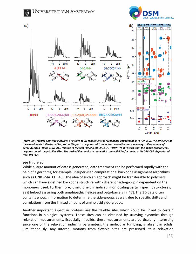
see Figure 20. While a large amount of data is generated, data treatment can be performed rapidly with the

help of algorithms, for example unsupervised computational backbone assignment algorithms

such as UNIO-MATCH [46]. The idea of such an approach might be transferable to polymers

which can have a defined backbone structure with different “side-groups” dependent on the

monomers used. Furthermore, it might help in indicating or locating certain specific structures,

as it helped assigning both amphipathic helices and beta-barrels in [47]. The 3D data often

contains enough information to determine the side-groups as well, due to specific shifts and

correlations from the limited amount of amino acid side-groups.

Another important aspect in proteins are the flexible sites which could be linked to certain functions in biological systems. These sites can be obtained by studying dynamics through relaxation measurements. Especially in solids, these measurements are particularly interesting since one of the relaxation inducing parameters, the molecular tumbling, is absent in solids. Simultaneously, any internal motions from flexible sites are preserved, thus relaxation

Figure 20: Transfer pathway diagrams of a suite of 3D experiments for resonance assignment as in Ref. [59]. The efficiency of the experiments is illustrated by proton 1D spectra acquired with no indirect evolutions on a microcrystalline sample of perdeuterated [100%-1HN] SH3, relative to the first FID of a 2D CP-HSQC (‘‘(H)NH’’). (b) Strips from the above experiments, acquired on microcrystalline β2m. The dashed lines indicate sequential connectivities for amino acids D76-C80. Reproduced from Ref [47].

[25]

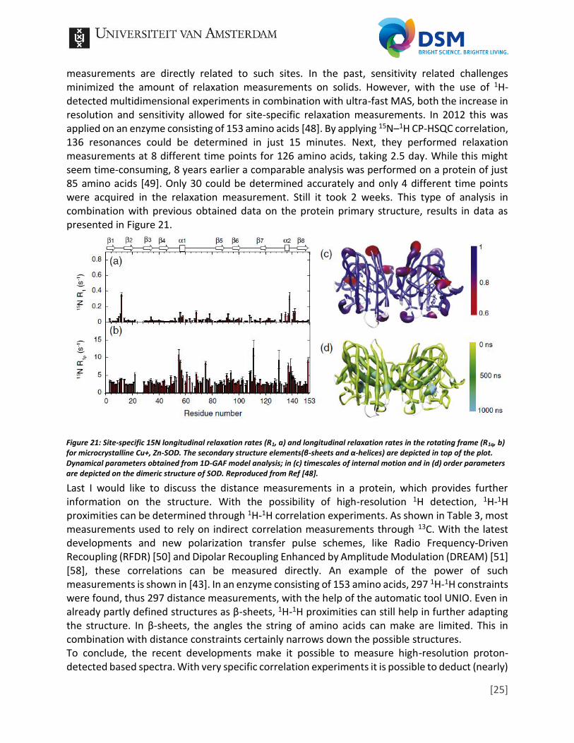
measurements are directly related to such sites. In the past, sensitivity related challenges minimized the amount of relaxation measurements on solids. However, with the use of 1H-detected multidimensional experiments in combination with ultra-fast MAS, both the increase in resolution and sensitivity allowed for site-specific relaxation measurements. In 2012 this was applied on an enzyme consisting of 153 amino acids [48]. By applying 15N–1H CP-HSQC correlation, 136 resonances could be determined in just 15 minutes. Next, they performed relaxation measurements at 8 different time points for 126 amino acids, taking 2.5 day. While this might seem time-consuming, 8 years earlier a comparable analysis was performed on a protein of just 85 amino acids [49]. Only 30 could be determined accurately and only 4 different time points were acquired in the relaxation measurement. Still it took 2 weeks. This type of analysis in combination with previous obtained data on the protein primary structure, results in data as presented in Figure 21.

Last I would like to discuss the distance measurements in a protein, which provides further information on the structure. With the possibility of high-resolution 1H detection, 1H-1H proximities can be determined through 1H-1H correlation experiments. As shown in Table 3, most measurements used to rely on indirect correlation measurements through 13C. With the latest developments and new polarization transfer pulse schemes, like Radio Frequency-Driven Recoupling (RFDR) [50] and Dipolar Recoupling Enhanced by Amplitude Modulation (DREAM) [51] [58], these correlations can be measured directly. An example of the power of such measurements is shown in [43]. In an enzyme consisting of 153 amino acids, 297 1H-1H constraints were found, thus 297 distance measurements, with the help of the automatic tool UNIO. Even in already partly defined structures as β-sheets, 1H-1H proximities can still help in further adapting the structure. In β-sheets, the angles the string of amino acids can make are limited. This in combination with distance constraints certainly narrows down the possible structures. To conclude, the recent developments make it possible to measure high-resolution proton-detected based spectra. With very specific correlation experiments it is possible to deduct (nearly)

Figure 21: Site-specific 15N longitudinal relaxation rates (R1, a) and longitudinal relaxation rates in the rotating frame (R1q, b) for microcrystalline Cu+, Zn-SOD. The secondary structure elements(β-sheets and α-helices) are depicted in top of the plot. Dynamical parameters obtained from 1D-GAF model analysis; in (c) timescales of internal motion and in (d) order parameters are depicted on the dimeric structure of SOD. Reproduced from Ref [48].

[26]

the whole protein structure by obtaining the primary sequence in combination with multiple constraints on their 3D structure order. Furthermore, relaxation experiment can provide insight in flexible sites within the protein, which can indicate the possible location(s) of active sites, involved in biological processes.

3.4. Hydrogen bond interaction and dynamics in polymer blends

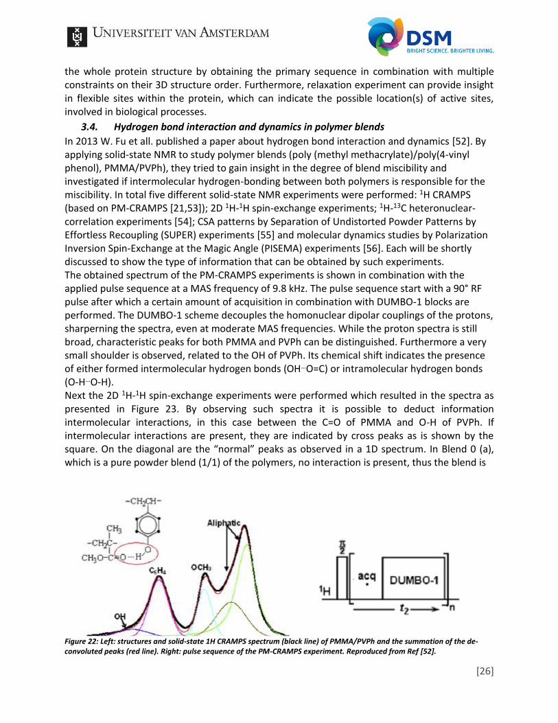
In 2013 W. Fu et all. published a paper about hydrogen bond interaction and dynamics [52]. By applying solid-state NMR to study polymer blends (poly (methyl methacrylate)/poly(4-vinyl phenol), PMMA/PVPh), they tried to gain insight in the degree of blend miscibility and investigated if intermolecular hydrogen-bonding between both polymers is responsible for the miscibility. In total five different solid-state NMR experiments were performed: 1H CRAMPS (based on PM-CRAMPS [21,53]); 2D 1H-1H spin-exchange experiments; 1H-13C heteronuclear-correlation experiments [54]; CSA patterns by Separation of Undistorted Powder Patterns by Effortless Recoupling (SUPER) experiments [55] and molecular dynamics studies by Polarization Inversion Spin-Exchange at the Magic Angle (PISEMA) experiments [56]. Each will be shortly discussed to show the type of information that can be obtained by such experiments. The obtained spectrum of the PM-CRAMPS experiments is shown in combination with the applied pulse sequence at a MAS frequency of 9.8 kHz. The pulse sequence start with a 90° RF pulse after which a certain amount of acquisition in combination with DUMBO-1 blocks are performed. The DUMBO-1 scheme decouples the homonuclear dipolar couplings of the protons, sharperning the spectra, even at moderate MAS frequencies. While the proton spectra is still broad, characteristic peaks for both PMMA and PVPh can be distinguished. Furthermore a very small shoulder is observed, related to the OH of PVPh. Its chemical shift indicates the presence of either formed intermolecular hydrogen bonds (OH…O=C) or intramolecular hydrogen bonds (O-H…O-H). Next the 2D 1H-1H spin-exchange experiments were performed which resulted in the spectra as presented in Figure 23. By observing such spectra it is possible to deduct information intermolecular interactions, in this case between the C=O of PMMA and O-H of PVPh. If intermolecular interactions are present, they are indicated by cross peaks as is shown by the square. On the diagonal are the “normal” peaks as observed in a 1D spectrum. In Blend 0 (a), which is a pure powder blend (1/1) of the polymers, no interaction is present, thus the blend is

Figure 22: Left: structures and solid-state 1H CRAMPS spectrum (black line) of PMMA/PVPh and the summation of the de-convoluted peaks (red line). Right: pulse sequence of the PM-CRAMPS experiment. Reproduced from Ref [52].

[27]

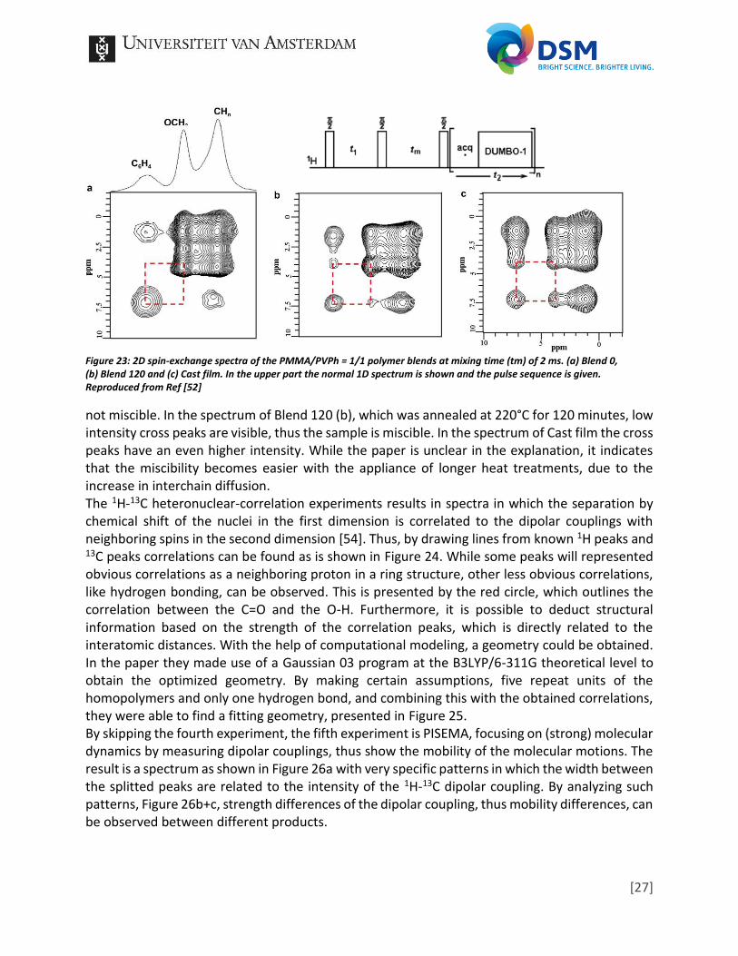
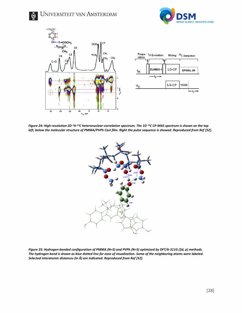
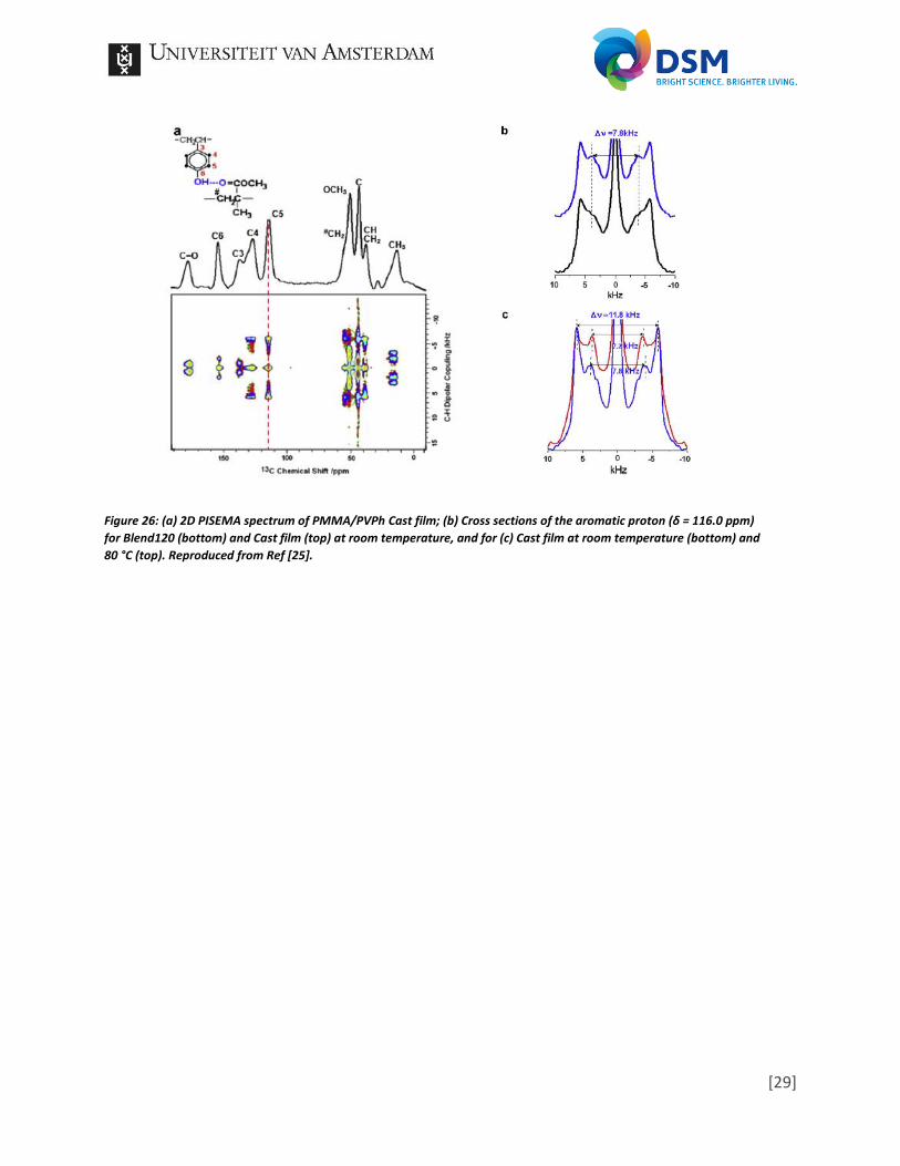
not miscible. In the spectrum of Blend 120 (b), which was annealed at 220°C for 120 minutes, low intensity cross peaks are visible, thus the sample is miscible. In the spectrum of Cast film the cross peaks have an even higher intensity. While the paper is unclear in the explanation, it indicates that the miscibility becomes easier with the appliance of longer heat treatments, due to the increase in interchain diffusion. The 1H-13C heteronuclear-correlation experiments results in spectra in which the separation by chemical shift of the nuclei in the first dimension is correlated to the dipolar couplings with neighboring spins in the second dimension [54]. Thus, by drawing lines from known 1H peaks and 13C peaks correlations can be found as is shown in Figure 24. While some peaks will represented obvious correlations as a neighboring proton in a ring structure, other less obvious correlations, like hydrogen bonding, can be observed. This is presented by the red circle, which outlines the correlation between the C=O and the O-H. Furthermore, it is possible to deduct structural information based on the strength of the correlation peaks, which is directly related to the interatomic distances. With the help of computational modeling, a geometry could be obtained. In the paper they made use of a Gaussian 03 program at the B3LYP/6-311G theoretical level to obtain the optimized geometry. By making certain assumptions, five repeat units of the homopolymers and only one hydrogen bond, and combining this with the obtained correlations, they were able to find a fitting geometry, presented in Figure 25. By skipping the fourth experiment, the fifth experiment is PISEMA, focusing on (strong) molecular dynamics by measuring dipolar couplings, thus show the mobility of the molecular motions. The result is a spectrum as shown in Figure 26a with very specific patterns in which the width between the splitted peaks are related to the intensity of the 1H-13C dipolar coupling. By analyzing such patterns, Figure 26b+c, strength differences of the dipolar coupling, thus mobility differences, can be observed between different products.

Figure 23: 2D spin-exchange spectra of the PMMA/PVPh = 1/1 polymer blends at mixing time (tm) of 2 ms. (a) Blend 0, (b) Blend 120 and (c) Cast film. In the upper part the normal 1D spectrum is shown and the pulse sequence is given. Reproduced from Ref [52]

[28]

Figure 24: High-resolution 2D 1H-13C heteronuclear-correlation spectrum. The 1D 13C CP-MAS spectrum is shown on the top left, below the molecular structure of PMMA/PVPh Cast film. Right the pulse sequence is showed. Reproduced from Ref [52].

Figure 25: Hydrogen-bonded configuration of PMMA (N=5) and PVPh (N=5) optimized by DFT/6-311G (2d, p) methods. The hydrogen bond is drawn as blue dotted line for ease of visualization. Some of the neighboring atoms were labeled. Selected interatomic distances (in Å) are indicated. Reproduced from Ref [52].

[29]

Figure 26: (a) 2D PISEMA spectrum of PMMA/PVPh Cast film; (b) Cross sections of the aromatic proton (δ = 116.0 ppm)

for Blend120 (bottom) and Cast film (top) at room temperature, and for (c) Cast film at room temperature (bottom) and

80 °C (top). Reproduced from Ref [25].

[30]

4. Conclusion/summary In this literature thesis multiple aspect of solid-state NMR were addressed in combination with some of the latest applications, mostly focused around proton-detected solid-state NMR. While dipolar interactions used to result in broad spectra, the latest developments in high magnetic fields helped to increase the resolution. However, more importantly for the increase in resolution were the developments of ultra-fast MAS probes, combined with RF pulse sequences and the adaption of such pulse sequences to the ultra-fast MAS. The availability of high-resolution 1H spectra has increased the amount of applications in solid-state NMR with relation to correlation experiments. While most correlation experiments focused around 13C and 15N, their sensitivity due to lower natural abundance and gyromagnetic ratio is lower compared to 1H. Furthermore, 1H is often largely abundant in most studied samples as polymers and proteins, thus can provide further inside in both the structure and the dynamics of the sample of interest. In this research the results were shown of high-resolution proton solid-state NMR by using single proton channel detection. The results proved that it was possible to obtain high-resolution 1D, 2D and 3D proton spectra in combination with ultra-fast MAS. The 3D correlation spectra even showed new cross-peaks, which would be missed with 2D correlation experiments. Besides correlation experiments, the possibility to perform highly accurate CSA measurements was also shown. Both the proton correlation experiments as the CSAs determination can provide structural information. Next the results of high-resolution proton solid-state NMR in the analysis of proteins were presented. Proteins share certain relations with polymers, which makes it an interesting field to learn from. Examples were shown of certain steps involved in the structure elucidation of proteins. The use of multiple 3D correlation experiments on the typical protein backbone in combination with unsupervised computational backbone assignment algorithms resulted in (partly) solved amino-acid sequences (primary structure). After assignment of the backbone, 1H-1H correlations were determined, from which internuclear distances could be calculated of the dipolar interactions. These distances than provide restrictions on the structure determination. With enough restrictions the number of possible structures drops dramatically, to eventually obtain the most likely structure for a certain protein. Furthermore, it is possible to dynamic processes, which could indicate the active sides in the protein, involved in certain processes. Last the results of the same type of experiments, but on a polymer blend of PMMA/PVPh were presented, with the focus on hydrogen bonding interactions, which were expected to influence the miscibility. Hydrogen bonding interactions was observed in multiple correlation experiments, both homonuclear and heteronuclear. Again calculated internuclear distances provided restrictions from which by numerical methods a possible structure of the blend with the hydrogen bonding could be determined. CSAs of specific peaks from the polymer blend spectrum were also determined. All together solid-state NMR has come a far way in the last decades. Especially around 2015 a jump in high-resolution proton spectra is visible, together with very impressive applications, due to the availability of ultra-fast MAS (> 100 kHz) and pulse sequences which can deal with such high MAS frequencies. In essence, especially the capability of obtaining high resolution

[31]

correlation spectra, either heteronuclear or homonuclear, allows for important applications. I certainly expect that the upcoming decade should provide us with a large amount of newly obtained data on solid samples, pushing both our knowledge on the structural information as well as their influence on certain applications.

[32]

5. Literature

[1] F. Bloch, W.W. Hansen, M. Packard, Nuclear Induction, Phys. Rev. 69 (1946) 127. doi:10.1103/PhysRev.69.127.

[2] E. Purcell, H. Torrey, R. Pound, Resonance Absorption by Nuclear Magnetic Moments in a Solid, Phys. Rev. 69 (1946) 37–38. doi:10.1103/PhysRev.69.37.

[3] N. Bloembergen, E.M. Purcell, R. V. Pound, Relaxation Effects in Nuclear in Nuclear Magnetic Resonance Absorption, Phys. Rev. 73 (1948) 679. doi:10.1103/PhysRev.73.679.

[4] H.S. Gutowsky, D.W. McCall, Nuclear Magnetic Resonance Fine Structure in Liquids, Phys. Rev. 82 (1951) 748–749. doi:https://doi.org/10.1103/PhysRev.82.748.

[5] F. Bloch, Nuclear Induction, Phys. Rev. 70 (1946) 460. doi:https://doi.org/10.1103/PhysRev.70.460.

[6] E.L. Hahn, An Accurate Nuclear Magnetic Resonance Method for Measuring Spin-Lattice Relaxation Times, Phys. Rev. 76 (1949) 145.

[7] E.L. Hahn, Spin Echoes, Phys. Rev. 80 (1950) 580.

[8] K. Saalwächter, D. Reichert, Polymer Applications of NMR, in: Encycl. Spectrosc. Spectrom., 2010: pp. 2221–2236. doi:10.1016/B978-0-12-374413-5.00032-4.

[9] S. Ablett, Overview of NMR applications in food science, Trends Food Sci. Technol. 3 (1992) 246–250. doi:10.1016/S0924-2244(10)80002-0.

[10] J.C. Lindon, Overview of NMR-Based Metabonomics, in: Encycl. Spectrosc. Spectrom., 2010: pp. 2058–2068. doi:10.1016/B978-0-12-374413-5.00078-6.

[11] M.E. Halse, L. Emsley, A common theory for phase-modulated homonuclear decoupling in solid-state NMR, Phys. Chem. Chem. Phys. 14 (2012) 9121–9130. doi:10.1039/C2CP40720E.

[12] K.R. Mote, V. Agarwal, P.K. Madhu, Five decades of homonuclear dipolar decoupling in solid-state NMR: Status and outlook, Prog. Nucl. Magn. Reson. Spectrosc. 97 (2016) 1–39. doi:10.1016/j.pnmrs.2016.08.001.

[13] Y. Nishiyama, Fast magic-angle sample spinning solid-state NMR at 60–100 kHz for natural abundance samples, Solid State Nucl. Magn. Reson. 78 (2016) 24–36. doi:10.1016/j.ssnmr.2016.06.002.

[14] Y. Endo, K. Hioka, K. Yamauchi, Sample Tube and Measurement Method for Solid-state NMR, US Patent., 8,436,616 (n.d.).

[15] A.L. Bloom, J.N. Shoolery, Effects of perturbing radiofrequency fields on nuclear spin coupling, Phys. Rev. 97 (1955) 1261–1265. doi:10.1103/PhysRev.97.1261.

[16] M. Lee, W.I. Goldburg, Nuclear-magnetic-resonance line narrowing by a rotating rf field, Phys. Rev. 140 (1965). doi:10.1103/PhysRev.140.A1261.

[17] E. Vinogradov, P.K. Madhu, S. Vega, High-resolution proton solid-state NMR spectroscopy by phase-modulated Lee–Goldburg experiment, Chem. Phys. Lett. 314 (1999) 443–450. doi:10.1016/S0009-2614(99)01174-4.

[33]

[18] M. Leskes, P.K. Madhu, S. Vega, Floquet theory in solid-state nuclear magnetic resonance, Prog. Nucl. Magn. Reson. Spectrosc. 57 (2010) 345–380. doi:10.1016/j.pnmrs.2010.06.002.

[19] E. Vinogradov, P.K. Madhu, S. Vega, Proton spectroscopy in solid state nuclear magnetic resonance with windowed phase modulated Lee-Goldburg decoupling sequences, Chem. Phys. Lett. 354 (2002) 193–202. doi:10.1016/S0009-2614(02)00060-X.

[20] D. Sakellariou, A. Lesage, P. Hodgkinson, L. Emsley, Homonuclear dipolar decoupling in solid-state NMR using continuous phase modulation, Chem. Phys. Lett. 319 (2000) 253–260. doi:10.1016/S0009-2614(00)00127-5.

[21] B. Elena, G. de Paëpe, L. Emsley, Direct spectral optimisation of proton-proton homonuclear dipolar decoupling in solid-state NMR, Chem. Phys. Lett. 398 (2004) 532–538. doi:10.1016/j.cplett.2004.09.122.

[22] E. Salager, J.N. Dumez, R.S. Stein, S. Steuernagel, A. Lesage, B. Elena-Herrmann, L. Emsley, Homonuclear dipolar decoupling with very large scaling factors for high-resolution ultrafast magic angle spinning 1H solid-state NMR spectroscopy, Chem. Phys. Lett. 498 (2010) 214–220. doi:10.1016/j.cplett.2010.08.038.

[23] S.R. Hartmann, E.L. Hahn, Nuclear double resonance in the rotating frame, Phys. Rev. 128 (1962) 2042–2053. doi:10.1103/PhysRev.128.2042.

[24] H.R. Kalbitzer, K.P. Neidig, W. Hengstenberg, Structure determination of polypeptides and proteins by two-dimensional nuclear magnetic resonance spectroscopy, Phys. B Phys. Condens. Matter. 164 (1990) 180–192. doi:10.1016/0921-4526(90)90074-5.

[25] M.K. Pandey, R. Zhang, K. Hashi, S. Ohki, G. Nishijima, S. Matsumoto, T. Noguchi, K. Deguchi, A. Goto, T. Shimizu, H. Maeda, M. Takahashi, Y. Yanagisawa, T. Yamazaki, S. Iguchi, R. Tanaka, T. Nemoto, T. Miyamoto, H. Suematsu, K. Saito, T. Miki, A. Ramamoorthy, Y. Nishiyama, 1020 MHz single-channel proton fast magic angle spinning solid-state NMR spectroscopy, J. Magn. Reson. 261 (2015) 1–5. doi:10.1016/j.jmr.2015.10.003.

[26] K. Hashi, S. Ohki, S. Matsumoto, G. Nishijima, A. Goto, K. Deguchi, K. Yamada, T. Noguchi, S. Sakai, M. Takahashi, Y. Yanagisawa, S. Iguchi, T. Yamazaki, H. Maeda, R. Tanaka, T. Nemoto, H. Suematsu, T. Miki, K. Saito, T. Shimizu, Achievement of 1020 MHz NMR, J. Magn. Reson. 256 (2015) 30–33. doi:10.1016/j.jmr.2015.04.009.

[27] R. Zhang, M.K. Pandey, Y. Nishiyama, A. Ramamoorthy, A Novel High-Resolution and Sensitivity-Enhanced Three-Dimensional Solid-State NMR Experiment Under Ultrafast Magic Angle Spinning Conditions., Sci. Rep. 5 (2015) 11810. doi:10.1038/srep11810.

[28] Y. Nishiyama, R. Zhang, A. Ramamoorthy, Finite-pulse radio frequency driven recoupling with phase cycling for 2D 1H/1H correlation at ultrafast MAS frequencies, J. Magn. Reson. 243 (2014) 25–32. doi:10.1016/j.jmr.2014.03.004.

[29] R. Zhang, Y. Nishiyama, P. Sun, A. Ramamoorthy, Phase cycling schemes for finite-pulse-RFDR MAS solid state NMR experiments, J. Magn. Reson. 252 (2015) 55–66. doi:10.1016/j.jmr.2014.12.010.

[34]

[30] M. Feike, D.E. Demco, R. Graf, J. Gottwald, S. Hafner, H.W. Spiess, Broadband Multiple-Quantum NMR Spectroscopy, J. Magn. Reson. Ser. A. 122 (1996) 214–221. doi:10.1007/s13398-014-0173-7.2.

[31] K. Saalwächter, F. Lange, K. Matyjaszewski, C.F. Huang, R. Graf, BaBa-xy16: Robust and broadband homonuclear DQ recoupling for applications in rigid and soft solids up to the highest MAS frequencies, J. Magn. Reson. 212 (2011) 204–215. doi:10.1016/j.jmr.2011.07.001.

[32] M.K. Pandey, M. Malon, A. Ramamoorthy, Y. Nishiyama, Composite-180?? pulse-based symmetry sequences to recouple proton chemical shift anisotropy tensors under ultrafast MAS solid-state NMR spectroscopy, J. Magn. Reson. 250 (2015) 45–54. doi:10.1016/j.jmr.2014.11.002.

[33] M.K. Pandey, Y. Nishiyama, Determination of relative orientation between 1H CSA tensors from a 3D solid-state NMR experiment mediated through 1H/1H RFDR mixing under ultrafast MAS, Solid State Nucl. Magn. Reson. 70 (2015) 15–20. doi:10.1016/j.ssnmr.2015.05.001.

[34] H.K. Miah, D.A. Bennett, D. Iuga, J.J. Titman, Measuring proton shift tensors with ultrafast MAS NMR, J. Magn. Reson. 235 (2013) 1–5. doi:10.1016/j.jmr.2013.07.005.

[35] Z. Tošner, R. Andersen, B. Stevensson, M. Edén, N.C. Nielsen, T. Vosegaard, Computer-intensive simulation of solid-state NMR experiments using SIMPSON, J. Magn. Reson. 246 (2014) 79–93. doi:10.1016/j.jmr.2014.07.002.

[36] M. Bak, J.T. Rasmussen, N.C. Nielsen, SIMPSON: a general simulation program for solid-state NMR spectroscopy., J. Magn. Reson. 147 (2000) 296–330. doi:10.1006/jmre.2000.2179.

[37] M.H. Levitt, Symmetry-Based Pulse Sequences in Magic-Angle Spinning Solid-State NMR Symmetry-Based Pulse Sequences in Magic-Angle Spinning Solid-State NMR, Encycl. Nucl. Magn. Reson. 9 Advances (2002) 165–196.

[38] L.B. Andreas, T. Le Marchand, K. Jaudzems, G. Pintacuda, High-resolution proton-detected NMR of proteins at very fast MAS, J. Magn. Reson. 253 (2015) 36–49. doi:10.1016/j.jmr.2015.01.003.

[39] Y. Ishii, R. Tycko, Sensitivity Enhancement in Solid State 15N NMR by Indirect Detection with High-Speed Magic Angle Spinning, J. Magn. Reson. 142 (2000) 199–204. doi:10.1006/jmre.1999.1976.

[40] A. Marchetti, S. Jehle, M. Felletti, M.J. Knight, Y. Wang, Z.Q. Xu, A.Y. Park, G. Otting, A. Lesage, L. Emsley, N.E. Dixon, G. Pintacuda, Backbone assignment of fully protonated solid proteins by 1H detection and ultrafast magic-angle-spinning NMR spectroscopy, Angew. Chemie - Int. Ed. 51 (2012) 10756–10759. doi:10.1002/anie.201203124.

[41] L. Zheng, K.W. Fishbein, R.G. Griffin, J. Herzfeld, 2-Dimensional Solid-State H-1-Nmr and Proton-Exchange, J. Am. Chem. Soc. 115 (1993) 6254–6261. doi:10.1021/ja00067a045.

[42] B. Reif, C.P. Jaroniec, C.M. Rienstra, M. Hohwy, R.G. Griffin, 1H-1H MAS correlation spectroscopy and distance measurements in a deuterated peptide., J. Magn. Reson. 151

[35]

(2001) 320–7. doi:10.1006/jmre.2001.2354.

[43] M.J. Knight, A.L. Webber, A.J. Pell, P. Guerry, E. Barbet-Massin, I. Bertini, I.C. Felli, L. Gonnelli, R. Pierattelli, L. Emsley, A. Lesage, T. Herrmann, G. Pintacuda, Fast resonance assignment and fold determination of human superoxide dismutase by high-resolution proton-detected solid-state MAS NMR spectroscopy, Angew. Chemie - Int. Ed. 50 (2011) 11697–11701. doi:10.1002/anie.201106340.

[44] V. Agarwal, S. Penzel, K. Szekely, R. Cadalbert, E. Testori, A. Oss, J. Past, A. Samoson, M. Ernst, A. Böckmann, B.H. Meier, De novo 3D structure determination from sub-milligram protein samples by solid-state 100 kHz MAS NMR spectroscopy, Angew. Chem. Int. Ed. Engl. 53 (2014) 12253–12256. doi:10.1002/anie.201405730.

[45] D.H. Zhou, A.J. Nieuwkoop, D.A. Berthold, G. Comellas, L.J. Sperling, M. Tang, G.J. Shah, E.J. Brea, L.R. Lemkau, C.M. Rienstra, Solid-state NMR analysis of membrane proteins and protein aggregates by proton detected spectroscopy, J. Biomol. NMR. 54 (2012) 291–305. doi:10.1007/s10858-012-9672-z.

[46] J. Volk, T. Herrmann, K. W??thrich, Automated sequence-specific protein NMR assignment using the memetic algorithm MATCH, J. Biomol. NMR. 41 (2008) 127–138. doi:10.1007/s10858-008-9243-5.

[47] E. Barbet-Massin, A.J. Pell, J.S. Retel, L.B. Andreas, K. Jaudzems, W.T. Franks, A.J. Nieuwkoop, M. Hiller, V. Higman, P. Guerry, A. Bertarello, M.J. Knight, M. Felletti, T. Le Marchand, S. Kotelovica, I. Akopjana, K. Tars, M. Stoppini, V. Bellotti, M. Bolognesi, S. Ricagno, J.J. Chou, R.G. Griffin, H. Oschkinat, A. Lesage, L. Emsley, T. Herrmann, G. Pintacuda, Rapid proton-detected NMR assignment for proteins with fast magic angle spinning, J. Am. Chem. Soc. 136 (2014) 12489–12497. doi:10.1021/ja507382j.

[48] M.J. Knight, A.J. Pell, I. Bertini, I.C. Felli, L. Gonnelli, R. Pierattelli, T. Herrmann, L. Emsley, G. Pintacuda, Structure and backbone dynamics of a microcrystalline metalloprotein by solid-state NMR, Proc. Natl. Acad. Sci. U. S. A. 109 (2012) 11095–11100. doi:1204515109 [pii]\r10.1073/pnas.1204515109.

[49] N. Giraud, A. B??ckmann, A. Lesage, F. Penin, M. Blackledge, L. Emsley, Site-specific backbone dynamics from a crystalline protein by solid-state NMR spectroscopy, J. Am. Chem. Soc. 126 (2004) 11422–11423. doi:10.1021/ja046578g.

[50] A.E. Bennett, R.G. Griffin, J.H. Ok, S. Vega, Chemical shift correlation spectroscopy in rotating solids: Radio frequency-driven dipolar recoupling and longitudinal exchange, J. Chem. Phys. 96 (1992) 8624. doi:10.1063/1.462267.

[51] R. Verel, M. Ernst, B.H. Meier, Adiabatic dipolar recoupling in solid-state NMR: the DREAM scheme, J. Magn. Reson. 150 (2001) 81–99. doi:10.1006/jmre.2001.2310.

[52] W. Fu, R. Zhang, B. Li, L. Chen, Hydrogen bond interaction and dynamics in PMMA / PVPh polymer blends as revealed by advanced solid-state NMR, Polymer (Guildf). 54 (2013) 472–479. doi:10.1016/j.polymer.2012.11.048.

[53] A. Lesage, D. Sakellariou, S. Hediger, B. Eléna, P. Charmont, S. Steuernagel, L. Emsley, Experimental aspects of proton NMR spectroscopy in solids using phase-modulated

[36]

homonuclear dipolar decoupling, J. Magn. Reson. 163 (2003) 105–113. doi:10.1016/S1090-7807(03)00104-6.

[54] C.E. Bronnimann, C.F. Ridenour, D.R. Kinney, G.E. Maciel, 2D 1H-13C heteronuclear correlation spectra of representative organic solids, J. Magn. Reson. 97 (1992) 522–534. doi:10.1016/0022-2364(92)90032-3.

[55] S.-F. Liu, J.-D. Mao, K. Schmidt-Rohr, A Robust Technique for Two-Dimensional Separation of Undistorted Chemical-Shift Anisotropy Powder Patterns in Magic-Angle-Spinning NMR, J. Magn. Reson. 155 (2002) 15–28. doi:10.1006/jmre.2002.2503.

[56] F.M. Marassi, C. Ma, J.J. Gesell, S.J. Opella, Three-dimensional solid-state NMR spectroscopy is essential for resolution of resonances from in-plane residues in uniformly (15)N-labeled helical membrane proteins in oriented lipid bilayers., J. Magn. Reson. 144 (2000) 156–61. doi:10.1006/jmre.2000.2036.

[57] J.T. Arnold, S.S. Dharmatti, M.E. Packard, Chemical Effects on Nuclear Induction Signals from Organic Compounds, J. Chem. Phys. 19 (1951) 507. doi:http://dx.doi.org/10.1063/1.1748264.

[58] H. Schwalbe, Applied NMR Spectroscopy for Chemists and Life Scientists. By Oliver Zerbe and Simon Jurt., Angew. Chemie Int. Ed. 53 (2014) 13324–13324. doi:10.1002/anie.201410095.

[59] T.L. Peck, R.L. Magin, P.C. Lauterbur, Design and analysis of microcoils for NMR microscopy, J. Magn. Reson. Ser. B. 108 (1995) 114–124. doi:10.1006/jmrb.1995.1112.

Titelpage: http://www.visualizingnature.com/images/solidstate_test3web-crop-

u17291.jpg?crc=458860120 (Visited on 06/08/2017)

[37]

List of Abbreviations and Notations AHT = Average Hamiltonian Theory B0 = applied magnetic field CP = Cross-Polarization CP-HSQC = Cross-Polarization Heteronuclear Single-Quantum Correlation CRAMPS = Combined Rotation And Multiple-Pulse Spectroscopy CSA = Chemical Shift Anisotropy DQ = Double-Quantum DREAM = Dipolar Recoupling Enhanced by Amplitude Modulation DUMBO = Decoupling Using Mind Boggling Optimization FSLG = Frequency-Switched Lee-Goldburg HTS = High Tc Superconductor LG = Lee-Goldburg LTS = Low Tc Superconductor MAS = Magic-Angle Spinning NMR = Nuclear Magnetic Resonance PISEMA = Polarization Inversion Spin-Exchange at the Magic Angle PMLG = Phase-Modulated Lee-Goldburg ppm = parts per million, in the context of NMR often referring to chemical shift. RF = Radio Frequency RFDR = Radio Frequency-Driven Recoupling SQ = Single-Quantum ssNMR = solid-state Nuclear Magnetic Resonance SUPER = Separation of Undistorted Powder Patterns by Effortless Recoupling wPMLG = windowed Phase-Modulated Lee-Goldburg γ = Magnetogyric ratio σ = Chemical shielding τCP = Mixing time ω = Larmor frequency