recent development

This article was downloaded by: [Ryerson University]On: 03 December 2014, At: 01:24Publisher: RoutledgeInforma Ltd Registered in England and Wales Registered Number: 1072954 Registeredoffice: Mortimer House, 37-41 Mortimer Street, London W1T 3JH, UK

Bulletin of Indonesian Economic StudiesPublication details, including instructions for authors andsubscription information:http://www.tandfonline.com/loi/cbie20

Revisiting the Impact of ConsumptionGrowth and Inequality on Poverty inIndonesia during DecentralisationRiyana Mirantia, Alan Duncanb & Rebecca Cassellsb

a University of Canberrab Curtin UniversityPublished online: 03 Dec 2014.

To cite this article: Riyana Miranti, Alan Duncan & Rebecca Cassells (2014) Revisiting the Impactof Consumption Growth and Inequality on Poverty in Indonesia during Decentralisation, Bulletin ofIndonesian Economic Studies, 50:3, 461-482

To link to this article: http://dx.doi.org/10.1080/00074918.2014.980377

PLEASE SCROLL DOWN FOR ARTICLE

Taylor & Francis makes every effort to ensure the accuracy of all the information (the“Content”) contained in the publications on our platform. However, Taylor & Francis,our agents, and our licensors make no representations or warranties whatsoever as tothe accuracy, completeness, or suitability for any purpose of the Content. Any opinionsand views expressed in this publication are the opinions and views of the authors,and are not the views of or endorsed by Taylor & Francis. The accuracy of the Contentshould not be relied upon and should be independently verified with primary sourcesof information. Taylor and Francis shall not be liable for any losses, actions, claims,proceedings, demands, costs, expenses, damages, and other liabilities whatsoever orhowsoever caused arising directly or indirectly in connection with, in relation to or arisingout of the use of the Content.

This article may be used for research, teaching, and private study purposes. Anysubstantial or systematic reproduction, redistribution, reselling, loan, sub-licensing,systematic supply, or distribution in any form to anyone is expressly forbidden. Terms &Conditions of access and use can be found at http://www.tandfonline.com/page/terms-and-conditions

http://www.tandfonline.com/loi/cbie20

http://dx.doi.org/10.1080/00074918.2014.980377

http://www.tandfonline.com/page/terms-and-conditions

http://www.tandfonline.com/page/terms-and-conditions

Bulletin of Indonesian Economic Studies, Vol. 50, No. 3, 2014: 461–82

ISSN 00074918 print/ISSN 14727234 online/14/00046122 © 2014 Indonesia Project ANUhttp://dx.doi.org/10.1080/00074918.2014.980377

* This article is based mainly on section 3 of the authors’ OECD working paper of 2013, ‘Trends in Poverty and Inequality in Decentralising Indonesia’. The authors thank Yogi Vidyattama and Erick Hansnata, the other authors of that paper. They also thank Michael Forster, Ana LlenaNozal, and other country delegates of the OECD for their funding, as-sistance, and feedback. Sonny Harmadi, Evi Nurvidya Arifin, Asep Suryahadi, and Jan Priebe provided useful comments, as did the two anonymous referees. Those who gave advice bear no responsibility for any errors or deficiencies.

REVISITING THE IMPACT OF CONSUMPTION GROWTH AND INEQUALITY ON POVERTY IN

INDONESIA DURING DECENTRALISATION

Riyana Miranti* Alan Duncan*University of Canberra Curtin University

Rebecca Cassells*Curtin University

This article analyses the consumption growth elasticity and inequality elasticity of poverty in Indonesia, with a particular focus on the decentralisation period. Using provincial panel data, we show that the effectiveness of growth in alleviating pov-erty across provinces was greater during decentralisation—that is, between 2002 and 2010—than at any other point since 1984. The growth elasticity of poverty since 2002 is estimated to have been –2.46, which means that a 10% increase in aver-age consumption per capita would have reduced the poverty rate by almost 25%. However, we also find that rising income inequality negated a quarter to a third of the 5.7percentagepoint reduction in the headcount poverty rate. This increasing inequality has contributed to a lower level of propoor growth than that maintained in Indonesia before decentralisation.

Keywords: economic development, consumption growth, poverty, inequality, decentralisation

JEL classification: D63, I30, O1, O4

INTRODUCTIONShortly after the end of the New Order era in 1998, Indonesia entered a new development phase in which policies and powers shifted from centralised to decentralised governance. This process of decentralisation formally commenced in 2001, marked by legislation that saw greater power given to municipal and district governments. This legislation included Law 22/1999 on Regional Gov-ernance and Law 25/1999 on the Fiscal Balance between Central and Regional

Dow

nloa

ded

by [

Rye

rson

Uni

vers

ity]

at 0

1:24

03

Dec

embe

r 20

14

462 Riyana Miranti, Alan Duncan, and Rebecca Cassells

Governments, which are considered to be the foundations of a rapid process of what has been called ‘big bang’ decentralisation (Hofman and Kaiser 2002). The process faced both unsettled political conditions and a slow economic recovery; Hill (2007) argues that the economy had only begun to recover by the beginning of 2003. The two decentralisation laws were improved upon by Law 32/2004 and Law 33/2004, which provided more clarity about the roles and responsibilities of the different levels of government and interlinkages between central, provincial, and district governments (Brodjonegoro 2009, Holtzappel 2009).

The dramatic changes in Indonesia’s political and economic environments over the past decade, and the arguments that exist around the positive and negative out-comes of decentralisation, have highlighted the importance of examining move-ments in social and economic patterns since 2001—particularly trends in poverty and inequality. In terms of poverty reduction efforts, decentralisation, although not directly used as a sole strategy to alleviate poverty, is expected to improve service delivery and provide better access to the poor by empowering credible local governments that are well informed about the needs of their constituents. Poverty alleviation strategies at the local level can be embedded into a number of areas of responsibility that are associated with poverty—such as education, or health support and welfare programs. Sumarto, Suryahadi, and Arifianto (2004) argue the importance of civil society in decentralisation, in that it may create an opportunity to closely monitor governance and thus give the poor a chance to be heard, which will in turn be likely to facilitate more effective program targeting.

Decentralisation is also expected to promote higher economic growth and per capita income, and therefore increase the potential to reduce poverty. Thornton (2006) highlights several reasons that support this argument. First, local govern-ments are in a better position to take account of local conditions when provid-ing amenities and infrastructure. Second, competition among local governments promotes incentives for investment, such as lowering investment tax rates. Third, under revenue constraints local governments have an incentive to innovate the production and supply of public goods and services for their communities.

Nevertheless, previous studies (such as Mahi 2010) have conjectured that decentralisation in Indonesia has not improved household welfare significantly. In addition, Hartono and Irawan (2008), for example, concluded that inequality has not decreased, possibly because of a lack of policy coordination between cen-tral and local governments, with local government focusing on generating local income rather than contributing to national programs of poverty alleviation.

This article is an extension of Miranti’s (2010) study, which examines the impact of growth and change in inequality in Indonesia in 1984–2002. We have extended the dataset used in the original study, ensuring that the time series data are con-sistent and comparable. While this article does not directly attempt to quantify the impact of decentralisation on poverty and inequality, it examines in detail what happened to both during this period and analyses the links between them.

MACROECONOMIC AND EMPLOYMENT INDICATORSThis section provides a background on the macroeconomic and employment indi-cators across development episodes in Indonesia, in order to compare the decen-tralisation period with preceding periods. Table 1 presents Indonesia’s economic

Dow

nloa

ded

by [

Rye

rson

Uni

vers

ity]

at 0

1:24

03

Dec

embe

r 20

14

Revisiting the Impact of Consumption Growth and Inequality on Poverty 463

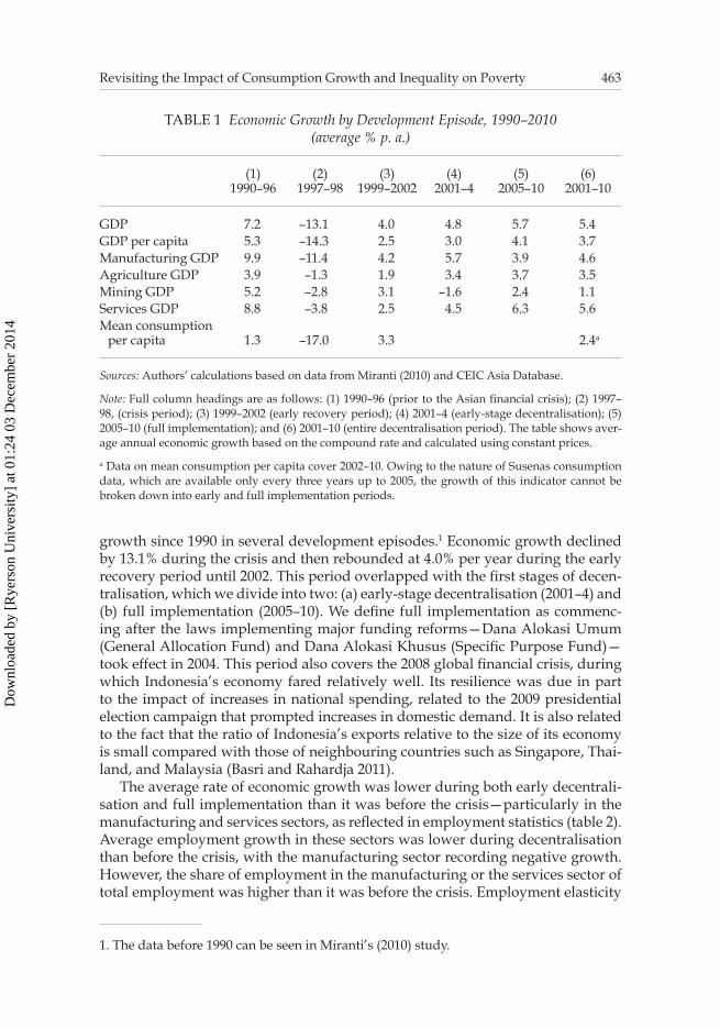
TABLE 1 Economic Growth by Development Episode, 1990–2010 (average % p. a.)

(1) 1990–96

(2) 1997–98

(3) 1999–2002

(4) 2001–4

(5) 2005–10

(6) 2001–10

GDP 7.2 –13.1 4.0 4.8 5.7 5.4GDP per capita 5.3 –14.3 2.5 3.0 4.1 3.7Manufacturing GDP 9.9 –11.4 4.2 5.7 3.9 4.6Agriculture GDP 3.9 –1.3 1.9 3.4 3.7 3.5Mining GDP 5.2 –2.8 3.1 –1.6 2.4 1.1Services GDP 8.8 –3.8 2.5 4.5 6.3 5.6Mean consumption per capita 1.3 –17.0 3.3 2.4a

Sources: Authors’ calculations based on data from Miranti (2010) and CEIC Asia Database.

Note: Full column headings are as follows: (1) 1990–96 (prior to the Asian financial crisis); (2) 1997–98, (crisis period); (3) 1999–2002 (early recovery period); (4) 2001–4 (earlystage decentralisation); (5) 2005–10 (full implementation); and (6) 2001–10 (entire decentralisation period). The table shows aver-age annual economic growth based on the compound rate and calculated using constant prices.

a Data on mean consumption per capita cover 2002–10. Owing to the nature of Susenas consumption data, which are available only every three years up to 2005, the growth of this indicator cannot be broken down into early and full implementation periods.

growth since 1990 in several development episodes.1 Economic growth declined by 13.1% during the crisis and then rebounded at 4.0% per year during the early recovery period until 2002. This period overlapped with the first stages of decen-tralisation, which we divide into two: (a) earlystage decentralisation (2001–4) and (b) full implementation (2005–10). We define full implementation as commenc-ing after the laws implementing major funding reforms—Dana Alokasi Umum (General Allocation Fund) and Dana Alokasi Khusus (Specific Purpose Fund)—took effect in 2004. This period also covers the 2008 global financial crisis, during which Indonesia’s economy fared relatively well. Its resilience was due in part to the impact of increases in national spending, related to the 2009 presidential election campaign that prompted increases in domestic demand. It is also related to the fact that the ratio of Indonesia’s exports relative to the size of its economy is small compared with those of neighbouring countries such as Singapore, Thai-land, and Malaysia (Basri and Rahardja 2011).

The average rate of economic growth was lower during both early decentrali-sation and full implementation than it was before the crisis—particularly in the manufacturing and services sectors, as reflected in employment statistics (table 2). Average employment growth in these sectors was lower during decentralisation than before the crisis, with the manufacturing sector recording negative growth. However, the share of employment in the manufacturing or the services sector of total employment was higher than it was before the crisis. Employment elasticity

1. The data before 1990 can be seen in Miranti’s (2010) study.

Dow

nloa

ded

by [

Rye

rson

Uni

vers

ity]

at 0

1:24

03

Dec

embe

r 20

14


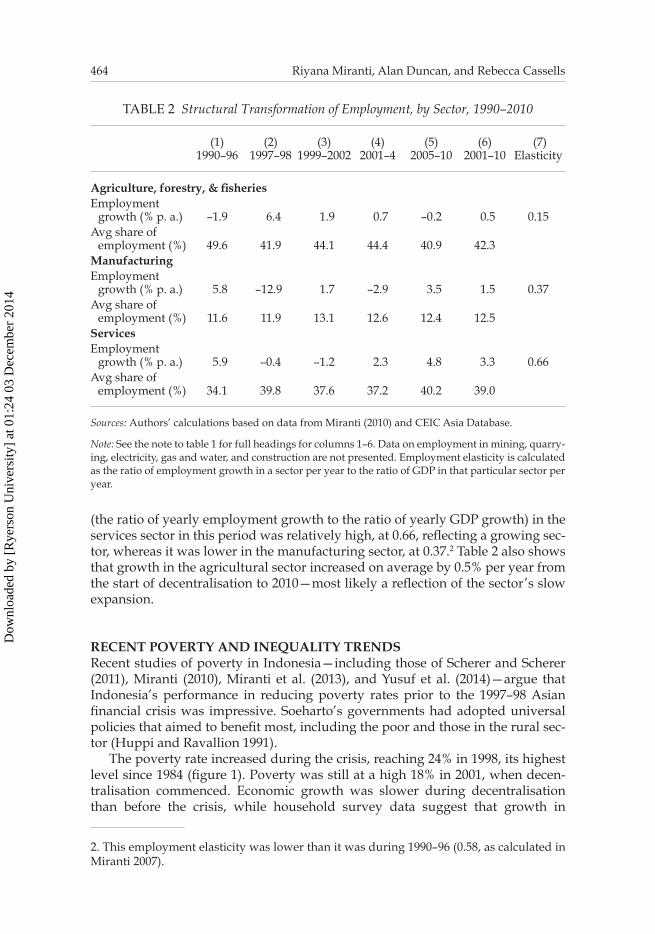
TABLE 2 Structural Transformation of Employment, by Sector, 1990–2010

(1) 1990–96

(2) 1997–98

(3) 1999–2002

(4) 2001–4

(5) 2005–10

(6) 2001–10

(7) Elasticity

Agriculture, forestry, & fisheriesEmployment growth (% p. a.) –1.9 6.4 1.9 0.7 –0.2 0.5 0.15Avg share of employment (%) 49.6 41.9 44.1 44.4 40.9 42.3ManufacturingEmployment growth (% p. a.) 5.8 –12.9 1.7 –2.9 3.5 1.5 0.37Avg share of employment (%) 11.6 11.9 13.1 12.6 12.4 12.5ServicesEmployment growth (% p. a.) 5.9 –0.4 –1.2 2.3 4.8 3.3 0.66Avg share of employment (%) 34.1 39.8 37.6 37.2 40.2 39.0

Sources: Authors’ calculations based on data from Miranti (2010) and CEIC Asia Database.

Note: See the note to table 1 for full headings for columns 1–6. Data on employment in mining, quarry-ing, electricity, gas and water, and construction are not presented. Employment elasticity is calculated as the ratio of employment growth in a sector per year to the ratio of GDP in that particular sector per year.

(the ratio of yearly employment growth to the ratio of yearly GDP growth) in the services sector in this period was relatively high, at 0.66, reflecting a growing sec-tor, whereas it was lower in the manufacturing sector, at 0.37.2 Table 2 also shows that growth in the agricultural sector increased on average by 0.5% per year from the start of decentralisation to 2010—most likely a reflection of the sector’s slow expansion.

RECENT POVERTY AND INEQUALITY TRENDSRecent studies of poverty in Indonesia—including those of Scherer and Scherer (2011), Miranti (2010), Miranti et al. (2013), and Yusuf et al. (2014)—argue that Indonesia’s performance in reducing poverty rates prior to the 1997–98 Asian financial crisis was impressive. Soeharto’s governments had adopted universal policies that aimed to benefit most, including the poor and those in the rural sec-tor (Huppi and Ravallion 1991).

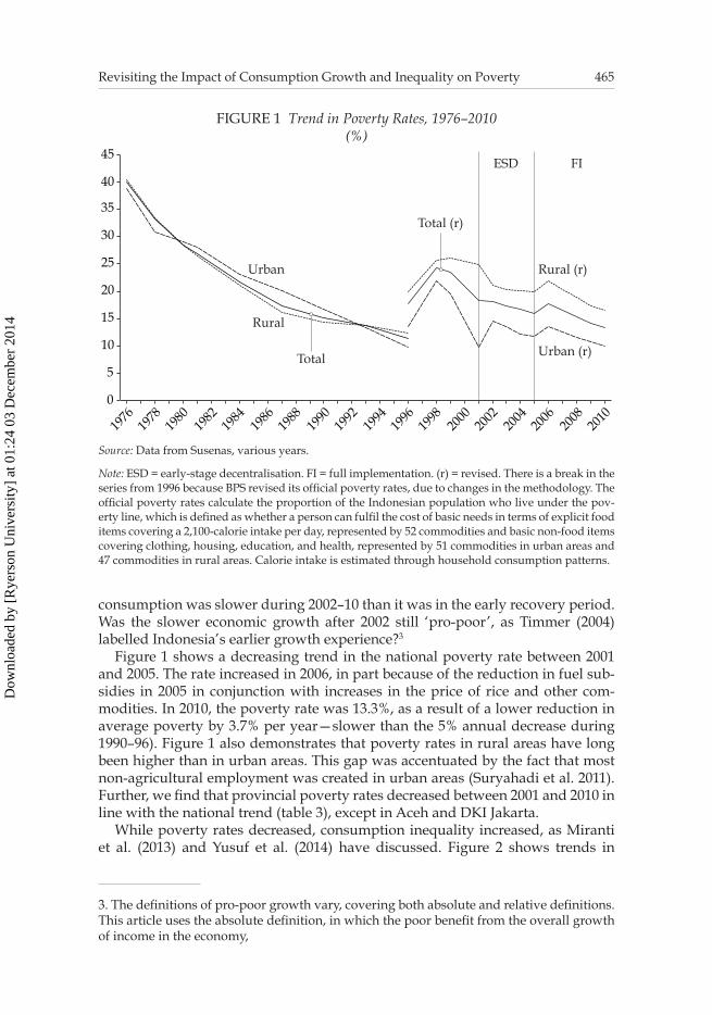
The poverty rate increased during the crisis, reaching 24% in 1998, its highest level since 1984 (figure 1). Poverty was still at a high 18% in 2001, when decen-tralisation commenced. Economic growth was slower during decentralisation than before the crisis, while household survey data suggest that growth in

2. This employment elasticity was lower than it was during 1990–96 (0.58, as calculated in Miranti 2007).

Dow

nloa

ded

by [

Rye

rson

Uni

vers

ity]

at 0

1:24

03

Dec

embe

r 20

14


FIGURE 1 Trend in Poverty Rates, 1976–2010 (%)

1976

1978

1980

1982

1984

1986

1988

1990

1992

1994

1996

1998

2000

2002

2004

2006

2008

2010

0

5

10

15

20

25

30

35

40

45ESD FI

Total

Urban

Rural

Rural (r)

Total (r)

Urban (r)

Source: Data from Susenas, various years.

Note: ESD = earlystage decentralisation. FI = full implementation. (r) = revised. There is a break in the series from 1996 because BPS revised its official poverty rates, due to changes in the methodology. The official poverty rates calculate the proportion of the Indonesian population who live under the pov-erty line, which is defined as whether a person can fulfil the cost of basic needs in terms of explicit food items covering a 2,100calorie intake per day, represented by 52 commodities and basic nonfood items covering clothing, housing, education, and health, represented by 51 commodities in urban areas and 47 commodities in rural areas. Calorie intake is estimated through household consumption patterns.

consumption was slower during 2002–10 than it was in the early recovery period. Was the slower economic growth after 2002 still ‘propoor’, as Timmer (2004) labelled Indonesia’s earlier growth experience?3

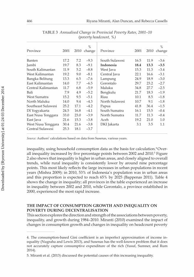
Figure 1 shows a decreasing trend in the national poverty rate between 2001 and 2005. The rate increased in 2006, in part because of the reduction in fuel sub-sidies in 2005 in conjunction with increases in the price of rice and other com-modities. In 2010, the poverty rate was 13.3%, as a result of a lower reduction in average poverty by 3.7% per year—slower than the 5% annual decrease during 1990–96). Figure 1 also demonstrates that poverty rates in rural areas have long been higher than in urban areas. This gap was accentuated by the fact that most nonagricultural employment was created in urban areas (Suryahadi et al. 2011). Further, we find that provincial poverty rates decreased between 2001 and 2010 in line with the national trend (table 3), except in Aceh and DKI Jakarta.

While poverty rates decreased, consumption inequality increased, as Miranti et al. (2013) and Yusuf et al. (2014) have discussed. Figure 2 shows trends in

3. The definitions of propoor growth vary, covering both absolute and relative definitions. This article uses the absolute definition, in which the poor benefit from the overall growth of income in the economy,

Dow

nloa

ded

by [

Rye

rson

Uni

vers

ity]

at 0

1:24

03

Dec

embe

r 20

14


TABLE 3 Annualised Change in Provincial Poverty Rates, 2001–10 (poverty headcount, %)

Province 2001 2010%

change Province 2001 2010%

change

Banten 17.2 7.2 –9.3 South Sulawesi 16.5 11.9 –3.6Jambi 19.7 8.3 –9.1 Indonesia 18.4 13.3 –3.5South Kalimantan 11.9 5.2 –8.8 West Java 15.3 11.3 –3.4West Kalimantan 19.2 9.0 –8.1 Central Java 22.1 16.6 –3.1Bangka Belitung 13.3 6.5 –7.6 Lampung 24.9 18.9 –3.0East Kalimantan 14.0 7.7 –6.5 Gorontalo 29.7 23.2 –2.7Central Kalimantan 11.7 6.8 –5.9 Maluku 34.8 27.7 –2.5Bali 7.9 4.9 –5.2 Bengkulu 21.7 18.3 –1.9West Sumatra 15.2 9.5 –5.1 Riau 10.1 8.5 –1.8North Maluku 14.0 9.4 –4.3 North Sulawesi 10.7 9.1 –1.8Southeast Sulawesi 25.2 17.1 –4.2 Papua 41.8 36.4 –1.5DI Yogyakarta 24.5 16.8 –4.1 South Sumatra 16.1 15.5 –0.4East Nusa Tenggara 33.0 23.0 –3.9 North Sumatra 11.7 11.3 –0.4East Java 21.6 15.3 –3.8 Aceh 19.2 21.0 1.0West Nusa Tenggara 30.4 21.6 –3.8 DKI Jakarta 3.1 3.5 1.1Central Sulawesi 25.3 18.1 –3.7

Source: Authors’ calculations based on data from Susenas, various years.

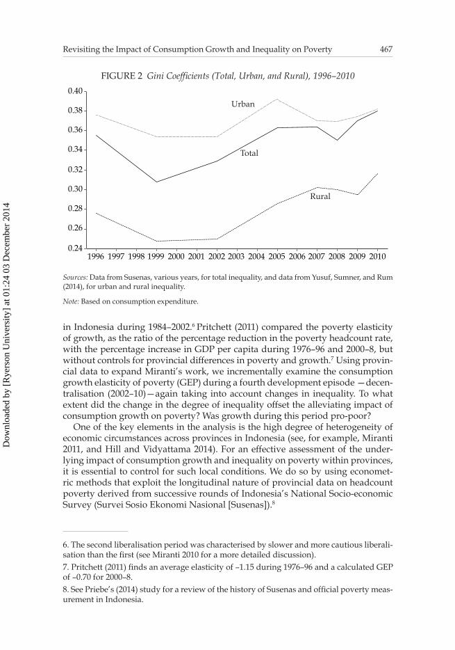
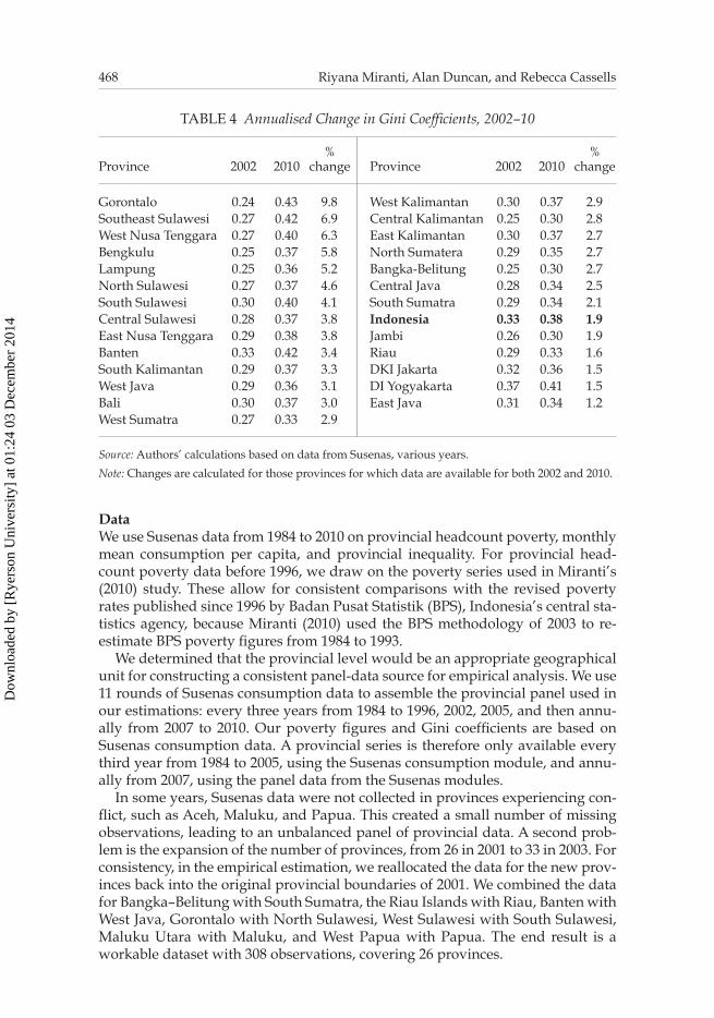
inequality, using household consumption data as the basis for calculation.4 Over-all inequality increased by five percentage points between 2002 and 2010.5 Figure 2 also shows that inequality is higher in urban areas, and closely aligned to overall trends, while rural inequality is consistently lower by around nine percentage points. This most likely reflects the large increases in urban populations in recent years (Mishra 2009): in 2010, 53% of Indonesia’s population was in urban areas and this proportion is expected to reach 65% by 2025 (Bappenas 2011). Table 4 shows the change in inequality; all provinces in the table experienced an increase in inequality between 2002 and 2010, while Gorontalo, a province established in 2000, experienced the most rapid increase.

THE IMPACT OF CONSUMPTION GROWTH AND INEQUALITY ON POVERTY DURING DECENTRALISATION This section explores the direction and strength of the associations between poverty, inequality, and growth during 1984–2010. Miranti (2010) examined the impact of changes in consumption growth and changes in inequality on headcount poverty

4. The consumptionbased Gini coefficient is an imperfect approximation of income in-equality (Nugraha and Lewis 2013), and Susenas has the wellknown problem that it does not accurately capture consumptive expenditure of the rich (Yusuf, Sumner, and Rum 2014).5. Miranti et al. (2013) discussed the potential causes of this increasing inequality.

Dow

nloa

ded

by [

Rye

rson

Uni

vers

ity]

at 0

1:24

03

Dec

embe

r 20

14


FIGURE 2 Gini Coefficients (Total, Urban, and Rural), 1996–2010

Rural

Total

Urban

1996 1997 1998 1999 2000 2001 2002 2003 2004 2005 2006 2007 2008 2009 20100.24

0.26

0.28

0.30

0.32

0.34

0.36

0.38

0.40

Sources: Data from Susenas, various years, for total inequality, and data from Yusuf, Sumner, and Rum (2014), for urban and rural inequality.

Note: Based on consumption expenditure.

in Indonesia during 1984–2002.6 Pritchett (2011) compared the poverty elasticity of growth, as the ratio of the percentage reduction in the poverty headcount rate, with the percentage increase in GDP per capita during 1976–96 and 2000–8, but without controls for provincial differences in poverty and growth.7 Using provin-cial data to expand Miranti’s work, we incrementally examine the consumption growth elasticity of poverty (GEP) during a fourth development episode —decen-tralisation (2002–10)—again taking into account changes in inequality. To what extent did the change in the degree of inequality offset the alleviating impact of consumption growth on poverty? Was growth during this period propoor?

One of the key elements in the analysis is the high degree of heterogeneity of economic circumstances across provinces in Indonesia (see, for example, Miranti 2011, and Hill and Vidyattama 2014). For an effective assessment of the underlying impact of consumption growth and inequality on poverty within provinces, it is essential to control for such local conditions. We do so by using economet-ric methods that exploit the longitudinal nature of provincial data on headcount poverty derived from successive rounds of Indonesia’s National Socioeconomic Survey (Survei Sosio Ekonomi Nasional [Susenas]).8

6. The second liberalisation period was characterised by slower and more cautious liberali-sation than the first (see Miranti 2010 for a more detailed discussion).7. Pritchett (2011) finds an average elasticity of –1.15 during 1976–96 and a calculated GEP of –0.70 for 2000–8. 8. See Priebe’s (2014) study for a review of the history of Susenas and official poverty meas-urement in Indonesia.

Dow

nloa

ded

by [

Rye

rson

Uni

vers

ity]

at 0

1:24

03

Dec

embe

r 20

14


TABLE 4 Annualised Change in Gini Coefficients, 2002–10

Province 2002 2010%

change Province 2002 2010%

change

Gorontalo 0.24 0.43 9.8 West Kalimantan 0.30 0.37 2.9 Southeast Sulawesi 0.27 0.42 6.9 Central Kalimantan 0.25 0.30 2.8 West Nusa Tenggara 0.27 0.40 6.3 East Kalimantan 0.30 0.37 2.7 Bengkulu 0.25 0.37 5.8 North Sumatera 0.29 0.35 2.7 Lampung 0.25 0.36 5.2 BangkaBelitung 0.25 0.30 2.7 North Sulawesi 0.27 0.37 4.6 Central Java 0.28 0.34 2.5 South Sulawesi 0.30 0.40 4.1 South Sumatra 0.29 0.34 2.1 Central Sulawesi 0.28 0.37 3.8 Indonesia 0.33 0.38 1.9 East Nusa Tenggara 0.29 0.38 3.8 Jambi 0.26 0.30 1.9 Banten 0.33 0.42 3.4 Riau 0.29 0.33 1.6 South Kalimantan 0.29 0.37 3.3 DKI Jakarta 0.32 0.36 1.5 West Java 0.29 0.36 3.1 DI Yogyakarta 0.37 0.41 1.5 Bali 0.30 0.37 3.0 East Java 0.31 0.34 1.2 West Sumatra 0.27 0.33 2.9

Source: Authors’ calculations based on data from Susenas, various years.

Note: Changes are calculated for those provinces for which data are available for both 2002 and 2010.

DataWe use Susenas data from 1984 to 2010 on provincial headcount poverty, monthly mean consumption per capita, and provincial inequality. For provincial head-count poverty data before 1996, we draw on the poverty series used in Miranti’s (2010) study. These allow for consistent comparisons with the revised poverty rates published since 1996 by Badan Pusat Statistik (BPS), Indonesia’s central sta-tistics agency, because Miranti (2010) used the BPS methodology of 2003 to reestimate BPS poverty figures from 1984 to 1993.

We determined that the provincial level would be an appropriate geographical unit for constructing a consistent paneldata source for empirical analysis. We use 11 rounds of Susenas consumption data to assemble the provincial panel used in our estimations: every three years from 1984 to 1996, 2002, 2005, and then annu-ally from 2007 to 2010. Our poverty figures and Gini coefficients are based on Susenas consumption data. A provincial series is therefore only available every third year from 1984 to 2005, using the Susenas consumption module, and annu-ally from 2007, using the panel data from the Susenas modules.

In some years, Susenas data were not collected in provinces experiencing con-flict, such as Aceh, Maluku, and Papua. This created a small number of missing observations, leading to an unbalanced panel of provincial data. A second prob-lem is the expansion of the number of provinces, from 26 in 2001 to 33 in 2003. For consistency, in the empirical estimation, we reallocated the data for the new prov-inces back into the original provincial boundaries of 2001. We combined the data for Bangka–Belitung with South Sumatra, the Riau Islands with Riau, Banten with West Java, Gorontalo with North Sulawesi, West Sulawesi with South Sulawesi, Maluku Utara with Maluku, and West Papua with Papua. The end result is a workable dataset with 308 observations, covering 26 provinces.

Dow

nloa

ded

by [

Rye

rson

Uni

vers

ity]

at 0

1:24

03

Dec

embe

r 20

14


We use mean per capita consumption (in expenditure terms) from Susenas as a proxy of household income rather than per capita GDP data from national or regional accounts. This follows previous literature in this field (see Deaton 2001, Ravallion and Chen 1997, Ravallion and Chen 2003, Adams 2004, and Miranti 2010) and is justified for four reasons: (a) there is only a weak correlation between provincial headcount poverty and economic growth in both the national and the regional accounts; (b) it has yet to be determined whether increased average liv-ing standards translated into poverty reduction (a trickledown effect); (c) mean consumption per capita is suggested to reflect the welfare level more accurately than income from the national accounts (Ravallion 1995), because of its effective-ness in capuring the life cycle or permanent income and is therefore suitable for poverty analysis and (d) our regressions require consistent time series that com-plement those used by Miranti (2007, 2010).

Neither mean per capita consumption nor per capita GDP is free from measure-ment errors; both may underestimate or overestimate household income. Bhalla (2002), for example, has argued that using the survey mean as a growth proxy can greatly underestimate the GEP in developing countries. Adams (2004) found the opposite. Ravallion (2001) tried to correct this problem by using the growth rate from the national accounts as an instrumental variable for the growth rate in the survey mean; but the growth rate from the national accounts may not be the best instrument, since it may be correlated with the error terms in the regression. We therefore define growth as the percentage change in mean consumption per capita. (For comparison, appendix table A1 contains the results using regional GDP per capita.)

We use headcount poverty rates, or the proportion of poor people in the pop-ulation, and Gini coefficients to represent, respectively, provincial poverty and inequality (that is, as statistical measures of the dispersion of income distribu-tion). Both are simpler to understand than other poverty and inequality measures, and both variables are officially published by BPS (except for poverty data before 1996) and calculated from Susenas. To allow for comparisons over time, we use mean consumption (expenditure) per capita data in 1984 rupiah, using the ratio of provincial poverty lines to the 1984 provincial poverty line as a deflator.9

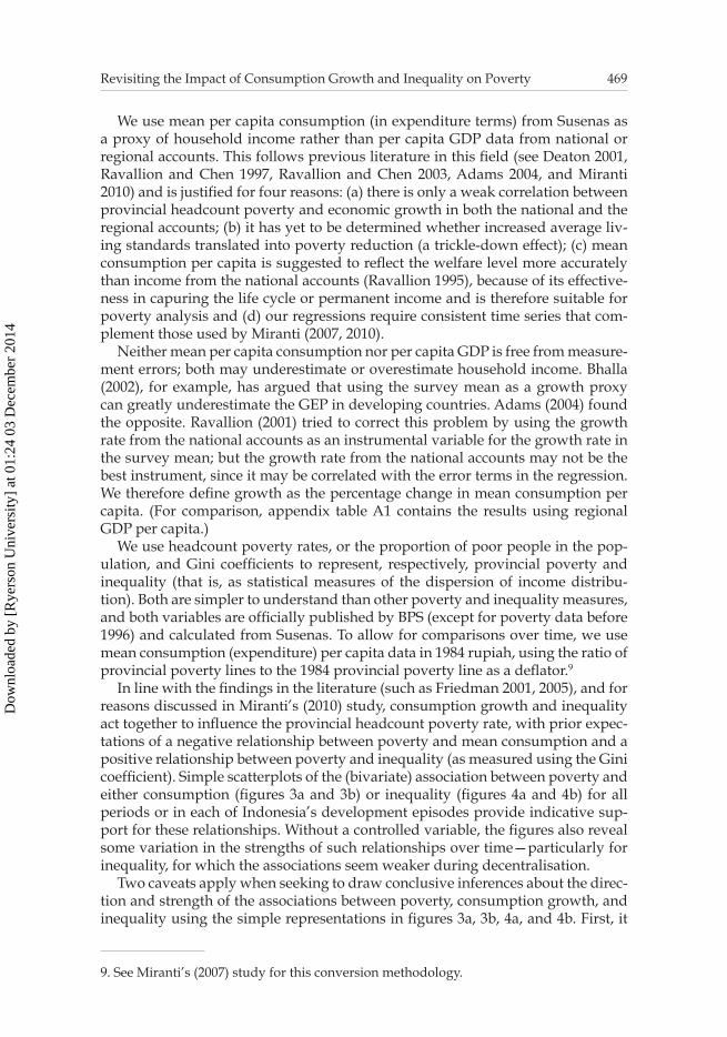
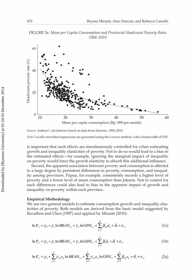
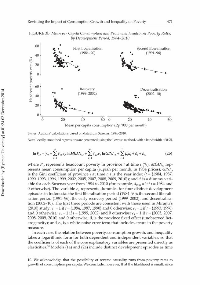
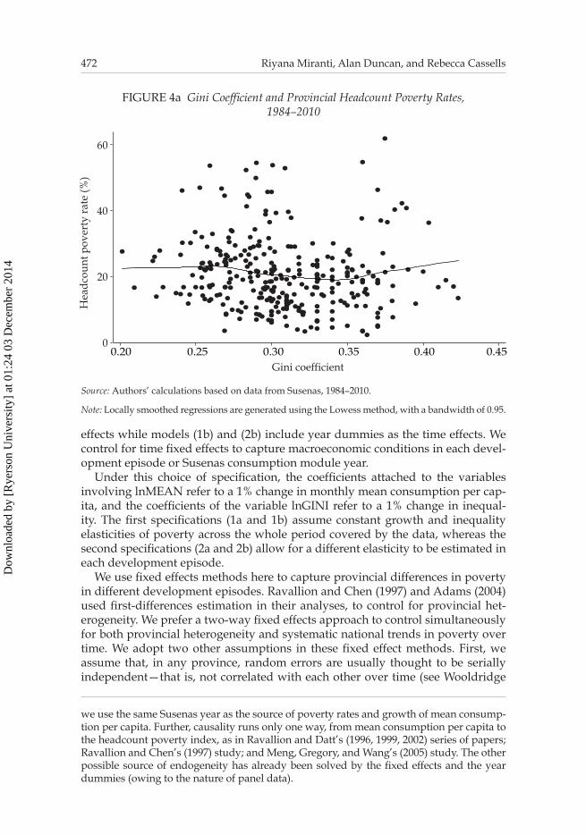
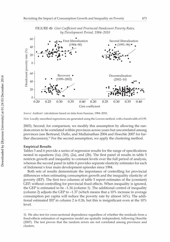
In line with the findings in the literature (such as Friedman 2001, 2005), and for reasons discussed in Miranti’s (2010) study, consumption growth and inequality act together to influence the provincial headcount poverty rate, with prior expec-tations of a negative relationship between poverty and mean consumption and a positive relationship between poverty and inequality (as measured using the Gini coefficient). Simple scatterplots of the (bivariate) association between poverty and either consumption (figures 3a and 3b) or inequality (figures 4a and 4b) for all periods or in each of Indonesia’s development episodes provide indicative sup-port for these relationships. Without a controlled variable, the figures also reveal some variation in the strengths of such relationships over time—particularly for inequality, for which the associations seem weaker during decentralisation.

Two caveats apply when seeking to draw conclusive inferences about the direc-tion and strength of the associations between poverty, consumption growth, and inequality using the simple representations in figures 3a, 3b, 4a, and 4b. First, it

9. See Miranti’s (2007) study for this conversion methodology.

Dow

nloa

ded

by [

Rye

rson

Uni

vers

ity]

at 0

1:24

03

Dec

embe

r 20

14


FIGURE 3a Mean per Capita Consumption and Provincial Headcount Poverty Rates 1984–2010

10 20 30 40 50 600

20

40

60

Mean per capita consumption (Rp ’000 per month)

Hea

dcou

nt p

over

ty r

ate

(%)

Source: Authors’ calculations based on data from Susenas, 1984–2010.

Note: Locally smoothed regressions are generated using the Lowess method, with a bandwidth of 0.95.

is important that such effects are simultaneously controlled for when estimating growth and inequality elasticities of poverty. Not to do so would lead to a bias in the estimated effects—for example, ignoring the marginal impact of inequality on poverty would force the growth elasticity to absorb this additional influence.

Second, the apparent association between poverty and consumption is affected to a large degree by persistent differences in poverty, consumption, and inequal-ity among provinces. Papua, for example, consistently records a higher level of poverty and a lower level of mean consumption than Jakarta. Not to control for such differences could also lead to bias in the apparent impact of growth and inequality on poverty within each province.

Empirical MethodologyWe use two general models to estimate consumption growth and inequality elas-ticities of poverty. Both models are derived from the basic model suggested by Ravallion and Chen (1997) and applied by Miranti (2010):

lnPi,t = γ 0 + γ 1 lnMEANi,t + γ 2 lnGINIi,t + βepdpp=1

P

∑ +δ i + ε i,t (1a)

lnPi,t = γ 0 + γ 1 lnMEANi,t + γ 2 lnGINIi,t + βtdtt=1

T

∑ +δ i + ε i,t

(1b)

lnPi,t = γ 0 + γ 1pp=1

P

∑ ep lnMEANi,t + γ 2 pp=1

P

∑ ep lnGINIi,t + βepepp=1

P

∑ +δ i + ε i,t

(2a)

Dow

nloa

ded

by [

Rye

rson

Uni

vers

ity]

at 0

1:24

03

Dec

embe

r 20

14


FIGURE 3b Mean per Capita Consumption and Provincial Headcount Poverty Rates, by Development Period, 1984–2010

First liberalisation(1984–90)

Second liberalisation(1991–96)

Recovery(1999–2002)

Decentralisation(2002–10)

0

20

40

60

0

20

40

60

20 40 60020 40 600Mean per capita consumption (Rp ’000 per month)

Hea

dcou

nt p

over

ty r

ate

(%)



lnPi,t = γ 0 + γ 1pp=1

P

∑ ep lnMEANi,t + γ 2 pp=1

P

∑ ep lnGINIi,t + βtdtt=1

T

∑ +δ i + ε i,t (2b)

where Pi,t represents headcount poverty in province i at time t (%); MEANi,t rep-resents mean consumption per capita (rupiah per month, in 1984 prices); GINIi,t

is the Gini coefficient of province i at time t; t is the year index (t = {1984, 1987, 1990, 1993, 1996, 1999, 2002, 2005, 2007, 2008, 2009, 2010}); and dt is a dummy vari-able for each Susenas year from 1984 to 2010 (for example, d1984 = 1 if t = 1984 and 0 otherwise). The variable ep represents dummies for four distinct development episodes in Indonesia: the first liberalisation period (1984–90); the second liberali-sation period (1991–96); the early recovery period (1999–2002); and decentralisa-tion (2002–10). The first three periods are consistent with those used in Miranti’s (2010) study: e1 = 1 if t = {1984, 1987, 1990} and 0 otherwise; e2 = 1 if t = {1993, 1996} and 0 otherwise; e3 = 1 if t = {1999, 2002} and 0 otherwise; e4 = 1 if t = {2005, 2007, 2008, 2009, 2010} and 0 otherwise; d i is the province fixed effect (unobserved het-erogeneity); and ei,t is a whitenoise error term that includes errors in the poverty measure.

In each case, the relation between poverty, consumption growth, and inequality takes a logarithmic form for both dependent and independent variables, so that the coefficients of each of the core explanatory variables are presented directly as elasticities.10 Models (1a) and (2a) include distinct development episodes as time

10. We acknowledge that the possibility of reverse causality runs from poverty rates to growth of consumption per capita. We conclude, however, that the likelihood is small, since

Dow

nloa

ded

by [

Rye

rson

Uni

vers

ity]

at 0

1:24

03

Dec

embe

r 20

14


FIGURE 4a Gini Coefficient and Provincial Headcount Poverty Rates, 1984–2010

0.20 0.25 0.30 0.35 0.40 0.450

20

40

60

Gini coefficient

Hea

dcou

nt p

over

ty r

ate

(%)



effects while models (1b) and (2b) include year dummies as the time effects. We control for time fixed effects to capture macroeconomic conditions in each devel-opment episode or Susenas consumption module year.

Under this choice of specification, the coefficients attached to the variables involving lnMEAN refer to a 1% change in monthly mean consumption per cap-ita, and the coefficients of the variable lnGINI refer to a 1% change in inequal-ity. The first specifications (1a and 1b) assume constant growth and inequality elasticities of poverty across the whole period covered by the data, whereas the second specifications (2a and 2b) allow for a different elasticity to be estimated in each development episode.

We use fixed effects methods here to capture provincial differences in poverty in different development episodes. Ravallion and Chen (1997) and Adams (2004) used firstdifferences estimation in their analyses, to control for provincial het-erogeneity. We prefer a twoway fixed effects approach to control simultaneously for both provincial heterogeneity and systematic national trends in poverty over time. We adopt two other assumptions in these fixed effect methods. First, we assume that, in any province, random errors are usually thought to be serially independent—that is, not correlated with each other over time (see Wooldridge

we use the same Susenas year as the source of poverty rates and growth of mean consump-tion per capita. Further, causality runs only one way, from mean consumption per capita to the headcount poverty index, as in Ravallion and Datt’s (1996, 1999, 2002) series of papers; Ravallion and Chen’s (1997) study; and Meng, Gregory, and Wang’s (2005) study. The other possible source of endogeneity has already been solved by the fixed effects and the year dummies (owing to the nature of panel data).

Dow

nloa

ded

by [

Rye

rson

Uni

vers

ity]

at 0

1:24

03

Dec

embe

r 20

14


FIGURE 4b Gini Coefficient and Provincial Headcount Poverty Rates, by Development Period, 1984–2010

0

20

40

60

0

20

40

60

0.25 0.30 0.400.20 0.35

Hea

dcou

nt p

over

ty r

ate

(%)

0.25 0.30 0.400.20 0.35Gini coefficient

First liberalisation(1984–90)

Second liberalisation(1991–96)

Recovery(1999–2002)

Decentralisation(2002–10)



2003). Second, for comparison, we modify this assumption by allowing the ran-dom errors to be correlated within provinces across years but uncorrelated among provinces (see Bertrand, Duflo, and Mullainathan 2004 and Hoechle 2007 for fur-ther discussion).11 For the second assumption, we apply the clustering method.

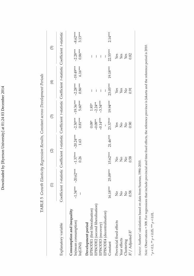
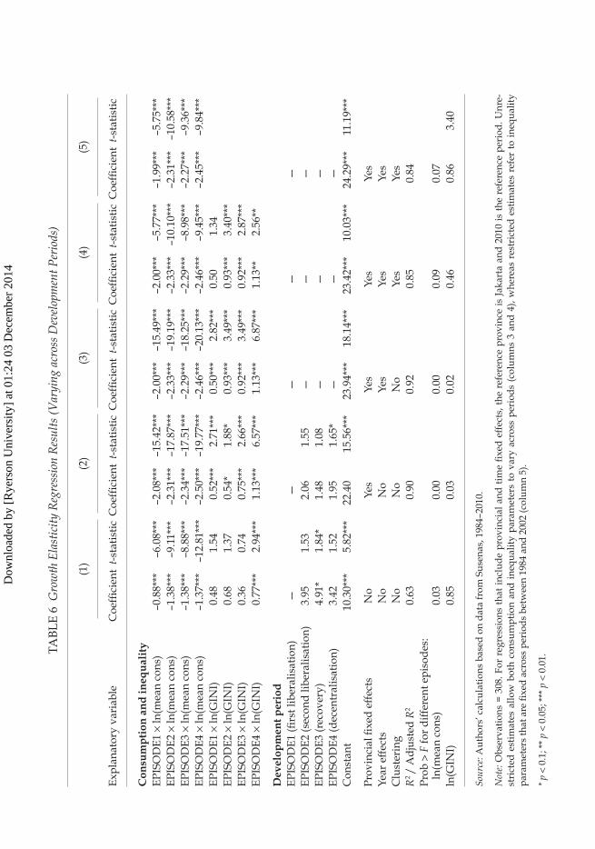
Empirical ResultsTables 5 and 6 provide a series of regression results for the range of specifications nested in equations (1a), (1b), (2a), and (2b). The first panel of results in table 5 restricts growth and inequality to constant levels over the full period of analysis, whereas the second panel in table 6 provides separate elasticity estimates for each of Indonesia’s four main development episodes since 1984.

Both sets of results demonstrate the importance of controlling for provincial differences when estimating consumption growth and the inequality elasticity of poverty (IEP). The first two columns of table 5 report estimates of the (constant) GEP, without controlling for provincial fixed effects. When inequality is ignored, the GEP is estimated to be –1.34 (column 1). The additional control of inequality (column 2) adjusts the GEP to –1.37 (which means that a 10% increase in average consumption per capita will reduce the poverty rate by almost 14%). The addi-tional estimated IEP in column 2 is 0.26, but this is insignificant even at the 10% level.

11. We also test for crosssectional dependence regardless of whether the residuals from a fixedeffects estimation of regression model are spatially independent, following Hoechle (2007). The test proves that the random errors are not correlated among provinces and clusters.

Dow

nloa

ded

by [

Rye

rson

Uni

vers

ity]

at 0

1:24

03

Dec

embe

r 20

14

TABL

E 5

Gro

wth

Ela

stic

ity

Reg

ress

ion

Res

ults

, Con

stan

t acr

oss

Dev

elop

men

t Per

iods

(1)

(2)

(3)

(4)

(5)

Expl

anat

ory

vari

able

Coe

ffici

ent

t-st

atis

ticC

oeffi

cien

tt-

stat

istic

Coe

ffici

ent

t-st

atis

ticC

oeffi

cien

tt-

stat

istic

Coe

ffici

ent

t-st

atis

tic

Con

sum

pti

on a

nd

ineq

ual

ity

ln(m

ean

cons

umpt

ion)

–1.3

4***

–20.

62**

*–1

.37*

**–2

0.24

***

–2.3

0***

–19.

36**

*–2

.28*

**–1

9.49

***

–2.2

8***

–8.6

2***

ln(G

INI)

—0.

261.

630.

81**

*5.

60**

*0.

86**

*6.

16**

*0.

86**

*3.

13**

*

Dev

elop

men

t per

iod

EPIS

OD

E1 (fi

rst l

iber

alis

atio

n)0.

08*

1.85

*—

—EP

ISO

DE2

(sec

ond

liber

alis

atio

n)–0

.08*

*–2

.24*

*—

—EP

ISO

DE3

(rec

over

y)–0

.14*

**–3

.34*

**—

—EP

ISO

DE4

(dec

entr

alis

atio

n)–

——

Con

stan

t16

.18*

**25

.09*

**15

.62*

**21

.46*

**23

.37*

**19

.94*

**23

.05*

**19

.18*

**22

.55*

**2.

14**

*

Prov

inci

al fi

xed

effe

cts

No

No

Yes

Yes

Yes

Year

eff

ects

No

No

No

Yes

Yes

Clu

ster

ing

No

No

No

No

Yes

R2 /

Adj

uste

d R

2 0.

58

0.58

0.

90

0.91

0.

82

Sour

ce: A

utho

rs’ c

alcu

latio

ns b

ased

on

data

from

Sus

enas

, 198

4–20

10.

Not

e: O

bser

vatio

ns =

308

. For

reg

ress

ions

that

incl

ude

prov

inci

al a

nd ti

me

fixed

eff

ects

, the

ref

eren

ce p

rovi

nce

is Ja

kart

a an

d th

e re

fere

nce

peri

od is

201

0.

* p

< 0.

1; *

* p

< 0.

05; *

** p

< 0

.01.

Dow

nloa

ded

by [

Rye

rson

Uni

vers

ity]

at 0

1:24

03

Dec

embe

r 20

14

TABL

E 6

Gro

wth

Ela

stic

ity

Reg

ress

ion

Res

ults

(Var

ying

acr

oss

Dev

elop

men

t Per

iods

)

(1)

(2)

(3)

(4)

(5)

Expl

anat

ory

vari

able

Coe

ffici

ent

t-st

atis

ticC

oeffi

cien

tt-

stat

istic

Coe

ffici

ent

t-st

atis

ticC

oeffi

cien

tt-

stat

istic

Coe

ffici

ent

t-st

atis

tic

Con

sum

pti

on a

nd

ineq

ual

ity

EPIS

OD

E1 ×

ln(m

ean

cons

)–0

.88*

**–6

.08*

**–2

.08*

**–1

5.42

***

–2.0

0***

–15.

49**

*–2

.00*

**–5

.77*

**–1

.99*

**–5

.75*

**EP

ISO

DE2

× ln

(mea

n co

ns)

–1.3

8***

–9.1

1***

–2.3

1***

–17.

87**

*–2

.33*

**–1

9.19

***

–2.3

3***

–10.

10**

*–2

.31*

**–1

0.58

***

EPIS

OD

E3 ×

ln(m

ean

cons

)–1

.38*

**–8

.88*

**–2

.34*

**–1

7.51

***

–2.2

9***

–18.

25**

*–2

.29*

**–8

.98*

**–2

.27*

**–9

.36*

**EP

ISO

DE4

× ln

(mea

n co

ns)

–1.3

7***

–12.

81**

*–2

.50*

**–1

9.77

***

–2.4

6***

–20.

13**

*–2

.46*

**–9

.45*

**–2

.45*

**–9

.84*

**EP

ISO

DE1

× ln

(GIN

I)0.

481.

540.

52**

*2.

71**

*0.

50**

*2.

82**

*0.

501.

34EP

ISO

DE2

× ln

(GIN

I)0.

681.

370.

54*

1.88

*0.

93**

*3.

49**

*0.

93**

*3.

40**

*EP

ISO

DE3

× ln

(GIN

I)0.

360.

740.

75**

*2.

66**

*0.

92**

*3.

49**

*0.

92**

*2.

87**

*EP

ISO

DE4

× ln

(GIN

I)0.

77**

*2.

94**

*1.

13**

*6.

57**

*1.

13**

*6.

87**

*1.

13**

2.56

**

Dev

elop

men

t per

iod

EPIS

OD

E1 (fi

rst l

iber

alis

atio

n)—

——

——

EPIS

OD

E2 (s

econ

d lib

eral

isat

ion)

3.95

1.53

2.06

1.55

——

—EP

ISO

DE3

(rec

over

y)4.

91*

1.84

*1.

481.

08—

——

EPIS

OD

E4 (d

ecen

tral

isat

ion)

3.42

1.52

1.95

1.65

*—

——

Con

stan

t10

.30*

**5.

82**

*22

.40

15.5

6***

23.9

4***

18.1

4***

23.4

2***

10.0

3***

24.2

9***

11.1

9***

Prov

inci

al fi

xed

effe

cts

No

Yes

Yes

Yes

Yes

Year

eff

ects

No

No

Yes

Yes

Yes

Clu

ster

ing

No

No

No

Yes

Yes

R2 /

Adj

uste

d R

2 0.

63

0.90

0.

92

0.85

0.84

Pr

ob >

F fo

r di

ffer

ent e

piso

des:

ln(m

ean

cons

)0.

030.

000.

000.

090.

07ln

(GIN

I)0.

850.

030.

020.

460.

86

3.40

Sour

ce: A

utho

rs’ c

alcu

latio

ns b

ased

on

data

from

Sus

enas

, 198

4–20

10.

Not

e: O

bser

vatio

ns =

308

. For

reg

ress

ions

tha

t in

clud

e pr

ovin

cial

and

tim

e fix

ed e

ffec

ts, t

he r

efer

ence

pro

vinc

e is

Jak

arta

and

201

0 is

the

ref

eren

ce p

erio

d. U

nre-

stri

cted

est

imat

es a

llow

bot

h co

nsum

ptio

n an

d in

equa

lity

para

met

ers

to v

ary

acro

ss p

erio

ds (

colu

mns

3 a

nd 4

), w

here

as r

estr

icte

d es

timat

es r

efer

to

ineq

ualit

y pa

ram

eter

s th

at a

re fi

xed

acro

ss p

erio

ds b

etw

een

1984

and

200

2 (c

olum

n 5)

.

* p

< 0.

1; *

* p

< 0.

05; *

** p

< 0

.01.

Dow

nloa

ded

by [

Rye

rson

Uni

vers

ity]

at 0

1:24

03

Dec

embe

r 20

14


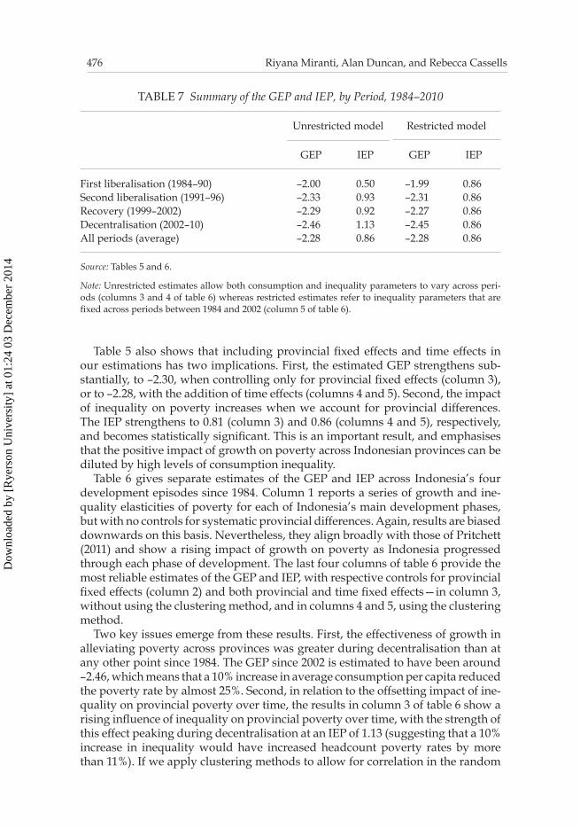
TABLE 7 Summary of the GEP and IEP, by Period, 1984–2010

Unrestricted model Restricted model

GEP IEP GEP IEP

First liberalisation (1984–90) –2.00 0.50 –1.99 0.86Second liberalisation (1991–96) –2.33 0.93 –2.31 0.86Recovery (1999–2002) –2.29 0.92 –2.27 0.86Decentralisation (2002–10) –2.46 1.13 –2.45 0.86All periods (average) –2.28 0.86 –2.28 0.86

Source: Tables 5 and 6.

Note: Unrestricted estimates allow both consumption and inequality parameters to vary across peri-ods (columns 3 and 4 of table 6) whereas restricted estimates refer to inequality parameters that are fixed across periods between 1984 and 2002 (column 5 of table 6).

Table 5 also shows that including provincial fixed effects and time effects in our estimations has two implications. First, the estimated GEP strengthens sub-stantially, to –2.30, when controlling only for provincial fixed effects (column 3), or to –2.28, with the addition of time effects (columns 4 and 5). Second, the impact of inequality on poverty increases when we account for provincial differences. The IEP strengthens to 0.81 (column 3) and 0.86 (columns 4 and 5), respectively, and becomes statistically significant. This is an important result, and emphasises that the positive impact of growth on poverty across Indonesian provinces can be diluted by high levels of consumption inequality.

Table 6 gives separate estimates of the GEP and IEP across Indonesia’s four development episodes since 1984. Column 1 reports a series of growth and ine-quality elasticities of poverty for each of Indonesia’s main development phases, but with no controls for systematic provincial differences. Again, results are biased downwards on this basis. Nevertheless, they align broadly with those of Pritchett (2011) and show a rising impact of growth on poverty as Indonesia progressed through each phase of development. The last four columns of table 6 provide the most reliable estimates of the GEP and IEP, with respective controls for provincial fixed effects (column 2) and both provincial and time fixed effects—in column 3, without using the clustering method, and in columns 4 and 5, using the clustering method.

Two key issues emerge from these results. First, the effectiveness of growth in alleviating poverty across provinces was greater during decentralisation than at any other point since 1984. The GEP since 2002 is estimated to have been around –2.46, which means that a 10% increase in average consumption per capita reduced the poverty rate by almost 25%. Second, in relation to the offsetting impact of ine-quality on provincial poverty over time, the results in column 3 of table 6 show a rising influence of inequality on provincial poverty over time, with the strength of this effect peaking during decentralisation at an IEP of 1.13 (suggesting that a 10% increase in inequality would have increased headcount poverty rates by more than 11%). If we apply clustering methods to allow for correlation in the random

Dow

nloa

ded

by [

Rye

rson

Uni

vers

ity]

at 0

1:24

03

Dec

embe

r 20

14


errors over time and within provinces (column 4 of table 6), the inequality effects become less significant. The final series of estimates (column 5) further restrict the IEP to a constant level over time, returning an estimated (constant) effect of 0.86. The effects of other explanatory factors not separately included in the empirical specifications may be absorbed into year fixed effects and provincial fixed effects. The explanatory variables that have not been included in the estimation include, in particular, relevant government policies or interventions such as various tar-geted poverty alleviation programs.

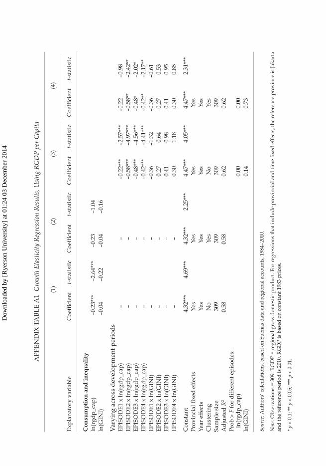
For comparison, we present another measure of income growth: regional gross domestic product (RGDP) per capita (see appendix table A1). The results show that the impact of growth of RGDP on elasticities of poverty is smaller than those that use the consumption data. This is in line with Adams’s (2004) study, which finds a weaker statistical relationship between poverty reduction and the growth of income measured by the national accounts. This may be a limitation of the account data for poverty analysis, since the output produced by a region may not necessarily be associated with the welfare of that particular region (see columns 3 and 4 of appendix table A1). This result supports Miranti’s (2013) study, which examines the determinants of regional poverty in Indonesia during 2006–11 and finds that the GEP during this period using the RGDP per capita as a proxy for income growth is estimated to be low, at –0.28.12

Appendix table A1 also shows that although the GEP was negative and signifi-cant during decentralisation, it was lower than the elasticities during the second liberalisation period and the recovery period. None of those inequality elasticities of poverty is statistically significant.

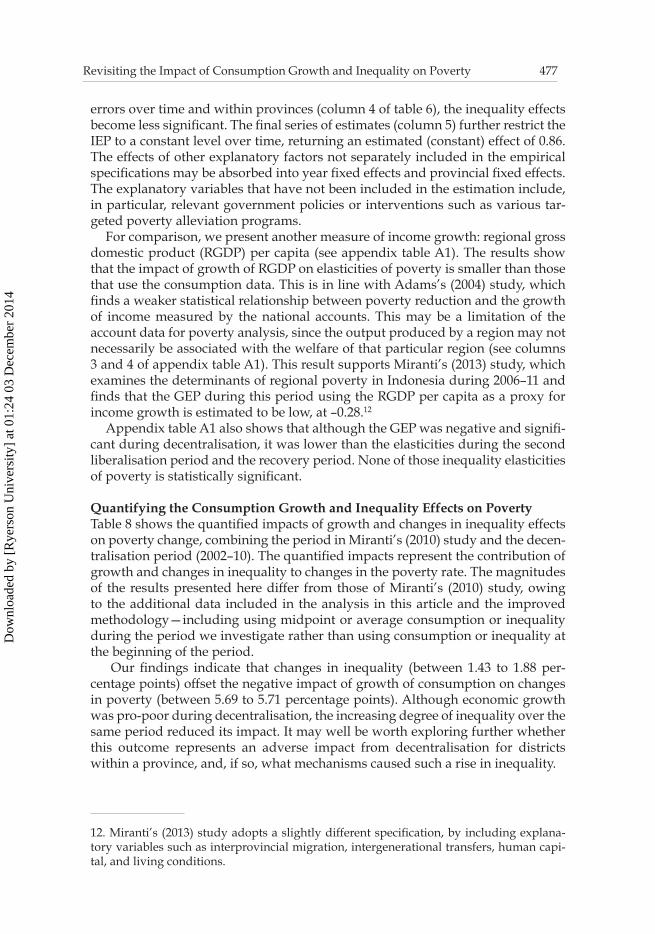
Quantifying the Consumption Growth and Inequality Effects on PovertyTable 8 shows the quantified impacts of growth and changes in inequality effects on poverty change, combining the period in Miranti’s (2010) study and the decen-tralisation period (2002–10). The quantified impacts represent the contribution of growth and changes in inequality to changes in the poverty rate. The magnitudes of the results presented here differ from those of Miranti’s (2010) study, owing to the additional data included in the analysis in this article and the improved methodology—including using midpoint or average consumption or inequality during the period we investigate rather than using consumption or inequality at the beginning of the period.

Our findings indicate that changes in inequality (between 1.43 to 1.88 per-centage points) offset the negative impact of growth of consumption on changes in poverty (between 5.69 to 5.71 percentage points). Although economic growth was propoor during decentralisation, the increasing degree of inequality over the same period reduced its impact. It may well be worth exploring further whether this outcome represents an adverse impact from decentralisation for districts within a province, and, if so, what mechanisms caused such a rise in inequality.

12. Miranti’s (2013) study adopts a slightly different specification, by including explana-tory variables such as interprovincial migration, intergenerational transfers, human capi-tal, and living conditions.

Dow

nloa

ded

by [

Rye

rson

Uni

vers

ity]

at 0

1:24

03

Dec

embe

r 20

14


TABLE 8 Contribution of Consumption Growth and Inequality to Change in Poverty, by Period (percentage points)

Contribution to poverty change

Total poverty changeGrowth

Inequality change

Unrestricted modelFirst liberalisation (1984–90) –3.54 –0.61 –4.15Second liberalisation (1991–96) 0.54 0.79 1.33Recovery (1999–2002) –4.84 0.99 –3.85Decentralisation (2002–10) –5.71 1.88 –3.83All periods (average) –13.55 3.05 –10.50

Restricted modelFirst liberalisation (1984–90) –3.53 –1.05 –4.58Second liberalisation (1991–96) 0.53 0.73 1.26Recovery (1999–2002) –4.80 0.93 –3.87Decentralisation (2002–10) –5.69 1.43 –4.26All periods (average) –13.49 2.04 –11.45

Source: Authors’ calculations.

Note: Unrestricted estimates allow both consumption and inequality parameters to vary across periods (columns 3 and 4 of table 6) whereas restricted estimates refer to inequality parameters that are fixed across periods between 1984 and 2002 (column 5 of table 6).

CONCLUSIONSThis article uses 11 rounds of Susenas consumption modules to calculate the impact of consumption growth and inequality on poverty, focusing on the decen-tralisation period and taking into account unobserved heterogeneity among prov-inces. The results show that the GEP during decentralisation was negative and significant, which means that an increase in average living standards in terms of consumption per capita went hand in hand with poverty reduction. In contrast, the IEP was positive and significant, which suggests that increasing inequality was associated with an increasing poverty rate. From the findings of the unrestricted model, there were more pronounced effects of income inequality on regional pov-erty rates during later development episodes up to the post2002 decentralisation. The propoor impact of economic growth, using mean consumption per capita as a proxy of economic growth during decentralisation (a reduction of around 5.7 percentage points in the headcount poverty rate), was offset to a greater extent by rising income inequality as measured by the Gini coefficient (up from 0.33 in 2002 to 0.38 in 2010). In combination, the stronger negative impact of rising inequality contributed to an increase of between 1.4 to 1.9 percentage points in the headcount poverty rate, offsetting the reduction in the poverty rate by a quarter to onethird.

The impact of different episodes on poverty differs over time; the quantified impact of consumption growth and inequality on poverty was the greatest dur-ing decentralisation. In addition, the results also suggest that changes in inequal-ity offset some of the negative impacts of consumption growth on changes in

Dow

nloa

ded

by [

Rye

rson

Uni

vers

ity]

at 0

1:24

03

Dec

embe

r 20

14


poverty. Although consumption growth was propoor during decentralisation—as in other development episodes (the first and second liberalisation period and the recovery period)—the offsetting effects of changes in inequality hampered the impact of consumption growth during 2002–10.

The fact that increases in inequality countered propoor growth may have some relevant policy implications. Indonesia may need to have more specific policies to combat inequality and poverty rather than just relying on economic growth as a poverty alleviation strategy. Reducing poverty in Indonesia would be more effective under policies that considered local geographic patterns of growth and interprovincial inequality.

REFERENCES Adams, Richard H., Jr. 2004. ‘Economic Growth, Inequality and Poverty: Estimating the

Growth Elasticity of Poverty’. World Development 32 (11): 1989–2014.Basri, Muhammad Chatib, and Sjamsu Rahardja. 2011. ‘Mild Crisis, Half Hearted Fiscal

Stimulus: Indonesia during the GFC’. In Assessment on the Impact of Stimulus, Fiscal Transparency and Fiscal Risk, ERIA Research Project Report 2010-1, edited by Takatoshi Ito and Friska Parulian, 169–211. Jakarta: Economic Research Institute for ASEAN and East Asia.

Bertrand, Marianne, Esther Duflo, and Sendhil Mullainathan. 2004. ‘How Much Should We Trust DifferencesinDifferences Estimates?’. The Quarterly Journal of Economics 119 (1): 249–75.

Bhalla, Surjit S. 2002. Imagine There’s No Country: Poverty, Inequality, and Growth in the Era of Globalization. Washington, DC: Institute for International Economics.

Brodjonegoro, Bambang. 2009. ‘Fiscal Decentralization and Its Impact on Regional Eco-nomic Development and Fiscal Sustainability’. In Decentralization and Regional Auton-omy in Indonesia: Implementation and Challenges, edited by Coen J. G. Holtzappel and Martin Ramstedt, 196–221. Singapore: Institute of Southeast Asian Studies.

Deaton, Angus. 2001. ‘Counting the World’s Poor: Problems and Possible Solutions’. The World Bank Research Observer 16 (2): 125–48.

Friedman, Jed. 2001. ‘Measuring Poverty Change in Indonesia, 1984–1996: How Respon-sive is Poverty to Growth?’. In ‘Essays on Development and Transition’, PhD diss., The University of Michigan.

———. 2005, ‘How Responsive is Poverty to Growth? A Regional Analysis of Poverty, Ine-quality and Growth in Indonesia, 1984–99’. In Spatial Inequality and Development, edited by Ravi Kanbur and Anthony. J. Venables, 163–208. New York: Oxford University Press.

Hartono, Djoni, and Tony Irawan. 2008. ‘Decentralization Policy and Equality: A Theil Analysis of Indonesian Income Inequality’. Working Paper in Economics and Devel-opment Studies 200810, Department of Economics, Padjadjaran University, Bandung.

Hill, Hal. 2007. ‘The Indonesian Economy: Growth, Crisis and Recovery’. The Singapore Economic Review 52 (2): 137–66.

Hill, Hal and Yogi Vidyattama. 2014. ‘Hares and Tortoises: Regional Development Dynam-ics in Indonesia’. In Regional Dynamics in a Decentralized Indonesia, edited by Hal Hill, 68–97. Singapore: Institute of Southeast Asian Studies.

Hoechle, Daniel. 2007. ‘Robust Standard Errors for Panel Regressions with CrossSectional Dependence’. Stata Journal 7 (3): 281–312.

Hofman, Bert, and Kai Kaiser. 2002. ‘The Making of the Big Bang and Its Aftermath: A Political Economy Perspective’. Paper presented at ‘Can Decentralization Help Rebuild Indonesia?’, Georgia State University, Atlanta, GA, 1–3 May.

Dow

nloa

ded

by [

Rye

rson

Uni

vers

ity]

at 0

1:24

03

Dec

embe

r 20

14


Holtzappel, Coen J. G. 2009. ‘Introduction: The Regional Governance Reform in Indonesia, 1999–2004’. In Decentralization and Regional Autonomy in Indonesia: Implementation and Challenges, edited by Coen. J. G. Holtzappel and Martin Ramstedt, 1–56. Singapore: Institute of Southeast Asian Studies.

Huppi, Monika, and Martin Ravallion. 1991. ‘The Sectoral Structure of Poverty during an Adjustment Period: Evidence for Indonesia in the Mid1980s’. World Development 19 (12): 1653–78.

Mahi, B. Raksaka. 2010. ‘Intergovernmental Relations and Decentralization in Indonesia: New Arrangements and Their Impacts on Local Welfare’. Economics and Finance in Indo-nesia 58 (2): 149–72.

Meng, Xin, Robert Gregory, and Youjuan Wang. 2005. ‘Poverty, Inequality, and Growth in Urban China, 1986–2000’. Journal of Comparative Economics 33 (4): 710–29.

Ministry of National Development Planning / National Development Planning Agency. 2011. Masterplan: Acceleration and Expansion of Indonesia Economic Development 2011–2025. Jakarta: Bappenas.

Miranti, Riyana. 2007. ‘The Determinants of Regional Poverty in Indonesia: 1984–2002’. PhD diss., The Australian National University.

———. 2010. ‘Poverty in Indonesia 1984–2002: The Impact of Growth and Changes in Ine-quality’. Bulletin of Indonesian Economic Studies 46 (1): 79–97.

———. 2011. ‘Regional Patterns of Poverty in Indonesia: Why Do Some Provinces Perform Better than Others?’. In Employment, Living Standards and Poverty in Contemporary Indo-nesia, edited by Chris Manning and Sudarno Sumarto. Singapore: Institute of Southeast Asian Studies.

———. 2013. Provincial Poverty Rates in Indonesia, 2006–2011. Report prepared for the National Team for the Acceleration of Poverty Reduction. Jakarta: Support for Eco-nomic Analysis Development in Indonesia.

Miranti, Riyana, Yogi Vidyattama, Erick Hansnata, Rebecca Cassells, and Alan Duncan. 2013. ’Trends in Poverty and Inequality in Decentralising Indonesia’. OECD Social, Employment and Migration Working Paper 148, OECD Publishing, Paris.

Mishra, Satish Chandra. 2009. Economic Inequality in Indonesia: Trends, Causes, and Policy Response. Colombo: Strategic Asia.

Nugraha, Kunta, and Phil Lewis. 2013. ‘Towards a Better Measure of Income Inequality inIndonesia’. Bulletin of Indonesian Economic Studies 49 (1): 103–12.Priebe, Jan. 2014. ‘Official Poverty Measurement in Indonesia since 1984: A Methodological

Review’. Bulletin of Indonesian Economic Studies 50 (2): 185–205.Pritchett, Lant. 2011. ‘How Good Are Good Transitions for Growth and Poverty? Indonesia

since Suharto, for Instance?’. In Employment, Living Standards and Poverty in Contempo-rary Indonesia, edited by Chris Manning and Sudarno Sumarto, 23–46. Singapore: Insti-tute of Southeast Asian Studies.

Ravallion, Martin. 1995. ‘Growth and Poverty: Evidence for Developing Countries in the 1980s’. Economic Letters 48 (3–4): 411–17.

———. 2001. ‘Growth, Inequality and Poverty: Looking beyond Averages’. World Devel-opment 29 (11): 1803–15.

Ravallion, Martin, and Benu Bidani. 1994. ‘How Robust Is a Poverty Profile?’. The World Bank Economic Review 8 (1): 75–102.

Ravallion, Martin, and Shaohua Chen. 1997. ‘What Can New Survey Data Tell Us about Recent Changes in Distribution and Poverty ?’. The World Bank Economic Review 11 (2): 357–82.

———. 2003. ‘Measuring ProPoor Growth?’. Economic Letters 78 (1): 93–99.Ravallion, Martin, and Gaurav Datt. 1996. ‘How Important to India’s Poor Is the Sectoral

Composition of Economic Growth?’. The World Bank Economic Review 10 (1): 1–25.

Dow

nloa

ded

by [

Rye

rson

Uni

vers

ity]

at 0

1:24

03

Dec

embe

r 20

14


———. 1999. ‘When Is Growth ProPoor? Evidence from the Diverse Experience of India’s States’. Policy Research Working Paper 2263, World Bank, Washington, DC.

———. 2002. ‘Why Has Economic Growth Been More Propoor in Some States of India than Others?’. Journal of Development Economics 68 (2): 381–400.

Scherer, S. and Scherer, P. 2011. Trends in Inequality and Poverty in Indonesia since the 1990s. Paris: OECD.

Sumarto, Sudarno, Asep Suryahadi, and Alex Arifianto. 2004. ‘Governance and Poverty Reduction: Evidence from Newly Decentralized Indonesia’. SMERU Working Paper, SMERU Research Institute, Jakarta.

Suryahadi, Asep, Umbu Reku Raya, Deswanto Marbun, and Athia Yumma. 2011. ‘Accel-erating Poverty and Vulnerability Reduction: Trends, Opportunities and Constraints’. In Employment, Living Standards and Poverty in Contemporary Indonesia, edited by Chris Manning and Sudarno Sumarto, 68–89. Singapore: Institute of Southeast Asian Studies.

Temple, Jonathan. 2003. ‘Growing into Trouble: Indonesia after 1966’. In In Search of Pros-perity: Analytic Narratives on Economic Growth, edited by Dani Rodrik, 152–83. Princeton, NJ: Princeton University Press.

Thornton, John. 2007. ‘Fiscal Decentralisation and Economic Growth Reconsidered’. Jour-nal of Urban Economics 61 (1): 64–70.

Timmer, C.Peter. 2004. ‘The Road to Propoor Growth: The Indonesian Experience in Regional Perspective’. Bulletin of Indonesian Economic Studies 40 (2): 177–207.

Wooldridge, Jeffrey M. 2003. Introductory Econometrics. 2nd ed. Cincinnati, OH: SouthWestern College Publishing.

Yusuf, Arief Anshory, Andy Sumner, and Irlan Adiyatma Rum. 2014. ‘Twenty Years of Expenditure Inequality in Indonesia, 1993–2013’. Bulletin of Indonesian Economic Studies 50 (2): 243–54.

Dow

nloa

ded

by [

Rye

rson

Uni

vers

ity]

at 0

1:24

03

Dec

embe

r 20

14

APP

END

IX T

ABL

E A

1 G

row

th E

last

icit

y R

egre

ssio

n R

esul

ts, U

sing

RG

DP

per

Cap

ita

Expl

anat

ory

vari

able

(1)

(2)

(3)

(4)

Coe

ffici

ent

t-st

atis

ticC

oeffi

cien

tt-

stat

istic

Coe

ffici

ent

t-st

atis

ticC

oeffi

cien

tt-

stat

istic

Con

sum

pti

on a

nd

ineq

ual

ity

ln(r

gdp_

cap)

–0.2

3***

–2.6

4***

–0.2

3–1

.04

ln(G

INI)

–0.0

4–0

.22

–0.0

4–0

.16

Var

ying

acr

oss

deve

lopm

ent p

erio

dsEP

ISO

DE1

x ln

(rgd

p_ca

p)–

––0

.22*

**–2

.57*

**–0

.22

–0.9

8EP

ISO

DE2

x ln

(rgd

p_ca

p)–

––0

.58*

**–4

.97*

**–0

.58*

*–2

.42*

*EP

ISO

DE3

x ln

(rgd

p_ca

p)–

––0

.48*

**–4

.56*

**–0

.48*

–2.0

2*EP

ISO

DE4

x ln

(rgd

p_ca

p)–

––0

.42*

**–4

.41*

**–0

.42*

*–2

.17*

*EP

ISO

DE1

x ln

(GIN

I)–

––0

.36

–1.3

2–0

.36

–0.6

1EP

ISO

DE2

x ln

(GIN

I)–

–0.

27 0

.64

0.27

0.53

EPIS

OD

E3 x

ln(G

INI)

––

0.41

0.98

0.41

0.95

EPIS

OD

E4 x

ln(G

INI)

––

0.30

1.18

0.30

0.85

Con

stan

t4.

32**

*4.

69**

*4.

32**

*2.

25**

*4.

47**

*4.

05**

*4.

47**

*2.

31**

*Pr

ovin

cial

fixe

d ef

fect

sYe

sYe

sYe

sYe

sYe

ar e

ffec

tsYe

sYe

sYe

sYe

sC

lust

erin

gN

oYe

sN

oYe

sSa

mpl

e si

ze30

930

930

930

9A

djus

ted

R2

0.58

0.

58

0.62

0.62

Prob

> F

for

diff

eren

t epi

sode

s:

ln

(rgd

p_ca

p)0.

000.

00ln

(GIN

I)0.

140.

73

Sour

ce: A

utho

rs’ c

alcu

latio

ns, b

ased

on

Suen

as d

ata

and

regi

onal

acc

ount

s, 1

984–

2010

.

Not

e: O

bser

vatio

ns =

309

. RG

DP

= re

gion

al g

ross

dom

estic

pro

duct

. For

reg

ress

ions

that

incl

ude

prov

inci

al a

nd ti

me

fixed

eff

ects

, the

ref

eren

ce p

rovi

nce

is Ja

kart

a an

d th

e re

fere

nce

peri

od is

201

0. R

GD

P is

bas

ed o

n co

nsta

nt 1

983

pric

es.

* p

< 0.

1; *

* p

< 0.

05; *

** p

< 0

.01.

Dow

nloa

ded

by [

Rye

rson

Uni

vers

ity]

at 0

1:24

03

Dec

embe

r 20

14

recent development

Documents

authors oecd

curtin universitythis

impact of consumption

poverty inindonesia

decentralising indonesia

articletaylor francis

impactof consumption

consumption growth elastici