real-time water vapor maps from a gps surface network...

Real-Time Water Vapor Maps from a GPS Surface Network: Construction,Validation, and Applications

SIEBREN DE HAAN AND IWAN HOLLEMAN

Royal Netherlands Meteorological Institute, De Bilt, Netherlands

ALBERT A. M. HOLTSLAG

Wageningen University, Wageningen, Netherlands

(Manuscript received 29 April 2008, in final form 1 December 2008)

ABSTRACT

In this paper the construction of real-time integrated water vapor (IWV) maps from a surface network of

global positioning system (GPS) receivers is presented. The IWV maps are constructed using a two-

dimensional variational technique with a persistence background that is 15 min old. The background error

covariances are determined using a novel two-step method, which is based on the Hollingsworth–Lonnberg

method. The quality of these maps is assessed by comparison with radiosonde observations and IWV maps

from a numerical weather prediction (NWP) model. The analyzed GPS IWV maps have no bias against

radiosonde observations and a small bias against NWP analysis and forecasts up to 9 h. The standard

deviation with radiosonde observations is around 2 kg m22, and the standard deviation with NWP increases

with increasing forecast length (from 2 kg m22 for the NWP analysis to 4 kg m22 for a forecast length of 48 h).

To illustrate the additional value of these real-time products for nowcasting, three thunderstorm cases are

discussed. The constructed GPS IWV maps are combined with data from the weather radar, a lightning

detection network, and surface wind observations. All cases show that the location of developing thunder-

storms can be identified 2 h prior to initiation in the convergence of moist air.

1. Introduction

At present, radiosonde observations are the most

important operational source for upper-air water vapor

data. These observations are expensive and thus are

sparse in time and space. Global positioning system

(GPS) zenith total delay (ZTD) observations contain

integrated water vapor path information, which can be

used in numerical weather prediction (NWP) models

and for nowcasting severe weather. Assimilation of GPS

observations has a positive impact on the quality of an

NWP model (Macpherson et al. 2007; Poli et al. 2007;

Smith et al. 2007). These high-temporal-resolution wa-

ter vapor measurements are likely to also have a large

impact on forecasting (rapidly) developing systems

(Mazany et al. 2002; de Haan et al. 2002, 2004; de Haan

2006). Note that the method presented by Mazany et al.

(2002) has a lead time of around 12 h.

The current measurements of atmospheric water vapor

by the radiosonde network do not possess the temporal

or the spatial resolution to provide adequate informa-

tion about atmospheric scales that are smaller than

synoptic scales. GPS radio occultation observations con-

tain information on upper-air humidity; however, these

observations are, in fact, combined temperature and

humidity measurements, and the two can only be sep-

arated with additional information (e.g., temperature

profile). Imagery from geostationary satellites provides

more frequent monitoring of the atmospheric water

vapor, but the use of these observations in NWP is

complicated because of problems with height assign-

ment of the observed structures and because of cloud

contamination. These observations are very well suited

for use in nowcasting. Because of use of passive sensors,

however, lower-stratospheric water vapor information

is confounded by overlying clouds or water vapor and is

therefore only valid in cloud-free situations. Humidity

Corresponding author address: Siebren de Haan, Royal Netherlands

Meteorological Institute, P.O. Box 201, 3730 AE De Bilt, Netherlands.

E-mail: [email protected]

1302 J O U R N A L O F A P P L I E D M E T E O R O L O G Y A N D C L I M A T O L O G Y VOLUME 48

DOI: 10.1175/2008JAMC2024.1

� 2009 American Meteorological Society

observations obtained from infrared and microwave

sounders from polar-orbiting satellites suffer from the

same problem. On the other hand, GPS can observe

integrated water vapor (IWV) almost continuously, in-

dependent of clouds and rain.

In this paper a method of constructing GPS IWV

maps from GPS observations is presented. These maps

are validated with radiosonde observations, NWP-

derived integrated water vapor, and GPS IWV estimated

using a different processing network. Assimilation in

NWP is, of course, another way of presenting the data to

the forecasters. However, numerical weather model

data generally have lead times of several hours. In this

paper, we show that the real-time analysis of GPS ob-

servations can be used to bridge this gap. By discussing

three cases, the application for nowcasting of thunder-

storms is illustrated. First, a description of the data

used is given. Next, the method of constructing two-

dimensional IWV maps based on variational techniques

is introduced. This is followed by a validation of the

constructed IWV maps. Then, three cases of thunder-

storm events in the Netherlands are presented.

2. Observations and infrastructure

A GPS receiver measures the delay of the GPS signal

for every GPS satellite in view. By processing all ob-

served slant delays within a certain time window, errors

and unknowns, such as satellite and receiver clock er-

rors, can be estimated. An estimate of the ZTD, which is

the slant delay mapped to the zenith, is determined for

each GPS receiver in the network. The hydrostatic part

of the ZTD, called the zenith hydrostatic delay (ZHD),

which is the vertical integral of dry air density, can be

estimated using the surface pressure (Saastamoinen

1972). The residual part of ZTD is associated with the

vertically integrated column of water vapor overlying

the GPS receiver; that is,

IWV 5 k�1(ZTD� ZHD), (1)

where k depends on the weighted mean temperature of

the atmosphere, which in turn can be approximated by a

linear function of the surface temperature (Davis et al.

1985; Bevis et al. 1994; Baltink et al. 2002).

General-application GPS receivers, such as those for

time synchronization and car navigation, use (inexpen-

sive) single-frequency receivers. The network of GPS

double-frequency receivers used here was initially con-

structed for operational geodetic applications (land sur-

veying; leveling); the network is presented in Fig. 1

(denoted by the black dots). Using two frequencies, the

path delay due to the ionosphere can be eliminated.

Data from this network are processed by the Royal

Netherlands Meteorological Institute (KNMI) every

15 min; the observations are available approximately

5 min after observation time.

In this study, data from a different network are used

in addition to the GPS data from the real-time network

GPS. The additionally used estimates are processed

on a routine basis by the Geodetic Observatory Pecny

(GOP), in the Czech Republic, within the framework of

the Network of European National Meteorological

Services (EUMETNET) GPS Vapor Programme

(E-GVAP). GOP estimates the atmospheric delay two

times per hour; at the start and at the end of each

window of 1 h. The network does not overlap with the

real-time sites and thus samples different parts of the

atmosphere and uses different GPS receivers (denoted

by the stars and squares in Fig. 1). Both processing

schemes use double differencing to eliminate clock er-

rors. Some details of the processing options of the two

schemes are shown in Table 1.

a. Radiosonde

The current system used is a Vaisala, Inc., RS92 ra-

diosonde. This radiosonde has measurement uncer-

tainties (based on experiments) of 0.18C for tempera-

ture, 0.2 hPa for pressure, and 2% for relative humidity

(Vaisala 2006) and is launched from De Bilt, in the

Netherlands, at 0000 and 1200 UTC. De Bilt is denoted

by the large cross in Fig. 1. Besides measurements of

temperature and humidity, information on the wind

speed and direction is inferred from the change in po-

sition of the balloon during its ascent. The current sys-

tem uses a GPS receiver to track the balloon.

b. Weather radar

A weather radar employs scattering of radio-frequency

waves (5.6 GHz/5 cm for C band) to measure precipita-

tion and other particles in the atmosphere [see Doviak

and Zrni�c (1993) for more details]. The intensity of the

atmospheric echoes is converted to the so-called radar

reflectivity Z using the equations for Rayleigh scatter-

ing. The Rayleigh equations are valid when the wave-

length of the radar is much larger than the diameter of

the scatterers (maximum 6 mm for rain). In that case,

the radar reflectivity depends strongly (to the sixth power)

on the diameter of the rain droplets. The radar reflectivity

is a good measure of the strength of the convection

(updrafts) and the amount of condensed moisture in the

atmosphere.

KNMI operates two identical C-band Doppler weather

radars made by SELEX Sistemi Integrati (SELEX

SI). The radar in De Bilt is located at 52.108N, 5.188E.

The radar in Den Helder is located at 52.968N, 4.798E.

JULY 2009 D E H A A N E T A L . 1303

The locations of the weather radars are designated in

Fig. 1 by the open circles. The weather radars have re-

cently been upgraded with digital receivers and a cen-

tralized product generation. Precipitation and wind are

observed with a 14-level elevation scan (between 0.38

and 258) that is repeated every 5 min.

From the three-dimensional scans, pseudo CAPPI

images, that is, horizontal cross sections of radar reflec-

tivity at constant altitude, are produced with a target

height of 800 m above antenna level and a horizontal

resolution of 2.4 km. Radar reflectivity values are con-

verted to rainfall intensities R using a Z–R relationship

(Marshall and Palmer 1948):

Z 5 200R1.6, (2)

with the radar reflectivity Z in millimeters raised to

the sixth power per meter cubed and rainfall rate R

in millimeters per hour. More details on the KNMI

weather radar network can be found in Holleman (2005,

2007).

c. Lightning detection network

KNMI maintains a Surveillance et Alerte Foudre

par Interferometrie Radioelectrique (SAFIR) Lightning

Detection System for monitoring (severe) convection

and for feeding a climatological database. The lightning

detection system consists of four detection stations lo-

cated in the Netherlands and a central processing unit

located at KNMI in De Bilt. In addition to the four

Dutch stations, raw data from three Belgian stations

operated by the Royal Meteorological Institute of

Belgium are processed in real time as well. The loca-

tions of the seven detection stations are shown in Fig. 1

(gray diamonds).

Each lightning detection station consists of three ba-

sic components: a VHF antenna array, a low-frequency

FIG. 1. Location of GPS sites, SAFIR antennas, two weather radars, and the radiosonde

launch site. The crosses denote the HIRLAM grid points. Statistics against HIRLAM are

derived within the validation area (large area), and the dashed area around the radiosonde

launch site at De Bilt is used in section 4a.

TABLE 1. GPS processing options for GOP and KNMI. Both

processing schemes use Bernese 5.2 software. Note that the ob-

servations window of KNMI is not constant over an hour. The start

time of the window is kept constant for an hour; the end time

changes every 15 min.

GOP KNMI

No. of sites 51 28

ZTD estimates Hourly Every 15 min

Min/max baseline (km) 23/3723 25/1653

Min elev cutoff angle (8) 10 10

Obs interval (s) 30 180

Obs window length (h) 12 11.25–12

Mapping function Hydrostatic Niell Hydrostatic Niell

Ocean tide loading Scherneck (1991) Ray (1999)


(LF) sensor, and a single-frequency GPS receiver. The

VHF antenna array consists of five dipole antennas

mounted in a circle and is used for the azimuth deter-

mination of discharges based on interferometry. The

capacitive LF antenna is used for lightning discrimina-

tion, that is, cloud-to-ground (CG) or cloud-to-cloud

discharge, and for time-of-arrival localization of CG

discharges. The GPS receiver provides accurate time

stamps for the observed discharges. The observed light-

ning events are localized by the central processing unit,

and they are distributed in real time to the users.

The localization accuracy of the SAFIR network over

the Netherlands is around 2 km. The false-alarm rate of

the SAFIR network has been assessed using an overlay

with weather radar imagery and is less than 1%. The

detection efficiency for lightning events of the network

is unknown and is currently under investigation. More

details on the technical layout of the SAFIR network

and its performance can be found in Beekhuis and

Holleman (2004) and Holleman et al. (2006).

d. Numerical weather model data

At KNMI, a High-Resolution Limited Area Model

(HIRLAM; Unden et al. 2002) is run operationally. This

NWP model is started every 6 h and has a forecast

length of 48 h. For the period under consideration, the

model had a resolution of 22 km and 40 vertical levels.

Synoptic observations, such as wind, temperature, and

humidity from radiosondes and surface wind and tem-

perature observations, are used to analyze the initial

state of the atmosphere; note that no GPS data were

assimilated. The previous 6-h forecast is used as back-

ground information and, because the model is a limited-

area model, the forecast at the boundaries of the region

is retrieved from the European Centre for Medium-

Range Weather Forecasts forecast fields.

3. Construction of integrated water vapor fields

An objective analysis of total water vapor columns

can be constructed in various ways. The simplest method

is to horizontally interpolate between the observed values.

This method is straightforward but assumes that the

observations do not contain an error. Because all ob-

servations contain errors, an approach that incorporates

these errors and correlations thereof is more appropri-

ate. The method chosen here is based on a variational

technique (see Daley 1991) that requires a background

field and knowledge about the background error and

observation error covariances. The optimal analysis xa is

determined by minimization of a cost function J given a

background field xb:

J(x) 5 (x� xb)TB�1(x� xb)

1 [y�H(x)]TR�1[y�H(x)], (3)

where x is the state space with dimension L 5 M 3 N

with grid sizes M and N, the vector y of dimension K are

the observations, B is the background error covariance

matrix (L 3 L), R is the observation error covariance

matrix (K 3 K), and observation operator H maps the

state space to the observations.

The state vector x represents the two-dimensional

integrated water vapor field; the observations are IWV

from GPS at a receiver location. This implies that the

observation operator H is an interpolation of the water

vapor field to the observation location. Here, a bilinear

interpolation (H) is chosen, which implies that the cost

function J is linear and thus the optimal solution xa can

be determined analytically; that is, =J(xa) 5 0:

0 5 B�1(xa � xb)� HTR�1(y� Hxa)

5 xa 5 (B�1 1 HTR�1H)�1(B�1xb 1 HTR�1y)

5 f (y, xb; B, R). (4)

Integrated water vapor observations are available every

15 min, and thus an analysis with the same frequency

is possible.

The matrices B and R play a key role in the analysis.

Observation errors are correlated as a result of the

method of observing (i.e., processing GPS signals).

However, in the following it is assumed that these cor-

relations can be neglected. The validity on this as-

sumption needs to be investigated but is not discussed

here.

Estimation of the background error covariances is

a delicate matter. A common method of determining

these covariances uses a forward model (such as an

NWP model). The covariances are determined from the

difference between the model forecast and the obser-

vations. This method is known as the Hollingsworth–

Lonnberg method (Hollingsworth and Lonnberg 1986).

The background error is then closely related to the

forward model. For the system used here, no forward

model is available that can provide a background esti-

mate at analysis time for the variational system. Instead,

the variational system is set up using a persistence

background, and thus the error covariances between the

observations and the background should be determined

with a similar relation (i.e., persistence). How can a

good estimate of the background error covariance be

found without a forward model? We solved this problem

by applying a two-step approach for the determination of

a background error covariance for a persistence varia-

tional analysis scheme. The difference between the steps

JULY 2009 D E H A A N E T A L . 1305

lies in the origin of the background; the first background

field will be a mean value valid at observation time, and

the second one will have a time difference of 15 min.

The estimate of the background error covariances based

on the last background field will be used in the final real-

time variational analysis scheme.

In the first step, the background is equal to a mean

IWV value as observed by GOP (i.e., a single value for

the whole domain). The locations of these GOP sites are

indicated as gray stars in Fig. 1. Time series of offsets

between the real-time observations and this background

are used to determine the initial background error co-

variances B0; that is,

B0ij 5 [IWVmean

i (t)� yi(t)][IWVmeanj (t)� yj(t)]T, (5)

where IWVimean(t) is the value at t as observed by GOP

(the subscript i denotes the interpolation to the GPS site

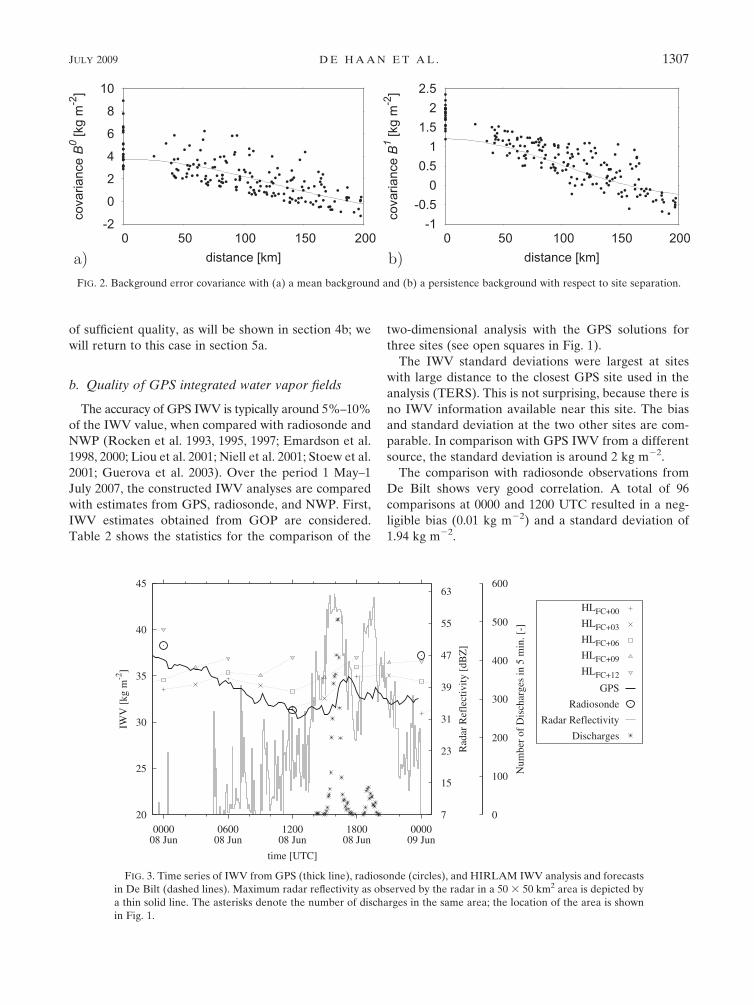
locations). The covariances are shown in Fig. 2a. Also

shown in Fig. 2 is a fit of the background error covari-

ance. Note that the value at zero distance actually is the

sum of the background error and the observation error.

Using this background, an initial analysis xa0 can be

constructed; that is,

x0a(t) 5 f [y(t), IWVmean(t); B0, R]. (6)

In the second step, the background is the initial

analysis as obtained in the first step (using background

error covariances B0). The time series of the differences

between this analysis and observations 15 min later are

used to determine the background error covariances B1:

B1ij 5 [x0

a,i(t)� yi(t 1 159)][x0a, j(t)� yj(t 1 159)]T, (7)

where x0a,i(t) is the vector of initial analyses interpolated

to locations at which the observations were recorded.

The results are shown in Fig. 2b. The background error

covariances B1 will be used to calculate the real-time

variational analysis xa; that is,

xa(t) 5 f [y(t), xa(t � 159); B1, R]. (8)

The period over which the background error covari-

ances are estimated runs from January to July of 2007.

The background error covariance in the first step has

values ranging from 22 to 6 kg m22 for distances larger

than zero. This is due to the coarse background field

used, which is a single value for the whole region. The

background error covariances decrease to values ranging

from 21 to 1.5 kg m22 in the second step. This decrease

is the result of a better background estimate, although

persistence is used and no forward model is applied. The

estimate of the observation errors, which can be deduced

from the covariances at zero distances, ranges from 1 to

1.5 kg m22. These values have been observed in earlier

studies and show that the method used here results

in good covariances (Rocken et al. 1993, 1995, 1997;

Emardson et al. 1998, 2000; Liou et al. 2001; Niell et al.

2001; Stoew et al. 2001; Guerova et al. 2003).

4. Validation of integrated water fields

In this section the validation of IWV analysis fields is

discussed. First, an example is presented that shows that

the sudden development of a thunderstorm could not be

forecast from time series information alone. Next, the

quality of the IWV analysis fields is investigated.

a. Time series analysis

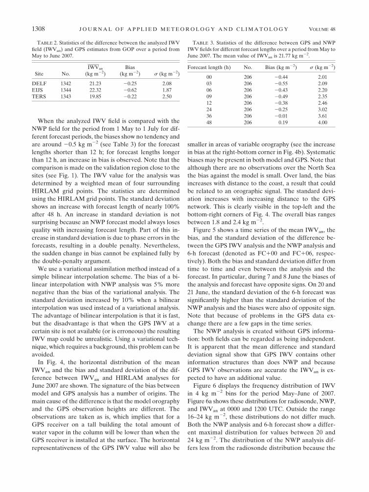
An example of the data described previously is shown

in Fig. 3 for 8 June 2007. GPS IWV and HIRLAM IWV

are observed at the GPS site in the center of the square

in Fig. 1. The difference in temporal resolution is ob-

vious. Figure 3 shows large deviations between GPS

IWV and HIRLAM IWV that sometimes increase with

forecast time; this has been noted before (see, e.g.,

Smith et al. 2007; de Haan and Barlag 2004, chapter 6.1).

Furthermore, the GPS IWV and radiosonde observa-

tion are close except at 0000 UTC 9 June, for which

time it deviates from both the HIRLAM analyses

and the GPS value. In general, HIRLAM analyses are

close to the observed GPS IWV (except the analysis at

0000 UTC 8 June). The forecasts show much larger dis-

crepancies, especially the forecasts valid at 1200 UTC. At

this time the GPS and radiosonde match perfectly.

From 1500 to 1600 UTC, maximum radar reflectivity is

observed up to nearly 63 dBZ (observed in a period of

5 min) in the area of 50 3 50 km2. A reflectivity of

55 dBZ corresponds to a rain rate of approximately

100 mm h21. In the same period, a maximum of 500 dis-

charges in 5 min is observed. These occurrences over-

lap a local increase of IWV from approximately 31 to

35 kg m22. This increase in IWV was present in the

HIRLAM forecast started at 0600 and 1200 UTC. The

first forecast started with a too-large amount of IWV,

and the second overestimated the increase from 1500 to

1800 UTC.

Figure 3 shows an increase in IWV, but this happens

after the time during which the thunderstorm appeared.

The occurrence of the lightning around 1600 UTC

seems to match with the increase in IWV. From the time

series shown in Fig. 3 the thunderstorm event cannot be

explained; two-dimensional representation may reveal

the explanation for the occurrence of this thunderstorm

when the observed two-dimensional water vapor field is


of sufficient quality, as will be shown in section 4b; we

will return to this case in section 5a.

b. Quality of GPS integrated water vapor fields

The accuracy of GPS IWV is typically around 5%–10%

of the IWV value, when compared with radiosonde and

NWP (Rocken et al. 1993, 1995, 1997; Emardson et al.

1998, 2000; Liou et al. 2001; Niell et al. 2001; Stoew et al.

2001; Guerova et al. 2003). Over the period 1 May–1

July 2007, the constructed IWV analyses are compared

with estimates from GPS, radiosonde, and NWP. First,

IWV estimates obtained from GOP are considered.

Table 2 shows the statistics for the comparison of the

two-dimensional analysis with the GPS solutions for

three sites (see open squares in Fig. 1).

The IWV standard deviations were largest at sites

with large distance to the closest GPS site used in the

analysis (TERS). This is not surprising, because there is

no IWV information available near this site. The bias

and standard deviation at the two other sites are com-

parable. In comparison with GPS IWV from a different

source, the standard deviation is around 2 kg m22.

The comparison with radiosonde observations from

De Bilt shows very good correlation. A total of 96

comparisons at 0000 and 1200 UTC resulted in a neg-

ligible bias (0.01 kg m22) and a standard deviation of

1.94 kg m22.

FIG. 3. Time series of IWV from GPS (thick line), radiosonde (circles), and HIRLAM IWV analysis and forecasts

in De Bilt (dashed lines). Maximum radar reflectivity as observed by the radar in a 50 3 50 km2 area is depicted by

a thin solid line. The asterisks denote the number of discharges in the same area; the location of the area is shown

in Fig. 1.

FIG. 2. Background error covariance with (a) a mean background and (b) a persistence background with respect to site separation.

JULY 2009 D E H A A N E T A L . 1307

When the analyzed IWV field is compared with the

NWP field for the period from 1 May to 1 July for dif-

ferent forecast periods, the biases show no tendency and

are around 20.5 kg m22 (see Table 3) for the forecast

lengths shorter than 12 h; for forecast lengths longer

than 12 h, an increase in bias is observed. Note that the

comparison is made on the validation region close to the

sites (see Fig. 1). The IWV value for the analysis was

determined by a weighted mean of four surrounding

HIRLAM grid points. The statistics are determined

using the HIRLAM grid points. The standard deviation

shows an increase with forecast length of nearly 100%

after 48 h. An increase in standard deviation is not

surprising because an NWP forecast model always loses

quality with increasing forecast length. Part of this in-

crease in standard deviation is due to phase errors in the

forecasts, resulting in a double penalty. Nevertheless,

the sudden change in bias cannot be explained fully by

the double-penalty argument.

We use a variational assimilation method instead of a

simple bilinear interpolation scheme. The bias of a bi-

linear interpolation with NWP analysis was 5% more

negative than the bias of the variational analysis. The

standard deviation increased by 10% when a bilinear

interpolation was used instead of a variational analysis.

The advantage of bilinear interpolation is that it is fast,

but the disadvantage is that when the GPS IWV at a

certain site is not available (or is erroneous) the resulting

IWV map could be unrealistic. Using a variational tech-

nique, which requires a background, this problem can be

avoided.

In Fig. 4, the horizontal distribution of the mean

IWVan and the bias and standard deviation of the dif-

ference between IWVan and HIRLAM analyses for

June 2007 are shown. The signature of the bias between

model and GPS analysis has a number of origins. The

main cause of the difference is that the model orography

and the GPS observation heights are different. The

observations are taken as is, which implies that for a

GPS receiver on a tall building the total amount of

water vapor in the column will be lower than when the

GPS receiver is installed at the surface. The horizontal

representativeness of the GPS IWV value will also be

smaller in areas of variable orography (see the increase

in bias at the right-bottom corner in Fig. 4b). Systematic

biases may be present in both model and GPS. Note that

although there are no observations over the North Sea

the bias against the model is small. Over land, the bias

increases with distance to the coast, a result that could

be related to an orographic signal. The standard devi-

ation increases with increasing distance to the GPS

network. This is clearly visible in the top-left and the

bottom-right corners of Fig. 4. The overall bias ranges

between 1.8 and 2.4 kg m22.

Figure 5 shows a time series of the mean IWVan, the

bias, and the standard deviation of the difference be-

tween the GPS IWV analysis and the NWP analysis and

6-h forecast (denoted as FC100 and FC106, respec-

tively). Both the bias and standard deviation differ from

time to time and even between the analysis and the

forecast. In particular, during 7 and 8 June the biases of

the analysis and forecast have opposite signs. On 20 and

21 June, the standard deviation of the 6-h forecast was

significantly higher than the standard deviation of the

NWP analysis and the biases were also of opposite sign.

Note that because of problems in the GPS data ex-

change there are a few gaps in the time series.

The NWP analysis is created without GPS informa-

tion: both fields can be regarded as being independent.

It is apparent that the mean difference and standard

deviation signal show that GPS IWV contains other

information structures than does NWP and because

GPS IWV observations are accurate the IWVan is ex-

pected to have an additional value.

Figure 6 displays the frequency distribution of IWV

in 4 kg m22 bins for the period May–June of 2007.

Figure 6a shows these distributions for radiosonde, NWP,

and IWVan at 0000 and 1200 UTC. Outside the range

16–24 kg m22, these distributions do not differ much.

Both the NWP analysis and 6-h forecast show a differ-

ent maximal distribution for values between 20 and

24 kg m22. The distribution of the NWP analysis dif-

fers less from the radiosonde distribution because the

TABLE 2. Statistics of the difference between the analyzed IWV

field (IWVan) and GPS estimates from GOP over a period from

May to June 2007.

Site No.

IWVan

(kg m22)

Bias

(kg m22) s (kg m22)

DELF 1342 21.23 20.25 2.08

EIJS 1344 22.32 20.62 1.87

TERS 1343 19.85 20.22 2.50

TABLE 3. Statistics of the difference between GPS and NWP

IWV fields for different forecast lengths over a period from May to

June 2007. The mean value of IWVan is 21.77 kg m22.

Forecast length (h) No. Bias (kg m22) s (kg m22)

00 206 20.44 2.01

03 206 20.55 2.09

06 206 20.43 2.20

09 206 20.49 2.35

12 206 20.38 2.46

24 206 20.25 3.02

36 206 20.01 3.61

48 206 0.19 4.00


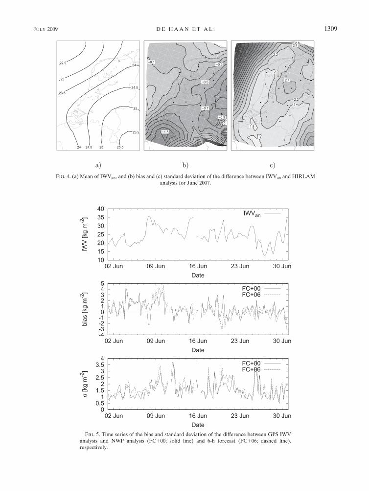
FIG. 4. (a) Mean of IWVan, and (b) bias and (c) standard deviation of the difference between IWVan and HIRLAM

analysis for June 2007.

FIG. 5. Time series of the bias and standard deviation of the difference between GPS IWV

analysis and NWP analysis (FC100; solid line) and 6-h forecast (FC106; dashed line),

respectively.

JULY 2009 D E H A A N E T A L . 1309

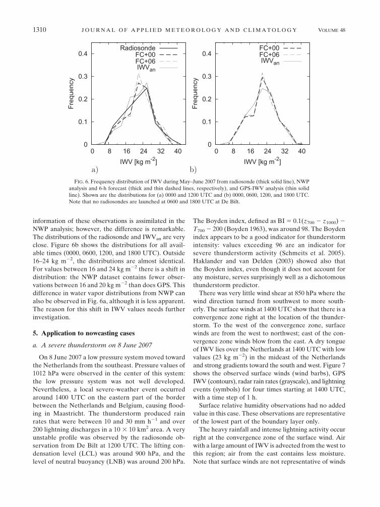
information of these observations is assimilated in the

NWP analysis; however, the difference is remarkable.

The distributions of the radiosonde and IWVan are very

close. Figure 6b shows the distributions for all avail-

able times (0000, 0600, 1200, and 1800 UTC). Outside

16–24 kg m22, the distributions are almost identical.

For values between 16 and 24 kg m22 there is a shift in

distribution: the NWP dataset contains fewer obser-

vations between 16 and 20 kg m22 than does GPS. This

difference in water vapor distributions from NWP can

also be observed in Fig. 6a, although it is less apparent.

The reason for this shift in IWV values needs further

investigation.

5. Application to nowcasting cases

a. A severe thunderstorm on 8 June 2007

On 8 June 2007 a low pressure system moved toward

the Netherlands from the southeast. Pressure values of

1012 hPa were observed in the center of this system:

the low pressure system was not well developed.

Nevertheless, a local severe-weather event occurred

around 1400 UTC on the eastern part of the border

between the Netherlands and Belgium, causing flood-

ing in Maastricht. The thunderstorm produced rain

rates that were between 10 and 30 mm h21 and over

200 lightning discharges in a 10 3 10 km2 area. A very

unstable profile was observed by the radiosonde ob-

servation from De Bilt at 1200 UTC. The lifting con-

densation level (LCL) was around 900 hPa, and the

level of neutral buoyancy (LNB) was around 200 hPa.

The Boyden index, defined as BI 5 0.1(z700 2 z1000) 2

T700 2 200 (Boyden 1963), was around 98. The Boyden

index appears to be a good indicator for thunderstorm

intensity: values exceeding 96 are an indicator for

severe thunderstorm activity (Schmeits et al. 2005).

Haklander and van Delden (2003) showed also that

the Boyden index, even though it does not account for

any moisture, serves surprisingly well as a dichotomous

thunderstorm predictor.

There was very little wind shear at 850 hPa where the

wind direction turned from southwest to more south-

erly. The surface winds at 1400 UTC show that there is a

convergence zone right at the location of the thunder-

storm. To the west of the convergence zone, surface

winds are from the west to northwest; east of the con-

vergence zone winds blow from the east. A dry tongue

of IWV lies over the Netherlands at 1400 UTC with low

values (23 kg m22) in the mideast of the Netherlands

and strong gradients toward the south and west. Figure 7

shows the observed surface winds (wind barbs), GPS

IWV (contours), radar rain rates (grayscale), and lightning

events (symbols) for four times starting at 1400 UTC,

with a time step of 1 h.

Surface relative humidity observations had no added

value in this case. These observations are representative

of the lowest part of the boundary layer only.

The heavy rainfall and intense lightning activity occur

right at the convergence zone of the surface wind. Air

with a large amount of IWV is advected from the west to

this region; air from the east contains less moisture.

Note that surface winds are not representative of winds

FIG. 6. Frequency distribution of IWV during May–June 2007 from radiosonde (thick solid line), NWP

analysis and 6-h forecast (thick and thin dashed lines, respectively), and GPS-IWV analysis (thin solid

line). Shown are the distributions for (a) 0000 and 1200 UTC and (b) 0000, 0600, 1200, and 1800 UTC.

Note that no radiosondes are launched at 0600 and 1800 UTC at De Bilt.


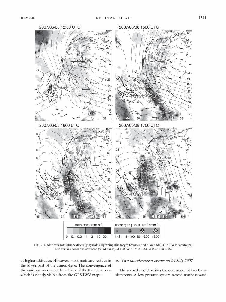
at higher altitudes. However, most moisture resides in

the lower part of the atmosphere. The convergence of

the moisture increased the activity of the thunderstorm,

which is clearly visible from the GPS IWV maps.

b. Two thunderstorm events on 20 July 2007

The second case describes the occurrence of two thun-

derstorms. A low pressure system moved northeastward

FIG. 7. Radar rain-rate observations (grayscale), lightning discharges (crosses and diamonds), GPS IWV (contours),

and surface wind observations (wind barbs) at 1200 and 1500–1700 UTC 8 Jun 2007.

JULY 2009 D E H A A N E T A L . 1311

through the English Channel toward the Netherlands on

20 July 2007. A warm front, on the east side of the

system with an east–west direction, preceded the low

pressure system. On the west side of the low pressure

center an occulted front moved to the west. At 1800 UTC

this system was situated over the mideast of the

Netherlands. The radiosonde profile from De Bilt at

1200 UTC showed an almost completely saturated

profile with an LCL at 950 hPa and an LNB around

290 hPa. The Boyden index was 96, which implies a

moderate chance of severe thunderstorms. Surface

winds ahead of the low pressure system were from the

northeast; behind this system southwest winds were

observed. A water vapor maximum traveled from south

to north over the Netherlands, entering the south at

1000 UTC and leaving the region at 1900 UTC. The

maximum value was over 40 kg m22. A large thunder-

storm moved in the same direction, although with a

higher group velocity; the maximum activity occurred

east of the water vapor maximum. The thunderstorm

entered the Netherlands at 1100 UTC and had exited

the country by 1700 UTC. At that time a second line

of thunderstorms developed over the middle of the

Netherlands; the position of this thunderstorm coincides

locally with water vapor contours at the location where

the water vapor gradients are large. In Fig. 8, the ob-

served surface winds (wind barbs), GPS IWV (contours),

radar rain rates (grayscale), and lightning events

(symbols) for four times, with a time step of 2 h, are

shown. Also, in this case the surface relative humidity

observations showed no signal for the occurrence of

the thunderstorms.

It appears that the intense lightning of the first

thunderstorm occurred to the east of the water vapor

maximum. The thunderstorm overtook the water vapor

maximum and then weakened. The second thunder-

storm developed in a zone of surface wind convergence

that was present more than 2 h prior. Moist air was

advected from the maximum (which lies north of the

convergence zone) to this region, resulting in an in-

crease in the intensity of the thunderstorm (Banacos

and Schultz 2005). Thus again, the IWV fields provide

useful information.

c. Intense line of lightning on 31 May 2008

The last case presented here describes the occurrence

of an intense line of thunderstorms that were aligned

with (or through) the general atmospheric flow. On

31 May 2008 a moderate high pressure system was

present over western Europe, extending from England

to Germany. Radiosonde observations at 1200 UTC

31 May show a surface wind from the northwest while

above 800 hPa the wind veered toward the east. This

profile had a Boyden index of 94 and was unsaturated.

At 0000 UTC 1 June 2008 the radiosonde launch showed

that the winds at high altitude where still from the east

while in the boundary layer the winds were from the

southeast. The profile was almost completely saturated

from 900 up to 400 hPa. The Boyden index was again

around 94.

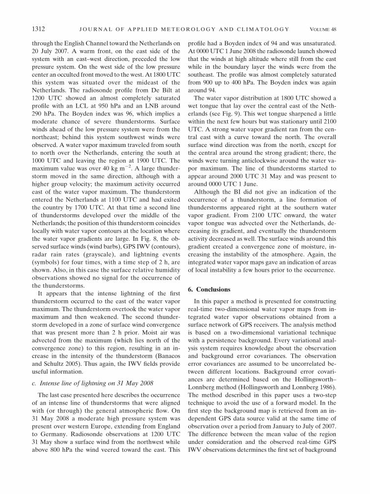
The water vapor distribution at 1800 UTC showed a

wet tongue that lay over the central east of the Neth-

erlands (see Fig. 9). This wet tongue sharpened a little

within the next few hours but was stationary until 2100

UTC. A strong water vapor gradient ran from the cen-

tral east with a curve toward the north. The overall

surface wind direction was from the north, except for

the central area around the strong gradient; there, the

winds were turning anticlockwise around the water va-

por maximum. The line of thunderstorms started to

appear around 2000 UTC 31 May and was present to

around 0000 UTC 1 June.

Although the BI did not give an indication of the

occurrence of a thunderstorm, a line formation of

thunderstorms appeared right at the southern water

vapor gradient. From 2100 UTC onward, the water

vapor tongue was advected over the Netherlands, de-

creasing its gradient, and eventually the thunderstorm

activity decreased as well. The surface winds around this

gradient created a convergence zone of moisture, in-

creasing the instability of the atmosphere. Again, the

integrated water vapor maps gave an indication of areas

of local instability a few hours prior to the occurrence.

6. Conclusions

In this paper a method is presented for constructing

real-time two-dimensional water vapor maps from in-

tegrated water vapor observations obtained from a

surface network of GPS receivers. The analysis method

is based on a two-dimensional variational technique

with a persistence background. Every variational anal-

ysis system requires knowledge about the observation

and background error covariances. The observation

error covariances are assumed to be uncorrelated be-

tween different locations. Background error covari-

ances are determined based on the Hollingsworth–

Lonnberg method (Hollingsworth and Lonnberg 1986).

The method described in this paper uses a two-step

technique to avoid the use of a forward model. In the

first step the background map is retrieved from an in-

dependent GPS data source valid at the same time of

observation over a period from January to July of 2007.

The difference between the mean value of the region

under consideration and the observed real-time GPS

IWV observations determines the first set of background


error covariances. Next, these background error covari-

ances are used together with real-time observations to

obtain an analysis map. This map is then used to de-

termine the background error covariances with real-

time observation 15 min later.

The maps are validated with HIRLAM IWV analysis

and forecast maps and with radiosonde observations.

The mean difference between radiosonde and GPS

IWV maps is negligible, and the standard deviation is

less than 2 kg m22. The bias between HIRLAM and

FIG. 8. As in Fig. 7, but at 1000, 1300, 1500, and 1700 UTC 20 Jul 2007.

JULY 2009 D E H A A N E T A L . 1313

GPS IWV is between 0.4 and 0.6 kg m22, and the

standard deviation increases from 2 to 4 kg m22 with

increasing forecast length to 48 h. This is due to the fact

that the forecast skill decreases with increasing forecast

length. The horizontal distribution of the difference

between 1 month of HIRLAM IWV and GPS IWV

shows a small signal of increasing bias with increasing

distance to the coast. The standard deviation increases

dramatically with increasing distance from the obser-

vation network. Histograms of the IWV values of

HIRLAM are different from those observed with ra-

diosonde and GPS. The occurrence of IWV values

FIG. 9. As in Fig. 7, but at 1800 and 2000–2200 UTC 31 May 2008.


around 16 kg m22 and around 20 kg m22 for HIRLAM

seems to be shifted toward the higher values relative to

both radiosonde and GPS. The statistics are represen-

tative for a larger period, because GPS IWV observa-

tions have a standard deviation of 5%–10% over all

seasons when compared with radiosondes, water vapor

radiometer observations, and NWP.

By examining three cases, the additional value of the

real-time GPS IWV maps for nowcasting is illustrated.

All cases show that the convergence of moist air con-

tains information about the location of developing thun-

derstorms. In the future we plan to perform an evaluation

of real-time GPS IWV maps over a whole season.

Altogether it is concluded that the real-time GPS

IWV maps constructed using a two-dimensional varia-

tional method are of good quality and can be helpful for

nowcasting of severe thunderstorms.

Acknowledgments. The authors thank the GPS data

providers within the EUREF Permanent Network

(EPN) and the International GNSS Service (IGS) for

giving access to their data and products. Special thanks

are given to the Bundesamt fur Kartographie und

Geodasie (BKG), Frankfurt am Main, Germany, for

access to the real-time GPS data (NTRIP). The devel-

opment of the real-time processing scheme of GPS data

was sponsored by The Netherlands Agency for Aero-

space Programmes (NIVR).

REFERENCES

Baltink, H. K., H. van der Marel, and A. G. A. van der Hoeven,

2002: Integrated atmospheric water vapor estimates from a

regional GPS network. J. Geophys. Res., 107, 4025, doi:10.1029/

2000JD000094.

Banacos, P., and D. Schultz, 2005: The use of moisture flux con-

vergence in forecasting convective initiation: Historical and

operational perspectives. Wea. Forecasting, 20, 351–366.

Beekhuis, H., and I. Holleman, 2004: Upgrade and evaluation of a

lightning detection system. Proc. Int. Lightning Detection

Conf. 2004, Helsinki, Finland, Vaisala, 17 pp.

Bevis, M., S. Businger, S. Chiswell, T. A. Herring, R. A. Anthes,

C. Rocken, and R. H. Ware, 1994: GPS meteorology: Map-

ping zenith wet delays onto precipitable water. J. Appl.

Meteor., 33, 379–386.

Boyden, C. J., 1963: A simple instability index for use as a synoptic

parameter. Meteor. Mag., 92, 198–210.

Daley, R., 1991: Atmospheric Data Analysis. 2nd ed. Cambridge

University Press, 457 pp.

Davis, J., T. Herring, I. Shapiro, A. Rogers, and G. Elgered, 1985:

Geodesy by radio interferometry: Effects of atmospheric

modeling errors on estimates of baseline length. Radio Sci.,

20, 1593–1607.

de Haan, S., 2006: Measuring atmospheric stability with GPS.

J. Appl. Meteor. Climatol., 45, 467–475.

——, and S. J. M. Barlag, 2004: Time series. Final Report of

COST716 Working Group 1, G. Elgered et al., Eds., European

Union, 98–103.

——, H. van der Marel, and S. J. M. Barlag, 2002: Comparison of

GPS slant delay measurements to a numerical model: Case

study of a cold front passage. Phys. Chem. Earth, 27, 317–322.

——, S. J. M. Barlag, H. K. Baltink, and F. Debie, 2004: Synergetic

use of GPS water vapor and Meteosat images for synoptic

weather forecasting. J. Appl. Meteor., 43, 514–518.

Doviak, R. J., and D. S. Zrni�c, 1993: Doppler Radar and Weather

Observations. 2nd ed. Academic Press, 562 pp.

Emardson, T. R., G. Elgered, and J. M. Johanson, 1998: Three

months of continuous monitoring of atmospheric water

vapor with a network of global positioning system receivers.

J. Geophys. Res., 103, 1807–1820.

——, J. M. Johanson, and G. Elgered, 2000: The systematic be-

haviour of water vapor estimates using four years of GPS ob-

servations. Trans. IEEE Geosci. Remote Sens., GE-3, 324–329.

Guerova, G., E. Brockmann, J. Quiby, F. Schubiger, and C. Mat-

zler, 2003: Validation of NWP mesoscale models with Swiss

GPS network AGNES. J. Appl. Meteor., 42, 141–150.

Haklander, A. J., and A. van Delden, 2003: Thunderstorm pre-

dictors and their forecast skill for the Netherlands. Atmos.

Res., 67–68, 273–299.

Holleman, I., 2005: Quality control and verification of weather radar

wind profiles. J. Atmos. Oceanic Technol., 22, 1541–1550.

——, 2007: Bias adjustment and long-term verification of radar-

based precipitation estimates. Meteor. Appl., 14, 195–203.

——, H. Beekhuis, S. Noteboom, L. Evers, H. W. Haak, H. Falcke,

and L. Bahren, 2006: Validation of an operational lightning

detection system. Proc. Int. Lightning Detection Conf. 2006,

Tucson, AZ, Vaisala, 16 pp. [Available online at http://

www.vaisala.com/files/Validation_of_an_operational_lightning

_detection_system.pdf.]

Hollingsworth, A., and P. Lonnberg, 1986: The statistical structure

of short-range forecast errors as determined from radiosonde

data. Part I: The wind field. Tellus, 38A, 111–136.

Liou, Y. A., Y. T. Teng, T. van Hove, and J. C. Liljegren, 2001:

Comparison of precipitable water observations in the near

tropics by GPS, microwave radiometer, and radiosondes.

J. Appl. Meteor., 40, 5–15.

Macpherson, S. R., G. Deblonde, J. M. Aparicio, and B. Casati,

2007: Impact of ground-based GPS observations on the Ca-

nadian Regional Analysis and Forecast System. Preprints,

11th Symp. on Integrated Observing and Assimilation Systems

for the Atmosphere, Oceans, and Land Surface (IOAS-AOLS),

San Antonio, TX, Amer. Meteor. Soc., 5.5. [Available online at

http://ams.confex.com/ams/pdfpapers/117995.pdf.]

Marshall, J. S., and W. M. Palmer, 1948: The distribution of rain-

drops with size. J. Meteor., 5, 165–166.

Mazany, R. A., S. Businger, S. I. Gutman, and W. Roeder, 2002: A

lightning prediction index that utilizes GPS-integrated pre-

cipitable water vapor. Wea. Forecasting, 17, 1034–1047.

Niell, A. E., A. J. Coster, F. S. Solheim, and V. B. Mendes, 2001:

Comparison of measurements of atmospheric wet delay by

radiosonde, water vapor radiometer, GPS, and VLBI. J. At-

mos. Oceanic Technol., 18, 830–850.

Poli, P., and Coauthors, 2007: Forecast impact studies of zenith

total delay data from European near real-time GPS stations

in Meteo France 4DVAR. J. Geophys. Res., 112, D06114,

doi:10.1029/2006JD007430.

Ray, R. D., 1999: A global ocean tide model from TOPEX/

Poseidon altimetry: GOT99.2. NASA Tech. Memo. 209478,

Goddard Space Flight Center, 58 pp.

Rocken, C., R. Ware, T. van Hove, F. Solheim, C. Alber, J. Johnson,

M. Bevis, and S. Businger, 1993: Sensing atmospheric water

JULY 2009 D E H A A N E T A L . 1315

vapor with the global positioning system. Geophys. Res.

Lett., 20, 2631–2634.

——, T. van Hove, J. Johnson, F. Solheim, R. Ware, M. Bevis,

S. Chiswell, and S. Busingerb, 1995: GPS/STORM—GPS

sensing of atmospheric water vapor for meteorology. J. Atmos.

Oceanic Technol., 12, 468–478.

Rocken, C. R., T. van Hove, and R. H. Ware, 1997: Near real-time

GPS sensing of atmospheric water vapor. Geophys. Res. Lett.,

24, 3221–3224.

Saastamoinen, J., 1972: Atmospheric correction for the tropo-

sphere and stratosphere in radio ranging of satellites. The Use

of Artificial Satellites for Geodesy, Geophys. Monogr., Vol. 15,

Amer. Geophys. Union, 247–251.

Scherneck, H.-G., 1991: A parametrized solid earth tide mode and

ocean loading effects for global geodetic base-line measure-

ments. Geophys. J. Int., 106, 677–694.

Schmeits, M. J., K. J. Kok, and D. H. P. Vogelezang, 2005: Prob-

abilistic forecasting of (severe) thunderstorms in the Nether-

lands using model output statistics. Wea. Forecasting, 20,

134–148.

Smith, T. L., S. I. Gutman, and S. R. Sahm, 2007: Forecast impact

from assimilation of GPS IPW observations into the Rapid

Update Cycle. Mon. Wea. Rev., 135, 2914–2930.

Stoew, B., G. Elgered, and J. M. Johansson, 2001: An assessment

of estimates of integrated water vapour from ground based

GPS data. Meteor. Atmos. Phys., 77, 99–107.

Unden, P., and Coauthors, 2002: HIRLAM-5 scientific documen-

tation. IRLAM Project Tech. Rep., Norrkoping, Sweden,

144 pp. [Available online at http://hirlam.org.]

Vaisala, 2006: Vaisala radiosonde RS92-SGP brochure. Vaisala

Oyj Tech. Rep. Ref. B210358EN-C, Helsinki, Finland, 2 pp.

[Available online at http://www.vaisala.com/.]


real-time water vapor maps from a gps surface network...

Documents