real-time virtual viewpoint generation on the gpu for ... · real-time virtual viewpoint generation...

6/3/2010

1

Real-Time Virtual Viewpoint Generation on the GPU for Scene

Navigation

Presenter: Robert Laganière

CoAuthor: Shanat Kolhatkar

May 31st 2010

Contributions

• Our work brings forth 3 main contributions:

– The calculation of new viewpoints in real-time

using a view morphing algorithm

– The ability to navigate the environment in real-

time through the use of GPU programming

– Enhancing the optical flow to reduce the number

of noticeable artifacts

6/3/2010

2

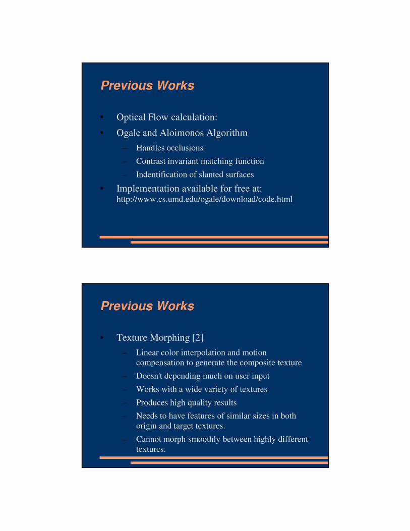
Previous Works

• Optical Flow calculation:

• Ogale and Aloimonos Algorithm

– Handles occlusions

– Contrast invariant matching function

– Indentification of slanted surfaces

• Implementation available for free at: http://www.cs.umd.edu/ogale/download/code.html

Previous Works

• Texture Morphing [2]

– Linear color interpolation and motion

compensation to generate the composite texture

– Doesn't depending much on user input

– Works with a wide variety of textures

– Produces high quality results

– Needs to have features of similar sizes in both

origin and target textures.

– Cannot morph smoothly between highly different

textures.

6/3/2010

3

Previous Works

•

• Termes:

– ci, wj : Color and distance

weights

– Ii: Color map of texture i

– Wij: Displacement map

from texture i to texture j

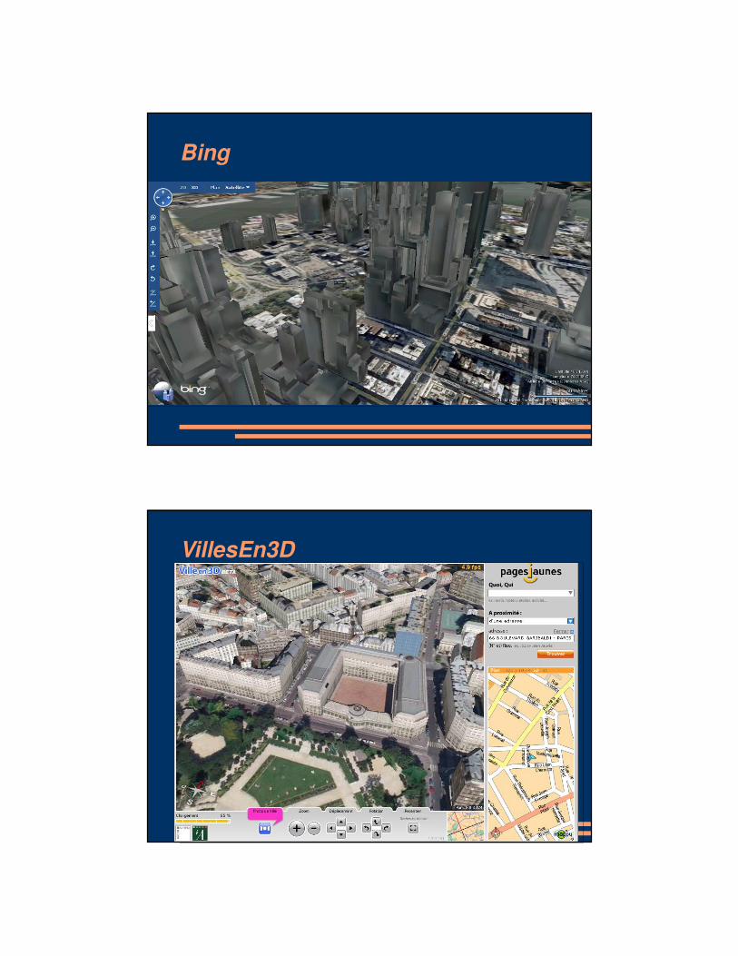
Virtual Navigation Software

• Using panoramas:

– Google Street View

– EveryScape

• Using 3D reconstruction

– Bing

– Google Earth Feature

– VillesEn3D

6/3/2010

4

Bing

The linked image cannot be displayed. The file may have been moved, renamed, or deleted. Verify that the link points to the correct file and location.

VillesEn3DThe linked image cannot be displayed. The file may have been moved, renamed, or deleted. Verify that the link points to the correct file and location.

6/3/2010

5

Google Street View


A Captured Panorama

Google Street View


A Transition Image example

6/3/2010

6

Part 1: Enhancing the Optical Flow

Part 1: The Extended Cube

• An example of the previously used cubic panorama representation



6/3/2010

7


• Description of the extended cube

– Each face is extended a certain number of pixels to

each side during generation

– Goal: Correctly estimate the displacement of a

visual point moving from one face to another. (small displacements)


• Extended Cube exampleThe linked image cannot be displayed. The file may have been moved, renamed, or deleted. Verify that the link points to the correct file and location.

6/3/2010

8


• 3D View of the Extended Cube



• Boundary Handling

– Some displacement vectors are computed twice because they appear on each extended portion of two adjacent faces

– We check which of these two solutions gives the best result by comparing the color neighborhood in both images according to the L2-norm

– The one with the greatest distance is then replaced by the other one


6/3/2010

9


Interpolated image using a cube

Interpolated image using our

extended cube

Part 1: Smoothing The Flow Field

• We assume that the image is static.

– neighboring flow vectors should have a similar

orientation

6/3/2010

10

Part 1: Smoothing The Flow FieldThe linked image cannot be displayed. The file may have been moved, renamed, or deleted. Verify that the link points to the correct file and location.

Original Destination

UncorrectedSmoothed

Part 2: View Interpolation

6/3/2010

11


• Calculate each extended face of the cube independently from the others

• We use the previously calculated dense flow field to interpolate the position of the pixels

• We want the color and the motion to be interpolated jointly thus, our interpolation is

written as:


6/3/2010

12

Part 3: Real-Time Navigation

Part 3: Real-Time Navigation

• Four Components are necessary to achieve Interactive Navigation

– Pre-calculation of the flow

– Multi-Threading

– Buffering

– GPU Implementation of the interpolation

6/3/2010

13

Part 3: Multi-Threading

• Use 3 Threads:

– One thread to handle the graphics calls (in our

architecture, the OpenGL calls)

– One to load the data from the hard drive

– One thread to calculate the interpolated images, which is actually run on the GPU

Part 3: Buffering

• This graph is an example of a possible panorama setting. Let us suppose that our buffer size is 7. If the user is currently at the viewpoint P1, then the buffer is filled with the panoramas and displacement fields of the following viewpoints: P1, P0, P2, P5, P8, P3, P6.


6/3/2010

14

Part 3: GPU Implementation

• Each pixel's interpolation is calculated independently from each other

– we just need the origin and target pixels color values and the flow vectors)

– This makes it a perfect algorithm for GPU

implementation

Part 3: GPU Implementation

• GPU Algorithm

6/3/2010

15

Part 4: Results

Part 4: Results

• On the CPU, we created 20 transition images in 3 seconds. With

our GPU based interpolation scheme, we could generate up to

1000 images in 3 seconds, with identical quality. (We ran our tests on a Pentium M 1.7Ghz with a Radeon Mobility X700)

• The optical flow calculation and correction took up to an hour on

a 320x320 image on an Athlon 64 X2 6000+/3GHz. We ran the

optical flow calculation with an interval for both x and y of [-40;

40] and we set the size of all the neighborhoods in the correction

pass to 11.

6/3/2010

16

Part 4: Results

• Degradation of results with the increase of the distance between the viewpoints

The linked image cannot be displayed. The file may have been moved, renamed, or deleted. Verify that the link points to the correct file and

location.

Step of 1

Step of 2

Step of 3


Step of 3

Step of 2

Step of 1

6/3/2010

17

Part 4: Results

• Smoothingimprovement


Uncorrected

Smoothed

Shades of Gray RMS Origin

Linear

Uncorrected

Smoothed

Ground Truth

Destination

6/3/2010

18

Shades of Gray RMS

Destination

SmoothedUncorrected

Linear

Origin

RMS Values

6/3/2010

19

Conclusion

• New way of interpolating between pairs of panoramas in

real-time using the GPU,

• Navigate inside a scene and achieve a high degree of

realism.

• Main contribution:

– interpolation of intermediate viewpoints of a scene in real-

time using computed optical flow field.

• Except for a few artifacts, our results are of good quality, as

long as the panoramas were taken at reasonable distances

from each other.

References

[1] A. S. Ogale and Y. Aloimonos. A roadmap to the integration of early visual modules. Int. Journal of

Computer Vision.72:9–25, April 2007.

[2] W. Matusik, M. Zwicker, and F. Durant. Texture

design using a simplicial complex of morphable textures. SIGGRAPH, 4:124–125, 2005.

real-time virtual viewpoint generation on the gpu for ... · real-time virtual viewpoint generation...

Documents