real-time trajectory generation for differentially flat systems

INTERNATIONAL JOURNAL OF ROBUST AND NONLINEAR CONTROL

Int. J. Robust Nonlinear Control 8, 995—1020 (1998)

REAL-TIME TRAJECTORY GENERATION FORDIFFERENTIALLY FLAT SYSTEMS

MICHIEL J. VAN NIEUWSTADT AND RICHARD M. MURRAY

Division of Engineering and Applied Science, California Institute of Technology, Pasadena, CA 91125, USA

SUMMARY

This paper considers the problem of real-time trajectory generation and tracking for nonlinear controlsystems. We employ a two-degree-of-freedom approach that separates the nonlinear tracking problem intoreal-time trajectory generation followed by local (gain-scheduled) stabilization. The central problem whichwe consider is how to generate, possibly with some delay, a feasible state space and input trajectory in realtime from an output trajectory that is given online. We propose two algorithms that solve the real-timetrajectory generation problem for differentially flat systems with (possibly non-minimum phase) zerodynamics. One is based on receding horizon point to point steering, the other allows additionalminimization of a cost function. Both algorithms explicitly address the tradeoff between stability andperformance and we prove convergence of the algorithms for a reasonable class of output trajectories. Toillustrate the application of these techniques to physical systems, we present experimental results usinga vectored thrust flight control experiment built at Caltech. A brief introduction to differentially flat systemsand its relationship with feedback linearization is also included. ( 1998 John Wiley & Sons, Ltd.

Key words: flatness; flight control; trajectory generation

1. INTRODUCTION

A large class of industrial and military control problems consist of planning and followinga trajectory in the presence of noise and uncertainty. Examples range from unmanned andremotely piloted airplanes and submarines performing surveillance and inspection tasks, tomobile robots moving on factory floors, to multi-fingered robot hands performing inspection andmanipulation tasks inside the human body under the control of a surgeon. All of these systems arehighly nonlinear and demand accurate performance.

In this paper, we focus on the problem of trajectory generation and tracking for such motioncontrol systems. Roughly speaking, we wish to design a controller that tracks a desired trajectoryfor a set of outputs of the system. We assume that the desired trajectory is not known ahead oftime, so that the controller must perform all operations in ‘real time’. A good prototype example

*Correspondence to: R. M. Murray, Division of Engineering and Applied Science, California Institute of Technology,Pasadena, CA 91125, USA

Contract/grant sponsor: NSFContract/grant number: CMS-9502224Contract/grant sponsor: AFOSRContract/grant number: F49620-95-1-0419

CCC 1049-8923/98/110995—26$17.50( 1998 John Wiley & Sons, Ltd.

for this class of problems is control of an autonomous aircraft tracking a moving target (perhapsa speeding car on the ground or another aircraft). The target’s trajectory provides the desiredtrajectory for the pursuing aircraft. If the target and the controlled system have identicaldynamics, then in principle one can achieve perfect tracking. In general, however, it will not bepossible to exactly track the reference signal, and so we must tradeoff the tracking performancewith the stability of the controlled system.

In order to design a nonlinear controller that approximately tracks a given trajectory, weseparate the problem into two pieces: a trajectory generation block and a feedback compensationblock, as shown in Figure 1.

The purpose of the trajectory generation block is to synthesize a feasible state-space trajectoryfor the system given a desired reference signal. For example, the reference signal might be thedesired position of the centre of mass of an aircraft. This trajectory may or may not be somethingthat can actually be executed by the aircraft, either due to limitations on the actuation system orbecause there does not exist a trajectory in state space that simultaneously satisfies the equationsof motion and gives the desired trajectory for the centre of mass. It is the responsibility of thetrajectory generation block to use this reference signal to generate a feasible state-spacetrajectory, as well as a set of nominal inputs that drive the system along this path.

Given the feasible state-space trajectory, the feedback compensation block is used to correct forany errors due to noise or plant uncertainty (depicted in the figure as a feedback with unknownparameters *). Given the desired state-space trajectory, x

$, the error dynamics can then be

written as a time-varying control system in terms of the state error, e"x!x$. Under the

assumption that the tracking error remains small, we can linearize this time-varying system aboute"0 and stabilize the e"0 state. One method of doing this is to solve the linear quadraticoptimal control problem to obtain the optimal (time-varying) feedback gain for the path. Moreadvanced techniques include the use of linear-time-varying robust synthesis (see, for example,Reference 1 for recent results and a survey of the literature) and the use of linear parametervarying synthesis developed by Packard2 and others.

Figure 1. Two-degree-of-freedom controller design

996 M. J. VAN NIEUWSTADT AND R. M. MURRAY

( 1998 John Wiley & Sons, Ltd. Int. J. Robust Nonlinear Control 8, 995—1020 (1998)

The use of two-degree-of-freedom design techniques is a classical one in the control literature.In the linear setting, two-degree-of-freedom controllers are usually thought of as containinga feedforward compensator (or shaping filter) that modifies the input to the feedbackcompensator. In our context, we do something slightly stronger since we generate a full-state,feasible trajectory and nominal input, and we allow use of the current state in the ‘feedforward’block. This paradigm is also superficially similar to traditional optimal control techniques, whereoptimal control theory is used to generate a feasible trajectory minimizing some cost function anda feedback compensator is used to track this trajectory. However, for the motion controlapplications that we consider, the reference signal is not available ahead of time (as in the exampleof an airplane following a moving target) and the problems are typically high dimensional andnonlinear, making the optimal control problem difficult to solve in real time.

Many modern nonlinear control methodologies can also be viewed as synthesizing controllersthat fall into the two-degree-of-freedom framework. For example, traditional nonlinear trajectorytracking approaches, such as feedback linearization3,4 and nonlinear output regulation,5 areeasily viewed as a feedforward piece and a feedback piece. Both methods use the structure of theplant dynamics to compute a nominal path for the system and then stabilize the trajectory in local(possibly transformed) co-ordinates. Indeed, when the tracking error is small, the primarydifference between the methods is the form of the error correction term: output regulation uses thelinearization of the system about a single equilibrium point; feedback linearization uses a linearcontrol law in an appropriate set of co-ordinates.

In some cases, it is possible only to linearize the input/output response of the system and notthe full-state dynamics. In this case, the feedback linearizing controller specifies only a portion ofthe dynamics of the system. The remaining internal dynamics (zero dynamics) are not specifiedand evolve independently, driven by the inputs required to track the output signal. If the internaldynamics are unstable (non-minimum phase), this technique cannot be used withoutmodification. It is important to note that all of these modern nonlinear approaches rely on theavailability of state feedback in order to generate feedforward commands. Thus, they are nottraditional open-loop feedforward controllers and this difference is crucial to their operation.

A more sophisticated approach for trajectory generation in the presence of internal dynamics isto extend the trajectory for the outputs and their derivatives to a full-state-space trajectory. Onesuch method is reported by Chen and Paden6 and Devasia and Paden,7 who use non-causalinversion for trajectory generation for systems with well-defined, hyperbolic zero dynamics. Themethod of non-causal inversion tries to find a stable solution for the full-state-space trajectory bysteering from the unstable-zero-dynamics manifold to the stable-zero-dynamics manifold. Thenon-causality results from the fact that we first have to get from the origin to the right position onthe unstable zero-dynamics manifold. The solution is found by repeatedly solving a two-pointboundary-value problem for the linearized zero dynamics driven by the desired trajectory. Thisiteration can also be performed in the frequency domain, as shown by Meyer et al.8

Finally, an approach that does not generate a feasible state-space trajectory, but improves onthe output-only trajectory has been explored by Getz et al.9 The method generates anapproximate trajectory for the internal dynamics by following an instantaneous equilibrium forthe internal dynamics. The first- and higher-order derivatives of the internal states are set to zero.Therefore, the total state trajectory is not feasible. Further refinements of this technique can befound in Reference 10.

In this paper we concentrate on a special class of systems, called differentially flat systems, forwhich there is a one-to-one correspondence between trajectories of a set of ‘flat-outputs’ and

997TRAJECTORY GENERATION FOR DIFFERENTIALLY FLAT SYSTEMS


full-state space and input trajectories. Trajectories can be planned in output space and then liftedto the state and input space, through an algebraic mapping. Differentially, flat systems wereintroduced by Fliess et al.11,12 and are ideally suited for trajectory generation tasks. A variety ofexamples have been shown to be differentially flat (or approximately flat) and controllers basedon trajectory generation by interpolation and then closing the loop on the obtained trajectoryhave been developed. These examples include overhead cranes,13,14 cars with trailers,13,15,16conventional aircraft,17,18 induction motors,19,20 active magnetic bearings,21 and chemicalreactors.22,23 An introduction to differentially flat systems, and a description of their relationshipwith feedback linearizable systems, is given in Section 2.

The point of view taken in this paper also exploits differential flatness, but with a strongeremphasis towards real-time trajectory generation and explicit tradeoffs between performance inthe tracking variables and stability of the internal variables. In Section 3 we introduce thereal-time trajectory generation problem and provide two algorithms for tracking a (possiblynon-minimum phase) output. These algorithms are shown to converge for a reasonable class ofoutput trajectories and allow explicit tradeoff between stability and performance. We apply oneof these algorithms to simulations and experiments of a flight control experiment in Section 4. Wedemonstrate that the two-degree-of-freedom techniques advocated in this paper providesignificant improvement over traditional linear controls. Finally, we summarize our results andoutline some directions for future research in Section 5.

2. DIFFERENTIAL FLATNESS

In this section we prove a brief description of differential flatness and compare it with (dynamic)feedback linearization. More details about differentially flat systems can be found in References11, 12, 21 and 24. For an introduction to feedback linearization, see References 25 and 26.

2.1. Differentially flat systems

Differential flatness was originally introduced by Fliess et al.11 in a differentially algebraiccontext and later using Lie—Backlund transformations.12 The important property of flat systemsis that we can find a set of outputs (equal in number to the number of inputs) such that we canexpress all states and inputs in terms of those outputs and their derivatives. More precisely,a nonlinear system

xR "f (x, u), x3Rn, u3Rm

y"h (x), y3Rm (1)

is differentially flat if we can find outputs z3Rm of the form

z"f(x, u, uR ,2 , u(l)) (2)

such that

x"x (z, zR ,2 , z(l))": x (zN )

u"u (z, zR ,2, z(l))": u (zN ) (3)

We call y the tracking outputs and z the flat outputs. These outputs are not necessarily the sameand care must be taken when the tracking outputs result in right half-plane zeros for the



linearized system, in order to avoid exciting instabilities in the internal dynamics. For ease ofnotation, we stack the flat outputs and their derivatives in the flat flag, zN :"(z, zR ,2 , z(l)).

Differentially flat systems are useful in situations where explicit trajectory generation isrequired. Since the behaviour of flat systems is determined by the flat outputs, we can plantrajectories in output space, and then map these to appropriate inputs. A common example isa kinematic car, where the xy position of the rear wheels provides flat outputs.15,16 This impliesthat all feasible trajectories of the system can be determined by specifying only the trajectory ofthe rear wheels. This idea is illustrated in more detail in the following sections.

Differential flatness can also be characterized using tools from exterior differential systems.24In the beginning of this century, the French geometer E. Cartan developed this set of powerfultools for the study of equivalence of systems of differential equations.27~29. Equivalence need notbe restricted to systems to equal dimensions. In particular, a system can be prolonged to a biggersystem on a bigger manifold, and equivalence between these prolongations can be studied. Twosystems that have equivalent prolongations are called absolutely equivalent. Differentially flatsystems can be interpreted as being those systems which are absolutely equivalent to the trivialsystem, i.e. having no dynamic constraints on the free variables.24 This is illustrated in Figure 2.

2.2. Flatness versus feedback linearization

It is easy to show that any (full-state) feedback linearizable system is differentially flat bychoosing the flat output as the feedback linearizing output. Indeed, differential flatness can beshown to be equivalent to dynamic feedback linearization on an open and dense set using a classof invertible dynamic feedbacks.30,31,4,32 Hence, the class of systems which is differentially flat isessentially the same as dynamically feedback linearizable systems (up to some regularityconditions). However, the point of view used in controlling differentially flat systems issubstantially different than feedback linearization: one concentrates on generating feasibletrajectories rather than transforming the system into a single linear system. Consistent with the

Figure 2. Differential flatness and absolute equivalence. A system xR "f (x, u) is said to be differentially flat if the solutionsare in one-to-one equivalence with the solutions of the trivial system z(t)3M (no dynamics)



two-degree-of-freedomparadigm discussed in the introduction, a (scheduled) linear controller canthen be used to maintain stability of the system around the generated trajectory. This has theadvantage of allowing the local control design to be performed in the original co-ordinates for thesystem, where the various weights and other characteristics of the controller can be specified morenaturally (see, for example, Reference 33).

To illustrate this viewpoint, consider the feedback linearization problem for a singleinput—single output nonlinear control system

xR "f (x)#g(x)u

y"h(x)

Suppose that the output y has relative degree n, so that the system is full-state linearizable. Thenthe dynamics of the system can be transformed to a linear system using a state transformationm"/ (x) and an input transformation u"a (x)#b (x)v where m3Rn is the new state vector andv is the new input. The functions a(x) and b (x) are determined using repeated Lie derivatives ofthe output function (see Reference 26). A standard control law for tracking a desired trajectory iny is one of the form

u"a (x)#b (x)(y(n)$#K (m!m

$)) (4)

where y$( ) ) is the desired output trajectory and m

$is determined by differentiating the desired

output (see Reference 26) for a more complete description).The control law in equation (4) can be viewed as a two-degree-of-freedom controller by slightly

rearranging terms

u"(a(x)#b (x)(y(n)$

)hggiggj

feedforward

#b (x)K (m!m$)

hggiggjfeedback

The feedforward terms are the inputs that are required in order to track the trajectory; thefeedback terms are used to correct any errors due to system uncertainty. Note that the‘feedforward’ controller makes use of the current state of information as well as the desired outputsignal, y

$.

Treating the system as being differentially flat instead of feedback linearizable, a controller fortrajectory tracking would take the form

u"(a (x, zN$)#b (x, zN

$)z(n)

$) #K(x, zN

$) (x!x

d(zN

$)) (5)

There are several differences between this controller and the feedback linearizing controller. First,the nominal inputs are allowed to depend on both the current state and the flat flag, depending onhow one implements certain computations. Thus, the entire trajectory can be computed in a trulyopen-loop fashion (as in optimal control) or the current state can be used (as in feedbacklinearization). Second, feedback of the error term in the feedback linearizing controller inverts thecoupling function b(x). This can lead to numerical problems if b(x) is near singularities or thesystem has substantial uncertainty. In contrast, the controller in equation (5) uses a scheduled gain,allowing tradeoffs between performance and input magnitude to be varied depending on theoperating conditions. Finally, as we show in the sequel, the flatness based controller allows numericalmethods to be used for trajectory generation, rather than requiring symbolic computations.

Additional differences between flatness and feedback linearization are evident when theoutputs that one wants to track are different than the flat outputs. In this case, standard I/O



linearization techniques can fail if the zero dynamics of the system are unstable (non-minimumphase). And even if the zero dynamics are stable, it is possible that the controller may cause theinternal motion to have unacceptably large transient performance. The flatness based controllerswhich we develop in the next section avoid this problem by allowing an explicit tradeoff betweenthe trajectory tracking performance and the stability of the internal motions (see Reference 34 fora more complete discussion of this point).

2.3. Examples

In this subsection we give various examples of mechanical systems that are flat. Additionalexamples and characterizations of flat systems can be found in References 13, 35—38 and 16.

Example 1 (rolling penny)

Consider the motion of a rolling penny, as shown in Figure 3. Let (x1, x

2) represent the xy

position of the penny on the plane, x3

represent the heading angle of the penny relative to a fixedline on the plane, and x

4represent the rotational velocity of the angle of Lincoln’s head, i.e. the

rolling velocity. We restrict x33[0,n) since we cannot distinguish between a positive rolling

velocity x4

at a heading angle x3

and a negative rolling velocity at a heading angle x3#n.

The dynamics of the penny can be written as

xR1"cos x

3x4, xR

2"sinx

3x4, xR

3"x

5, xR

4"u

1, xR

5"u

2(6)

where x5"xR

3is the velocity of the heading angle. The controls u

1and u

2correspond to the

torques around the rolling and heading axes.This system is differentially flat using the outputs x

1and x

2plus knowledge of time. Given

x1

and x2, we can use the first two equations to solve uniquely for x

3and x

4. Then given these

three variables plus time, we can solve for all other variables in the system by differentiation withrespect to time.

Example 2 (planar ducted fan)

Consider the motion of the planar, vectored thrust vehicle shown in Figure 4. This systemconsists of a rigid body with body fixed forces and is a simplified model for the Caltech ducted fandescribed in Reference 39.

The ducted fan is mounted on a stand with a counterweight that moves in as the fan moves up.This results in inertial masses m

xand m

yin the x and y direction, respectively, that change with the

Figure 3. Rolling penny



Figure 4. Planar ducted fan engine. Thrust is vectored by moving the flaps at the end of the duct, as shown on the right

y co-ordinate. We do not take the variation of these inertial masses with y into account but taketheir value around hover. The counterweight also results in an effective weight m

'different than

the inertial masses in x and y direction. We can apply any force on the center of mass by adjustingthe magnitude and the direction of the thrust, or equivalently by commanding the parallel andperpendicular thrust. After shifting the control variables to compensate for gravity,u2Pu

2#m

'g, the equations of motion are

Am

xx~

myy

Jh® B"Acos h !sin h

sin h cos h

r 0 B A u1

u2#m

'gB#A

0

!m'g

0 B (7)

where (x, y) are the co-ordinates centre of the centre of mass, h is the angle with the vertical, u1

isthe force perpendicular to the fan shroud, u

2is the force parallel to the fan shroud, r is the distance

between the centre of mass and the point where the force is applied, g is the gravitational constant,m

x, m

yis the inertial mass of the fan in the (x, y) direction, respectively, m

'g is the weight of the fan,

and J is the moment of inertia. The tracking outputs are the (x, y) co-ordinates of the centre ofmass. Analogous to References 7 and 18, the flat outputs are

x&"x!

J

mxr

sin h, y&"y#

J

myr

cos h (8)

Note that these outputs are not fixed in body co-ordinates. The variable h can be expressed interms of the flat outputs as

tan h"!m

xx~&

myy~&#m

'g

(9)

From h and the flat outputs we can find the other states and the inputs.

Example 3 (simplified helicopter model )

Consider the simplified helicopter depicted in Figure 5. At some level of abstraction we canlook at the helicopter as a rigid body actuated by the thrust of the main rotor and the tail rotor.



Figure 5. Simplified helicopter

The tail rotor exerts a thrust along the body y-axis and a torque along the body z-axis. Thetail rotor force is small compared to the thrust of the main rotor and we neglect it. Themain thrust is roughly aligned with the body z-axis. We can measure the X½Z Eulerangles (/, h,t). The tail rotor torque q

"and the main thrust ¹

"then both act along the body

z-axis and can be transformed to spatial co-ordinates by rotations about the y and x-axisabout angles h and /, respectively. The subscript b indicates that the vector is in bodyco-ordinates, the subscript s indicates spatial co-ordinates. Note that according to aerodynamicconvention the z-axis is positive pointing down, hence ¹

"(0 is a thrust upward. Writing (x, y, z)

for the centre of mass in spatial co-ordinates, the rigid body equations for the model helicopterthen take the form

Amx~

my~

mz~

Jt® B"A¹"sin h

!¹"cos h sin/

¹"cos/ cos h#mg

q"cos/ cos h B (10)

where m is the mass of the helicopter, J is the moment of inertia about the z-axis, and g is thegravitational acceleration. Note that we have no direct control over roll (/) and pitch (h) but onlythrough left—right (aileron) and fore-aft (elevator) cyclic control, respectively (see Reference 34 formore details). The thrust ¹

"and the torque q

"are real control inputs, the pitch angle h and the roll

angle / are pseudo-inputs.The system of rigid body equations (10) is flat since from (x, y, z,t) we can recover the inputs

(¹", q

") and pseudo-inputs (/,h)

D¹"D2"m2(x~ 2#y~ 2#(z~ !g)2)

h"arcsinmx~¹"



h"!arcsinmy~

¹"cos h

Dq"D"

t®J cos/ cos h

(11)

We cannot determine the sign of ¹", since flying right-side up with positive thrust cannot be

distinguished from flying upside down with negative thrust. We will assume that the helicopteralways flies right-side up.

3. REAL-TIME TRAJECTORY GENERATION

In this section we will try to come to meaningful definition of the real-time trajectory generationproblem and present some algorithms for generating feasible trajectories in real time, along withtheir proofs of convergence.

3.1. Trajectory tracking: definition and limitations

The notion of ‘real time’ is somewhat ill-defined and must be considered relative to the physicalprocess under consideration. In our case we reference the time scale to the rate at which thereference signal is updated. A real-time computation will therefore be one that can be performedfaster than the reference update. As before, we consider nonlinear systems of the form

xR "f (x, u), x3Rn, u3Rm

y"h (x), y3Rm (12)

Usually, control objectives are stated as performance criteria subject to stability. For real-timetrajectory generation we only have a finite-time history of the desired trajectory available, andtherefore stability as defined in an infinite-time horizon does not make sense. Instead, we cancapture the notion of stability as some norm bound on the internal dynamics generated whenfollowing a desired trajectory. The ‘performance under stability’ requirement then translates tominimizing a weighted norm between tracking error and magnitude of the internal dynamics. Inagreement with H= control theory we take this norm to be the ¸

2norm on a finite-time interval.

This leads to the following cost to be minimized at each time instant

Pt

t~T$

(h(x)!y$(s))*(h(x)!y

$(s))#jK(x, u) ds (13)

where K is an appropriate penalty on the internal dynamics, and ¹$defines the time horizon, or

the delay with which the trajectory is generated.This formulation allows a tradeoff between performance and stability, as seen in References 34

and 40. We can increase stability at the expense of performance by increasing the penalty on theinternal dynamics (i.e. j). Since we have to minimize the cost in equation (13) at every time instant,we need to do this subject to fixed initial conditions, namely, the state that we happen to be at.

There are theoretical limits to the tracking performance that can be obtained in systems withunstable zero dynamics, as was shown in a theorem by Grizzle et al.41 that we repeat here forcompleteness. Recall that a left inverse of a system & is a system &

Lthat reconstructs the unique

input that generates a given output of &, given that output and the initial state (see Reference 26).



Theorem 1 (Reference 26)

Suppose the nonlinear control system (12)

1. is analytic,2. possesses a zero-dynamics manifold,3. is left invertible,4. has a controllable linearization

and let y (e,N )"My (t) D Ey(t)E)e,2 , Ey(N)(t)E)e, ∀tN. Then a necessary condition forasymptotic tracking of signals in ½ (e,N ) for any N and e is that the system have asymptoticallystable zero dynamics.

Note that this theorem shows that we cannot achieve asymptotic tracking even by decreasingthe magnitude of the desired outputs and their derivatives. To achieve asymptotic tracking weneed to relax either the analyticity requirement, or reduce the set of desired trajectories, or resortto some approximate scheme. The relevance of this theorem for trajectory generation is born outby the fact that trajectory generation combined with a linear controller based on the Jacobilinearization of the plant will achieve asymptotic tracking of signals in ½ (e,N) for N large enoughand e small enough. This follows from Lemma 4.5 in Reference 42 and the fact that thehigher-order terms in the error system for x!x

$are uniformly Lipschitz in time for desired

signals in ½(e,N ). Hence, asymptotically stable zero dynamics are also necessary for real-timetrajectory generation, unless we relax the conditions of Theorem 1 somehow. Theorem 1 isproven by the construction of a signal that cannot be asymptotically tracked bynon-minimum-phase systems. An essential feature of this signal is that it has a time derivativewith infinite support. One way to circumvent the requirement for minimum-phase zero dynamicsis to restrict attention to asymptotic tracking of signals whose derivatives have finite support.More precisely, we make the following definition.

Definition 1 (eventually constant signals)

The set of functions

S"My (t)3L=

(Rm) & t4: yR (t),0 for t't

4N (14)

where t4is not given in advance, is called the set of eventually constant signals.

Definition 2 (asymptotic trajectory generation)

We say an algorithm achieves asymptotic trajectory generation for a class of signals ½ if thealgorithm generates from y

$3½ a feasible full state and input trajectory (x

$, u

$) such that

limt?=

h(x$(t))!y

$(t)"0 for all y

$3½.

From the above discussion, it follows that asymptotic trajectory generation combined witha linear controller based on the Jacobi linearization (assuming the Jacobi linearization iscontrollable, as in the conditions of Theorem 1) results in local asymptotic tracking. In practice,the desired trajectory is only updated at discrete times, so we replace the continuous limit withlim

k?=h (x

$(tk))!y

$(tk)"0 in applications.



We require that our trajectory generation scheme achieve asymptotic trajectory generation forall signals in S. This comes down to requiring zero steady-state error. Of course, we need to makesure that eventually constant output signals lead to feasible state-space trajectories. Hence, thefollowing assumption.

Assumption 1

We assume that to each value of the output y$, there is an equilibrium value for the states and

inputs, i.e. there exist (x$, u

$) such that y

$,h (x

$), f (x

$, u

$),0 We denote the mapping that maps

each output value y$

to a full state and input space equilibrium by Eq :RmPRm`n, so thatf (Eq(y

$) ),0 and h(Eq(y

$) )"y

$.

Based on the above discussion we pose the following problem:

Problem 1 (Real-time trajectory generation)

Find an algorithm that calculates in real time from y$(t) a feasible full state and input trajectory

(x$(t), u

$(t) ) while trading-off stability of the internal dynamics against tracking error, and such

that limt?=

h(x$(t))!y

$(t)"0 for all y

$3S.

One might object that this problem definition still allows the trajectory generation module towait until the desired trajectory reaches its steady-state value and then compute the trajectoryoffline. We still would achieve asymptotic trajectory generation. The key is that the time t

4after

which yR (t),0 is not given to us in advance, so that we cannot determine when to start the offlinecomputation. This point is mainly philosophical, since it should be clear that it is better to startacting when sufficient knowledge of the desired trajectory is available.

3.2. Point to point motion using flatness

We begin by considering the problem of steering from an initial state to a final state. For flatsystems, we parametrize the flat outputs z

i, i"12m by

zi(t)"f

i(x (t)) :"A

ij/j(t) (15)

where the /j(t), j"12N are basis functions. This reduces the problem from finding a function

in an infinite-dimensional space to finding a finite set of parameters.Suppose we have available to us an initial state x

0at time q

0and a final state x

&at time q

&.

Steering from an initial point in state space to a desired point in state space is trivial forflat systems. We have to calculate the values of the flat outputs and their derivatives from thedesired points in state space and then solve for the coefficients A

ijin the following system of

equations:

zi(q

0)"A

ij/j(q

0) z

i(q

&)"A

ij/

j(q

&)

F F

z(l)i

(q0)"A

ij/(l)j

(q0) z(l)

i(q

&)"A

ij/(l)

j(q

&) (16)

To streamline notation we write the following expressions for the case of one flat output only.The multi-output case follows by repeatedly applying the single output case, since the algorithm



is decoupled in the flat outputs. Let '(t) be the l#1 by N matrix 'ij(t)"/(i)

j(t) and let

zN0"z

1(q

0),2, z(l)

1(q

0) )

zN&"z

1(q

&),2, z(l)

1(q

&) )

zN"(zN0, zN

&) . (17)

Then the constraint in equation (16) can be written as

zN"A'(q

0)

'(q&)BA": 'A (18)

That is, we require the coefficients A to be in the plane defined by equation (18). The onlycondition on the basis functions is that ' is full rank, in order for (18) to have a solution.

3.3. Basic algorithm for trajectory generation with point-to-point steering

Suppose now that we are at time t, and have available to us the desired output trajectory overthe time interval [t!¹

$, t], where ¹

$is a delay time. We consider t!¹

$and t as the initial and

final time for a point-to-point steering trajectory, so we set [q0, q

&] :"[t!¹

$, t]. For each

interval [q0, q

&] we can generate a full-state-space trajectory from z

0to z

&. On this trajectory we

pick a state corresponding to some time q3[q0, q

&] and use this as the instantaneous desired state

for the linear controller. This simple idea is illustrated in Figure 6. The solid line is the desiredreference output. At time t

kwe know the reference between A

kand B

k. We then generate an

arbitrary trajectory from Akto B

k, depicted as the dashed line in Figure 6. We expand B

kto a full

state and input by using the map Eq( ) ). On this dashed line we pick a destination point, say Ckto

be fed forward as the desired goal for sampling instant k#1. Then at sampling time k#1 weknow the reference output up to point B

k`1. The intermediate point C

ktakes the role of the initial

point Ak`1

, and we generate the dotted trajectory from Ak`1

to Bk`1

. Again we pick a pointC

k`1as the desired goal for sampling time k#2. This process is repeated ad infinitum.

The generated trajectory can be anything that connects Ak

to Bk, but a simple and elegant

solution is obtained if we solve this as a simple point-to-point steering, as described in Section 3.2.This leads to the first algorithm:

Algorithm 1. Given: the delay time ¹$, the current flat flag zN

0, the desired output y

$. At each

sampling instant tk:

1. Let q&"t

k, q

0"t

k!¹

$, zN

&"fM (Eq(y

$(tk))).

2. Compute a trajectory of the flat outputs by solving z60"'(q

0)A, zN

&"'(q

&)A for A.

3. Compute a point on that trajectory with zN1(q)"'(q)A where q3[q

0, q

&].

4. Solve for (x1(q), u

1(q)) from zN

1(q).

5. (x1(q), u

1(q)) is the next desired state and input to feed forward at time t

k.

The times q*

are ‘virtual’ times within the algorithm that shift along as physical time proceeds.They are reassigned with every new sample time. The times t

*are physical times. This algorithm

steers us from the current position to an equilibrium state with the desired values for the outputs.We generate a trajectory over the time interval [t

k!¹

$, t

k], and pick a time q and corresponding

point (x1, u

1) on this trajectory. This will be the desired state to steer to. We repeat this process at

every sampling instant.



Figure 6. Description of algorithm for real-time trajectory generation

Figure 7 illustrates the application of the algorithm to a step change in the desired output. Notethat even though the input is delayed by ¹

$, the response to the reference input is immediate.

A particular feature of the point-to-point steering trajectory is that we can bypass solving forthe coefficients A

ijin the matrix A by noting that

zN1"'(q)'~1zN": F (q)zN

0#G(q)zN

&(19)

for some matrices F and G that only depend on q. If we execute this scheme every sample instantwe get a dynamical equation for zN

1":zN

k`1for each zN

0": zN

k, namely,

zNk`1

"F(q)zNk#G(q)zN

&(k) , (20)

which has the desired output zN&(k)"f(Eq(y

$(tk) )) at time instant k for its input.

Proposition 1

There is a q3]q0, q

&[ such that Algorithm 1 achieves real-time asymptotic trajectory

generation of all desired outputs in S.

Proof. We will show that F (q) is stable for appropriate choice of q, and then that thesteady-state error is zero for y

$3S. Since we constructed the F (q), G(q) to steer us from zN

0to zN

&, it

follows that G (q&)"0 and F (q

&)"I. So for q"q

&all eigenvalues of F (q) are at the origin. Since the

eigenvalues of F(q) are continuous functions of q, there exists a q3[q0, q

&] such that the

eigenvalues of F(q) are in the open unit circle. Now, y$3S means that there is a k

4such that zN

&(k) is

a constant, say zN&, for all k'k

4. Therefore, zN

kconverges to a constant value, say zN

=which will be

a multiple of zN&due to linearity of (20). So zN

="czN

&, where c depends only on F and G, and not on

z&. Since there is a trajectory from zN

=to zN

&that will bring us closer to zN

&for appropriate choice of q,

we have c"1 for that value of q. Then we have limk?=

zNk"zN

&. K

This algorithm does not involve the explicit minimization of a cost function to trade-offstability versus performance. However, the choice of ¹

$can be used to affect this tradeoff. Picking

¹$"t

k!t

k~1in the above scheme corresponds to a one step deadbeat controller. This requires

large control signals which might saturate the actuators and generate unacceptable internal



Figure 7. Trajectory shifting for the algorithm for real-time trajectory generation

motion. Increasing ¹$

will increase stability at the expense of performance, as we demonstratebelow in Section 4.1.

Note that the matrices F (q) and G (q) are fixed once q is selected, and can be computed ahead oftime. We should mention that it is not hard to find q such that F (q) is stable. In fact, it requiresconsiderable effort to construct a set of basis functions and a q such that F (q) is unstable. Forpolynomial basis functions any q3]q

0, q

&[ will do. This follows from the fact that the degree of

a polynomial is an upper bound on the number of its zeros.Finally, we point out the important role played by the equilibrium map Eq( ) ) in Algorithm 1. It

serves to extend the final reference output to a full state, allowing the point-to-point computationto be performed. For some systems, it may not be possible to find an equilibrium pointcorresponding to every output. A straightforward extension of Algorithm 1 for this case is toreplace the map Eq( ) ) by a map

'CEq : RmPRn`m that only maps some output values to an

equilibrium and replace the set of eventually constant signals by

SI "My(t)3L=

(Rm) D & t4: yR (t),0 for t't

4and f (

'CEq(y(t

4) )),0N (21)

That is, we only require existence of an equilibrium for a set of outputs that we are interested in.The preceding development carries through directly and Algorithm 1 converges as before.

3.4. Improved algorithm with performance optimization

Step 2 in Algorithm 1 computes a trajectory between the flat flags zN0

and zN&

by usinga point-to-point steering algorithm. In fact, we can use any trajectory that links z

0to z

&. It just so

happens that the point-to-point steering problem is particularly attractive since it results ina linear update for the flat flag, as in equation (19). In particular, we can augment this algorithmwith an additional minimization that allows tradeoff between stability and performance asdiscussed in Section 3. The cost criterion takes the form

J"minAP

q&

q0(y(A, s)!y

$(s))* (y (A, s)!y

$(s))#jK(A, s) ds (22)

subject to zN0"'(q

0)A, zN

&"'(q

&)A. Here y is the tracking output, and y

$the desired tracking

output. K is a function that bounds the internal dynamics. We can perform this minimization by



finding a particular solution that satisfies the initial and final constraints, A0"'szN , and

parametrizing the general solution as A"A0#'MA

1where 'M is a basis for the nullspace of '.

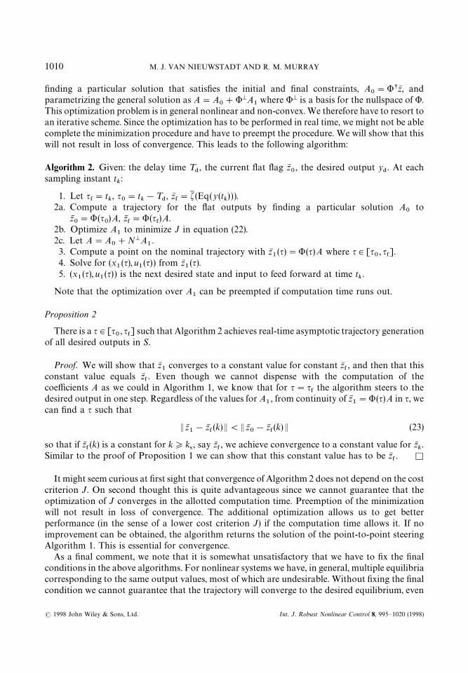
This optimization problem is in general nonlinear and non-convex. We therefore have to resort toan iterative scheme. Since the optimization has to be performed in real time, we might not be ablecomplete the minimization procedure and have to preempt the procedure. We will show that thiswill not result in loss of convergence. This leads to the following algorithm:

Algorithm 2. Given: the delay time ¹$, the current flat flag zN

0, the desired output y

$. At each

sampling instant tk:

1. Let q&"t

k, q

0"t

k!¹

$, zN

&"f1 (Eq(y(t

k) )).

2a. Compute a trajectory for the flat outputs by finding a particular solution A0

tozN0"'(q

0)A, zN

&"'(q

&)A.

2b. Optimize A1

to minimize J in equation (22).2c. Let A"A

0#NMA

1.

3. Compute a point on the nominal trajectory with zN1(q)"'(q)A where q3[q

0, q

&].

4. Solve for (x1(q), u

1(q)) from zN

1(q).

5. (x1(q), u

1(q)) is the next desired state and input to feed forward at time t

k.

Note that the optimization over A1

can be preempted if computation time runs out.

Proposition 2

There is a q3[q0, q

&] such that Algorithm 2 achieves real-time asymptotic trajectory generation

of all desired outputs in S.

Proof. We will show that zN1

converges to a constant value for constant zN&, and then that this

constant value equals zN&. Even though we cannot dispense with the computation of the

coefficients A as we could in Algorithm 1, we know that for q"q&the algorithm steers to the

desired output in one step. Regardless of the values for A1, from continuity of zN

1"'(q)A in q, we

can find a q such that

EzN1!zN

&(k)E(EzN

0!zN

&(k)E (23)

so that if zN&(k) is a constant for k*k

4, say zN

&, we achieve convergence to a constant value for zN

k.

Similar to the proof of Proposition 1 we can show that this constant value has to be zN&. K

It might seem curious at first sight that convergence of Algorithm 2 does not depend on the costcriterion J. On second thought this is quite advantageous since we cannot guarantee that theoptimization of J converges in the allotted computation time. Preemption of the minimizationwill not result in loss of convergence. The additional optimization allows us to get betterperformance (in the sense of a lower cost criterion J) if the computation time allows it. If noimprovement can be obtained, the algorithm returns the solution of the point-to-point steeringAlgorithm 1. This is essential for convergence.

As a final comment, we note that it is somewhat unsatisfactory that we have to fix the finalconditions in the above algorithms. For nonlinear systems we have, in general, multiple equilibriacorresponding to the same output values, most of which are undesirable. Without fixing the finalcondition we cannot guarantee that the trajectory will converge to the desired equilibrium, even



though we still get asymptotic tracking for signals in S. Indeed, simulations showed that thetrajectory might end up in an undesired equilibrium.

4. APPLICATION TO THE CALTECH DUCTED FAN

In this section we apply the real-time trajectory generation algorithms to the Caltech ducted fan,a thrust vectored, flight control experiment pictured in Figure 8.

The numerical computations in this section are done using the trajectory generation librarytglib, developed by M. van Nieuwstadt at Caltech. This library is available through anonymousftp from avalon.caltech.edu in the file /pub/vannieuw/software/trajgen.tar.gz. Thisfile contains the libraries, examples and documentation. The routines are in ANSI C and willcompile under different platforms. In particular, the simulations presented in this paper used thelibrary compiled on a UNIX platform, and the real-time experiments used the library compiledunder MS-DOS.

4.1. Simulations

We first simulate the real-time algorithms to study the role of the parameter ¹$and the tradeoff

between tracking and stability. For this study we have used a nonlinear model of the original

Figure 8. Photograph of the Caltech ducted fan experiment (courtesy of R. Bodenheimer)



Caltech ducted fan, described in detail in Reference 39. The main difference between this modeland the experiment shown in Figure 8 is that the stand dynamics are slightly more complicatedfor the original experiment and no wing was attached to the fan unit. The simulation model takesinto account the nonlinear stand dynamics, aerodynamic drag, inertial effects from the rotatingpropeller, and viscous friction. The flat model in equation (7) is used to generate the nominaltrajectories and only models the dynamics of the thrust and gravity.

We simulate the reference input as a file from which successive samples are read every sampleinstant. The reference trajectory is input to a trajectory generation module, whose output servesas a nominal trajectory. We wrap a simple static LQR controller around a nonlinear model of thefan. This controller was designed to stabilize hover. See Reference 39 for a detailed analysis ofseveral controller designs for this experiment. We assume we have knowledge of the full state. Onthe experiment this is achieved by differentiating and filtering the position signals.

First, we show how the ducted fan behaves without feedforward. The reference input is used togenerate an error signal to the controller. The reference input is a 1 m ramp in 3 s in thex direction at constant altitude. At each time instant we stabilize around the equilibrium pointgenerated by setting x and y equal to the reference input, and all other states equal to zero. This isthe conventional ‘one degree of freedom’ controller. Figure 9 shows that the trajectory followedby the fan lags far behind the desired trajectory.

In this plot and subsequent plots, the reference input is denoted by (xp,yp), the generateddesired trajectory (identical to the reference input in the one degree of freedom case) is denoted(xd,yd) and the variable name without a suffix denotes the real (experimental or simulated) timetrace of a quantity. The force parallel to the fan shroud is denoted ‘fpara’ the force perpendicularto the fan shroud is called ‘fperp’.

Figure 9. Ducted fan simulation: tracking with one-degree-of-freedom controller



Figure 10. Ducted fan simulation: tracking with algorithm 1, ¹$"60]¹

4"0)6 s

Next, we show for Algorithm 1 plots of the reference input, the generated trajectory, thesimulated trajectory for the (x, y) position of the fan, as well as the generated and simulatedtrajectory for h and the nominal forces.

Figure 10 shows these for a delay time ¹$"60 sampling periods of ¹

4"0)01 s. We see that the

fan follows the reference input much better than in the one-degree-of-freedom design. Clearly,there is an advantage in real-time trajectory generation. Figure 11 shows these for a delay time of¹$"100 sampling periods. It is clear that the larger delay results in better stability, i.e. lower

magnitude of h and the nominal forces, but poorer performance, since the delay is bigger.Figures 10 and 11 both show a large error in h right after the first and second peak of the

nominal h trace. We suspect this is caused by the inertia changing with altitude, which is not takeninto account in the nominal flat model, but is present in the simulation model. Note that theerrors occur simultaneously with a substantial error in altitude y.

Algorithm 2 was tested in simulation and the results are reported in References 34 and 40. Itbehaves as expected, in the sense that it penalizes the cost. The major problem is that theoptimization is a factor 10 too slow for realistic operator sampling rates. Improvement of thisoptimization is a subject of current research.

4.2. Hover-to-hover experiments

To demonstrate the viability of the two-degree-of-freedom approach, we first show somehover-to-hover transitions, both with one and two-degree-of-freedom controllers. Theseexperiments are performed on the Caltech ducted fan experiment. The ducted fan is mounted on



Figure 11. Ducted fan simulation: tracking with algorithm 1, ¹$"100]¹

4"1)0 s

a stand, as shown in Figure 12, and is controlled by an Intel 486,66 MHz PC. It uses a linearcurrent amplifier to regulate the current to the propeller, and PWM servos to steer the paddles. Ithas a NACA 0015 airofoil to generate lift, although for the experiments presented in this paper,the lift forces are negligible. Horizontal, vertical and pitch position are measured with encoders.Velocities are obtained by numerical differentiation and smoothing. Closed-loop control of theducted fan is accomplished using the Sparrow real-time kernel.43 Sparrow takes care of readingsensor input, writing actuator output, data logging, and necessary controller computations.

The dynamics of the ducted fan are essentially those given in Example 2, with additionalaerodynamic forces playing a role at high flight speeds. In the absence of these forces, the fandynamics are very close to the flat model. Therefore, for the hover-to-hover transitions consideredin this section, the flat model provides a good approximation to the actual dynamics of thesystem.

The computations in Section 3.2 were used to generate point-to-point motion of the system.The desired trajectory is a 4 m step in the positive x direction in 4 s. The one-degree-of-freedomcontroller uses a linear interpolation between initial and final state while keeping pitch zero. Thetwo-degree-of-freedom controller generates a non-zero nominal pitch trajectory. Figures 13 and14 show that the two-degree-of-freedom controller achieves considerable performance increase.The steady-state error in y is due to stiction in the stand.

4.3. Real-time trajectory generation experiments

Algorithm 1 was also implemented on the experimental apparatus, with the reference inputcomes from a joystick with two degrees of freedom. In order to obtain repeatable experiments, we



Figure 12. Ducted fan with stand

Figure 13. Ducted fan experiment: hover-to-hover transition for one-degree-of-freedom controller



Figure 14. Ducted fan experiment: hover-to-hover transition for two-degree-of-freedom controller

record the joystick input and read it back from a file for each trial (but without making use of theknowledge of future inputs). The joystick is interpreted as a commanded velocity signal, so thatthe reference trajectory for the (x, y) position is given by

x1(k)"f

x

k+i/0

gx(i) *¹

4

y1(k)"f

y

k+i/0

gy(i) *¹

4(24)

with gx,y

the joystick command in the (x, y) direction, respectively, and ( fx, f

y) some scaling

factors. We run the trajectory generation algorithm at 100 Hz, and the controller at 200 Hz. Thedelay time ¹

4"1)0 s, corresponding to 100 samples for the trajectory generation algorithms.

We conducted two experiments. The first one was the one-degree-of-freedom controller: thereference signal was used to generate an error signal in the output around which the fan wasstabilized. As in the simulations, the reference is denoted by (xp, yp), the desired trajectory by(xd,yd), and the measured position by (x, y). In the one-degree-of-freedom case (xp, yp)"(xd, yd).The results are depicted in Figure 15.

In the second experiment, we used the reference signal to generate a trajectory, as described inthis paper. The desired trajectory (xd,yd ) is generated by the trajectory generation module and isno longer equal to the reference input (xp, yp). The results are depicted in Figure 16. The real-timetrajectory generation algorithm gives a more aggressive response.



Figure 15. Ducted fan experiment: tracking with one-degree-of-freedom controller

Figure 16. Ducted fan experiment: tracking with real-time trajectory generation



5. SUMMARY

In this paper, we have proposed a formulation for the real-time trajectory generation problemwhich is compatible with a two-degree-of-freedom approach for tracking in motion controlalgorithms. We considered only the case of differentially flat systems, for which the trajectorygeneration problem can be formally reduced to an algebraic problem in terms of the flat outputsfor the system. By explicitly separating the tracking problem into a trajectory generation blockand a feedback compensation block, we are able to exploit the geometric structure of differentiallyflat systems without transforming the system into a single linear system. We thereby avoid someof the pitfalls commonly associated with feedback linearization and allow more freedom in thecontrol design.

We have described two algorithms for real-time trajectory generation for differentially flatsystems with unstable zero dynamics, and proved stability and convergence properties. The firstalgorithm generated a trajectory that steers from the current position to a desired final positiongiven by the reference input. We can trade-off stability versus performance by varying the delaytime. The second algorithm steers to a desired final position while minimizing a cost criterion,that typically limits the magnitude of the zero dynamics and/or the control inputs. The currentimplementation of the minimization is too slow for real-time implementation. Improving thisalgorithm is a subject of current research.

We have implemented the trajectory generation algorithms on a vectored thrust, flight controlexperiment constructed at Caltech. Experimental results show that the two-degree-of-freedomcontrollers perform much better than simpler linear controllers. For the experiments in thispaper, the fan was flown at low speeds. More aggressive trajectories have also been tested.34,44

Much work remains to be done on differentially flat systems, both from the theoreticalperspective and in the context of applications. At the present, constructive conditions for findingthe flat outputs of a mechanical system are not available except in a few special (i.e. lowdimensional) cases.45,46 In addition, for systems which are not differentially flat, it is likely thatapproximations can be used which will allow fast and efficient generation of approximatelyfeasible trajectories. Bounds on the sizes of the error in the performance of the system asa function of the degree of approximation will be needed in order to pursue efforts in thisdirection.

ACKNOWLEDGEMENTS

The authors would like to thank Mark Milam for his work on the ducted fan experiment.

REFERENCES

1. Shamma, J. S., ‘Robust stability with time-varying structured uncertainty’, IEEE ¹rans. Automat. Control, 39(4),714—724 (1994).

2. Packard, A., ‘Gain scheduling via linear fractional transformations’, Systems Control ¸ett., 22(2), 79—92 (1994).3. Hunt, L. R., R. Su and G. Meyer, ‘Global transformations of nonlinear systems’, IEEE ¹rans. Automat. Control,

AC-28(1), 24—31 (1983).4. Jakubczyk, B. and W. Respondek, ‘On linearization of control systems’, Bull. Acad. Polonaise des Sci. Ser. des Sci.

Math., XXVIII, 517—522 (1980).5. Isidori, A. and C. I. Byrnes, ‘Output regulation of nonlinear systems’, IEEE ¹rans. Automat. Control, 35(2), 131—140

(1990).6. Chen, D. G. and B. Paden, ‘Stable inversion of nonlinear nonminimum-phase systems’, Int. J. Control, 64(1), 81—97

(1996).



7. Devasia, S. and B. Paden, ‘Exact output tracking for nonlinear time-varying systems’, Proc. IEEE Control andDecision Conf., 1994, pp. 2346—2355.

8. Meyer, G., L. R. Hunt and R. Su, ‘Nonlinear system guidance’, Proc. IEEE Control and Decision Conf., 1995,pp. 590—595.

9. Getz, N. H. and K. Hedrick, ‘An internal equilibrium manifold method of tracking for nonlinear nonminimum phasesystems’, in Proc. IEEE Control and Decision Conf., 1995, pp. 2241—2245.

10. Getz, N. H., Dynamic inversion of nonlinear maps with applications to nonlinear control and robotics, Ph.D. thesis, UCBerkeley, Berkeley, California, 1995.

11. Fliess, M., J. Levine, Ph. Martin and P. Rouchon, ‘Sur les systemes non lineaires differentiellement plats’, C. R. Acad.Sci. Paris t. 315, Se& rie I, 619—624 (1992).

12. Fliess, M., J. Levine, Ph. Martin and P. Rouchon, ‘Linearisation par bouclage dynamique et transformations deLie-Backlund’, C. R. Acad. Sci. Paris t. 317, Se& rie I, 981—986 (1993).

13. Fliess, M., J. Levine, P. Martin and P. Rouchon, ‘Flatness and defect of non-linear systems: introductory theory andexamples’, Int. J. Control, 61(6), 1327—1361 (1995).

14. Fliess, M., J. Levine and P. Rouchon, ‘Generalized state variable representation for a simplified crane description’, Int.J. Control, 58(2), 277—283 (1993).

15. Rouchon, P., M. Fleiss, J. Levine and P. Martin, ‘Flatness, motion planning and trailer systems’, Proc. IEEE Controland Decision Conf., 1993, pp. 2700—2705.

16. Rouchon, P., M. Fliess, J. Levine and P. Martin, ‘Flatness and motion planning: the car with n trailers’, Proc.European Control Conf., 1992, pp. 1518—1522.

17. Martin, P., ‘Aircraft control using flatness’, in Multiconference on Computational Engineering in Systems Applications,pp. 194—199 (1996).

18. Martin, P., S. Devasia and B. Paden, ‘A different look at output tracking—Control of a VTOL aircraft’, Automatica,32(1), 101—107 (1994).

19. Chelouah, K., E. Delaleu, P. Martin and P. Rouchon, ‘Differential flatness and control of induction motors’,Multiconference on Computational Engineering in Systems Applications, 1996, pp. 80—85.

20. Martin, P. and P. Rouchon, ‘Flatness and sampling control of induction motors’, in ¼orkshop IFAC Symp., 1996.21. Levine, J., J. Lottin and J. C. Ponsart, ‘A nonlinear approach to the control of magnetic bearings’, IEEE ¹rans.

Control Systems ¹echnol., 5, 524—544 (1996).22. Rothfuss, R., J. Rudolph and M. Zeitz, ‘Flatness based control of a nonlinear chemical reactor model’, Automatica,

32(10), 1433—1439 (1996).23. Rouchon, P., ‘Vibrational control and flatness of chemical reactors’, in Multiconference on Computational Engineering

in Systems Applications, 1996, pp. 211—212.24. van Nieuwstadt, M., M. Rathinam and R. M. Murray, ‘Differential flatness and absolute equivalence’, Proc. IEEE

Control and Decision Conf., 1994, pp. 326—333. Also available as Caltech Technical Report CIT/CDS 94-006.25. Isidori, A., Nonlinear Control Systems, 2nd edn, Springer, Berlin, 1989.26. Nijmeijer, H. and A. van der Schaft, Nonlinear Dynamical Control Systems, Springer, Berlin, 1990.27. Cartan, E., Sur l’equivalence absolue de certains systemes d’equations differentielles et sur certaines familles de

courbes’, Guvres Comple% tes, Vol. II, Gauthier-Villars, 1953, pp. 1133—1168.28. Cartan, E., ‘Sur l’integration de certains systemes indetermines d’equations differentielles’, Guvres Comple% tes, Vol. II,

Gauthier-Villars, 1953, pp. 1169—1174.29. Sluis, W. M., Absolute Equivalence and its Applications to Control ¹heory. Ph.D. thesis, University of Waterloo,

Waterloo, Ontario, 1992.30. Charlet, B., J. Levine and R. Marino, ‘On dynamic feedback linearization’, Systems Control ¸ett., 13, 143—151

(1989).31. Fliess, M., Levine, J., P. Martin, F. Ollivier and P. Rouchen, ‘Flatness dynamic feedback linearizability: two

approaches’, Proc. European Control Conf., 1995.32. Martin, Ph., ‘Endogenous feedbacks and equivalence’, Mathematical ¹heory of Networks and Systems, Regensburg,

Germany, 1993.33. Bullo, F. and R. M. Murray, ‘Experimental comparison of trajectory trackers for a car with trailers’, IFAC ¼orld

Conf., 1996, pp. 407—412.34. van Nieuwstadt, M., ¹rajectory Generation for Nonlinear Control Systems. Ph.D. thesis, California Institute of

Technology, 1996.35. Martin, P. and P. Rouchon, ‘Feedback linearization and driftless systems’, Math. Control Signal Systems, 7, 235—254

(1994).36. Martin, P. and P. Rouchon, ‘Any (controllable) driftless system with 3 inputs and 5 states is flat’, Systems Control ¸ett.,

25, 167—173 (1995).37. Murray, R. M., ‘Trajectory generation for a towed cable system using differential flatness’, IFAC ¼orld Conf., 1996,

pp. 395—400.38. Murray, R. M., M. Rathinam and W. Sluis, ‘Differential flatness of mechanical control systems: a catalog of prototype

systems’, AsmeIMECE, San Francisco, 1995.



39. M. Kantner, B. Bodenheimer, P. Bendotti and R. M. Murray, ‘An experimental comparison of controllers fora vectored thrust, ducted fan engine’, Proc. American Control Conf., 1995, pp. 1956.

40. van Nieuwstadt, M. and R. M. Murray, ‘Approximate trajectory generation for differentially flat systems with zerodynamics’, Proc. IEEE Control and Decision Conf., 1995, pp. 4224—4230.

41. Grizzle, J. W., M. D. Di Benedetto and F. Lamnabhi-Lagarrigue, ‘Necessary conditions for asymptotic tracking innonlinear systems’, IEEE ¹rans. Automat. Control, 39(9), 1782—1795 (1994).

42. Khalil, H., Nonlinear Systems, Macmillan Publishing Company, New York, 1992.43. Murray, R. M., E. L. Wemhoff and K. Kantner, Sparrow 2.1 Reference Manual. California Institute of Technology,

1995. Available electronically from http://avalon.caltech.edu/&sparrow.44. van Nieuwstadt, M. and R. M. Murray, ‘Fast mode switching for a thrust vectored aircraft’, Multiconf. on

Computational Engineering in Systems Applications, Lille, France, 1996.45. Rathinam, M. and R. Murray, ‘Configuration flatness of lagrangian systems underactuated by one control’, Proc.

IEEE Control and Decision Conf., 1996, to appear.46. Rathinam, M. and R. Murray, ‘Flatness of nonlinear systems underactuated by two controls’, Proc. European Control

Conf., 1996, submitted.47. Martin, Ph., Contribution a% l’e& tude des syste%mes diffe& rentiellement plats, Ph.D. thesis, L’Ecole Nationale Superieure des

Mines de Paris, 1993.



real-time trajectory generation for differentially flat systems

Documents