real-time soil water dynamics using multisensor capacitance probes: laboratory calibration
TRANSCRIPT
Real-time Soil Water Dynamics Using Multisensor Capacitance Probes:Laboratory Calibration
I. C. Paltineanu and J. L. Starr*
ABSTRACTThere is a continued need for better methods to perform accurate,
real-time, nearly continuous soil water measurements at specific depthintervals, with minimal soil disturbance, and covering field-scale areas.The objectives of this research were to assess the characteristics of anewly developed multisensor capacitance probe and to calibrate thesensors against a Mattapex silt loam (fine-silty, mixed, mesic AquicHapludult) soil. The soil was uniformly packed in small increments,with the aid of a large hydraulic press, in a wooden box (35.5 by 35.5cm, 40.5 cm deep). Probe installation in the boxed soil mimicked thatrequired for correct field installation. A highly significant (r2 = 0.992for n = 15, and RMSE = 0.009 cm3 cm~3 water), nonlinear (0, =0.490 SF2-"74) relationship was found between the soil volumetric watercontent (0», cm3 cm 3) and the scaled frequency [SF = (Fa - F,)(F, -/\v)~']. The SF represents the ratio of individual sensor's frequency(inside PVC pipe) response in soil (Fs) compared with sensor re-sponses in air (/•',,) and in nonsaline water I/7,,) at room temperature(~ 22°C). Axial and radial sensitivity studies showed that these capaci-tance sensors give integrated readings over a primary depth intervalof 10 cm and a radial capacitance fringe within 10 cm of the wall ofthe access pipe. Temperature effects of air and water were measured,and the calculated effects on assessment of 0, were less than theRMSE for a temperature range of 10 to 30°C. Our calibration studiesindicate that these multisensor capacitance probes can be used toaccurately measure volumetric soil water contents in a soil watermonitoring system.
IN MOST AGRICULTURAL SOIL SYSTEMS, water contentsare highly dynamic in time — being affected by soil
USDA-ARS, Natural Resources Inst., Environmental ChemistryLab., Beltsville, MD 20705. Received 3 Oct. 1996. "Correspondingauthor ([email protected]).
Published in Soil Sci. Soc. Am. J. 61:1576-1585 (1997).
properties, soil and crop cultural practices, amounts andintensities of water inputs, and stage of crop growth. Theamount and status of water in soils, in turn, dramaticallyimpacts crop growth and the fate of agricultural chemi-cals applied to soils. The development of better manage-ment practices for efficient crop production and de-creasing deleterious impact on ground and surface waterquality requires greater understanding of the interde-pendent factors affecting the dynamics of water in soils.There is a continued need for better methods and tech-niques to perform accurate, real-time, nearly continuoussoil water measurement at specific depths, with minimalsoil disturbance, and covering field-scale areas with fewcables and a single data logger. Most of the well-knownsoil water monitoring methods present one or morelimitations to fulfilling the above requirements. A sur-vey of soil water measurement methods in current useshowed gravimetric analysis as the most commonmethod, followed by neutron thermalization, and, farbehind, time domain reflectometry (TDR) and gammaattenuation (Green and Topp, 1992).
The neutron thermalization method can be used tostudy spatial variability, e.g., with high spatial samplingintensity and with short time and depth interval readings(Paltineanu and Apostol, 1974). It has also been usedto study real-time temporal variability by using an auto-mated device that moved the neutron probe up anddown the access pipe at specific depth and time intervals(Marcesse and Couchat, 1974). However, high labor
Abbreviations: Fa, sensor frequency in air; Fs, sensor frequency in soil;FV, sensor frequency in water; RMSE, root mean square error; PVC,polyvinyl chloride; SF, scaled frequency; TDR, time domain reflec-tometry; CV, coefficient of variation; 6V, soil volumetric water content.
PALTINEANU & STARR: REAL-TIME SOIL WATER DYNAMICS USING CAPACITANCE PROBES 1577
costs and radioactive risk hazards and regulations, alongwith the neutron probe's individual and discrete datacollection, make the neutron thermalization method un-suitable for real-time soil water dynamics across largeareas.
Relationship of Dielectric Constantand Soil Water Content
More than 60 yr of international work have been spent onthe correlation between the apparent dielectric constant (K,)of the soil-air-water mixture and 6V at different electromag-netic field frequencies. Two methods that have been devel-oped in the last 20 yr are TDR and capacitance (Smith-Rose,1933; Chernyak, 1964; Thomas, 1966; Kuraz et al., 1970;Hoeskstra and Delaney, 1974; Wobschall, 1978; Topp et al.,1980; Dean et al, 1987; Hook et al., 1992; Whalley et al, 1992;Watson et al, 1995; Nadler and Lapid, 1996). Both methodsutilize the K.a of the soil surrounding the sensors in order tomeasure the 0V, which is an intrinsic characteristic of the soilwater-air mixture. At radio frequencies, the dielectric con-stant of pure water (Kv) at 20°C and atmospheric pressure is80.4, that of soil solids is 3 to 7, and that of air is 1. The #wis inversely related to temperature (Weast, 1980):
Kw = 78.54[l - 4.579 X 1(T3(?0 - 25)
+ 1.19 X lQ-5(t° - 25)2
- 2.8 X 10⁻⁸(f° - 25)''] [1]
that is approximately linear between O and 50°C, ranging from88.15 to 70.10, with a slope of approximately -4.5 X 10~3 °C~'.
The presence of salts in the soil water directly influencesthe dielectric behavior of soils, especially at frequencies <30MHz. Numerous experimental data for K, and 6V show a posi-tive and significant nonlinear correlation (Thomas, 1966; Toppet al, 1980; Zegelin et al, 1989; Timlin and Pachepsky, 1996).Experiments at frequencies >1 GHz showed that the nonline-arity can be attributed to the bound water, 6bw, which has atheoretical value of 4 or 1/20 that of free water (Wang andSchmugge, 1980; Wang, 1980). Due to the high forces actingon it, a bound water molecule interacts with the incident elec-tromagnetic wave in a manner dissimilar to that of a freewater molecule, thereby exhibiting a very different dielectricdispersion spectrum.
Electromagnetically, a soil medium can be represented asa four-component dielectric mixture of air, bulk soil, boundwater, and free water (Hallikainen et al, 1985). These re-searchers consider that the complex dielectric constants ofbound and free water are each functions of the electromag-netic frequency (F ), the temperature (T), and the salinity (S).Overall the K, at a given soil water content is a function ofmany factors including: (i) F, T, and S; (ii) 9V; (iii) the ratio6bw/6v, which is related to the soil surface area per unit volume;(iv) the bulk soil density (pb); (v) the shape of the soil particles;and (vi) the shape of the water inclusions. Dobson et al. (1985)developed a semiempirical mixing model that requires onlyeasily ascertained soil physical parameters such as 6V and tex-tural composition as inputs and that fits the measured dataat frequencies >4 GHz. Roth et al. (1990) successfully used thecomposite dielectric approach to measure soil water content,based on the fact that dielectric numbers of the air and solidphase are much less sensitive to temperature than that ofwater, and the influence of temperature on the dielectric num-ber of wet soil decreases with water content.
Time Domain Reflectometry MethodSince TDR and capacitance methods both measure soil K,
to obtain 6V, a brief review of the TDR method is of interest.The TDR method measures the velocity of propagation of ahigh-frequency signal reflected back from the end of a trans-mission line or wave guides in the soil. Wave guides (withtwo, three, or more rods) may be installed in the soil profilevertically or horizontally. Although vertical placement ofprobes may conduct heat into the soil via the metallic probesand possibly result in preferential flow of water along theprobes (Zegelin et al, 1992), the magnitude of the problem isnot well documented. Horizontal placement of probes requiresexcavation of a pit, which must then be backfilled to a condi-tion as close as possible to the soil's initial condition (Zegelinet al. (1992). The TDR method has been well documented byTopp et al. (1980) and Topp (1993). From laboratory experi-ments at frequencies from 1 MHz to 1 GHz, Topp et al. (1980)determined an empirical relationship between K, and 0V witha standard error of estimate of about 1.3% for all mineral soils.Their data agree very well with results of other researchersworking in frequency ranges of 20 MHz to 1 GHz and usinga wide range of soils and electrical techniques. A third-degreepolynomial relationship between K^ and 6V has been shownto be satisfactory for most mineral soils and conditions (Toppet al, 1980; Zegelin et al, 1992; Dalton, 1992; Topp, 1993).Nevertheless, soils with a high organic content, high 2:1 claycontent, or unusually high or low pb may require site-specificcalibrations (Herkelrath et al, 1991; Zegelin et al, 1992; Das-berg and Hopmans, 1992; Dirksen and Dasberg, 1993; Bridgeet al, 1996). Several of these studies also discuss the use ofTDR to estimate soil salinity, as can the capacitance technique(Watson et al, 1995), but the focus of our study is on soilwater content measurements.
Abundant experimental data show that the TDR techniqueis useful in studies of real-time soil water content dynamics(Topp et al, 1980,1982a,b; Topp and Davis, 1985; van Wesen-beeck and Kachanoski, 1988; Zegelin et al, 1989), with averageresolution commonly ranging from 0.02 to 0.005 cm3 cm~3.Special attention has been given to the spatial and temporaldistribution of soil water by designing different automatedTDR systems of data collection and monitoring techniques(van Wesenbeeck and Kachanoski, 1988; Baker and Allmaras,1990; Heimovaara and Bouten, 1990; Herkelrath et al, 1991).These systems often work quite well in small areas, but alimitation for measuring real-time soil water dynamics acrosslarge areas is the maximum cable length. Cables longer than=25 m increase the rise time of the voltage pulse due to thefiltering of the high-frequency components by the cable, whichresults in reflections with smaller amplitudes and smallerslopes (Heimovaara, 1993). Hook et al. (1992) proposed anew TDR technique that can extend the distance between theprobes and the TDR unit up to 100 m.
Capacitance MethodThe dielectric constant of soils can be measured by capaci-
tance. This method includes the soil as part of a capacitor, inwhich the permanent dipoles of water in the dielectric mediumare aligned by an electric field and become polarized. Tocontribute to the dielectric constant, the electric dipoles, ofany origin, must respond to the frequency of the electric field.The freedom of the dipoles to respond is determined by thelocal molecular binding forces so that the overall response isa function of molecular inertia, the binding forces, and thefrequency of the electric field (Dean et al, 1987). Measure-ment of the capacitance gives the dielectric constant, hence
1578 SOIL SCI. SOC. AM. J., VOL. 61, NOVEMBER-DECEMBER 1997
the water content of the soil. One of the first researchers toappreciate the need for using high frequency in the use ofcapacitance to measure K, was Thomas (1966). He measuredthe capacitance by a bridge method at 30 MHz, which requiredmanual balance, and a probe inserted directly into the surfacelayers of the soil (Dean et al., 1987). In a more straightforwardmethod for measuring capacitance, the capacitor is arrangedto be part of an oscillator circuit so that frequency of oscillationis a direct measure of the capacitance (Gardner et al., 1991).These researchers concluded that interference from acidityand salinity of soil water is reduced by operating at frequencieshigher than the minimum of 30 MHz, as soil conductivityeffects are inversely proportional to frequency. They alsoshowed that at 100 to 150 MHz these problems are sufficientlyreduced without encroaching into the very high frequenciesthat are operationally difficult for circuit technology. Duringthe last four decades, a few capacitance probes have beendesigned and manufactured, according to the respective devel-opments in electronics technologies. Portable capacitance
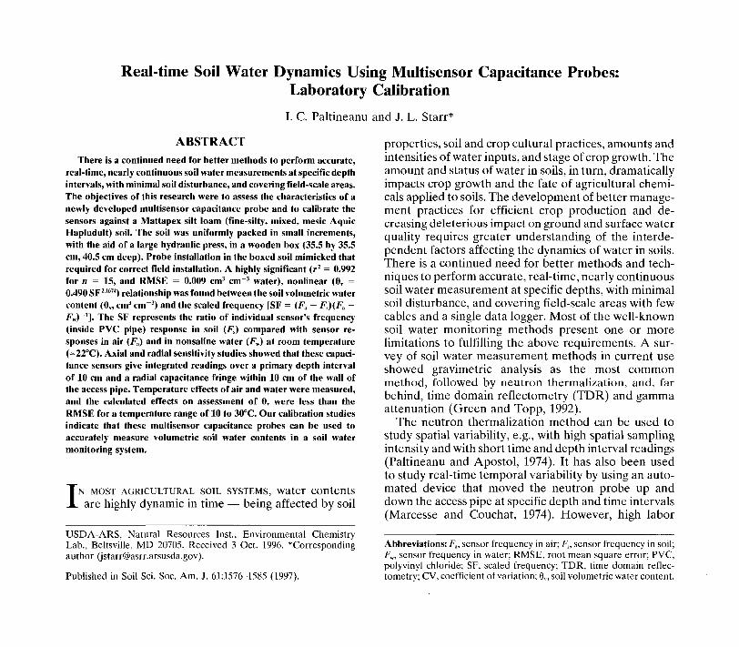
Fig. 1. Photo showing capacitance probe components: (1) plastic ex-trusion datum setting handle; (2) printed circuit board and 20-wayribbon cable; (3) capacitance sensors; (4) PVC access pipe; (5)removable cap with cable gland; (6) compression rubber ring; and(7) cutting edge.
probes using either direct contact between the capacitor ele-ments and soil (Chernyak, 1964; Thomas, 1966; Wobschall,1978; Whalley et al., 1992; Troxler Electronics Laboratories,1992; Nadler and Lapid, 1996) or probes manually inserted inPVC access tubes (Kuraz, 1982; Dean et al, 1987; TroxlerElectronics Laboratories, 1992) have been designed, cali-brated, and used in the field.
Field studies with a portable capacitance probe (ModelSENTRY 200AP1, Troxler Electronics Laboratories, Re-search Triangle Park, NC, patterned after Dean et al. [1987])have indicated that: the probe was unacceptable for soil watercontent measurements with fine sandy loam soil (Evett andSteiner, 1995); and changes in 6V are difficult to detect for dryor coarse-textured soils (Torner and Anderson, 1995). Thesefield studies, plus a few others, also compared results of thesame portable capacitance probe with different neutronprobes (Mead et al., 1994; Ley, 1994; Ayars et al, 1995).However, due to the difference in measurement method,spheres of influence, interference differences, etc., the twomethods will often give different measures and precisions.Thus, it seems inappropriate to consider the neutron probeas a standard for comparison for either the capacitance orTDR methods.
There are several problems with the use of portable capaci-tance probes that remain to be resolved. These problems in-clude: uncontrolled climate inside the PVC pipe, the influenceof positional changes in orientation within the access pipe,large and variable air gaps between the free-floating probeand PVC pipe, the extent of vertical axial sensitivity, nonuni-formity of the PVC pipe and thickness of its wall, and poorfield installation of the access pipe resulting in air gaps orchanges in pb along the pipe.
A new system for monitoring soil water content in real timehas been developed (EnviroSCAN, Sentek Pty Ltd., SouthAustralia) using semipermanent multisensor capacitanceprobes. The probes have been widely implemented in theirrigated agriculture industry of Australia since 1991 (Buss,1993), and have recently been introduced in the U.S. A waterand salinity measurement version of this equipment is underU.S. patent (Watson et al, 1995). These probes have designmodification that overcome the problems mentioned above.In addition, the system is designed so that they can be installedup to 500 m from the central data logger. The objective of thisresearch was to assess the characteristics of this multisensorcapacitance probe and to calibrate the capacitance sensorsunder laboratory conditions on a nonsaline silt loam soil.
MATERIALS AND METHODSMultisensor Capacitance Probe
The EnviroSCAN multisensor capacitance probe (Fig. 1)consists of a plastic extrusion (0.5-15 m or more), datumsetting handle, printed circuit board, and a 20-way ribboncable with connectors for capacitance sensors placed every0.1 m along its length. Each capacitance sensor consists of twobrass rings (50.5 mm o.d. and 25 mm high), mounted on aplastic sensor body separated by a 12-mm plastic ring (Fig.1). Plastic spring guides located on each end of the sensorkeep it in the center of the PVC access pipe, with a radial airgap of 0.4 mm between the sensor and the inside wall of thespecial-order PVC pipe. The conductive rings of the sensorform the plates of the capacitor. This capacitor is connectedto an LC oscillator, consisting of an inductor (L) and a capaci-
1 The mention of trade or manufacturer names is made for informa-tion only and does not imply an endorsement, recommendation, orexclusion by the USDA-ARS.
PALTINEANU & STARR: REAL-TIME SOIL WATER DYNAMICS USING CAPACITANCE PROBES 1579
tor (C) connected to circuitry that oscillates at a frequencydepending on the values of L and C. As the inductor is fixed(seven turns of 0.5-mm wire), the frequency of oscillationvaries depending on variations of capacitance. The oscillatingcapacitance field generated between the two rings of the sen-sor extends beyond the PVC access pipe into the surroundingmedium-soil (dielectric). The resonant frequency (F) can bemeasured using a general formula:
F = [2irV(LC)]- [2]where L is the circuit inductance and C is the total capacitance,which includes the soil components together with some con-stants (Chernyak, 1964; Kuraz et al, 1970; Kuraz, 1982;Wobschall, 1978; Dean et al, 1987; Gardner et al, 1991; Whal-ley et al, 1992; Evett and Steiner, 1995).
Since the area of the plates-rings and the distance betweenthe plates-rings are fixed on the sensor, the capacitance variesonly with varying complex dielectric constant of the materialsurrounding the plates-rings. These sensors have been de-signed to oscillate in excess of 100 MHz (inside access tubein free air) so as to be essentially immune to salinity andfertilizer effects at levels typically found in agricultural soils.The frequency of oscillation of the EnviroSCAN sensor isdivided by a factor of 2048, providing an output frequencyproportional to the frequency of oscillation. The data loggerpowers the sensor up for 0.5 s, then records the pulses during0.5 s to provide a count equal to half the output. For example,if the sensor is oscillating at 150 MHz, the output of the sensorswould be 73.242 kHz (1.5 X 10⁸/2048), so the logger wouldrecord a count of 36 621 (73 242/2). The data logger recordsthe output of the sensor by counting the pulses during a fixedtime (0.5 s), therefore the counts are proportional to the fre-quency of oscillation of the sensors.
The output (frequency) from the sensors primarily varieswith variations in the air/water ratio, and is measured by thedata logger at user-input sampling intervals to obtain a fre-quency in soil. Frequency readings of each sensor inside thePVC pipe, exposed to air and water (at room temperature,=22°C), are registered separately before installing the probein the soil. The frequencies in air, water, and soil are passedthrough a normalization equation to determine a normalizedor scaled frequency (SF), defined as:
SF = (Fa - Fs)(Fa - F,)-1 [3]where Fa is the frequency reading in the PVC access pipewhile suspended in air; Fs is the reading in the PVC accesspipe in soil; and Fw is the reading in the PVC access pipe inthe water bath. The SF has also been called a universal fre-
quency, but we prefer to use SF until a standard procedureis established and commonly recognized.
The data logger is capable of reading and storing data frommultiple sensors (£32 sensors in two to eight probes) and twoanalog channels at preselected sampling intervals ranging from1 to 9999 min. During the process of downloading data fromthe data logger, the SF is converted to 6V percentage usingeither a default or user-specified calibration equation. TheEnviroSCAN software can then display the information astotal water content in a profile (in millimeters) or at specificdepths (as a percentage). The graphs can then be interrogatedusing features such as zooming, scrolling, and panning. Thedownloaded data may also be converted to standard spread-sheet format for further analysis.
Soil and Soil PackingA Mattapex silt loam Ap horizon soil with about 35% sand,-
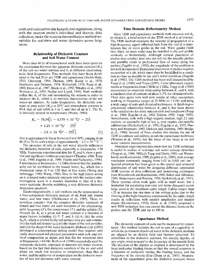
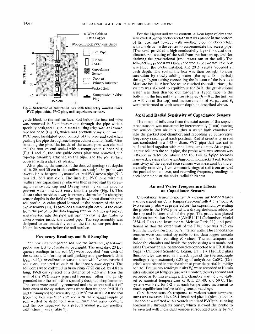
56% silt, 9% clay, and 0.08 g kg"1 organic C, was collectedfrom the USDA-ARS Beltsville Agricultural Research Cen-ter, Beltsville, MD. Soil from the O- to 20-cm depth wasbrought from the field to the greenhouse, spread out to par-tially dry, passed through a 6.35-mm sieve, and stored in large,covered plastic drums. This calibration study was conductedby packing soil in a plywood box (35.5 by 35.5 cm, by 40.5cm deep) with five repeated packings of soil with varyingpb (1.24-1.58 g cm"3) and 9V (0.07-0.37 cm3 cm"3) values asdescribed below and summarized in Table 1. A 7-cm-diam.hole was cut in the bottom of the box to accommodate installa-tion of the PVC access pipe. The box was constructed sothat we could simulate the manufacturer's requirements forinstallation of the capacitance probes in the field (Fig. 2).Fixed masses of soil were evenly spread inside the box by firstevenly spreading the soil on a tray with a sliding bottom plate.A 1.2-cm screen, suspended just above the bottom plate ofthe tray, allowed the plate to be drawn back to drop the soilevenly into the box. After checking the depth of the loosesoil (measured from the top of the box), and final leveling ofthe loose soil with a straightedge, the soil was then compressedby a 50-t hydraulic pump (Atlas Press Co, Kalamazoo, MI)to the predetermined soil thickness and wet bulk density (pt,w).The process was repeated in 1-cm compressed soil layers untilthe box was full of packed soil. Uniformity of packing waschecked by analysis of undisturbed soil cores as describedbelow. A box cover with an attached wooden block guide (15cm on each side, with a 6-cm-diam. guide hole cut throughthe center) for installing the PVC access pipe was securelyattached to the soil-filled box (Fig. 2). The PVC access pipe(described below) was installed by inserting it through the
Table 1. Measured soil physical characteristics (Mattapex silt loam) around the multisensor capacitance probe and corresponding scaledfrequency data.
Gravimetric water (8e) Wet bulk density (pbw) Dry bulk density (pb) Volumetric water (O,) Scaled frequency (SF)
10 cm 20 cm 30 cm 10 cm 20 cm 30 cm 10 cm 20 cm 30 cm 10 cm 20 cm 30 cm 10 cm 20 cm 30 cm
Pack 3: Avg.tCV(%)$
Pack 4: Avg.CV(%)
Pack 2: Avg.CV(%)
Pack 1: Avg.CV(%)
Pack 5: Avg.CV(%)
0.05840.90.10731.50.15440.70.16970.260.24570.4
kg kg '0.05840.90.10620.40.15300.20.16810.270.24742.8
0.05790.90.10710.80.15120.50.16660.40.25112.4
1.311.21.442.11.821.31.501.11.881.2
1.321.41.421.21.811.11.542.41.880.7
gci1.331.01.503.01.820.41.531.61.890.8
n ' ———1.241.21.312.01.581.41.281.11.511.2
1.241.31.291.21.571.01.312.51.511.1
1.261.31.352.91.580.51.321.51.511.2
0.07220.70.13981.60.23881.90.21730.90.37061.0
- m3 m 3 -0.07251.30.13671.40.23761.00.22092.40.37362.0
0.07291.40.14503.40.23780.50.22011.60.37901.3
0.3990.0410.5980.020.7280.0060.6970.0150.8830.016
0.3880.030.5460.0270.7220.0150.70.0110.8650.0093
0.3990.020.5520.0650.7200.02140.6960.00680.8880.0054
f Soil packing sequence. Average of five brass rings of 7.28-cm i.d. and 4.8-cm height placed around the sensors at - 2.5 mm from the PYC pipe wall.$ Coefficient of variation, n = 5.
1580 SOIL SCI. SOC. AM. J., VOL. 61, NOVEMBER-DECEMBER 1997
Wire Cable toData Logger
Wooden Block PVC Pipe Guide
CapacitanceSensor
i ~ " ~ Zone ofi (
---' Primary Influence——— Packed Soil
35.5 cmCompression RubberPlug
Fig. 2. Schematic of calibration box with temporary wooden blockPVC pipe guide, PVC pipe, and capacitance sensors.
guide block to the soil surface. Soil below the inserted pipewas removed in 5-cm increments through the pipe with aspecially designed auger. A metal cutting edge with an inwardtapered edge (Fig. 1), which was previously installed on thePVC pipe, facilitated good contact of the pipe and soil whenpushing the pipe through each augured increment of soil. Afterinstalling the pipe, the inside of the access pipe was cleanedand the bottom end sealed with a compression rubber plug(Fig. 1 and 2), the tube-guide cover plate was removed, thetop-cap assembly attached to the pipe, and the soil surfacecovered with a sheet of plastic.
After placing the sensors at the desired spacings (at depthsof 10, 20, and 30 cm in this calibration study), the probe wasinserted into the specially manufactured PVC access pipe (51.3mm i.d., 56.7 mm o.d.). The installed PVC pipe with themultisensor capacitance probe was then sealed shut by screw-ing a removable cap and O-ring assembly on the pipe toprevent water and dust entry into the probe (Fig. 1). Thisclosure also provides a way to remove the probe for changingsensor depths in the field or for repairs without disturbing thesoil profile. A cable gland located at the bottom of the top-cap assembly (Fig. 1) provides a water-tight entry of the cablefrom the probe to the data logging station. A silica gel packetwas inserted into the pipe just prior to closing the probe toabsorb water inside the closed pipe. The cap assembly wasdesigned to automatically center the first sensor position at10-cm increments below the soil surface.
Frequency Readings and Soil SamplingThe box with compacted soil and the installed capacitance
probe was left to equilibrate overnight. The next day, 20 fre-quency readings in the soil (Fs) were recorded from each ofthe sensors. Uniformity of soil packing and gravimetric data(pbw, and 6g) for calibration was obtained with five undisturbedsoil cores, centered at each of the three sensor depths. Thesoil cores were collected in brass rings (7.28 cm i.d. by 4.8 cmlong, 199.8 cm3) placed at a distance of =2.5 mm from thewall of the PVC access pipe and from each other, and gentlypounded into the soil with a specially designed drop hammer.The cores were carefully removed and the excess soil cut offboth ends of the cylinders; cores were then weighed (±0.01 g)and subsampled for oven drying (105°C for 48 h). All the soilfrom the box was then remixed with the original supply ofsoil, wetted or dried to a new uniform soil water content,and the box repacked to a predetermined pbw for anothercalibration point (Table 1).
For the highest soil water content, a 3-cm layer of dry sandwas leveled on top of cheesecloth that was placed in the bottomof the box, and covered with another piece of cheeseclothwith a hole cut in the center to accommodate the access pipe.(The sand provided a high-conductivity layer for quasi one-dimensional wetting of the soil from the bottom up, and fordraining the gravitational [free] water out of the soil.) Thesoil-packing process was then repeated as before until the boxwas filled, the probe installed, and 20 Fs values recorded ateach depth. The soil in the box was then brought to nearsaturation by slowly adding water (during a 48-h period)through Tygon tubing connecting the bottom of the box to aMariotte bottle. After free water reached the soil surface, thesystem was allowed to equilibrate for 24 h, the gravitationalwater was then drained out through a Tygon tube in thebottom of the box until the flow stopped (h = O at the bottomto —40 cm at the top) and measurements of Fs, pbw, and 6gwere performed at each sensor depth as described above.
Axial and Radial Sensitivity of Capacitance SensorsThe range of influence from the axial center of the capaci-
tance sensors was measured by incrementally (1 cm) movingthe sensors from air into either a water bath chamber orinto the packed soil chamber, and recording 20 consecutivefrequency readings at each position. Radial sensitivity in soilwas conducted in a 0.42-m-diam. PVC pipe that was cut inhalf and held together with metal circular clamps. After pack-ing the soil into the split pipe, the probe with two sensors wasinstalled as described above and the two half-pipe sectionsremoved, leaving a free-standing column of packed soil. Radialsensitivity of the capacitance sensors was measured by incre-mentally removing 1-cm concentric rings of soil from aroundthe packed soil column, and recording frequency readings ateach increment of the soil's radial thickness.
Air and Water Temperature Effectson Capacitance Sensors
Capacitance sensor response to various air temperatureswas measured inside a temperature-controlled chamber. Atwo-sensor probe was prepared for this experiment by sealingthe probe in the PVC pipe with a drying desiccant added tothe top and bottom ends of the pipe. The probe was placedinside an incubation chamber (AMBI-HI-LO chamber, Model3554-35, Lab Line Instruments, Melrose Park, IL), and posi-tioned so that the outer wall of the PVC pipe was >25 cmfrom the incubation chamber's interior walls. The capacitancesensors were connected by cable to the data logger outsidethe chamber for recording F.t values. The air temperatureinside the chamber and inside the probe casing was monitoredusing Cu-constantan thermocouples connected to a CR10 datalogger (Campbell Scientific, Logan, UT). (A Hg-filled glassthermometer was used as a check against the thermocouplereadings.) Approximately 0.25 kg of anhydrous CaSO4 (Dri-erite) were placed in the chamber to provide partial humiditycontrol. Frequency readings in air (Fa) were recorded at 10-minintervals, and air temperature was monitored every second andrecorded as 10-min averages. The chamber was incrementallyset to nominal temperatures of O, 5, 20, 40, and 50°C. Thesystem was held for >2 h at each temperature increment toreach equilibrium before taking sensor readings.
Capacitance sensor's response to various water tempera-tures was measured in a 26-L insulated plastic (picnic) cooler.The cooler was fitted with a Sentek standard PVC pipe runninghorizontally through its center, which allowed the probe tobe inserted with individual sensors surrounded axially by >7
PALTINEANU & STARR: REAL-TIME SOIL WATER DYNAMICS USING CAPACITANCE PROBES 1581
cm and radially by >10 cm of water. Frequency readings inwater (Fw) were recorded for a temperature range of 8 to54°C. The temperature of the water inside the cooler wasmonitored using two Cu-constantan thermocouples, placed =5cm from the inside wall at each end of the cooler, connectedto a CR10 data logger (Campbell Scientific). (A Hg-filled glassthermometer was again used for comparison to the thermo-couple readings.) Uniform temperature throughout the coolerwas obtained with a pump that recirculated water from oneend of the cooler to the other end. The water temperaturewas controlled by replacing a volume of water with iced orhot tap water.
RESULTS AND DISCUSSIONUniformity of Soil Packing
Soil physical characteristics associated with each soilpacking and water content were obtained from five un-disturbed cores taken at 2.5-mm distance from the PVCpipe (Table 1). The soil packing procedures resulted inlow spatial variability of the measured parameters, withCVs (n = 5) ranging from 0.5 to 2.9% for pb, 0.2 to2.8% for 6g, 0.5 to 3.4% for 9V, and 0.0054% to 0.065%for SF. These data indicate that the precision of calibra-tion is primarily limited by the errors associated withobtaining accurate gravimetric measurements. Thus, aswith other in situ instruments for soil water measure-ments, accurate laboratory or field calibration of capaci-tance sensors requires carefully obtained soil physicalcharacteristics from the primary zone of influence ofthe sensor.
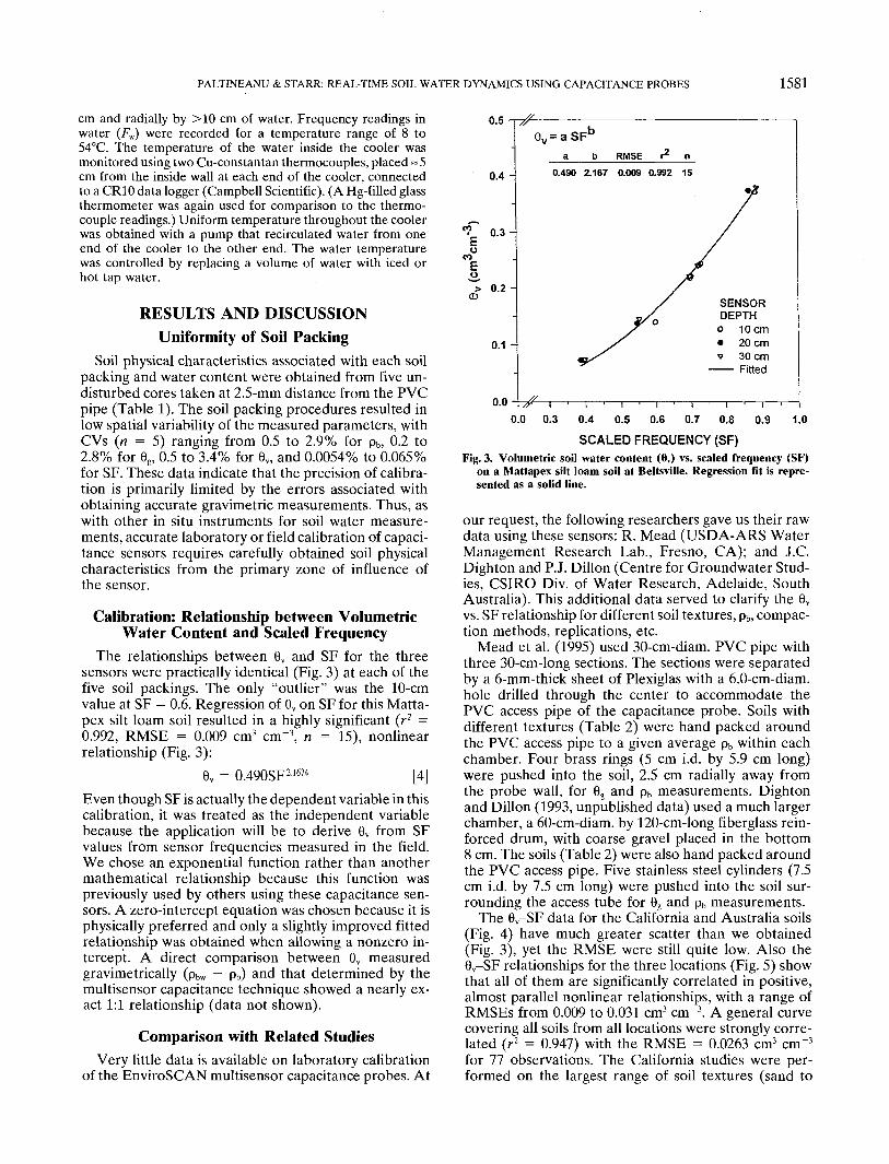
Calibration: Relationship between VolumetricWater Content and Scaled Frequency
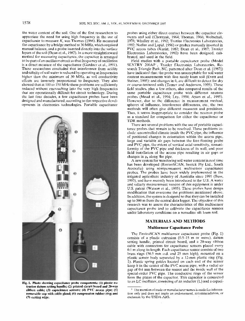
The relationships between 0V and SF for the threesensors were practically identical (Fig. 3) at each of thefive soil packings. The only "outlier" was the 10-cmvalue at SF = 0.6. Regression of 0V on SF for this Matta-pex silt loam soil resulted in a highly significant (r2 =0.992, RMSE = 0.009 cm3 cm'3, n = 15), nonlinearrelationship (Fig. 3):
6V = 0.490SF21674 [4]Even though SF is actually the dependent variable in thiscalibration, it was treated as the independent variablebecause the application will be to derive 6V from SFvalues from sensor frequencies measured in the field.We chose an exponential function rather than anothermathematical relationship because this function waspreviously used by others using these capacitance sen-sors. A zero-intercept equation was chosen because it isphysically preferred and only a slightly improved fittedrelationship was obtained when allowing a nonzero in-tercept. A direct comparison between 9V measuredgravimetrically (pbw - pb) and that determined by themultisensor capacitance technique showed a nearly ex-act 1:1 relationship (data not shown).
Comparison with Related StudiesVery little data is available on laboratory calibration
of the EnviroSCAN multisensor capacitance probes. At
0.5
0.4-
0.3 -
0.2 -
0.1 -
0.0
ev=aSFL
RMSE n0.490 2.167 0.009 0.992 15
0.0 0.3 0.4 0.5 0.6 0.7 0.8 0.9 1.0
SCALED FREQUENCY (SF)Fig. 3. Volumetric soil water content (Ov) vs. scaled frequency (SF)
on a Mattapex silt loam soil at Beltsville. Regression fit is repre-sented as a solid line.
our request, the following researchers gave us their rawdata using these sensors: R. Mead (USDA-ARS WaterManagement Research Lab., Fresno, CA); and J.C.Dighton and P.J. Dillon (Centre for Groundwater Stud-ies, CSIRO Div. of Water Research, Adelaide, SouthAustralia). This additional data served to clarify the Ovvs. SF relationship for different soil textures, pb, compac-tion methods, replications, etc.
Mead et al. (1995) used 30-cm-diam. PVC pipe withthree 30-cm-long sections. The sections were separatedby a 6-mm-thick sheet of Plexiglas with a 6.0-cm-diam.hole drilled through the center to accommodate thePVC access pipe of the capacitance probe. Soils withdifferent textures (Table 2) were hand packed aroundthe PVC access pipe to a given average pb within eachchamber. Four brass rings (5 cm i.d. by 5.9 cm long)were pushed into the soil, 2.5 cm radially away fromthe probe wall, for 6g and pb measurements. Dightonand Dillon (1993, unpublished data) used a much largerchamber, a 60-cm-diam. by 120-cm-long fiberglass rein-forced drum, with coarse gravel placed in the bottom8 cm. The soils (Table 2) were also hand packed aroundthe PVC access pipe. Five stainless steel cylinders (7.5cm i.d. by 7.5 cm long) were pushed into the soil sur-rounding the access tube for 0g and pb measurements.
The 0V-SF data for the California and Australia soils(Fig. 4) have much greater scatter than we obtained(Fig. 3), yet the RMSE were still quite low. Also the0V-SF relationships for the three locations (Fig. 5) showthat all of them are significantly correlated in positive,almost parallel nonlinear relationships, with a range ofRMSEs from 0.009 to 0.031 cm3 cm~3. A general curvecovering all soils from all locations were strongly corre-lated (r2 = 0.947) with the RMSE = 0.0263 cm3 cm"3
for 77 observations. The California studies were per-formed on the largest range of soil textures (sand to
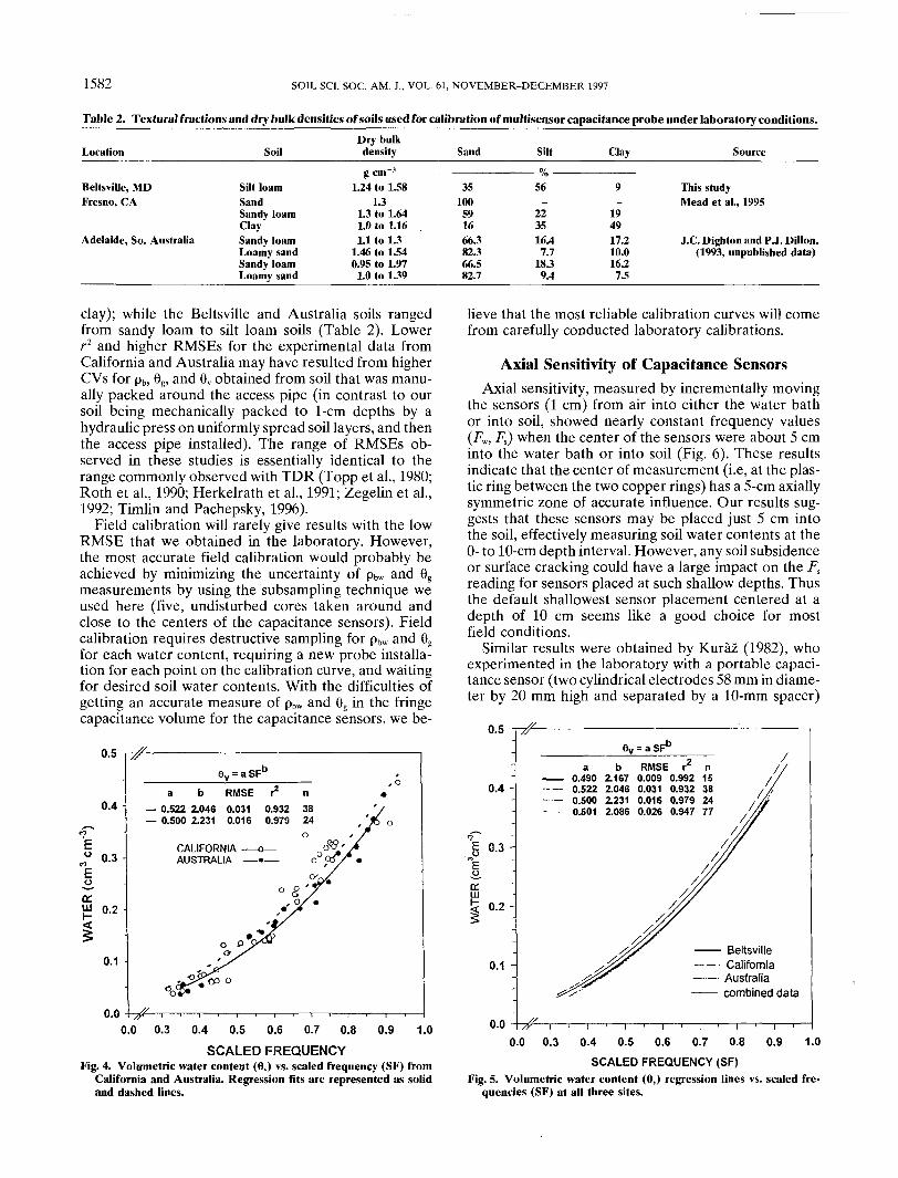
1582 SOIL SCI. SOC. AM. J., VOL. 61, NOVEMBER-DECEMBER 1997
Table 2. Textural fractions and dry bulk densities of soils used for calibration of niultisensor capacitance probe under laboratory conditions.
Location
Beltsville, MDFresno, CA
Adelaide, So. Australia
Soil
Silt loamSandSandy loamClaySandy loamLoamy sandSandy loamLoamy sand
Dry bulkdensity
gem 3
1.24 to 1.581.3
1.3 to 1.641.0 to 1.161.1 to 1.3
1.46 to 1.540.95 to 1.971.0 to 1.39
Sand
35100591666.382.366.582.7
SiltO/———— /o —————
56_
223516.47.7
18.39.4
Clay
9_
194917.210.016.27.5
Source
This studyMead et al., 1995
J.C. Dighton and P.J. Dillon,(1993, unpublished data)
clay); while the Beltsville and Australia soils rangedfrom sandy loam to silt loam soils (Table 2). Lowerr2 and higher RMSEs for the experimental data fromCalifornia and Australia may have resulted from higherCVs for pb, 6g, and 9V obtained from soil that was manu-ally packed around the access pipe (in contrast to oursoil being mechanically packed to 1-cm depths by ahydraulic press on uniformly spread soil layers, and thenthe access pipe installed). The range of RMSEs ob-served in these studies is essentially identical to therange commonly observed with TDK (Topp et al., 1980;Roth et al., 1990; Herkelrath et al., 1991; Zegelin et al,1992; Timlin and Pachepsky, 1996).
Field calibration will rarely give results with the lowRMSE that we obtained in the laboratory. However,the most accurate field calibration would probably beachieved by minimizing the uncertainty of pbw and 6gmeasurements by using the subsampling technique weused here (five, undisturbed cores taken around andclose to the centers of the capacitance sensors). Fieldcalibration requires destructive sampling for pbw and 6gfor each water content, requiring a new probe installa-tion for each point on the calibration curve, and waitingfor desired soil water contents. With the difficulties ofgetting an accurate measure of pbw and 6g in the fringecapacitance volume for the capacitance sensors, we be-
0.5
0.4
u
OLUJ
I
0.3 -
0.2
0.1
0.0
ev = a SF"a b RMSE r2 n
~ 0.522 2.046 0.031 0.932 38— 0.500 2.231 0.016 0.979 24
CALIFORNIA ——o—AUSTRALIA ——•——
0.0 0.3 0.4 0.5 0.6 0.7 0.8 0.9 1.0
SCALED FREQUENCYFig. 4. Volumetric water content (6,) vs. scaled frequency (SF) from
California and Australia. Regression fits are represented as solidand dashed lines.
lieve that the most reliable calibration curves will comefrom carefully conducted laboratory calibrations.
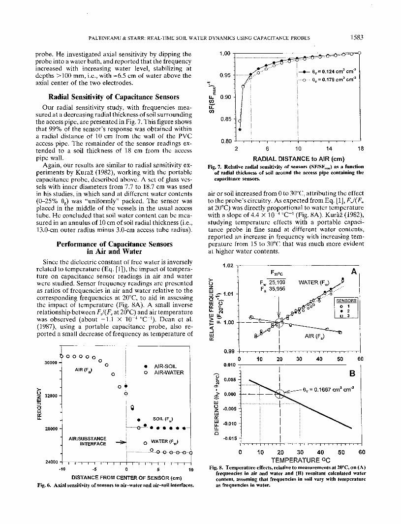
Axial Sensitivity of Capacitance SensorsAxial sensitivity, measured by incrementally moving
the sensors (1 cm) from air into either the water bathor into soil, showed nearly constant frequency values(Fm Fs) when the center of the sensors were about 5 cminto the water bath or into soil (Fig. 6). These resultsindicate that the center of measurement (i.e, at the plas-tic ring between the two copper rings) has a 5-cm axiallysymmetric zone of accurate influence. Our results sug-gests that these sensors may be placed just 5 cm intothe soil, effectively measuring soil water contents at theO- to 10-cm depth interval. However, any soil subsidenceor surface cracking could have a large impact on the Fsreading for sensors placed at such shallow depths. Thusthe default shallowest sensor placement centered at adepth of 10 cm seems like a good choice for mostfield conditions.
Similar results were obtained by Kuraz (1982), whoexperimented in the laboratory with a portable capaci-tance sensor (two cylindrical electrodes 58 mm in diame-ter by 20 mm high and separated by a 10-mm spacer)
0.5
0.4 -
E 0.3
0.1 -
6V = a SF"
a b RMSE r2 n0.490 2.167 0.009 0.992 150.522 2.046 0.031 0.932 380.500 Z231 0.016 0.979 240.501 2.086 0.026 0.947 77
— — • California—— Australia—— combined data
0.00.0 0.3 0.4 0.5 0.6 0.7 0.8 0.9 1.0
SCALED FREQUENCY (SF)Fig. 5. Volumetric water content (6V) regression lines vs. scaled fre-
quencies (SF) at all three sites.
PALTINEANU & STARR: REAL-TIME SOIL WATER DYNAMICS USING CAPACITANCE PROBES 1583
probe. He investigated axial sensitivity by dipping theprobe into a water bath, and reported that the frequencyincreased with increasing water level, stabilizing atdepths >100 mm, i.e., with =6.5 cm of water above theaxial center of the two electrodes.
Radial Sensitivity of Capacitance SensorsOur radial sensitivity study, with frequencies mea-
sured at a decreasing radial thickness of soil surroundingthe access pipe, are presented in Fig. 7. This figure showsthat 99% of the sensor's response was obtained withina radial distance of 10 cm from the wall of the PVCaccess pipe. The remainder of the sensor readings ex-tended to a soil thickness of 18 cm from the accesspipe wall.
Again, our results are similar to radial sensitivity ex-periments by Kuraz (1982), working with the portablecapacitance probe, described above. A set of glass ves-sels with inner diameters from 7.7 to 18.7 cm was usedin his studies, in which sand at different water contents(0-25% 6g) was "uniformly" packed. The sensor wasplaced in the middle of the vessels in the usual accesstube. He concluded that soil water content can be mea-sured in an annulus of 10 cm of soil radial thickness (i.e.,13.0-cm outer radius minus 3.0-cm access tube radius).
Performance of Capacitance Sensorsin Air and Water
Since the dielectric constant of free water is inverselyrelated to temperature (Eq. [1]), the impact of tempera-ture on capacitance sensor readings in air and waterwere studied. Sensor frequency readings are presentedas ratios of frequencies in air and water relative to thecorresponding frequencies at 20°C, to aid in assessingthe impact of temperature (Fig. 8A). A small inverserelationship between FJ(Fa at 20°C) and air temperaturewas observed (about -1.1 X 10~4 °C~'). Dean et al.(1987), using a portable capacitance probe, also re-ported a small decrease of frequency as temperature of
b o o o o o36000 -
Z111O
32000 -
28000 -
AIR (FJ • AIR-SOILO AIR-WATER
~o~
AIR:SUBSTANCEINTERFACE
24000 • —i—i—i—i—i—i—i—i—i—i—i—i—i
SOIL(FS)
0 WATER (Fw)
Q o o o o o <J>I—I—I—I—
-10 -5 O 5 10
DISTANCE FROM CENTER OF SENSOR (cm)Fig. 6. Axial sensitivity of sensors to air-water and air-soil interfaces.
1.00
0.95 -
U- 0.90 -\V)
0.85
0.8010 14 18
RADIAL DISTANCE to AIR (cm)Fig. 7. Relative radial sensitivity of sensors (SF/SFmax) as a function
of radial thickness of soil around the access pipe containing thecapacitance sensors.
air or soil increased from O to 30°C, attributing the effectto the probe's circuitry. As expected from Eq. [1], FJ(FVIat 20°C) was directly proportional to water temperaturewith a slope of 4.4 X 10~4 "CT1 (Fig. 8A). Kuraz (1982),studying temperature effects with a portable capaci-tance probe in fine sand at different water contents,reported an increase in frequency with increasing tem-perature from 15 to 30°C that was much more evidentat higher water contents.
1.02
g
1-1.01a^~LU QK °1"- °u tp u-1.00_̂iLUo:
0.99
r20°C
AIR (Fa)
10 20 30 40 50 600.010
LU
LU
0.005 -
-0.005
-0.010 -
-0.015 -
B
= 0.1667 cm3 crrf3
10 50 6020 30 40TEMPERATURE °c
Fig. 8. Temperature effects, relative to measurements at 20°C, on (A)frequencies in air and water and (B) resultant calculated watercontent, assuming that frequencies in soil vary with temperatureas frequencies in water.
1584 SOIL SCI. SOC. AM. J., VOL. 61, NOVEMBER-DECEMBER 1997
The calculated 6V resulting from simultaneouslychanging air, water, and soil temperature was estimatedby: (i) assuming that the temperature effect on Fs wasthe same as for Fw, i.e., same slope; (ii) for a specificexperimental Fs value at 20°C (6V = 0.1667), the slopeof Fw °C~1 was applied and different values of Fs ob-tained; (iii) generating a table of Fa, Fm Fs, and thecorresponding SF values for a temperature range of 5to 55°C; and (iv) calculating the water content from thecalibrated 6V vs. SF relationship (Eq. [4]). The fractionalvolumetric water contents were then all normalized to20°C by difference (Fig. 8B). The apparent "error" dueto temperature effects across the temperature range of10 to 30°C was in the order of the RMSE for our calibra-tion curve (0.007 cm3 cnr3 vs. RMSE of 0.009 cm3 cm-3).The calculated effects of temperature on 0V is only afirst approximation, but may not be too far off sincethe KZ of the soil-air-water mixture will be dominatedby the Km except at low water contents.
Stability of sensors with time was measured in air at= 11.0°C in the incubation chamber in which the airtemperature decreased very slowly (0.0076°C d~'),showing slowly increasing Fa with time. During the 3-dperiod, 432 pairs of temperature-Fa readings (every 10min) showed a CV of external temperature of 0.768%while the CV for Fa was more than two orders of magni-tude smaller, or 0.0042% (1.5 out of 36000). The slightvariation of the frequency readings we and others (Meadet al., 1996) observed in the air and water should consti-tute an object of further research. Variations in soil andwater temperature may correlate with the movementof water vapors under conditions of temperature inver-sions (Bunnenberg and Kuhn, 1974). Clearly, more re-search is needed to clarify the impact of changing tem-perature on capacitance sensor output. However, theseexperiments and analysis suggest that the effects arenegligible unless the soil temperature is significantlyoutside the range of 10 to 30°C.
CONCLUSIONSOur laboratory calibration studies, performed in the
carefully packed silt loam soil, indicate that this multi-sensor capacitance probe can be used to fulfill the needfor a soil water monitoring system that can performaccurate soil water measurements at narrow depth inter-vals with minimal soil disturbance. This conclusion isbased on the following observations:
1. A nonlinear relationship between 6V and scaledsensor frequencies (SF) was found using this capacitancetechnique (9V = 0.490SF21674) that is highly significantand has a low standard error (r2 = 0.992, n = 5, andRMSE = 0.009 cm3 cnr3).
2. Close agreement of 0V vs. SF was found betweenlaboratory calibration data (loamy sand to silt loamsoils) from Australia and Beltsville. Even with the mostdivergent laboratory calibration data from California(sand to clay soil), the shapes of all the curves wereessentially the same with low standard errors.
3. Axial and radial sensitivity studies showed that
these capacitance sensors gave integrated readingswithin a primary depth interval of 10 cm, and a primaryradial capacitance fringe measurement within 10 cm ofthe wall of the access pipe.
4. The sensors were tested in air and water for a widetemperature range with small linear but opposite effectson the air and water frequencies. Errors associated withfrequency readings at simulated soil temperatures from10 to 30°C were calculated to be less than the RMSEfor our calibration curve.
With the known difficulties of getting accurate mea-surements of pbw and 0g in the fringe capacitance volumearound the capacitance sensors under field conditions,the most reliable relationship between 6V and sensorfrequencies in soil will most likely result from carefullyconducted laboratory calibrations.
More calibration research with these capacitance sen-sors is needed (as has been the case with all methodsthat use Ka to calculate soil water content) for specialsoils (e.g., swelling 2:1 clays or high organic matter con-tent) and for extremes of soil temperature that can occurdiurnally with bare surface soils and seasonally inmany climates.
ACKNOWLEDGMENTS
We wish to thank Mr. Peter Downey, technician at USDA-ARS BARC NRI-ECL, Beltsville, MD; Ms. Kristin Measellsand Ms. Catherine Wells, graduate students of the Universityof Maryland at College Park for their assistance. We alsoexpress our appreciation to Mr. R.M. Mead, USDA-ARS,Fresno, CA; Dr. J.C. Dighton and Dr. P.J. Dillon, CSIRO,Glen Osmond, South Australia, for sharing their raw calibra-tion data; and Mr. P. Buss, Sentek Pty Ltd, Kent Town, SouthAustralia, for his assistance and technical support.
PALTINEANU & STARR: REAL-TIME SOIL WATER DYNAMICS USING CAPACITANCE PROBES 1585