UNIVERSIDADE DE LISBOAFACULDADE DE CIÊNCIAS

DEPARTAMENTO DE INFORMÁTICA

Real-Time Scheduling in MulticoreTime- and Space-Partitioned Architectures

João Pedro Gonçalves Crespo Craveiro

DOUTORAMENTO EM INFORMÁTICAESPECIALIDADE ENGENHARIA INFORMÁTICA

2013

UNIVERSIDADE DE LISBOAFACULDADE DE CIÊNCIAS

DEPARTAMENTO DE INFORMÁTICA

Real-Time Scheduling in MulticoreTime- and Space-Partitioned Architectures

João Pedro Gonçalves Crespo Craveiro

Tese orientada pelo Prof. Doutor José Manuel de Sousa de Matos Rufino,especialmente elaborada para a obtenção do grau de DOUTOR emINFORMÁTICA, especialidade ENGENHARIA INFORMÁTICA

2013

This work was partially supported by

the European Space Agency Innovation (ESA) Triangle Initiative programthrough ESTEC Contract 21217/07/NL/CB, Project AIR-II

·

the European Commission Seventh Framework Programme (FP7)through project KARYON (IST-FP7-STREP-288195)

·

Fundação para a Ciência e a Tecnologia (FCT), with Égide/CAMPUSFRANCEthrough the PESSOA programme transnational cooperation project SAPIENT

·

Fundação para a Ciência e a Tecnologia (FCT)through multiannual funding to the LaSIGE research unit, the CMU|Portugal programme,

the Individual Doctoral Grant to the author (SFRH/BD/60193/2009), and

project READAPT (PTDC/EEI-SCR/3200/2012)

Abstract

The evolution of computing systems to address size, weight and powerconsumption (SWaP) has led to the trend of integrating functions (oth-erwise provided by separate systems) as subsystems of a single system.To cope with the added complexity of developing and validating sucha system, these functions are maintained and analyzed as componentswith clear boundaries and interfaces. In the case of real-time systems,the adopted component-based approach should maintain the timelinessproperties of the function inside each individual component, regardlessof the remaining components. One approach to this issue is time andspace partitioning (TSP)—enforcing strict separation between compo-nents in the time and space domains. This allows heterogeneous compo-nents (different real-time requirements, criticality, developed by differentteams and/or with different technologies) to safely coexist. The con-cepts of TSP have been adopted in the civil aviation, aerospace, and (tosome extent) automotive industries. These industries are also embracingmultiprocessor (or multicore) platforms, either with identical or non-identical processors, but are not taking full advantage thereof becauseof a lack of support in terms of verification and certification. Further-more, due to the use of the TSP in those domains, compatibility betweenTSP and multiprocessor is highly desired. This is not the present case,as the reference TSP-related specifications in the aforementioned indus-tries show limited support to multiprocessor. In this dissertation, wedefend that the active exploitation of multiple (possibly non-identical)processor cores can augment the processing capacity of the time- andspace-partitioned (TSP) systems, while maintaining a compromise withsize, weight and power consumption (SWaP), and open room for sup-porting self-adaptive behavior. To allow applying our results to a moregeneral class of systems, we analyze TSP systems as a special case of hi-erarchical scheduling and adopt a compositional analysis methodology.

ResumoA evolução dos sistemas computacionais para endereçar questões de ta-manho, peso e consumo energético conduziu à tendência de integrar fun-ções (de outra forma fornecidas por sistemas separados) como subsiste-mas de um único sistema. Para lidar com a complexidade do desenvolvi-mento e validação de tal sistema, estas funções são mantidas e analisadascomo componentes com fronteiras e interfaces bem definidos. No casodos sistemas de tempo-real, a abordagem baseada em componentes ado-tada deve preservar as propriedades de pontualidade das funções dentrode cada componente, independentemente dos restantes. Uma aborda-gem para este problema é a compartimentação no espaço e no tempo(CET)— impor uma estrita separação entre os componentes nos domí-nios do tempo e do espaço. Tal permite que componentes heterogéneos(diferentes requisitos de tempo-real, criticidade, desenvolvidos por equi-pas diferentes e/ou com diferentes tecnologias) coexistam em segurança.

Os conceitos de CET têm sido adotados nas indústrias da aviação civil,aeroespacial, e (até certo ponto) automóvel. Estas indústrias tambémestão a adotar plataformas multiprocessador (ou multinúcleo), tanto comprocessadores idênticos e não-idênticos, mas não estão a tirar partidodestas por falta de suporte em termos de verificação e certificação. Alémdisso, devido ao uso de CET nesses domínios, a compatibilidade entreCET e multiprocessador é altamente desejada. Este não é o estado atual,dado que as especificações relacionadas com CET usadas como referêncianas indústrias referidas mostram suporte limitado para multiprocessador.

Nesta tese, defendemos que tirar partido de vários núcleos (possivelmentenão-idênticos) de processador pode aumentar a capacidade de processa-mento dos sistemas CET (mantendo um compromisso com o tamanho,peso e consumo de energia) e abrir caminho para suportar comportamen-tos auto-adaptativos. Para permitir a aplicação dos nossos resultados auma classe mais geral de sistemas, analisamos os sistemas CET comoum caso particular de escalonamento hierárquico e adotamos uma meto-dologia de análise composicional.

KeywordsCompositional analysisHierarchical schedulingMultiprocessorReal-time systemsTime- and space-partitioned systems

Palavras ChaveAnálise composicionalEscalonamento hierárquicoMultiprocessadorSistemas tempo-realSistemas compartimentados no espaço e no tempo

Resumo Alargado

Um sistema computacional de tempo-real é aquele cujos resultados devem observarcorreção, não apenas lógica, mas também temporal. A relação entre a pontualidade(face a uma determinada meta temporal) com que o sistema garante o fornecimentode resultados e a sua utilidade permite a definição de diferentes classes de tempo-real—classicamente, tempo-real estrito (hard) e lato (soft). Um sistema de tempo-real estrito contém, pelo menos, uma tarefa de tempo-real estrito—uma tarefacujo resultado tem de ser fornecido, sempre, dentro da sua meta temporal (casocontrário, o seu resultado não tem utilidade). Um sistema de tempo-real lato nãocontém qualquer tarefa de tempo-real estrito, mas contém pelo menos uma tarefa detempo-real lato—uma tarefa que deve cumprir a sua meta temporal, mas que podeocasionalmente falhá-la (em cujo caso a utilidade do seu resultado diminui com otempo) (Kopetz, 1997; Verissimo & Rodrigues, 2001). A investigação sobre sistemasde tempo-real tem se focado no conjunto de algoritmos e técnicas de análise quepermitam aos desenvolvedores de um sistema saberem, antes de colocarem este emprodução, se é possível garantir o cumprimento dos seus requisitos de tempo-real(estrito ou lato).

Os sistemas computacionais têm vindo a evoluir para acomodar determinadasnecessidades, incluindo preocupações com as suas dimensões, peso e consumo ener-gético (e, consequentemente, custo). Esta evolução conduziu a uma tendência deintegrar sistemas separados como subsistemas de um único sistema computacio-nal, mais complexo. Esta integração pode incluir a coexistência de subsistemascom diferentes classes de requisitos de tempo-real (estrito e lato), ou subsistemasdesenvolvidos por diferentes equipas e/ou com diferentes níveis de certificação. Acomplexidade acrescida do sistema aplica-se às atividades dos seus desenvolvimento,testes, validação e manutenção. A abordagem de desenhar estes sistemas em tornoda noção de componente, permitindo assim uma análise baseada em componentes,traz vários benefícios, alguns dos quais específicos aos sistemas de tempo-real (Lipariet al., 2005; Lorente et al., 2006). No caso da coexistência de diferentes classes detempo-real, as vantagens de manter as partes do sistema com requisitos de tempo-real estrito logicamente separadas das de tempo-real lato estão relacionadas comdois aspetos. Por um lado, a análise separada permite cumprir os requisitos de

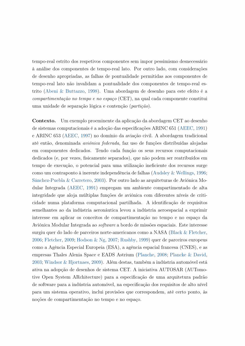
tempo-real estrito dos respetivos componentes sem impor pessimismo desnecessárioà análise dos componentes de tempo-real lato. Por outro lado, com consideraçõesde desenho apropriadas, as falhas de pontualidade permitidas aos componentes detempo-real lato não invalidam a pontualidade dos componentes de tempo-real es-trito (Abeni & Buttazzo, 1998). Uma abordagem de desenho para este efeito é acompartimentação no tempo e no espaço (CET), na qual cada componente constituiuma unidade de separação lógica e contenção (partição).

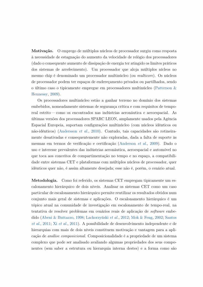
Contexto. Um exemplo proeminente da aplicação da abordagem CET ao desenhode sistemas computacionais é a adoção das especificações ARINC 651 (AEEC, 1991)e ARINC 653 (AEEC, 1997) no domínio da aviação civil. A abordagem tradicionalaté então, denominada aviónica federada, faz uso de funções distribuídas alojadasem componentes dedicados. Tendo cada função os seus recursos computacionaisdedicados (e, por vezes, fisicamente separados), que não podem ser reatribuídos emtempo de execução, o potencial para uma utilização ineficiente dos recursos surgecomo um contraponto à inerente independência de falhas (Audsley & Wellings, 1996;Sánchez-Puebla & Carretero, 2003). Por outro lado as arquiteturas de Aviónica Mo-dular Integrada (AEEC, 1991) empregam um ambiente compartimentado de altaintegridade que aloja múltiplas funções de aviónica com diferentes níveis de criti-cidade numa plataforma computacional partilhada. A identificação de requisitossemelhantes ao da indústria aeronáutica levou a indústria aeroespacial a exprimirinteresse em aplicar os conceitos de compartimentação no tempo e no espaço daAviónica Modular Integrada ao software a bordo de missões espaciais. Este interessesurgiu quer do lado de parceiros norte-americanos como a NASA (Black & Fletcher,2006; Fletcher, 2009; Hodson & Ng, 2007; Rushby, 1999) quer de parceiros europeuscomo a Agência Especial Europeia (ESA), a agência espacial francesa (CNES), e asempresas Thales Alenia Space e EADS Astrium (Planche, 2008; Plancke & David,2003; Windsor & Hjortnaes, 2009). Além destas, também a indústria automóvel estáativa na adopção de desenhos de sistema CET. A iniciativa AUTOSAR (AUTomo-tive Open System ARchitecture) para a especificação de uma arquitetura padrãode software para a indústria automóvel, na especificação dos requisitos de alto nívelpara um sistema operativo, inclui provisões que correspondem, até certo ponto, àsnoções de compartimentação no tempo e no espaço.

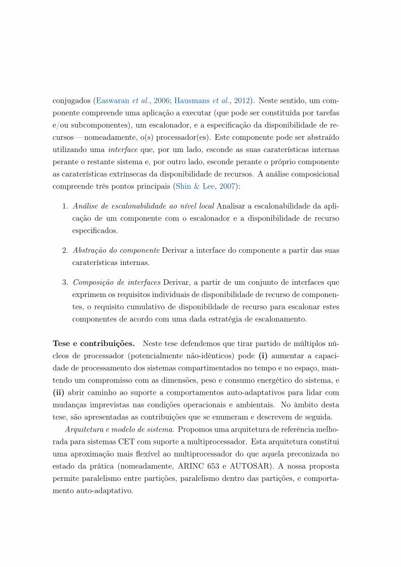
Motivação. O emprego de múltiplos núcleos de processador surgiu como respostaà necessidade de estagnação do aumento da velocidade de relógio dos processadores(dado o consequente aumento de dissipação de energia ter atingido os limites práticosdos sistemas de arrefecimento). Um processador que aloja múltiplos nícleos nomesmo chip é denominado um processador multinúcleo (ou multicore). Os núcleosde processador podem ter espaços de endereçamento privados ou partilhados, sendoo último caso o tipicamente empregue em processadores multinúcleo (Patterson &Hennessy, 2009).

Os processadores multinúcleo estão a ganhar terreno no domínio dos sistemasembebidos, nomeadamente sistemas de segurança crítica e com requisitos de tempo-real estrito—como os encontrados nas indústrias aeronáutica e aeroespacial. Asúltimas versões dos processadores SPARC LEON, amplamente usados pela AgênciaEspacial Europeia, suportam configurações multinúcleo (com núcleos idênticos ounão-idênticos) (Andersson et al., 2010). Contudo, tais capacidades são rotineira-mente desativadas e consequentemente não exploradas, dada a falta de suporte àsmesmas em termos de verificação e certificação (Anderson et al., 2009). Dado ouso e interesse prevalentes das indústrias aeronáutica, aeroespacial e automóvel noque toca aos conceitos de compartimentação no tempo e no espaço, a compatibili-dade entre sistemas CET e plataformas com múltiplos núcleos de processador, queridênticos quer não, é assim altamente desejada; esse não é, porém, o cenário atual.

Metodologia. Como foi referido, os sistemas CET empregam tipicamente um es-calonamento hierárquico de dois níveis. Analisar os sistemas CET como um casoparticular de escalonamento hierárquico permite reutilizar os resultados obtidos numconjunto mais geral de sistemas e aplicações. O escalonamento hierárquico é umtópico atual na comunidade de investigação em escalonamento de tempo-real, natentativa de resolver problemas em cenários reais de aplicação de software embe-dido (Abeni & Buttazzo, 1998; Lackorzyński et al., 2012; Mok & Feng, 2002; Santoset al., 2011; Xi et al., 2011). A possibilidade de desenvolvimento independente e dehierarquias com mais de dois níveis constituem motivação e vantagem para a apli-cação de análise composicional. Composicionalidade é a propriedade de um sistemacomplexo que pode ser analisado avaliando algumas propriedades dos seus compo-nentes (sem saber a estrutura ou hierarquia interna destes) e a forma como são

conjugados (Easwaran et al., 2006; Hausmans et al., 2012). Neste sentido, um com-ponente compreende uma aplicação a executar (que pode ser constituída por tarefase/ou subcomponentes), um escalonador, e a especificação da disponibilidade de re-cursos—nomeadamente, o(s) processador(es). Este componente pode ser abstraídoutilizando uma interface que, por um lado, esconde as suas caraterísticas internasperante o restante sistema e, por outro lado, esconde perante o próprio componenteas caraterísticas extrínsecas da disponibilidade de recursos. A análise composicionalcompreende três pontos principais (Shin & Lee, 2007):

1. Análise de escalonabilidade ao nível local Analisar a escalonabilidade da apli-cação de um componente com o escalonador e a disponibilidade de recursoespecificados.

2. Abstração do componente Derivar a interface do componente a partir das suascaraterísticas internas.

3. Composição de interfaces Derivar, a partir de um conjunto de interfaces queexprimem os requisitos individuais de disponibilidade de recurso de componen-tes, o requisito cumulativo de disponibildade de recurso para escalonar estescomponentes de acordo com uma dada estratégia de escalonamento.

Tese e contribuições. Neste tese defendemos que tirar partido de múltiplos nú-cleos de processador (potencialmente não-idênticos) pode (i) aumentar a capaci-dade de processamento dos sistemas compartimentados no tempo e no espaço, man-tendo um compromisso com as dimensões, peso e consumo energético do sistema, e(ii) abrir caminho ao suporte a comportamentos auto-adaptativos para lidar commudanças imprevistas nas condições operacionais e ambientais. No âmbito destatese, são apresentadas as contribuições que se enumeram e descrevem de seguida.

Arquitetura e modelo de sistema. Propomos uma arquitetura de referência melho-rada para sistemas CET com suporte a multiprocessador. Esta arquitetura constituiuma aproximação mais flexível ao multiprocessador do que aquela preconizada noestado da prática (nomeadamente, ARINC 653 e AUTOSAR). A nossa propostapermite paralelismo entre partições, paralelismo dentro das partições, e comporta-mento auto-adaptativo.

Análise composicional em multiprocessadores uniformes. Propomos o primeiromodelo para interfaces de componentes que permite a definição de hierarquias com-posicionais em multiprocessadores uniformes (aqueles cujos processadores podem sernão-idênticos, mas apenas em termos de velocidade). Esta contribuição permite aanálise formal de sistemas CET com paralelismo entre e/ou dentro das partições emmultiprocessadores potencialmente não-identicos. A nossa contribuição abrange ostrês aspetos da análise composicional de estruturas de escalonamento hierárquico—análise de escalonabilidade ao nível local, abstração do componente, e composição deinterfaces—aplicando e estendendo resultados anteriores de outros autores (Baruah& Goossens, 2008; Easwaran et al., 2009b). Os diferentes aspetos desta contribui-ção são validados analiticamente e demonstrados experimentalmente com recurso asimulação.

Análise, geração e simulação de escalonamento. Apresentamos o desenho e con-cretização do hsSim, uma ferramenta orientada a objetos para simulação e análisede escalonamento e geração de tabelas estáticas de escalonamento. O hsSim foicuidadosamente desenhado com atenção aos padrões de desenho de software apli-cáveis, com objetivos de modularidade, extensibilidade e interoperabilidade. Estaabordagem cuidadosa não é habitualmente aplicada na concretização de utilitáriosde suporte a experiências académicas, sendo esta a principal razão pela qual dese-nhamos uma ferramenta de raíz em vez de modificarmos uma ferramenta existente.Este facto não preclude porém que algumas das contribuições apresentadas sejamimportadas para o código de outras ferramentas, como o Cheddar—que apresentajá bastante maturidade no que respeita à análise e simulação de escalonamento não-hierárquico. Concretizamos o suporte a algoritmos de escalonamento tradicionais,e ainda incorporamos as nossas contribuições no âmbito da análise composicional(teste de escalonabilidade, abstração de componentes, e algoritmo de escalonamentode componentes).

Resultados preliminares sobre auto-adaptação em sistemas CET. Reportamosas experiências levadas a cabo, com um protótipo de sistema CET e através desimulação, para endereçar a segunda parte da tese defendida.

Conclusão e trabalho futuro Nesta tese, abordámos o problema do escalona-mento tempo-real em sistemas compartimentados no tempo e no espaço assentes

sobre processadores multinúcleo. Acrescentámos ao estado da arte a primeira apro-ximação à análise composicional sobre multiprocessadores não-idênticos; os resul-tados formais que desenvolvemos analiticamente são corroborados pelos testes queefetuámos com conjuntos de tarefas gerados aleatoriamente, e são consentâneos comos resultados encontrados na literatura para plataformas multiprocessador dedica-das. Provámos analiticamente que o algoritmo de escalonamento gEDF não asse-gura a composicionalidade na presença de multiprocessadores não-idênticos; paraeste efeito, crucial quando se consideram as vantagens de desenvolvimento e verifi-cação independentes trazidas por abordagens composicionais, propusémos um novoalgoritmo de escalonamento, o umprEDF. Apresentámos também o desenho e desen-volvimento do hsSim, uma ferramenta orientada a objetos para análise, simulação egeração de tabelas de escalonamento; o hsSim será disponibilizado como ferramentade código aberto para usufruto da comunidade de investigação em escalonamentotempo-real, e é uma prova de conceito para a inclusão de suporte a escalonamentohierárquico numa ferramenta mais madura. Usámos o hsSim para mostrar em acçãoos métodos formais que apresentámos.

Panorama de aplicabilidade. O modelo de sistema utilizado contém assunçõesrelacionadas com o impacto temporal de fenómenos relacionados com o hardware(preempção e migração de tarefas, contenção no barramento, memória cache). Estaassunção é comum na investigação em escalonamento tempo-real, e não é totalmentedíspar da realidade (Jalle et al., 2013; Jean et al., 2012); iremos porém, no futuro,olhar com mais detalhe para este impacto temporal.

Ao longo dos anos, houve vários projetos de investigação, financiados por enti-dades europeias, a empregar abordagens baseadas em componentes e/ou comparti-mentação no tempo e no espaço para atingir hibridização arquitetual ou lidar comsistemas de criticidade mista (exemplos: ACTORS, RECOMP, KARYON). Em al-guns destes projetos, essencialmente contemporâneos com o trabalho desta tese, osprocessadores multinúcleo são abordados até certo ponto. O trabalho apresentadonesta tese é aplicável às arquiteturas consideradas em ou resultantes destes projetos,endereçando até aspetos deixados em aberto no final dos mesmos. Em particular, osnossos resultados transpõem a fasquia destes projetos no que respeita ao paralelismoentre componentes e ao uso de processadores não-idênticos. No domínio aeroespa-cial, os amplamente usados processadores SPARC LEON permitem configurações

com núcleos de processador não-idênticos, mas a falta de suporte de sistema opera-tivo tem desencorajado o seu aproveitamento.

Além do inicialmente estabelecido foco em domínio de aplicação críticos, osnossos resultados também contribuem para a verificação formal de sistemas ba-seados emc omponentes assentes multiprocessadores não-idênticos como o Cell e obig.LITTLE. Embora estes não sejam tipicamente empregues em domínios críticos,aplicar uma abordagem baseada em componentes ao desenvolvimento de softwarecomplexo para executar sobre os mesmos permite reduzir a complexidade e custodeste processo, enquanto se assegura que os componentes individuais tem garantiasmínimas de qualidade de serviço. Tal será particularmente verdade à medida queo suporte de sistema operativo ao escalonamento hierárquico aumenta (Abdullahet al., 2013; Bini et al., 2011b).

Trabalho futuro. As vias de trabalho futuro relacionado com a presente tese queidentificamos desde já incluem (i) suporte de hardware e assunções do modelo desistema; (ii) algoritmos de escalonamento; (iii) análise composicional com garan-tias temporais variadas, como sejam tempo-real lato e escalonamento de criticidademista; e (iv) reconfiguração e tolerâncias a faltas proativa.

Acknowledgments

Although individually authored, this dissertation owes its completion to the support ofquite some people. I now take the opportunity to thank them.

To my advisor José Rufino, for his full scientific, institutional and personal support.I particularly praise the attention to detail with which he scrutinized the papers we co-wrote (and the drafts of this dissertation), the concern he puts in providing adequate andfair conditions for his students to carry on their work, and how he strives to give hisPhD students the proper training for independent research by assigning complementaryresponsibilities (such as reviewing papers, and actively participating in the elaboration ofproject funding proposals).

To FCUL Professors André Falcão, Isabel Nunes, Luís Correia, Mário Calha, Pedro M.Ferreira and Vasco T. Vasconcelos, and to IST Professor Leonel Sousa, for the insightfulcomments I received at the different stages of evaluation of my work.

To the SAPIENT team at Lab-STICC (Université de Bretagne Occidentale, Brest,France), especially Laurent Lemarchand, Vincent Gaudel, and Frank Singhoff. The collab-oration and idea exchanges within the SAPIENT project had a great influence in the waysome parts of this work were conducted.

To LaSIGE and the Department of Informatics, for enabling such a lively and stimu-lating environment for learning, researching and teaching. To the Navigators group in gen-eral, and more specifically to the TADS research line leaders Paulo Verissimo and AntónioCasimiro and to the “Toutiçanos” with whom I most closely collaborated: Jeferson Souza,Joaquim Rosa, Kleomar Almeida, Pedro Nóbrega da Costa, Ricardo Pinto, Rui PedroCaldeira and Rui Silveira.

For the less work-oriented companionship, to my regular LaSIGE office and lunch matesLuís Duarte, Nádia Fernandes, Tiago Gonçalves, and—finally and specially—José Bap-tista Coelho. More than a colleague, José has been true friend for all occasions, enablingme to behave more like a human being than I was used to.

To my mother Mafalda, my sister Joana and my “sister” Sophie, for having been always,since way back in time, a permanent source of comfort and support.

Last but not least, to Catarina, my love. For having endured my periods of absence,unavailability, frustration, impatience and mood swings, and for countering them withcopious amounts of love, dedication, understanding and good moments, you definitelydeserve the dedication of this dissertation.

João Pedro Gonçalves Crespo CraveiroLisbon, August 2013

Para a minha querida Catarina.Para o Nós.

“Vogons!” snapped Ford, “we’re under attack!”

Arthur gibbered.

“Well what are you doing? Let’s get out of here!”

“Can’t. Computer’s jammed. [...] It says all its circuits are occupied.”[...]

“Tell me ... did the computer say what was occupying it? I just ask outof interest ...”

[...] “I think a short while ago it was trying to work out how to ... makeme some tea.”

“That’s right guys,” the computer sang out suddenly, “just coping withthat problem right now, and wow, it’s a biggy. Be with you in a while.”It lapsed back into a silence that was only matched for sheer intensityby the silence of the three people staring at Arthur Dent.

As if to relieve the tension, the Vogons chose that moment to start firing.

—Douglas Adams (1980). The Restaurant at the End of theUniverse. Pan Books.

Contents

List of Figures v

List of Tables vii

List of Theorems ix

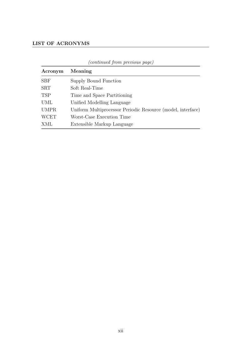
List of Acronyms xi

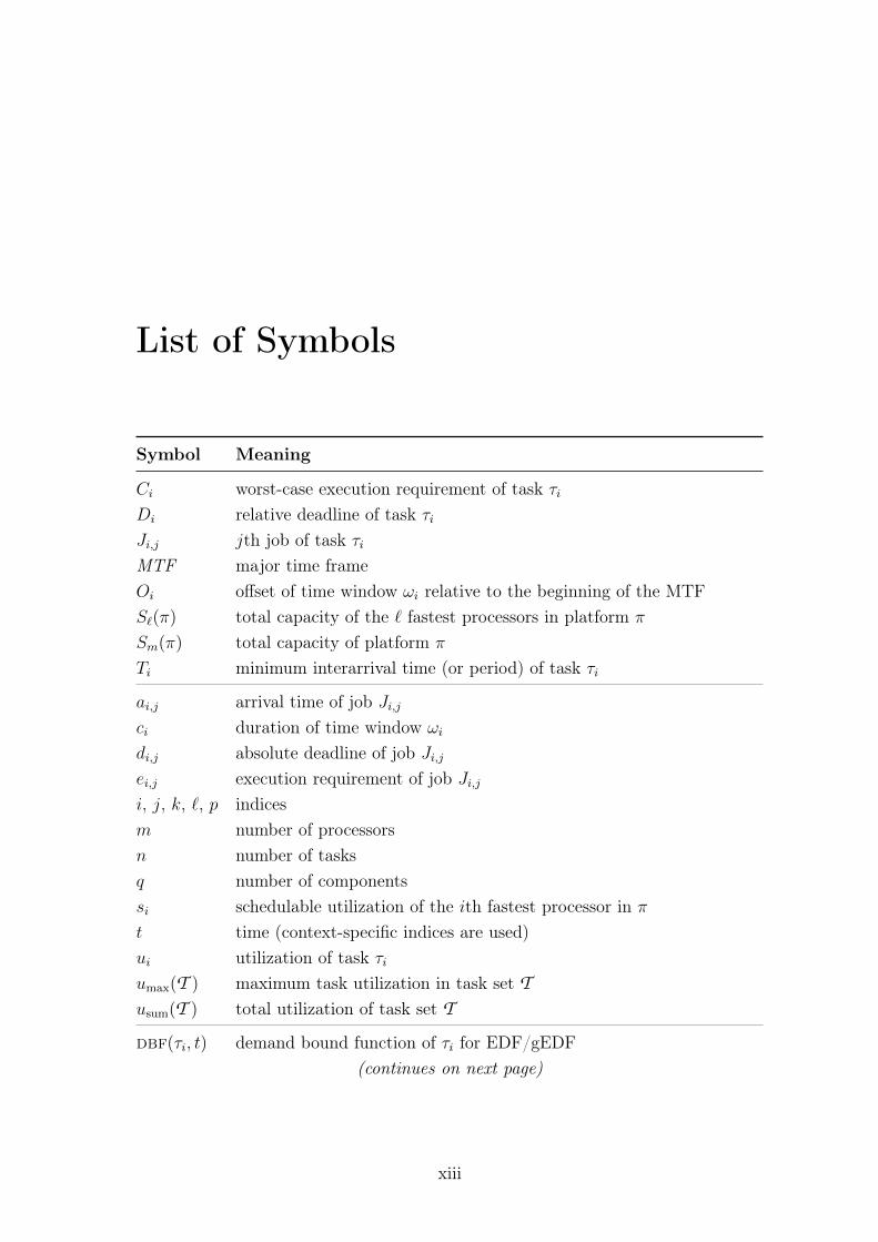
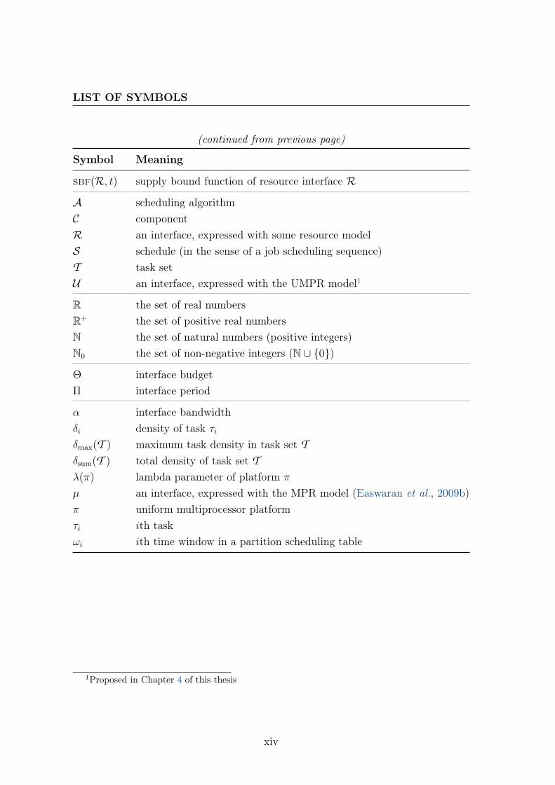
List of Symbols xiii

Publications xv

1 Introduction 11.1 Context . . . . . . . . . . . . . . . . . . . . . . . . . . . . . . . . . . 2

1.1.1 Civil aviation . . . . . . . . . . . . . . . . . . . . . . . . . . . 21.1.2 Aerospace . . . . . . . . . . . . . . . . . . . . . . . . . . . . . 51.1.3 Automotive industry . . . . . . . . . . . . . . . . . . . . . . . 6

1.2 Motivation . . . . . . . . . . . . . . . . . . . . . . . . . . . . . . . . . 71.3 Thesis statement . . . . . . . . . . . . . . . . . . . . . . . . . . . . . 81.4 Methodology . . . . . . . . . . . . . . . . . . . . . . . . . . . . . . . 91.5 Contributions . . . . . . . . . . . . . . . . . . . . . . . . . . . . . . . 101.6 Document outline . . . . . . . . . . . . . . . . . . . . . . . . . . . . . 12

2 Background and Related Work 132.1 Real-time scheduling background . . . . . . . . . . . . . . . . . . . . 13

2.1.1 Task models . . . . . . . . . . . . . . . . . . . . . . . . . . . . 142.1.2 Platform models . . . . . . . . . . . . . . . . . . . . . . . . . 17

i

CONTENTS

2.1.3 Scheduling algorithm classification . . . . . . . . . . . . . . . 182.1.4 Schedulability analysis notions . . . . . . . . . . . . . . . . . . 19

2.2 Hard real-time scheduling on dedicated platforms . . . . . . . . . . . 202.2.1 Scheduling on uniprocessor platforms . . . . . . . . . . . . . . 202.2.2 Partitioned scheduling on identical multiprocessors . . . . . . 222.2.3 Global scheduling on identical multiprocessors . . . . . . . . . 242.2.4 Global scheduling on uniform multiprocessors . . . . . . . . . 28

2.3 Scheduling approaches for mixed systems . . . . . . . . . . . . . . . . 292.3.1 Resource reservation frameworks . . . . . . . . . . . . . . . . 292.3.2 Hierarchical scheduling frameworks (HSF) . . . . . . . . . . . 32

2.4 Compositional analysis . . . . . . . . . . . . . . . . . . . . . . . . . . 352.4.1 Common definitions . . . . . . . . . . . . . . . . . . . . . . . 372.4.2 Uniprocessor . . . . . . . . . . . . . . . . . . . . . . . . . . . 382.4.3 Identical multiprocessor . . . . . . . . . . . . . . . . . . . . . 42

2.5 Technological support to TSP . . . . . . . . . . . . . . . . . . . . . . 482.5.1 Operating system support . . . . . . . . . . . . . . . . . . . . 482.5.2 Scheduling analysis and simulation tools . . . . . . . . . . . . 52

2.6 Summary . . . . . . . . . . . . . . . . . . . . . . . . . . . . . . . . . 54

3 Architecture and Model for Multiprocessor Time- and Space-Partitioned Systems 573.1 Architecture overview . . . . . . . . . . . . . . . . . . . . . . . . . . . 57

3.1.1 Architecture components . . . . . . . . . . . . . . . . . . . . . 583.1.2 Achieving time partitioning . . . . . . . . . . . . . . . . . . . 59

3.2 Evolution for multiprocessor . . . . . . . . . . . . . . . . . . . . . . . 613.2.1 Interpartition parallelism . . . . . . . . . . . . . . . . . . . . . 633.2.2 Intrapartition parallelism . . . . . . . . . . . . . . . . . . . . . 633.2.3 Enhanced spatial partitioning . . . . . . . . . . . . . . . . . . 643.2.4 Self-adaptive fault tolerance . . . . . . . . . . . . . . . . . . . 64

3.3 TSP system model . . . . . . . . . . . . . . . . . . . . . . . . . . . . 653.3.1 Platform model . . . . . . . . . . . . . . . . . . . . . . . . . . 663.3.2 Component model . . . . . . . . . . . . . . . . . . . . . . . . 663.3.3 Global-level scheduling . . . . . . . . . . . . . . . . . . . . . . 68

ii

CONTENTS

3.4 Summary . . . . . . . . . . . . . . . . . . . . . . . . . . . . . . . . . 68

4 Compositional Analysis on (Non-)Identical UniformMultiprocessors 714.1 Resource model . . . . . . . . . . . . . . . . . . . . . . . . . . . . . . 71

4.1.1 Supply bound function . . . . . . . . . . . . . . . . . . . . . . 734.1.2 Linear lower bound on the supply bound function . . . . . . . 75

4.2 Local-level schedulability analysis . . . . . . . . . . . . . . . . . . . . 764.2.1 Interference interval . . . . . . . . . . . . . . . . . . . . . . . . 774.2.2 Component demand . . . . . . . . . . . . . . . . . . . . . . . 794.2.3 Sufficient local-level schedulability test . . . . . . . . . . . . . 82

4.3 Component abstraction . . . . . . . . . . . . . . . . . . . . . . . . . . 844.3.1 Minimum resource interface . . . . . . . . . . . . . . . . . . . 854.3.2 Uniform vs. identical multiprocessor platform . . . . . . . . . 854.3.3 Number of processors . . . . . . . . . . . . . . . . . . . . . . . 874.3.4 Simulation experiments . . . . . . . . . . . . . . . . . . . . . . 88

4.4 Intercomponent scheduling . . . . . . . . . . . . . . . . . . . . . . . . 944.4.1 Transforming components to interface tasks . . . . . . . . . . 944.4.2 Compositionality with gEDF intercomponent scheduling . . . 994.4.3 The umprEDF algorithm for intercomponent scheduling . . . . 1014.4.4 Interface composition . . . . . . . . . . . . . . . . . . . . . . . 102

4.5 Summary . . . . . . . . . . . . . . . . . . . . . . . . . . . . . . . . . 104

5 Scheduling Analysis, Generation and Simulation Tool 1075.1 Object-oriented analysis and design . . . . . . . . . . . . . . . . . . . 107

5.1.1 Domain analysis . . . . . . . . . . . . . . . . . . . . . . . . . . 1085.1.2 n-level hierarchy: the Composite pattern . . . . . . . . . . . . 1085.1.3 Scheduling algorithm encapsulation: the Strategy pattern . . . 1105.1.4 n -level hierarchy and polymorphism . . . . . . . . . . . . . . 1115.1.5 Decoupling the simulation from the simulated domain using

the Observer and Visitor patterns . . . . . . . . . . . . . . . . 1135.1.6 Multiprocessor schedulers . . . . . . . . . . . . . . . . . . . . 1155.1.7 Interfaces aiding scheduling analysis . . . . . . . . . . . . . . . 1165.1.8 Compositional analysis with the Decorator pattern . . . . . . 117

iii

CONTENTS

5.2 Implementation . . . . . . . . . . . . . . . . . . . . . . . . . . . . . . 1185.2.1 Extensions . . . . . . . . . . . . . . . . . . . . . . . . . . . . . 118

5.3 Example use case . . . . . . . . . . . . . . . . . . . . . . . . . . . . . 1215.3.1 Scheduling analysis . . . . . . . . . . . . . . . . . . . . . . . . 1215.3.2 Scheduling simulation and visualization . . . . . . . . . . . . . 1215.3.3 Schedule generation . . . . . . . . . . . . . . . . . . . . . . . . 125

5.4 Summary . . . . . . . . . . . . . . . . . . . . . . . . . . . . . . . . . 125

6 Towards Self-Adaptation in Time- and Space-Partitioned Systems 1296.1 Monitoring and adaptation mechanisms . . . . . . . . . . . . . . . . . 129

6.1.1 Task deadline violation monitoring . . . . . . . . . . . . . . . 1306.1.2 Mode-based schedules . . . . . . . . . . . . . . . . . . . . . . 1336.1.3 Prototype implementation . . . . . . . . . . . . . . . . . . . . 1356.1.4 Evaluation . . . . . . . . . . . . . . . . . . . . . . . . . . . . . 136

6.2 Self-adaptation upon temporal faults . . . . . . . . . . . . . . . . . . 1386.2.1 Evaluation . . . . . . . . . . . . . . . . . . . . . . . . . . . . . 139

6.3 Improvements discussion . . . . . . . . . . . . . . . . . . . . . . . . . 1426.3.1 Multiprocessor . . . . . . . . . . . . . . . . . . . . . . . . . . 1436.3.2 Reconfiguration . . . . . . . . . . . . . . . . . . . . . . . . . . 1436.3.3 Proactivity . . . . . . . . . . . . . . . . . . . . . . . . . . . . 144

6.4 Summary . . . . . . . . . . . . . . . . . . . . . . . . . . . . . . . . . 144

7 Conclusion and Future Work 1457.1 Applicability perspective . . . . . . . . . . . . . . . . . . . . . . . . . 1467.2 Future work . . . . . . . . . . . . . . . . . . . . . . . . . . . . . . . . 148

7.2.1 Hardware support and system model assumptions . . . . . . . 1497.2.2 Scheduling algorithms . . . . . . . . . . . . . . . . . . . . . . 1497.2.3 Compositional analysis . . . . . . . . . . . . . . . . . . . . . . 1507.2.4 Reconfiguration and proactivity . . . . . . . . . . . . . . . . . 151

References 153

iv

List of Figures

1.1 Basic architecture of an IMA computing module . . . . . . . . . . . . 3

1.2 Standard ARINC 653 architecture . . . . . . . . . . . . . . . . . . . . 4

2.1 Execution pattern considered in Baker (2003)’s proof and thereoninspired works. . . . . . . . . . . . . . . . . . . . . . . . . . . . . . . 26

2.2 Resource reservation framework . . . . . . . . . . . . . . . . . . . . . 30

2.3 Hierarchical scheduling framework . . . . . . . . . . . . . . . . . . . . 32

2.4 Compositional scheduling framework . . . . . . . . . . . . . . . . . . 36

2.5 Minimum supply schedule for an MPR interface µ = (Π,Θ,m) . . . . 42

3.1 Architecture overview . . . . . . . . . . . . . . . . . . . . . . . . . . . 58

3.2 Two-level scheduling scheme . . . . . . . . . . . . . . . . . . . . . . . 59

3.3 Example comparison between a multiprocessor system implementedas interconnected uniprocessor TSP nodes, and a multicore (or shared-memory multiprocessor) TSP system implemented with our proposalof an evolved architecture . . . . . . . . . . . . . . . . . . . . . . . . 61

3.4 Interpartition parallelism example timeline . . . . . . . . . . . . . . . 63

3.5 Example timeline with a combination of both inter- and intrapartitionparallelism . . . . . . . . . . . . . . . . . . . . . . . . . . . . . . . . . 64

3.6 Fault tolerance example timeline . . . . . . . . . . . . . . . . . . . . . 65

3.7 Example timeline showing a combination of fault tolerance with inter-and intrapartition parallelism . . . . . . . . . . . . . . . . . . . . . . 65

3.8 System model . . . . . . . . . . . . . . . . . . . . . . . . . . . . . . . 66

4.1 Compositional scheduling framework with the UMPR . . . . . . . . . 72

v

LIST OF FIGURES

4.2 Minimum supply schedule for two UMPR interfaces: U = (Π,Θ, π)

and U ′ = (Π,Θ, π′), where Sm(π) > Sm(π′) (both with m processors) 744.3 Plot of sbf and lsbf for U and U ′ . . . . . . . . . . . . . . . . . . . 764.4 Considered execution pattern. . . . . . . . . . . . . . . . . . . . . . . 774.5 Comparison between minimal bandwidth for UMPRs based on iden-

tical and non-identical uniform multiprocessors. . . . . . . . . . . . . 904.6 Success rates for MPR and UMPR interfaces with identical multipro-

cessor platforms. . . . . . . . . . . . . . . . . . . . . . . . . . . . . . 924.7 Average overhead for MPR and UMPR interfaces with identical mul-

tiprocessor platforms. . . . . . . . . . . . . . . . . . . . . . . . . . . . 934.8 Formalization of umprEDF with pseudocomponents . . . . . . . . . . 101

5.1 Traditional 1-level system domain model . . . . . . . . . . . . . . . . 1085.2 2-level hierarchical scheduling system domain model . . . . . . . . . . 1095.3 n-level hierarchical scheduling system using the Composite pattern . . 1105.4 Scheduling algorithm encapsulation with the Strategy pattern . . . . 1115.5 Sequence diagram for the scheduler tickle operation . . . . . . . . . . 1125.6 Application of the Observer pattern for loggers . . . . . . . . . . . . . 1145.7 Application of the Visitor pattern for loggers . . . . . . . . . . . . . . 1145.8 Multiprocessor schedulers . . . . . . . . . . . . . . . . . . . . . . . . 1155.9 Interfaces implemented by the periodic and sporadic task classes. . . 1165.10 Support for compositional analysis with the Decorator pattern . . . . 1185.11 Worst-case response time . . . . . . . . . . . . . . . . . . . . . . . . . 1235.12 Grasp trace of the simulation with gEDF global-level scheduling. . . . 1235.13 Grasp trace of the simulation with umprEDF global-level scheduling. . 1245.14 Grasp trace for the simulation of task set T1∪T2 being scheduled with

gEDF directly on the physical platform. . . . . . . . . . . . . . . . . 125

6.1 Deadline violation monitoring example . . . . . . . . . . . . . . . . . 1316.2 Screenshot of the Intel IA-32 prototype of the AIR architecture. . . . 1356.3 Example . . . . . . . . . . . . . . . . . . . . . . . . . . . . . . . . . . 1416.4 Simulation results: deadline miss rate; deadline misses over time . . . 142

vi

List of Tables

4.1 Success rates of MPR and UMPR interfaces with identical multipro-cessor platforms (among feasible cases). . . . . . . . . . . . . . . . . . 92

5.1 Mapping between hsSim events and Grasp trace content. . . . . . . . 119

6.1 APEX services in need of modifications to support task deadline vi-olation monitoring . . . . . . . . . . . . . . . . . . . . . . . . . . . . 132

6.2 Essential APEX services for Health Monitoring . . . . . . . . . . . . 1326.3 Essential APEX services to support mode-based schedules . . . . . . 1356.4 Logical SLOC and cyclomatic complexity (CC) for the AIR Partition

Scheduler with mode-based schedules . . . . . . . . . . . . . . . . . . 1366.5 Logical SLOC and cyclomatic complexity (CC) for the implementa-

tion of deadline violation monitoring in AIR PAL . . . . . . . . . . . 1376.6 AIR Partition Scheduler (with mode-based schedules) execution time

— basic metrics . . . . . . . . . . . . . . . . . . . . . . . . . . . . . . 138

vii

List of Theorems

4.1 Theorem (Sufficient gEDF-schedulability test for the UMPR) . . . . . 834.2 Theorem (Superiority of less identical platforms) . . . . . . . . . . . . 874.3 Theorem (Superiority of platforms with less processors) . . . . . . . . 884.4 Theorem (Generalization of the task transformation for the MPR) . . 954.5 Theorem (Correctness of the transformation to interface tasks) . . . . 984.6 Theorem (Inadequacy of gEDF for intercomponent scheduling) . . . . 1004.7 Theorem (Adequacy of umprEDF for intercomponent scheduling) . . . 102

ix

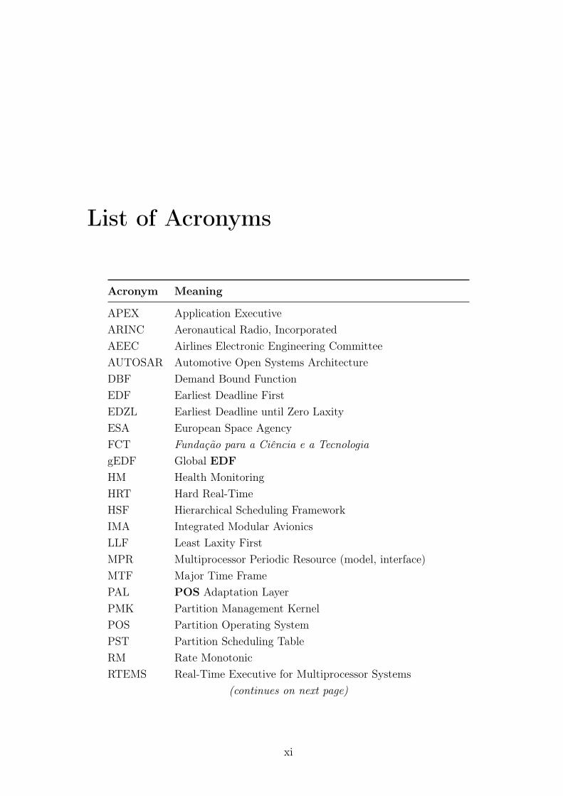
List of Acronyms

Acronym Meaning

APEX Application ExecutiveARINC Aeronautical Radio, IncorporatedAEEC Airlines Electronic Engineering CommitteeAUTOSAR Automotive Open Systems ArchitectureDBF Demand Bound FunctionEDF Earliest Deadline FirstEDZL Earliest Deadline until Zero LaxityESA European Space AgencyFCT Fundação para a Ciência e a TecnologiagEDF Global EDFHM Health MonitoringHRT Hard Real-TimeHSF Hierarchical Scheduling FrameworkIMA Integrated Modular AvionicsLLF Least Laxity FirstMPR Multiprocessor Periodic Resource (model, interface)MTF Major Time FramePAL POS Adaptation LayerPMK Partition Management KernelPOS Partition Operating SystemPST Partition Scheduling TableRM Rate MonotonicRTEMS Real-Time Executive for Multiprocessor Systems

(continues on next page)

xi

LIST OF ACRONYMS

(continued from previous page)

Acronym Meaning

SBF Supply Bound FunctionSRT Soft Real-TimeTSP Time and Space PartitioningUML Unified Modelling LanguageUMPR Uniform Multiprocessor Periodic Resource (model, interface)WCET Worst-Case Execution TimeXML Extensible Markup Language

xii

List of Symbols

Symbol Meaning

Ci worst-case execution requirement of task τiDi relative deadline of task τiJi,j jth job of task τiMTF major time frameOi offset of time window ωi relative to the beginning of the MTFS`(π) total capacity of the ` fastest processors in platform π

Sm(π) total capacity of platform π

Ti minimum interarrival time (or period) of task τi

ai,j arrival time of job Ji,jci duration of time window ωi

di,j absolute deadline of job Ji,jei,j execution requirement of job Ji,ji, j, k, `, p indicesm number of processorsn number of tasksq number of componentssi schedulable utilization of the ith fastest processor in πt time (context-specific indices are used)ui utilization of task τiumax(T ) maximum task utilization in task set Tusum(T ) total utilization of task set T

dbf(τi, t) demand bound function of τi for EDF/gEDF(continues on next page)

xiii

LIST OF SYMBOLS

(continued from previous page)

Symbol Meaning

sbf(R, t) supply bound function of resource interface R

A scheduling algorithmC componentR an interface, expressed with some resource modelS schedule (in the sense of a job scheduling sequence)T task setU an interface, expressed with the UMPR model1

R the set of real numbersR+ the set of positive real numbersN the set of natural numbers (positive integers)N0 the set of non-negative integers (N ∪ {0})

Θ interface budgetΠ interface period

α interface bandwidthδi density of task τiδmax(T ) maximum task density in task set Tδsum(T ) total density of task set Tλ(π) lambda parameter of platform π

µ an interface, expressed with the MPR model (Easwaran et al., 2009b)π uniform multiprocessor platformτi ith taskωi ith time window in a partition scheduling table

1Proposed in Chapter 4 of this thesis

xiv

Publications

The contributions of this thesis have been reported, partially and in preliminaryversions, in the following publications.

Book chapters

Craveiro, J., Rufino, J. & Verissimo, P. (2010a). Architecting robustness andtimeliness in a new generation of aerospace systems. In A. Casimiro, R. de Lemos& G. Gacek, eds., Architecting Dependable Systems VII, vol. 6420 of Lecture Notesin Computer Science, 146–170, Springer Berlin / Heidelberg.DOI: 10.1007/978-3-642-17245-8_7

Journals

Craveiro, J., Rufino, J. & Singhoff, F. (2011a). Architecture, mechanismsand scheduling analysis tool for multicore time- and space-partitioned systems. ACMSIGBED Review, 8(3):23–27, special issue of the 23rd Euromicro Conference onReal-Time Systems (ECRTS ’11) Work-in-Progress session.DOI: 10.1145/2038617.2038622.

Formal proceedings of international conferences

Craveiro, J. & Rufino, J. (2010b). Schedulability analysis in partitioned systemsfor aerospace avionics. In 15th Internacional Conference on Emerging Technologiesand Factory Automation (ETFA 2010), Bilbao, Spain.DOI: 10.1109/ETFA.2010.5641243

xv

PUBLICATIONS

Rufino, J. & Craveiro, J. & Verissimo, P. (2010b). Building a time- and

space-partitioned architecture for the next generation of space vehicle avionics. In

8th IFIP Workshop on Software Technologies for Future Embedded and Ubiquitous

Systems (SEUS 2010), 179–190, Waidhofen an der Ybbs, Austria.

DOI: 10.1007/978-3-642-16256-5_18

Craveiro, J. & Rufino, J. (2010a). Adaptability support in time- and space-

partitioned aerospace systems. In 2nd International Conference on Adaptive and

Self-adaptive Systems and Applications (ADAPTIVE 2010), 152–157, Lisbon, Por-

tugal.

ISBN: 978-1-61208-109-0

Rosa, J., Craveiro, J. & Rufino, J. (2011). Safe online reconfiguration of time-

and space-partitioned systems. In 9th IEEE International Conference on Industrial

Informatics (INDIN 2011), Caparica, Lisbon, Portugal.

DOI: 10.1109/INDIN.2011.6034932

Informal proceedings, national conferences

Craveiro, J.P., Rosa, J. & Rufino, J. (2011b). Towards self-adaptive schedul-

ing in time- and space-partitioned systems. In 32nd IEEE Real-Time Systems Sym-

posium (RTSS 2011) Work-in-Progress session, Vienna, Austria.

Craveiro, J.P., Silveira, R.O. & Rufino, J. (2012a). hsSim: an extensible

interoperable object-oriented n-level hierarchical scheduling simulator. In 3rd Inter-

national Workshop on Analysis Tools and Methodologies for Embedded and Real-time

Systems (WATERS 2012), Pisa, Italy.

Craveiro, J.P., Souza, J.L.R., Rufino, J., Gaudel, V., Lemarchand, L.,

Plantec, A., Rubini, S. & Singhoff, F. (2012b). Scheduling analysis principles

and tool for time- and space-partitioned systems. In INFORUM 2012 - Simpósio de

Informática, Lisbon, Portugal.

Craveiro, J.P. & Rufino, J. (2013b). Uniform Multiprocessor Periodic Re-

source Model. In 4th International Real-Time Scheduling Open Problems Seminar

(RTSOPS 2013), Paris, France.

xvi

Technical reports

Craveiro, J.P. & Rufino, J. (2012). Towards compositional hierarchical schedul-ing frameworks on uniform multiprocessors. Tech. Rep. TR-2012-08, University ofLisbon, DI–FCUL, revised January 2013.

xvii

Chapter 1

Introduction

A real-time (computing) system is a computing system such that its computations’correctness (or utility) is defined, not only in terms of the accuracy of the logi-cal results, but also in terms of the time at which these results are provided. Therelationship between the timeliness of result provision and their utility allows consid-ering different classes of real-time. Real-time systems have been classically dividedinto hard real-time (HRT) systems and soft real-time (SRT) systems. An HRT sys-tem contains, at least, an HRT task—a task which must always meet its timelinessrequirements (deadline); otherwise, the results of that task’s computation have noutility. HRT systems are usually associated with applications where failure to meettemporal constraints may cause catastrophical effects, including the loss of humanlives or harm thereto. An SRT system contains no HRT tasks, but contains atleast an SRT task—a task which should meet its timeliness requirements, but mayoccasionally miss them (in which case the utility of the result degrades throughtime). SRT systems are usually associated with applications where the beneficialoutcome from the observance of temporal constraints lies within the spectrum ofuser experience, or comfort. Research on real-time systems has focused on the setof algorithms and analysis techniques which allow system developers to know, priorto the system’s deployment and execution, if it will be able to guarantee the fulfill-ment of its timeliness requirements (either HRT or SRT) (Kopetz, 1997; Verissimo& Rodrigues, 2001).

Computing systems have evolved throughout the years to meet various needs,including concerns about size, weight and power consumption (and, consequently,

1

1. Introduction

cost). This led to a trend towards integrating separate systems as subsystems ofa more complex mixed-criticality system on a common computing platform. Suchsystem features the coexistence of different classes of real-time (SRT and HRT), andsubsystems which may be developed by different teams and with different levels ofassurance. The classical approach, often called federated, was to host each of thesesubsystems in separate communicating nodes with dedicated resources—with theconsequent added weight and cost of computing hardware and cables. The addedcomplexity of the system propagates to system’s development, testing, validationand maintenance activities. Designing such complex systems around the notion ofcomponent, thus allowing component-based analysis, brings several benefits, somespecific to real-time systems (Lipari et al., 2005; Lorente et al., 2006). In the caseof different classes of real-time, the advantages of keeping the SRT and HRT partsof the system logically separated (and analyzing them as such) are twofold. Onthe one hand, the separate analysis allows fulfilling the HRT requirements of suchcomponents without imposing unnecessary pessimism on the analysis of the SRTcomponents. On the other hand, with appropriate design considerations, the tar-diness permitted to the SRT components shall not void the timeliness of the HRTcomponents (Abeni & Buttazzo, 1998). One such design approach is time andspace partitioning (TSP). Each component is hosted on a logical separation andcontainment unit— partition. In a TSP system, the various onboard functions areintegrated in a shared computing platform, however being logically separated intopartitions. Robust temporal and spatial partitioning means that partitions do notmutually interfere in terms of fulfillment of real-time and addressing space encapsu-lation requirements.

1.1 Context

1.1.1 Civil aviation

A prominent example of TSP system design is the adoption of the ARINC specifica-tions 651—Design Guidance for Integrated Modular Avionics (AEEC, 1991)—and653—Avionics Application Software Standard Interface (AEEC, 1997)— in the avi-ation and aerospace domains.

2

1.1 Context

Hardware

Application Interface Layer

Partition A Partition B

Operating System

Hardware Interface Layer

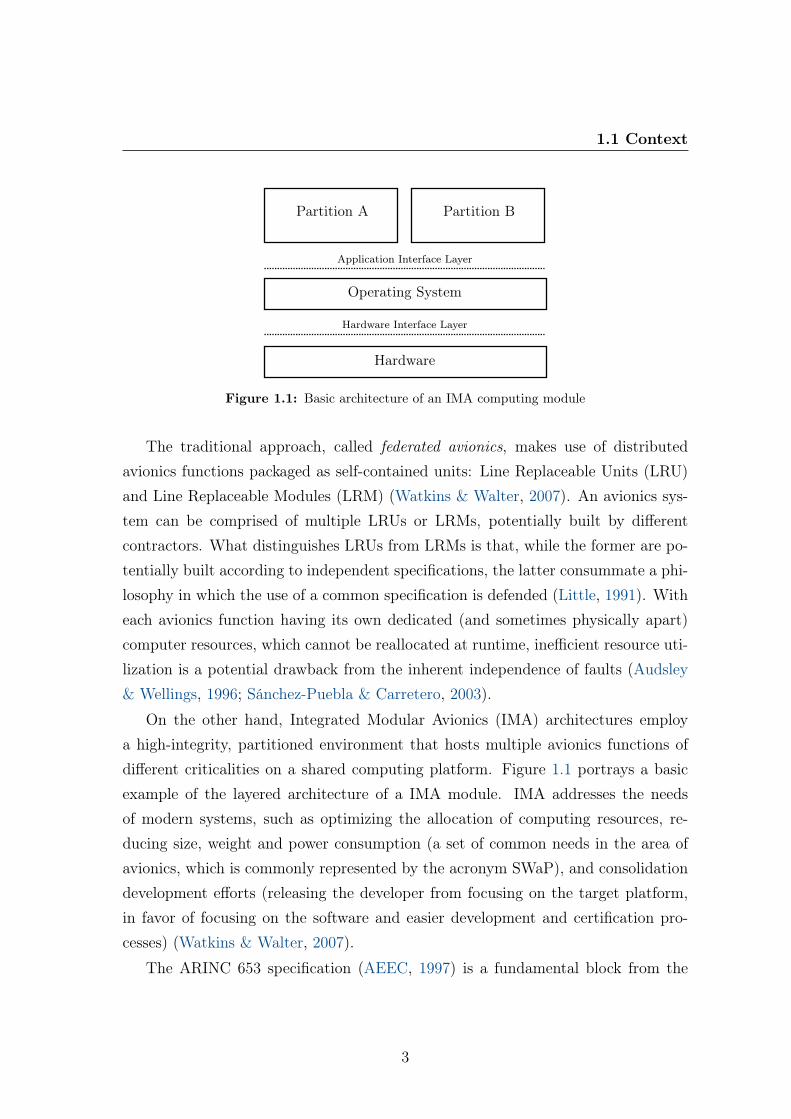
Figure 1.1: Basic architecture of an IMA computing module

The traditional approach, called federated avionics, makes use of distributedavionics functions packaged as self-contained units: Line Replaceable Units (LRU)and Line Replaceable Modules (LRM) (Watkins & Walter, 2007). An avionics sys-tem can be comprised of multiple LRUs or LRMs, potentially built by differentcontractors. What distinguishes LRUs from LRMs is that, while the former are po-tentially built according to independent specifications, the latter consummate a phi-losophy in which the use of a common specification is defended (Little, 1991). Witheach avionics function having its own dedicated (and sometimes physically apart)computer resources, which cannot be reallocated at runtime, inefficient resource uti-lization is a potential drawback from the inherent independence of faults (Audsley& Wellings, 1996; Sánchez-Puebla & Carretero, 2003).

On the other hand, Integrated Modular Avionics (IMA) architectures employa high-integrity, partitioned environment that hosts multiple avionics functions ofdifferent criticalities on a shared computing platform. Figure 1.1 portrays a basicexample of the layered architecture of a IMA module. IMA addresses the needsof modern systems, such as optimizing the allocation of computing resources, re-ducing size, weight and power consumption (a set of common needs in the area ofavionics, which is commonly represented by the acronym SWaP), and consolidationdevelopment efforts (releasing the developer from focusing on the target platform,in favor of focusing on the software and easier development and certification pro-cesses) (Watkins & Walter, 2007).

The ARINC 653 specification (AEEC, 1997) is a fundamental block from the

3

1. Introduction

Hardware

APEX Interface

OS Kernel System-specificfunctions

ApplicationPartition 1 ...

Application Software Layer

Core Software Layer

ApplicationPartition N

SystemPartition 1 ... System

Partition K

Figure 1.2: Standard ARINC 653 architecture—adapted from (AEEC, 1997)

IMA definition, where the partitioning concept emerges for protection and functionalseparation between applications, usually for fault containment and ease of validation,verification, and certification (AEEC, 1997; Rushby, 1999).

The architecture of a standard ARINC 653 system is sketched in Figure 1.2. Atthe application software layer, each application is executed in a confined context—apartition. The application software layer may include system partitions intended tomanage interactions with specific hardware devices. Application partitions consistin general of one or more processes and can only use the services provided by a logicalapplication executive (APEX) interface, as defined in the ARINC 653 specification(AEEC, 1997). System partitions may use also specific functions provided by thecore software layer (e.g. hardware interfacing and device drivers), being allowed tobypass the standard APEX interface.

The ARINC 653 specification defines a standard interface between the softwareapplications and the underlying operating system, known as application executive(APEX) interface. The first part of the specification (AEEC, 1997) describes a set ofmandatory services, concerning partition management, process management, timemanagement, intrapartition communication (i.e., between processes in the same par-tition), interpartition communication (i.e., between processes in different partitions),and health monitoring. The Part 2 of the ARINC 653 specification (AEEC, 2007)

4

1.1 Context

adds, to the aforementioned mandatory services, optional services or extensions tothe required services.

In ARINC 653 TSP systems, time partitioning is typically guaranteed by a two-level scheduler (AEEC, 1997). On the first level, partitions are selected to executeaccording to some schedule. When each partition is active according to such sched-ule, its tasks compete according to a local-level scheduler. This is a particularcase of hierarchical scheduling, which is considered a good first building block for acomponent-based design and analysis approach (Lorente et al., 2006).

1.1.2 Aerospace

The identification of similar requirements with the aviation industry led to the in-terest expressed from space industry partners in applying the time and space parti-tioning concepts of IMA and ARINC 653 to space missions onboard software.

North America The National Agency for Space Exploration (NASA) is one ofthe space industry players with documented interest in the concepts of TSP. Rushby(1999) analyzes the requisites and issues in providing time and space partitioning inIMA, which interfere with aspects of system design such as scheduling, communi-cation, and fault tolerance. Formal methods are called for to be able to assure andcertify safety-critical software for the deployment of an IMA system. Hodson & Ng(2007) at the NASA Software and Avionics Integration Office presented ideas forfuture avionics systems; one of the ideas consists of a modular, layered and parti-tioned software approach with support for ARINC 653 (AEEC, 1997) functionality.The presentation also highlights the need for tunable, scalable and reconfigurableavionics, and the problematic of power management. Black & Fletcher (2006) ana-lyze the various aspects of the definition of an open system, in order to meet NASA’sinterest thereupon. The resulting recommendation for the design of a new system isto seriously consider employing widely used standards (e. g., for communications),non-proprietary hardware interfaces, and commercially available development tools.Fletcher (2009) picks up on these results, and documents the employment of IMAtime and space partitioning concepts to create an open architecture solution which

5

1. Introduction

addresses NASA’s requirements, including cost savings and the avoidance of vendorlockin.

Europe In the European space industry domain, the TSP Working Group wasestablished to cope with the issues of adopting TSP in space. This working groupcomprises representatives from the European Space Agency (ESA), the French gov-ernment space agency (CNES, Centre National d’Études Spatiales), and from con-tractor companies Thales Alenia Space and EADS Astrium (a subsidiary of theEuropean Aeronautic Defence and Space Company, dedicated to space transporta-tion and satellite systems). Plancke & David (2003) proposed ensuring compatibilitywith ARINC 653/IMA as a future standardization action, so that the exchange offunctional building blocks with the aeronautic industry (which had already adoptedIMA) would be made possible. To manage the problem of how applications interfacewith the underlying operating system, ARINC 653 should be taken into account asan example, in order to define such an interface in a way that allows OS-independentsoftware components. Windsor & Hjortnaes (2009) summarize the work of the TSPWorking Group regarding the adoption of IMA-inspired time and space partition-ing techniques into spacecraft avionics systems. The authors explain the principlesof TSP, and both the benefits and the remaining technology gap to the intendedadoption— to which no technological feasibility impairments were found. Planche(2008) establishes links between each aspect of the ARINC 653 specification andthe relevant requirements and restrictions of its application in the space domain, inorder to attain the applicability of each of those aspects.

1.1.3 Automotive industry

Besides the aviation and aerospace domains, the automotive industry has similargoals of temporal and spatial isolation. The AUTOSAR (AUTomotive Open Sys-tem ARchitecture) is a joint initiative, established in 2003, involving automotiveOriginal Equipment Manufacturers (OEM), their direct suppliers (the so-called Tier1 suppliers), and other companies in various related industries (including electronicsand software providers). From this cooperation stems the AUTOSAR specificationof a standard software architecture for the automotive industry (AUTOSAR, 2006).

6

1.2 Motivation

The top-level requirements for an AUTOSAR operating system include provi-sions that correspond, to some extent, to the notions of temporal and spatial iso-lation (AUTOSAR, 2013a, requirements SRS_Os_11008 and SRS_Os_11005, re-spectively). The specification of the operating system, however, does not prescribethe use of strict partitioned scheduling as a means to achieve temporal isolationamong applications (AUTOSAR, 2013b).

1.2 Motivation

Over the years, processor manufacturers obtained performance improvements byincreasing the clock rate of single processors. Such increase plateaued in the lastdecade, since the consequent increase in power dissipation reached the practicallimits for cooling mechanisms. The trend in response was to take advantage ofparallel (rather than faster) execution, by employing multiple processor cores. Aprocessor that hosts multiple processor cores in the same chip is dubbed a multicoreprocessor. The processor cores can have either private or shared memory addressingspaces; processor cores in the same multicore chip typically employ a shared memoryaddressing space (Patterson & Hennessy, 2009).

Multicore processors are paving their way into the realm of embedded sys-tems (Mignolet & Wuyts, 2009), namely mixed-criticality systems which have sub-systems with HRT requirements, such as those used in the civil aviation, aerospace,and automotive industries. Future avionics applications call for the applicationof multicore platforms to cope with increased performance requirements (Fuchsen,2010). The latest versions of Aeroflex Gaisler’s SPARC LEON processor, widelyused by the European Space Agency, support multicore configurations, either withidentical or non-identical processor cores (Andersson et al., 2010). However, such ca-pabilities are routinely not exploited, because of a lack of support thereto in terms ofverification and certification (Anderson et al., 2009). The use of multicore in safety-critical systems is still incipient and needs to be approached carefully (Parkinson,2011; van Kampenhout & Hilbrich, 2013). This bottleneck extends to general com-puting as well: the step towards increasing the number of cores per microprocessoris being hindered by a lack of support from the application development side (Pat-terson, 2010). Due to the aviation, aerospace and automotive industries’ prevalent

7

1. Introduction

use of and interest in the concepts of time and space partitioning, compatibility be-tween TSP and platforms with multiple processors, both identical and non-identical,is highly desired.

The ARINC 653 specification, a standard for TSP systems in aviation andaerospace, shows limited support thereto. The current approach to augmenting theprocessing capacity of safety-critical embedded systems is to have multiple unipro-cessor nodes connected through some kind of bus—as in the classical federatedapproach. Besides the same SWaP implications as the latter, we identify a set ofvectors of flexibility which are not taken advantage of. These include parallel ex-ecution, and reconfiguration of the binding between software and hardware parts(e.g., for fault tolerance purposes). This is particularly stringent when interventionon the system during its execution is not possible or desired, such as in planetaryexploration robots, unmanned aerial vehicles (UAVs) or autonomous vehicles.

The top-level requirements for an AUTOSAR operating system have, contem-porarily to this work1, included some support to multicore. Tasks shall, however, bestatically assigned to processor cores (AUTOSAR, 2013a, SRS_Os_80005). Thisrequirement causes the specification of the AUTOSAR operating system to requirethat all tasks in the same application execute on the same core (AUTOSAR, 2013b,SWS_Os_00570).

1.3 Thesis statement

This work proposes the following research hypothesis:

The active exploitation of employing multiple (possibly non-identical)processor cores can

1. augment the processing capacity of the time- and space-partitioned(TSP) systems, while maintaining a compromise with size, weightand power consumption (SWaP); and

2. open room to supporting self-adaptive behavior to cope with unfore-seen changes in operational and environmental conditions.

1AUTOSAR Release 4.0, November 2011

8

1.4 Methodology

The architecture we consider and improve (as a reference of TSP system design)in this dissertation was developed within activities sponsored the European SpaceAgency, subordinated to the adoption of TSP systems in the aerospace domain.However, by using a more general methodology (which we detail in the next section),we expect the present work to be of use upon other TSP system architectures, andother system architectures for safety-critical and mixed-criticality domains.

1.4 Methodology

As seen in Section 1.1.1, TSP systems typically employ a two-level hierarchicalscheduler. Analyzing TSP systems as a special case of hierarchical scheduling allowsreusing the obtained results in a more general class of systems and applications. Hi-erarchical scheduling is a current topic in the real-time scheduling, as an attempt tosolve real problems in real application scenarios of embedded software. We can iden-tify the roots of hierarchical scheduling in resource reservation frameworks, where anasymmetric hierarchy is employed to allow coexistence of HRT tasks and aperiodicSRT requests in multimedia applications (Abeni & Buttazzo, 1998). Hierarchicalscheduling also sees application in the virtualization field (Lackorzyński et al., 2012;Xi et al., 2011) and in networked embedded systems (Santos et al., 2011)—and thenumber of levels may go beyond two (Mok & Feng, 2002; Santos et al., 2011).

The need for independent development and arbitrary number of levels are themain motivation and advantages of compositional analysis. Compositionality is theproperty of a complex system that can be analyzed by evaluating some propertiesof its components (without knowing their internal structure or hierarchy) and theway they are composed (Easwaran et al., 2006; Hausmans et al., 2012). Compo-sitional analysis allows encompassing, under the same theoretical banner, resourcereservation frameworks and hierarchical scheduling frameworks.

Within compositional analysis as applied to real-time scheduling, a componentcomprises a workload and a scheduler, and is abstracted by a resource interface.Each component’s interface hides (i) from its parent component, the specific char-acteristics of its resource demand ; and (ii) from itself, the specific characteristics ofthe resource supply it receives from its parent component. Compositional analysis,

9

1. Introduction

which we describe and survey in more detail in Section 2.4, comprises three mainpoints (Shin & Lee, 2007).

1. Local-level schedulability analysis—analyzing the schedulability of a compo-nent’s workload upon its scheduler and the resource supply expressed throughthe component’s resource interface.

2. Component abstraction—obtaining the component’s resource interface fromits inner characteristics.

3. Interface composition—transforming the set of interfaces abstracting the real-time requirements of individual subcomponents into an interface abstractingthe requirement of scheduling these subcomponent together according to agiven intercomponent scheduling strategy.

1.5 Contributions

The contributions presented in this dissertation are as follows.

1. System architecture and model

We propose an improved reference architecture for TSP systems with supportfor multiprocessor. This constitutes a more flexible approach to multiprocessorthan that of interconnected uniprocessor nodes which is current practice. Ourproposal enables (as we show in the subsequent contributions):

• Interpartition parallelism—allowing more than one partition (applica-tion) to be active simultaneously (on distinct processors).

• Intrapartition parallelism—allowing one partition (application) to usemore than one processor to schedule its tasks.

• Adaptability and self-adaptability—reconfiguring, in execution time, thebinding between software and hardware parts (application tasks and pro-cessors) to adapt to different modes of operations, goals, or events.

10

1.5 Contributions

2. Compositional analysis on (non-)identical uniform multiprocessors

We propose the first interface model for the definition of compositional schedul-ing frameworks on uniform multiprocessors (those which may be non-identical,but only in terms of their speed). This contribution allows the formal anal-ysis of TSP systems with interpartition and/or intrapartition parallelism onpotentially non-identical multiprocessors. Our contribution encompasses thethree aspects of compositional analysis of HSFs.

• Local-level schedulability analysis—applying and extending previous re-sults from other authors (Baruah & Goossens, 2008; Easwaran et al.,2009b), we provide a sufficient local-level schedulability test which allowsverifying if the application inside a component can fulfill its timelinessrequirements with the resource provision specified by the component in-terface.

• Component abstraction—we provide mechanisms to select the parame-ters of a components’s interface which guarantee that the contained ap-plication fulfills its timeliness requirements.

• Interface composition—we propose an algorithm to schedule components(given each one’s interface) that specifically caters to the scenario wherenon-identical processors coexist. We also show how to derive the overallresource requirement to schedule these components.

3. Simulation, analysis and schedule generation

We design and implement hsSim, an object-oriented tool for scheduling sim-ulation, analysis, and generation. hsSim was carefully designed with atten-tion to the applicable software design patterns, with the goal of modularity,extendability and interoperability. This careful approach is customarily notemployed, which is the main reason why we design a tool from the ground upinstead of modifying an existing tool. This does not however preclude the backport of some of our contributions into the code of other tools, such as Cheddar— which is already very mature with respect to non-hierarchical schedulinganalysis and simulation.

11

1. Introduction

• Analysis—we have incorporated our contributions on compositional anal-ysis onto hsSim, so as to help derive the parameters that allow schedula-bility of the system.

• Simulation—we have implemented support to the simulation with manyscheduling strategies, including global scheduling on multiprocessors (bothidentical and non-identical). We have also added our proposed intercom-ponent scheduling algorithm, so as to validate our claims. The simulationis logged to a file that allows visualization with an external tool.

• Schedule generation—we take advantage of hsSim’s by-design extend-ability and implement a new logger which creates a partition schedulingtable from the events in the simulation. The table is generated in a for-mat inspired by the ARINC 653 XML format, so as to be used in theconfiguration of real TSP systems.

4. Preliminary results on self-adaptation in TSP systemsWe report the experiments we performed, both with a prototype implementa-tion of a TSP system and through simulation, to address the second part ofthe research statement in Section 1.3.

1.6 Document outline

This dissertation is structured into 7 chapters (including this one).Chapter 2 provides background notions and previous results.Chapter 3 describes the first contribution—the improved reference architecture

for TSP systems with support for multiprocessor, and respective formal model.Chapter 4 describes the second contribution—compositional analysis of hierar-

chical scheduling frameworks on non-identical multiprocessors.Chapter 5 describes the third contribution—tool-assisted simulation, analysis

and schedule generation.Chapter 6 describes the fourth contribution—towards self-adaptation in TSP

systems.Chapter 7 closes the document, with concluding remarks and future work direc-

tions.

12

Chapter 2

Background and Related Work

This chapter addresses the background concepts fundamental to this work, as wellas previous related work. We start (Section 2.1) by introducing the reader to back-ground concepts and definitions common to the whole spectrum of research on real-time scheduling; since the whole body of prior work in real-time scheduling theorysuffers from inconsistent use of both nomenclatures and notations, we preciselyestablish in this section the exact meaning of terms and symbols used in this disser-tation, following the most recent and common uses thereof. Then, in Section 2.2,we survey hard real-time schedulability analysis on dedicated platforms, i.e. upon asystem model where all tasks are handled by one scheduler, which has a processingplatform available at all times. In Section 2.3, we trace back the origin of hierar-chical scheduling to the concepts of resource reservations and scheduling servers,and survey the existing approaches. We then (Section 2.4) present and survey com-positional analysis from the point of view of a theoretical framework to performverification of systems based on either resource reservations or hierarchical schedul-ing. In Section 2.5, we explore the state of practice with respect to TSP systems,namely operating system support and tools to support the verification of temporalproperties in the integration phase of TSP system development.

2.1 Real-time scheduling background

Although TSP systems enable the safe coexistence of both HRT and SRT workloads,we will focus on the timeliness aspects of scheduling HRT tasks. As such, we now

13

2. Background and Related Work

present notions and results thereto pertaining.Research on hard real-time scheduling dates back to the late 1960s (Liu, 1969).

For that reason, it would be intractable and unnecessary to perform an exhaustivesurvey thereof in this dissertation. We will survey the results relevant to the presentwork, after introducing the notions and previous results necessary to their under-standing. For a more in-depth analysis of previous work on real-time scheduling,the reader is directed to the surveys by Audsley et al. (1995), Sha et al. (2004),Carpenter et al. (2004), and Davis & Burns (2011), and to the books by Kopetz(1997, Chapter 11) and Buttazzo (1997).

2.1.1 Task models

A task set is a multiset1 of n tasks, formally denoted as T def= {τi}ni=1. We assume

that each task τi is independent from the remaining ones, in the sense that theycompete for no resource other than the processor. Furthermore, when choosing atask model, we have to choose in fact two models: the activation model, whichspecifies the amount of work the task has to perform and how it is distributedthroughout time, and the deadline model, which specifies the temporal constrainsfor the tasks’ activations—generally referred to as jobs.

2.1.1.1 Activation model

With respect to the distribution and amount of work throughout time, a task can bemodeled as being either aperiodic, periodic, or sporadic. In the aperiodic task model,a task generates a stream of jobs whose arrival times are not known beforehandand whose execution requirement is only known, at the best, when the job arrives(some authors present results for aperiodic jobs whose execution requirement isonly known when the job finishes). In the work presented in this dissertation, we donot consider this model. It is nevertheless relevant for this literature review, sincethe accommodation of aperiodic jobs motivated some approaches closely related tohierarchical scheduling.

1In set theory, a multiset is a generalization of a set in which multiple instances of identicalelements may occur; in this case, it means that two identical tasks may coexist in the same taskset (Bini et al., 2009a).

14

2.1 Real-time scheduling background

Liu & Layland (1973) introduced the periodic task model. Under this model, areal-time task τi

def= (Ti, Ci) is characterized by its period Ti and maximum execution

requirement2 Ci. The deadline is implicit and identical to the task’s period. Underthis model, each task generates an unbounded sequence of jobs (or activations, orinstances). The jth job generated by task τi, Ji,j

def= (ai,j, ei,j, di,j), is characterized

by an arrival time ai, an execution requirement ei,j, and an absolute deadline di,j =

ai,j + Ti. The arrival times of two consecutive jobs of the same task are separatedby exactly Ti time units.

Mok (1983) introduced the sporadic task model as a generalization of the periodictask model. Under this model, a real-time task τi

def= (Ti, Ci, Di) is characterized by

its minimum interarrival time Ti, maximum execution requirement Ci, and relativedeadline Di. Under this model, each task generates an unbounded sequence of jobs.The jth job generated by task τi, Ji,j

def= (ai,j, ei,j, di,j), is characterized by an arrival

time ai, an execution requirement ei,j, and an absolute deadline di,j = ai,j +Di. Thearrival times of two consecutive jobs of the same task are separated by at least Titime units.

The derivation of the Ci parameter of a task constitutes a discipline of its ownwithin real-time scheduling theory, with specific concepts and mechanisms which areout of the scope of this work; for a survey on the subject, the reader is referred to(Wilhelm et al., 2008). We assume the maximum execution requirement of each taskhas been correctly derived with regard to the computing platform being considered.In Chapter 5, about scheduling analysis tools, we present these assumptions inmore detail, explaining how we envision mapping worst-case execution times on areal hardware platform into worst-case execution requirements on a platform model(Section 2.1.2).

The length of the time interval between the instant a job arrives and the instanta job completes its execution is termed the job’s response time. The maximumresponse time expected to be yielded by all jobs of a task is the task’s worst-caseresponse time. For a task to fulfill its temporal requirements, its worst-case responsetime must not be greater than its relative deadline.

2Historically called worst-case execution time (WCET), a name which becomes slightly inap-propriate when dealing with different task execution rates.

15

2. Background and Related Work

In this work, we mainly consider workloads consisting of constrained-deadlinesporadic tasks. When needed, we consider a periodic task as a special case of animplicit-deadline sporadic task.

2.1.1.2 Deadline model

As we have seen, sporadic tasks (including periodic tasks) are characterized by arelative deadline, which specifies the difference between the arrival of each of its jobsand the respective absolute deadline. The relative deadlines of sporadic tasks maybe classified as:

• implicit —the task’s deadline is equal to its minimum interarrival time;

• constrained —the task’s deadline is not less than or equal to its minimuminterarrival time (Di ≤ Ti); or

• arbitrary —there is no restriction on the relationship between the task’s dead-line and the minimum interarrival time.

In this dissertation, we focus on implicit and constrained deadlines. With boththese models, all jobs must finish their execution before the arrival of the next jobof the same task.

2.1.1.3 Additional notions

Before surveying schedulability analysis results for uniprocessor and global multi-processor scheduling, let us introduce some notions which are recurrently appliedregardless of the platform.

A notable notion related to the periodic and sporadic task models is that of taskutilization. The utilization of task τi is represented as ui

def= Ci/Ti. When dealing

with sporadic tasks, we have to consider an additional notion, task density, definedas δi

def= Ci/min{Ti, Di}. Since we do not deal with arbitrary-deadline tasks, we use

the simplified definition δidef= Ci/Di.

These two notions are also commonly applied to task sets, in the following ways:

• usum(T )def=∑

τi∈T ui represents the total utilization of task set T ;

16

2.1 Real-time scheduling background

• umax(T )def= maxτi∈T {ui} represents the maximum task utilization among all

tasks in T ; and

• δmax(T )def= maxτi∈T {δi} represents the maximum task density among all tasks

in T .

2.1.2 Platform models

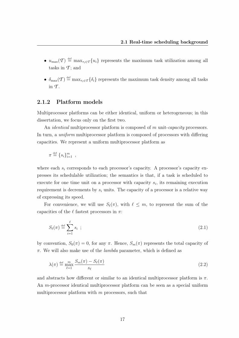
Multiprocessor platforms can be either identical, uniform or heterogeneous; in thisdissertation, we focus only on the first two.

An identical multiprocessor platform is composed of m unit-capacity processors.In turn, a uniform multiprocessor platform is composed of processors with differingcapacities. We represent a uniform multiprocessor platform as

πdef= {si}mi=1 ,

where each si corresponds to each processor’s capacity. A processor’s capacity ex-presses its schedulable utilization; the semantics is that, if a task is scheduled toexecute for one time unit on a processor with capacity si, its remaining executionrequirement is decrements by si units. The capacity of a processor is a relative wayof expressing its speed.

For convenience, we will use S`(π), with ` ≤ m, to represent the sum of thecapacities of the ` fastest processors in π:

S`(π)def=∑i=1

si ; (2.1)

by convention, S0(π) = 0, for any π. Hence, Sm(π) represents the total capacity ofπ. We will also make use of the lambda parameter, which is defined as

λ(π)def=

mmax`=1

Sm(π)− S`(π)

s`(2.2)

and abstracts how different or similar to an identical multiprocessor platform is π.An m-processor identical multiprocessor platform can be seen as a special uniformmultiprocessor platform with m processors, such that

17

2. Background and Related Work

• si = 1.0, for all 1 ≤ i ≤ m;

• S`(π) = `, for all 0 ≤ i ≤ m; and

• λ(π) = m− 1.

2.1.3 Scheduling algorithm classification

In this dissertation, we focus on preemptive priority-driven scheduling algorithms.They work by assigning priorities to the active jobs, and selecting that (or those)with highest priority for execution. Since we deal with preemptive algorithms, a jobis forced to suspend its execution (i.e., is preempted) if one or more higher priorityjobs justifies it. To survey scheduling algorithms and schedulability analysis results,scheduling algorithms can be classified according to how priorities are assigned tojobs and, for multiprocessor, according to how jobs may be scheduled on the availableprocessors.

2.1.3.1 Priority-based classification

Regarding priority assignment, we divide algorithms into three categories: fixed taskpriority, fixed job priority, and dynamic priority. This taxonomy is widely used inthe literature, although the specific names of the categories vary (Davis & Burns,2011).3

With fixed task priority, priority is a characteristic of the task. Therefore, all ofa task’s jobs are applied the same priority. Whenever two tasks have active jobs,the relationship between those two jobs’ priorities will always be the same.

With fixed job priority, priority is a characteristic of the job. The jobs of eachtask may have different priorities, but each job has always the same priority sinceit becomes active until it finishes execution.

Finally, with dynamic priority, priority is a characteristic of the job which maychange over time.

3In uniprocessor scheduling, due to some optimality results (Section 2.1.4.1), it is also commonto merge the fixed job priority and dynamic priority algorithms (thus having a 2-category taxonomyof fixed vs. dynamic priority algorithms) (Carpenter et al., 2004).

18

2.1 Real-time scheduling background

2.1.3.2 Migration-based classification

Regarding the degree of migration allowed when allocating the workload amongthe available processors, algorithms for multiprocessors can be categorized as eitherpartitioned (no migration), restricted-migration global (task-level migration only)or unrestricted-migration global (full job-level migration).

In partitioned algorithms, tasks are assigned to processors and all of each task’sjobs execute on the same processor. The scheduler maintains a separate job queuefor each processor, and reduces the problem of scheduling to multiple instances ofuniprocessor scheduling.

In restricted-migration global algorithms, the jobs of one same task may executeon different processor throughout time, but each job will always execute on the sameprocessor. Conversely, in unrestricted-migration global algorithms, any job may bepreempted in one processor and resume execution in another processor. Withoutloss of generality, we follow the assumption (common in real-time scheduling theory)that the cost of a job’s migration from one processor to another is either negligibleor already accounted for in its execution requirement. For this reason, regardingglobal multiprocessor scheduling, we will only consider unrestricted-migration globalscheduling algorithms, to which we will refer to as simply “global”.

2.1.3.3 Work-conserving algorithms

A scheduling algorithm is said to be work-conserving if it guarantees that thereexists no instant at which some processing capacity is unused (idle) and there is anactive job (ready to execute).

2.1.4 Schedulability analysis notions

2.1.4.1 Feasibility, schedulability, and optimality

A task set T is feasible if and only if there exists a sequence S according to which alljobs of all tasks τi ∈ T fulfill their timeliness requirements. Regarding schedulability,let A be a scheduling algorithm. A task set T is A-schedulable if and only if, whenscheduled according to algorithm A, all jobs of all tasks τi ∈ T fulfill their timelinessrequirements.

19

2. Background and Related Work

Furthermore algorithm A is said to be optimal, within some class of algorithmsto which it belongs and some task model which it is able to schedule, if every taskset (obeying to such task model) which is schedulable according to some algorithmin that class is also A-schedulable. For example, the Deadline Monotonic schedulingalgorithm is an optimal algorithm w.r.t. uniprocessor fixed task priority schedulingof constrained-deadline sporadic task sets.

2.1.4.2 Types of tests

As in logic in general, there are three types of tests in schedulability analysis: suffi-cient, necessary and exact (sufficient and necessary). With a sufficient schedulabilitytest, we are able to assess if a task set is schedulable under given assumptions, butwe are not able to asses if a task set is not schedulable— if the test does not give apositive result, the result is inconclusive and we can only say that the task set maybe unschedulable. With an exact (necessary and sufficient) schedulability test wecan surely assess if a task set is schedulable or not under given assumptions. Thesame applies for sufficient/exact feasibility tests.

2.2 Hard real-time scheduling on dedicated plat-forms

2.2.1 Scheduling on uniprocessor platforms

Scheduling is assumed to occur on a unit-capacity processor. This means that,within each unit of time, one unit of the execution requirement of the scheduledjob is executed— in other terms, each processor has a schedulable utilization of oneexecution unit per time unit.

2.2.1.1 Fixed task priority

The seminal example of an algorithm using a fixed task priorities assignment is RateMonotonic (RM), proposed by Liu & Layland (1973), in which higher priorities areassigned to tasks with shorter periods. RM assumes an implicit-deadline periodic

20

2.2 Hard real-time scheduling on dedicated platforms

task model. In a classical result, Liu & Layland (1973)’s sufficient test states that a

periodic task set T is RM-schedulable on a unit-speed processor if

usum(T ) ≤ n(21/n − 1) .

Sufficient tests subsequently proposed by Lauzac et al. (1998) and by Bini et al.

(2003) have been found to outperform it (Lupu et al., 2010). Exact schedulability

of implicit-deadline periodic tasks can be assessed through response time analysis

(Audsley et al., 1993).

Leung & Whitehead (1982) extended Liu & Layland (1973)’s analysis to the

case of constrained deadlines, proposing the Deadline Monotonic algorithm, which

assigns higher priorities to tasks in non-increasing order of their (relative) deadlines.

Lehoczky (1990) in turn extended Leung & Whitehead (1982)’s analysis on the

Deadline Monotonic scheduling to periodic task sets with arbitrary deadlines.

2.2.1.2 Fixed job priority

The Earliest Deadline First (EDF) algorithm (Liu & Layland, 1973) is the lead

member of this category; in EDF, jobs are prioritized according to their absolute

deadline time, which is constant. An implicit-deadline periodic task set T is EDF-

schedulable on a unit-speed processor if and only if (Liu & Layland, 1973)

usum ≤ 1 . (2.3)

Dertouzos (1974) proved that EDF is optimal for the uniprocessor. This result

is obtained by proving that any feasible schedule can be transformed into a schedule

which follows the EDF strategy (Dertouzos & Mok, 1989).

For constrained-deadline sporadic task sets, the condition in Equation (2.3) is

only sufficient. Baruah et al. (1990) proved an exact (sufficient and necessary)

condition, incorporating the notion of demand bound function, which provides an

upper bound on the maximum cumulative execution requirement by jobs of sporadic

task τi which have both their arrival and deadline times within any time interval

21

2. Background and Related Work

with length t. For EDF scheduling, it is defined as

dbf(τi, t)def= max

{0,

(⌊t−Di

Ti+ 1

⌋)·Ci}

. (2.4)

They have derived the following exact condition based on the demand bound func-tion: a constrained-deadline sporadic task set T is EDF-schedulable on a unit-speedprocessor if and only if usum ≤ 1 (Equation (2.3)) and∑

τi∈T

dbf(τi, t) ≤ t, for all t > 0 . (2.5)

The demand bound function is used to compute the load function of a sporadictask system:

load(T )def= max

t>0

∑τi∈T dbf(τi, t)

t. (2.6)

Using this function, the condition expressed in Equation (2.5) can be expressed asload(T ) ≤ 1. The load function is also used in multiprocessor schedulability tests,as we see in forthcoming sections.

2.2.1.3 Dynamic priority

An example of an algorithm with such priority assignment is Least Laxity First(LLF), which assigns priority according to each job’s laxity (Mok, 1983)—which isthe difference between the remaining time until its absolute deadline time and totaltime the job needs to be allowed to execute to finish its execution requirement.

LLF is found to be optimal for the uniprocessor case. According to Dertouzos& Mok (1989), such optimality can be proved in the same way as Dertouzos (1974)proves the optimality of EDF.

2.2.2 Partitioned scheduling on identical multiprocessors

Partitioned scheduling can be seen as consisting of two steps: partitioning tasksamong processors (offline), and scheduling the tasks assigned to each processor usingan uniprocessor algorithm (online) (Baker & Baruah, 2007).

22

2.2 Hard real-time scheduling on dedicated platforms

Dhall & Liu (1978) described a phenomenon which remained known as “Dhalleffect”, which we describe in detail in Section 2.2.3.1, and which established for someyears a generalized perception of superiority of partitioned scheduling over globalscheduling.

Nevertheless, partitioning scheduling lends itself to non-work-conserving behav-ior; tasks with active jobs will not take advantage of idle capacity of processorsother than the one to which the task is assigned. As such, we focus on globalmultiprocessor scheduling.

Partitioning tasks into processors is equivalent to a bin-packing problem, which isproven to be NP-hard in the strong sense. For this reason, heuristic-based strategiesare employed to make the problem tractable. Such strategies are characterized bytwo aspects: in which order as the tasks considered (the task sorting criterion),and how is processor for each task selected (the heuristic itself). The possible tasksorting criteria come from the set:

{Increasing,Decreasing} × {Di, δi, Ti, ui} .

After chosing a task sorting criterion, each task in order is assigned to a processor,employing one of the following heuristics:

• First Fit—select the first processor where the task fits (starting from the veryfirst);

• Next Fit—select the first processor where the task fits (starting from current);

• Best Fit—select the processor where the task fits with less remaining processorcapacity;

• Worst Fit—select the processor where task fits with most remaining processorcapacity.

Verification of whether a task fits on a processor is done using uniprocessor schedu-lability tests.

According to Lupu et al. (2010), the choice of strategy depends on the total den-sity of the task set, and on whether the goal is to minimize the number of processors

23

2. Background and Related Work

or to ensure that processors have some slack to accommodate, for instance, the ad-mission of new tasks in runtime. The Decreasing δi sorting criterion is suitable formost cases (independently of the employed schedulability test). Regarding heuris-tics, if the goal is to minimize m, then Next Fit or Best Fit are preferred (dependingon whether the total density of the task set is, respectively, ≤ 0.5 ·m or > 0.5 ·m);if the goal is to ensure execution slack, Worst Fit is preferred.

2.2.3 Global scheduling on identical multiprocessors

Global scheduling algorithms on identical multiprocessors are, by construction, work-conserving, since:

1. if there is an active job waiting to execute, no processor is idle; and

2. when the number of active jobs is less than the number of processors, all activejobs are executing.

This does not, however, make them superior to their partitioned counterparts, aswe now see.

2.2.3.1 Fixed job priority

As mentioned, fixed job priority global scheduling is subject to the so-called “Dhalleffect” (Dhall & Liu, 1978): some task sets with arbitrarily low total utilizations canbe unschedulable regardless of the number of processors employed. The prototypicalscenario of the “Dhall effect” (characterized by one high utilization task and severalhigher-priority low utilization tasks) can be solved using partitioned scheduling (toeliminate the contention between the high and low utilization tasks). This led toa perceived superiority of partitioned scheduling, which had impact of the focusof forthcoming real-time scheduling research. Such superiority was eventually dis-proved. Leung & Whitehead (1982) showed that there are some sporadic task setswhich are scheduled by some partitioned fixed task priority algorithm but not byany global fixed task priority algorithm, as well as some sporadic task sets which arescheduled by some global fixed task priority algorithm but not by any partitionedfixed task priority algorithm. More succinctly, this result proves that global and

24

2.2 Hard real-time scheduling on dedicated platforms

partitioned scheduling are incomparable with respect to fixed task priority schedul-ing algorithms. Baruah (2007) proved that global and partitioned scheduling areincomparable with regard to fixed job priority as well.

In the realm of global multiprocessor scheduling, fixed job priority algorithmssuch as EDF have received more attention than fixed task priority ones (Baker &Baruah, 2007). Buttazzo (2005) performed comparative experiments between RMand EDF, and point out that the real advantage of RM over EDF is implementationsimplicity. In turn, EDF allows a more efficient utilization of the processor, whichthe authors point out has particular advantage when dealing with embedded systemsand resource reservations (a particular case of hierarchical scheduling). Hence, inthis dissertation, we focus mostly on global EDF (gEDF).

Goossens et al. (2003) studied gEDF scheduling of implicit-deadline sporadictask sets, providing a sufficient gEDF-schedulability test. Minor extensions to theirproofs yield the so-called “density test” (Baruah, 2007) for constrained-deadline pe-riodic task sets. According to this test, task set T is gEDF-schedulable on anm-processor identical multiprocessor platform if

δsum(T ) ≤ m− (m− 1) · δmax(T ) .

Baker (2003) proposed a sufficient gEDF-schedulability test for constrained-deadline periodic task sets on an m-processor identical multiprocessor platform.Before the test itself, we now highlight the structure of the proof by contrapositivedeveloped by Baker (2003), which was used in several later works on schedulabilityof sporadic task sets.

1. Assume some job of a task τk ∈ T misses its deadline at instant td (and it isthe first job to miss a deadline).

2. Consider an interval [t0, td[ (with t0 < td), which is dubbed the interferenceinterval. The exact definition of t0 differs among works employing this proofstructure.

3. Obtain an upper bound on the amount of work that gEDF is required (butfails) to over the interval [t0, td[. Two sources contribute to this interference:

25

2. Background and Related Work

timeti t0 ta td

Di

φi Ak Dk

τi τk

deadline miss

Figure 2.1: Execution pattern considered in Baker (2003)’s proof and thereon inspired works.

(i) jobs released in the interval; and (ii) jobs released before ta which have

not completed their execution up to that instant (carry-in jobs).

4. Derive a necessary condition for unschedulability—which will have the form

“If task set T is not gEDF-schedulable, then, for some task τk ∈ T , condition

ψ holds”.

5. Take the contrapositive of this condition (“task set T is gEDF-schedulable if,

for all tasks τk ∈ T , condition ψ does not hold”), which yields a sufficient

condition for schedulability.

The execution pattern underlying to this proof structure is shown in Figure 2.1.

Besides the considered job of task τk, the figure illustrates a hypothetical job of task

τi which is released prior to time instant t0 and carries in some execution to the

considered interference interval, [t0, td[.

To derive their sufficient gEDF-schedulability tests, Baker (2003) considers t0to be the earliest time instant prior to the arrival of the deadline-missing job of τk(ta = td − Dk) at which a certain condition is satisfied, whereas Bertogna et al.

(2005) considered t0 = ta = td − Dk. Baruah (2007) analyzed the shortcomings

of both Baker (2003)’s and Bertogna et al. (2005)’s tests, and derived a sufficient

schedulability test by employing Baker (2003)’s strategy, considering t0 to be the

earliest time instant prior to the arrival of the deadline-missing job of τk at which

some processor is idle. As pointed out before, since gEDF is a work-conserving

scheduling algorithm, if some processor is idle, then all the active jobs must be

executing on some processor. The sufficient schedulability condition obtained by

26

2.2 Hard real-time scheduling on dedicated platforms

Baruah (2007) is that, for all tasks τk ∈ T and for all Ak ≥ 0,

∑τi∈T

Ii +∑

m−1 largest

(Ii − Ii) ≤ m(Ak +Dk − Ck) ,

where

Iidef=

{min{dbf(τi, Ak +Dk)− Ck, Ak} if i = k

min{dbf(τi, Ak +Dk), Ak +Dk − Ck} otherwise, (2.7)

Iidef=

{min{dbf′(τi, Ak +Dk)− Ck, Ak} if i = k

min{dbf′(τi, Ak +Dk), Ak +Dk − Ck} otherwise, and

dbf′(τi, t)def=

⌊t

Ti

⌋·Ci + min

{Ci, t−

⌈t+ Ti −Di

Ti

⌉·Ti}

.

Ii and Ii are upper bounds on the interference of τi, respectively if it does or does

not have a job carrying in some execution to the [t0, td[ time interval. By definition

of the interval, at most m− 1 tasks have such carry-in jobs.

2.2.3.2 Hybrid variants of gEDF

To address the previously described “Dhall effect” (Dhall & Liu, 1978) without being

subject to the higher number of preemptions characteristic of LLF, hybrid variants

of gEDF were developed. EDZL (Earliest Deadline until Zero Laxity) (Lee, 1994)

borrows the use of laxity from LLF, but only considers it for priority assignment pur-

poses when needed. EDZL gives highest priority to jobs with zero laxity, assigning

the priorities of the remaining jobs according to the classic EDF policy.

Other approaches involve applying fixed priorities to some tasks, while maintain-

ing the fixed job priority aspect of EDF for the remaining tasks. EDF-US (Srinivasan

& Baruah, 2002) gives a static highest priority to tasks with utilizations greater thanm

2m−1(with ties arbitrarily broken), and schedules the remaining tasks’ jobs accord-

ing to the classic EDF policy. fpEDF (Baruah, 2004) gives a static highest priority

to at most m− 1 tasks with utilization greater than 12, and schedules the remaining

tasks’ jobs according to the classic EDF policy.

27

2. Background and Related Work

2.2.4 Global scheduling on uniform multiprocessors

We already saw that global scheduling algorithms on identical multiprocessors are,by construction, work-conserving. The same does not automatically apply for uni-form multiprocessors without specific considerations. Funk et al. (2001) introduceda gEDF scheduling strategy which is work-conserving on uniform multiprocessors.Such property is achieved by obeying to the following rules (cf. rules for globalscheduling on identical multiprocessors, Section 2.2.3):

1. if there is an active job waiting to execute, no processor is idle;

2. when the number of active jobs is less than the number of processors, the jobsexecute on the fastest processors (and only the slowest ones are idle); and

3. higher-priority (in the case of gEDF, earlier-deadline) jobs execute on fasterprocessors.

Baruah & Goossens (2008) provide a sufficient gEDF-schedulability test for con-strained-deadline sporadic task sets on uniform multiprocessors. They derive itusing Baker (2003)’s technique: from an execution pattern where a job is the firstto miss a deadline, they derive a necessary unschedulability condition; then, thecontrapositive of this condition provides a sufficient condition for schedulability. Inderiving the necessary unschedulability condition, Baruah & Goossens (2008) takespecial advantage of the second aforementioned rule of gEDF— if some processor isidle, then an active job is guaranteed to be executing on a processor at least as fastas that one. The authors thus prove that task set T is schedulable by gEDF on anm-processors uniform multiprocessor platform π if

load(T ) ≤ Sm(π)− (λ(π)− ν) · δmax(T ) , (2.8)

where load(T ) is defined as seen in Equation (2.6), and

νdef= max {` : S`(π) < Sm(π)− λ(π) · δmax(T )} . (2.9)

We refer back to this test in Chapter 4, since we extend Baruah & Goossens (2008)’sreasoning to the case when the uniform multiprocessor platform is not totally avail-able at all times.

28

2.3 Scheduling approaches for mixed systems

2.3 Scheduling approaches for mixed systems

In the previous section, we have seen related work focused on system models whereone scheduler has to guarantee the HRT requirements of periodic or sporadic tasks.We now look into approaches which have been proposed in the literature to deal withsystems that encompass tasks with mixed criticality, real-time requirements (HRT,SRT, non-real-time), activation models (periodic, sporadic, aperiodic), and/or origin(various development teams or providers).4

2.3.1 Resource reservation frameworks

In some domains of application, systems may have two coexisting types of workload:

1. a hard real-time (HRT) workload, whose temporal characteristics are knownbeforehand and which has strict deadlines; and

2. an aperiodic workload, whose temporal characteristics (e.g., execution require-ment) may not be known beforehand, and which can have SRT or non-real-timerequirements.

An efficient scheduling approach for such a system shall guarantee the fulfillmentof the HRT tasks’ deadlines and maximize the quality of service (QoS) of the SRTtasks (without compromising the former). There are several ways of characterizingthe QoS of SRT tasks— for instance, average response time.

The simplest way of guaranteeing temporal isolation of HRT tasks is by relegatingSRT and non-real-time tasks to the lowest priority, causing them to be scheduledonly when there are no HRT tasks ready to execute. However, this leads to longresponse times for the SRT and non-real-time tasks; in the case of SRT tasks, this isincompatible with our goal of providing some QoS guarantee. This issue is addressedby employing resource reservations; the term was introduced by Mercer et al. (1993).Figure 2.2 shows an example resource reservation framework. Under this approach,fractions of the processor availability are reserved to a certain task or subset of tasks.

4Although we deal with models for mixed criticality systems, the paradigm of mixed criticality(or multi-criticality) scheduling proposed by Vestal (2007) is beyond the scope of this dissertation.

29

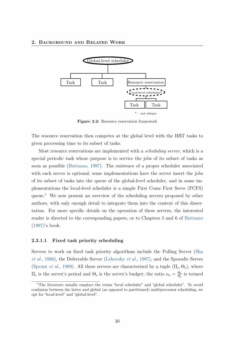
2. Background and Related Work

Global-level scheduler

Local-level scheduler*

Task Task

Task Task

Resource reservation

* – not always

Figure 2.2: Resource reservation framework

The resource reservation then competes at the global level with the HRT tasks togiven processing time to its subset of tasks.

Most resource reservations are implemented with a scheduling server, which is aspecial periodic task whose purpose is to service the jobs of its subset of tasks assoon as possible (Buttazzo, 1997). The existence of a proper scheduler associatedwith each server is optional; some implementations have the server insert the jobsof its subset of tasks into the queue of the global-level scheduler, and in some im-plementations the local-level scheduler is a simple First Come First Serve (FCFS)queue.5 We now present an overview of the scheduling servers proposed by otherauthors, with only enough detail to integrate them into the context of this disser-tation. For more specific details on the operation of these servers, the interestedreader is directed to the corresponding papers, or to Chapters 5 and 6 of Buttazzo(1997)’s book.

2.3.1.1 Fixed task priority scheduling

Servers to work on fixed task priority algorithms include the Polling Server (Shaet al., 1986), the Deferrable Server (Lehoczky et al., 1987), and the Sporadic Server(Sprunt et al., 1989). All these servers are characterized by a tuple (Πs,Θs), whereΠs is the server’s period and Θs is the server’s budget; the ratio αs = Θs

Πsis termed

5The literature usually employs the terms “local scheduler” and “global scheduler”. To avoidconfusion between the latter and global (as opposed to partitioned) multiprocessor scheduling, weopt for “local-level” and “global-level”.

30

2.3 Scheduling approaches for mixed systems

the server’s bandwidth. The server is scheduled as a highest priority periodic task τiwith period Ti = Πs and execution requirement Ci = Θs.

2.3.1.2 Fixed job priority scheduling

To work with fixed job priority algorithms (such as EDF), Spuri & Buttazzo (1994)propose several server mechanisms, of which we highlight two. The Dynamic Spo-radic Server is an extension of the Sporadic Server whereby the priority of theserver is based on a deadline value, which is updated each time the server’s budgetis replenished. The Total Bandwidth Server is markedly different, in the followingaspects:

• the Total Bandwidth Server is not characterized by a (Πs,Θs) tuple, but onlyby a bandwidth αs;

• instead of being scheduled to provide its budget to the jobs of SRT aperiodictasks, the Total Bandwidth Server assigns deadlines to the latter and insertsthem into the same queue as the jobs of HRT tasks, to be scheduled by EDF.

However, the Total Bandwidth Server is also subject to classical task schedulabilityanalysis as the other servers. To assess the schedulability of the system composed ofHRT tasks and one Total Bandwidth Server, the latter is considered as equivalentto a task with utilization ui = αs. Abeni & Buttazzo (1998) propose the ConstantBandwidth Server (CBS), in a scheme with one server to handle each SRT task. Thisscheme guarantees temporal isolation between HRT and SRT tasks, and among eachof the latter.

Baruah et al. (2002) present M-CBS, an extension of the CBS scheme for mul-tiprocessors. For the purpose of this literature review, the main difference to behighlighted is that M-CBS employs, instead of EDF, a scheduling strategy basedon the contemporarily proposed EDF-US (Srinivasan & Baruah, 2002): a subset ofservers with highest utilization are considered high-priority servers (with their pri-ority ties broken arbitrarily but consistently), whereas the remaining are considereddeadline-based servers (and are scheduled according to EDF).

31

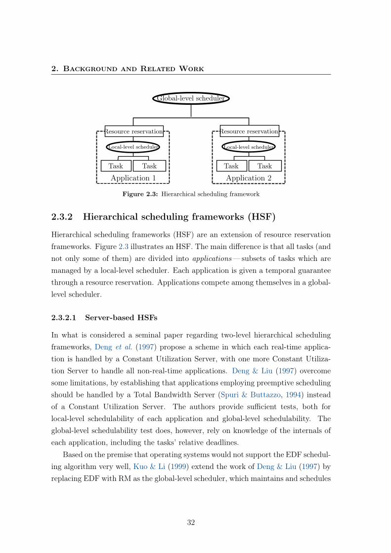
2. Background and Related Work

Global-level scheduler

Local-level scheduler Local-level scheduler

Task Task Task Task

Application 1 Application 2

Resource reservation Resource reservation

Figure 2.3: Hierarchical scheduling framework

2.3.2 Hierarchical scheduling frameworks (HSF)

Hierarchical scheduling frameworks (HSF) are an extension of resource reservationframeworks. Figure 2.3 illustrates an HSF. The main difference is that all tasks (andnot only some of them) are divided into applications—subsets of tasks which aremanaged by a local-level scheduler. Each application is given a temporal guaranteethrough a resource reservation. Applications compete among themselves in a global-level scheduler.

2.3.2.1 Server-based HSFs

In what is considered a seminal paper regarding two-level hierarchical schedulingframeworks, Deng et al. (1997) propose a scheme in which each real-time applica-tion is handled by a Constant Utilization Server, with one more Constant Utiliza-tion Server to handle all non-real-time applications. Deng & Liu (1997) overcomesome limitations, by establishing that applications employing preemptive schedulingshould be handled by a Total Bandwidth Server (Spuri & Buttazzo, 1994) insteadof a Constant Utilization Server. The authors provide sufficient tests, both forlocal-level schedulability of each application and global-level schedulability. Theglobal-level schedulability test does, however, rely on knowledge of the internals ofeach application, including the tasks’ relative deadlines.

Based on the premise that operating systems would not support the EDF schedul-ing algorithm very well, Kuo & Li (1999) extend the work of Deng & Liu (1997) byreplacing EDF with RM as the global-level scheduler, which maintains and schedules

32

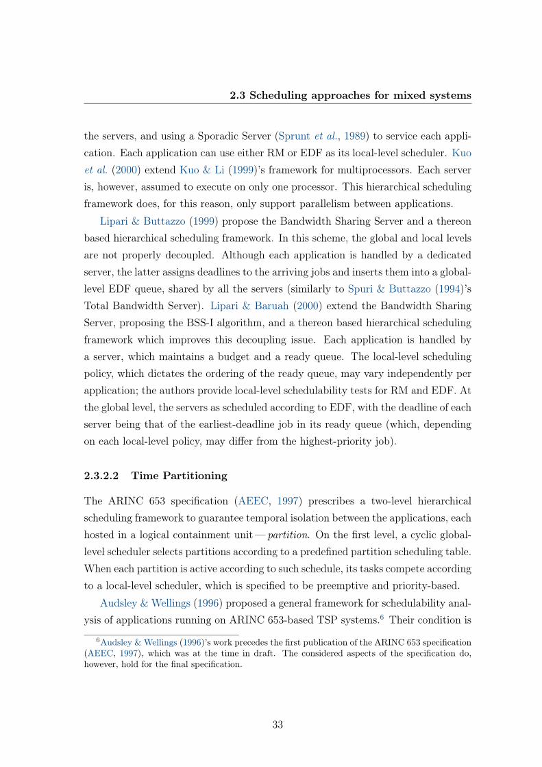
2.3 Scheduling approaches for mixed systems

the servers, and using a Sporadic Server (Sprunt et al., 1989) to service each appli-cation. Each application can use either RM or EDF as its local-level scheduler. Kuoet al. (2000) extend Kuo & Li (1999)’s framework for multiprocessors. Each serveris, however, assumed to execute on only one processor. This hierarchical schedulingframework does, for this reason, only support parallelism between applications.

Lipari & Buttazzo (1999) propose the Bandwidth Sharing Server and a thereonbased hierarchical scheduling framework. In this scheme, the global and local levelsare not properly decoupled. Although each application is handled by a dedicatedserver, the latter assigns deadlines to the arriving jobs and inserts them into a global-level EDF queue, shared by all the servers (similarly to Spuri & Buttazzo (1994)’sTotal Bandwidth Server). Lipari & Baruah (2000) extend the Bandwidth SharingServer, proposing the BSS-I algorithm, and a thereon based hierarchical schedulingframework which improves this decoupling issue. Each application is handled bya server, which maintains a budget and a ready queue. The local-level schedulingpolicy, which dictates the ordering of the ready queue, may vary independently perapplication; the authors provide local-level schedulability tests for RM and EDF. Atthe global level, the servers as scheduled according to EDF, with the deadline of eachserver being that of the earliest-deadline job in its ready queue (which, dependingon each local-level policy, may differ from the highest-priority job).

2.3.2.2 Time Partitioning

The ARINC 653 specification (AEEC, 1997) prescribes a two-level hierarchicalscheduling framework to guarantee temporal isolation between the applications, eachhosted in a logical containment unit— partition. On the first level, a cyclic global-level scheduler selects partitions according to a predefined partition scheduling table.When each partition is active according to such schedule, its tasks compete accordingto a local-level scheduler, which is specified to be preemptive and priority-based.

Audsley & Wellings (1996) proposed a general framework for schedulability anal-ysis of applications running on ARINC 653-based TSP systems.6 Their condition is

6Audsley & Wellings (1996)’s work precedes the first publication of the ARINC 653 specification(AEEC, 1997), which was at the time in draft. The considered aspects of the specification do,however, hold for the final specification.

33

2. Background and Related Work

based on response time analysis, and assumes the knowledge of (besides each task’stiming characteristics as per the sporadic task model):

• the worst-case blocking time each task may be subject to by lower-prioritytasks in the same partition;

• the worst-case delay each partition may experience as a consequence of theoperating system entering a critical section;

• the worst-case delay between an event occurring and the corresponding taskbeing placed into the scheduler’s ready queue; and

• the maximum overhead that the operating system can cause within a certaintime interval (as a consequence of interrupt service routines, context switching,etc.).

Some of these parameters cause the schedulability analysis of one application (par-tition) to depend on knowing characteristics of applications running in other parti-tions and the exact partition scheduling table. For this reason, Audsley & Wellings(1996)’s framework does not allow a usable independent analysis of each application,neither the computation of a partition schedule to guarantee schedulability.

Lee et al. (1998) proposed a sufficient test to assess the schedulability of anapplication (contained in a partition) composed of a task set scheduled according tosome fixed task priority policy. Their test depends on the knowledge of the periodaccording to which the partition is scheduled and of the fraction of this periodduring which the partition is scheduled—the bandwidth (cf. server bandwidth,Section 2.3.1). For the test to produce a conclusive positive result, two conditionsmust hold:

• the task set is schedulable—according to Lehoczky (1990)’s test—on a slowerdedicated processor (whose speed corresponds to the partition’s bandwidth);and

• the period according to which the partition is scheduled does not exceed abound, calculated as a function of the bandwidth and the timing characteristicsof the task set.

34

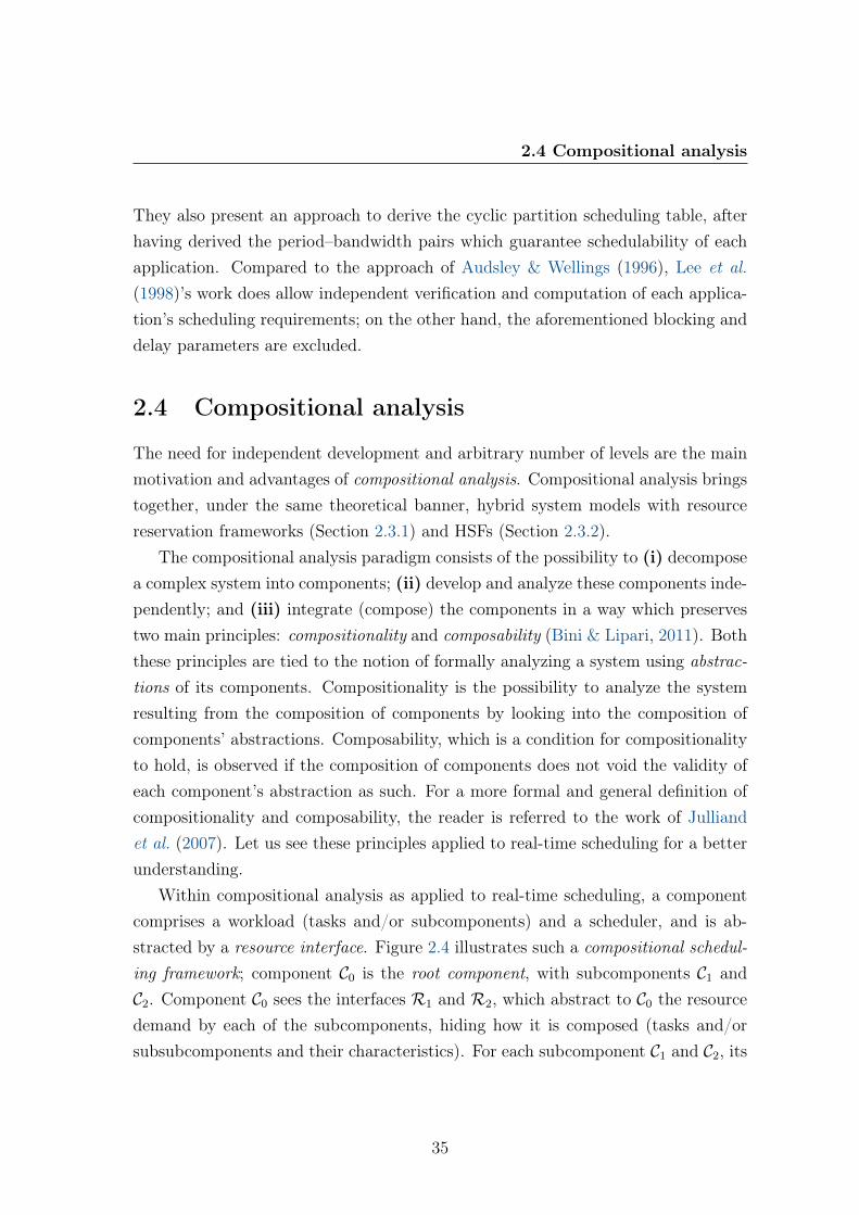
2.4 Compositional analysis

They also present an approach to derive the cyclic partition scheduling table, afterhaving derived the period–bandwidth pairs which guarantee schedulability of eachapplication. Compared to the approach of Audsley & Wellings (1996), Lee et al.(1998)’s work does allow independent verification and computation of each applica-tion’s scheduling requirements; on the other hand, the aforementioned blocking anddelay parameters are excluded.

2.4 Compositional analysis

The need for independent development and arbitrary number of levels are the mainmotivation and advantages of compositional analysis. Compositional analysis bringstogether, under the same theoretical banner, hybrid system models with resourcereservation frameworks (Section 2.3.1) and HSFs (Section 2.3.2).

The compositional analysis paradigm consists of the possibility to (i) decomposea complex system into components; (ii) develop and analyze these components inde-pendently; and (iii) integrate (compose) the components in a way which preservestwo main principles: compositionality and composability (Bini & Lipari, 2011). Boththese principles are tied to the notion of formally analyzing a system using abstrac-tions of its components. Compositionality is the possibility to analyze the systemresulting from the composition of components by looking into the composition ofcomponents’ abstractions. Composability, which is a condition for compositionalityto hold, is observed if the composition of components does not void the validity ofeach component’s abstraction as such. For a more formal and general definition ofcompositionality and composability, the reader is referred to the work of Julliandet al. (2007). Let us see these principles applied to real-time scheduling for a betterunderstanding.

Within compositional analysis as applied to real-time scheduling, a componentcomprises a workload (tasks and/or subcomponents) and a scheduler, and is ab-stracted by a resource interface. Figure 2.4 illustrates such a compositional schedul-ing framework; component C0 is the root component, with subcomponents C1 andC2. Component C0 sees the interfaces R1 and R2, which abstract to C0 the resourcedemand by each of the subcomponents, hiding how it is composed (tasks and/orsubsubcomponents and their characteristics). For each subcomponent C1 and C2, its

35

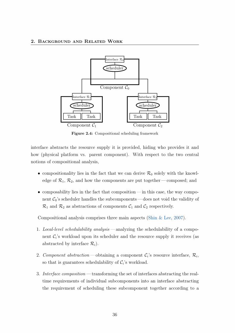
2. Background and Related Work

scheduler

Interface R0

scheduler scheduler

Task Task Task Task

Component C0

Component C1 Component C2

Interface R2Interface R1

Figure 2.4: Compositional scheduling framework

interface abstracts the resource supply it is provided, hiding who provides it andhow (physical platform vs. parent component). With respect to the two centralnotions of compositional analysis,

• compositionality lies in the fact that we can derive R0 solely with the knowl-edge of R1, R2, and how the components are put together—composed; and

• composability lies in the fact that composition— in this case, the way compo-nent C0’s scheduler handles the subcomponents—does not void the validity ofR1 and R2 as abstractions of components C1 and C2 respectively.

Compositional analysis comprises three main aspects (Shin & Lee, 2007).

1. Local-level schedulability analysis—analyzing the schedulability of a compo-nent Ci’s workload upon its scheduler and the resource supply it receives (asabstracted by interface Ri).

2. Component abstraction—obtaining a component Ci’s resource interface, Ri,so that is guarantees schedulability of Ci’s workload.

3. Interface composition—transforming the set of interfaces abstracting the real-time requirements of individual subcomponents into an interface abstractingthe requirement of scheduling these subcomponent together according to a

36

2.4 Compositional analysis

given intercomponent scheduling strategy. Formally, given a set of interfacesR1, R2, . . . , derive an interface R0 which is compatible with R1‖R2‖ . . .(where the composition operator, ‖, models the intercomponent schedulingstrategy). Observing composability and compositionality, we can say that R0

is compatible with C0 (i.e., C1‖C2‖ . . .).

In this section, we survey, under the light of these three aspects, the work that hasbeen done in compositional analysis. First, let us introduce some additional notionsand definitions which are common to all or most approaches thereto.

2.4.1 Common definitions

Mok et al. (2001) introduce, to support their static partition and bounded-delayresource models (which we review later on), some concepts which are common tosubsequent works in the field. We now present those concepts, updating their ter-minology and notation to reflect present widespread use. For this purpose, we firstintroduce a function supply(R, t1, t2), as expressing the effective supply that isprovided according to interface R over the time interval [t1, t2[. For some resourcemodels, as we will see ahead, the exact knowledge of the effective supply is notfeasible.

The supply bound function sbf(R, t) gives the minimum resource supply guaran-teed by interface R over any interval of length t. Its main property is, consequently,that

sbf(R, t) ≤ mino≥0

supply(R, o, o+ t) . (2.10)

Since the supply bound function may be a step function (rather than a linear one),some authors also make use of a linear lower bound on the supply bound function.The characterizing property of this function is that

lsbf(R, t) ≤ sbf(R, t), for all t > 0 .

The resource bandwidth α (cf. server bandwidth, Section 2.3.1) represents the

37

2. Background and Related Work

fraction of resource that is provided over time. Formally, it is defined as follows:

αdef= lim

t→+∞

supply(R, 0, t)t

. (2.11)

The resource models we consider, being periodic in nature (at least to some extent),allow computing bandwidth in a way which is significantly less complex than theformal definition.

2.4.2 Uniprocessor

2.4.2.1 Static partition resource model

Mok et al. (2001) introduce a static partition resource model as an abstraction of aresource which is made available to a group of tasks only during specific intervals.This models very closely the resource supply mechanism present in ARINC 653TSP systems (Section 2.3.2.2). A resource partition P is defined as a tuple (ω,Π),with ω = {(Si, Ei)}Ni=1 and Π being the period of the partition. Each pair (Si, Ei)

represents a time window (respectively, its start and end) in terms of offset relativeto the beginning of each period of length Π. Formally, this means that the processoris available to the task set executing on this partition only during the time intervals:

[k · Π + Si; k · Π + Ei[, for all i ∈ [1..N ], and for all k ∈ N0 .

Since the allocation defined in ω repeats over a period of length Π, the bandwidthis calculated simply as

α =

∑(Si,Ei)∈ω(Ei − Si)

Π.

The computation of supply(P , t1, t2) is straightforward, and the definition ofa supply bound function fulfilling the formal definition in Equation (2.10) followsdirectly: sbf(P , t) def

= mino≥0 supply(R, o, o+ t) for all t > 0. The authors do not,however, present a means to compute it.

Local-level schedulability analysis Mok et al. (2001) show that the optimalityof EDF on uniprocessor also holds for the static partition resource model; this means

38

2.4 Compositional analysis

that any task set that is feasible on a static partition P is also EDF-schedulable onP . From there, an exact EDF-schedulability test for implicit-deadline periodic tasksets on a static partition is derived. Periodic task set T is schedulable with EDFon a static partition P if and only if∑

τi∈T

dbf(τi, t) ≤ sbf(P , t), for all t > 0 .

Component abstraction / Interface composition Mok et al. (2001) pointout that the static partition resource model is more adequate for scenarios wherethe resource (the processor) is already partitioned. For this reason, the authors donot approach component abstraction (and, consequently, interface composition) andpropose a more appropriate model: the bounded-delay resource model.

2.4.2.2 Bounded-delay resource model

The bounded-delay resource model (Mok et al., 2001) consists of a tuple Φdef= (α,∆),

where α is the bandwidth (as per Equation (2.11)) and ∆ is the delay bound—themaximum delay in the partition’s resource supply, in relation to what it would receivewhen executing on a fully available processor with speed α (instead of a partiallyavailable processor of speed 1); the authors call this slower processor scenario thenormalized execution of Φ. This is similar to the reasoning done by Lee et al. (1998),of confronting execution on a shared resource and execution on a slower resource.

Shin & Lee (2004) build upon Mok et al. (2001)’s work, introducing a com-positional scheduling framework based on the bounded-delay resource model. Thedefinition of the supply bound function for the bounded-delay resource model is verysimple, due to the specific definition of ∆:

sbf(Φ, t)def=

{α(t−∆) if t ≥ ∆,0 otherwise.

(2.12)

Local-level schedulability analysis In (Mok et al., 2001), a sufficient schedula-bility condition for task set T on Φ = (α,∆) stems from this notion of normalizedexecution. If, when T is scheduled on the normalized execution of Φ, all jobs are

39

2. Background and Related Work

guaranteed to finish ∆ time units before their deadlines, then T is schedulable onΦ.

In turn, based on the definition of a supply bound function, Shin & Lee (2004)provide an exact schedulability test for a periodic task set T scheduled with EDFupon Φ (cf. the test in Equation (2.5) for EDF upon a dedicated processor):∑

τi∈T

dbf(τi, t) ≤ sbf(Φ, t), for all 0 < t ≤ lcmτi∈T{Ti}+ max

τi∈T{Di} .

The authors also provide a sufficient condition based on a utilization bound on thetask set:

usum(T ) ≤ α ·(

1− ∆

minτi∈T {Ti}

).

Component abstraction Shin & Lee (2004) approach the problem of componentabstraction as being that of searching for values of α and ∆ which guarantee schedu-lability of the task set. To search for optimal values, a search interval [∆min,∆max]

can be established; the objective is to find the ∆ ∈ [∆min,∆max] for which schedu-lability is guaranteed with the least possible α.

Interface composition Feng & Mok (2002) propose a hierarchical real-time vir-tual resource model extending resource partitioning to potential multiple levels.

2.4.2.3 Periodic resource model

Shin & Lee (2003, 2008) propose the periodic resource model Γdef= (Π,Θ) to character-

ize the periodic behavior of a partitioned resource; this model describes a partitionedresource which guarantees Θ units of execution over every Π time units period. Thebandwidth of such an interface is simply α = Θ/Π. For the periodic resource model,the supply bound function is defined as

sbf(Γ, t)def=

{t− (k + 1) · (Π−Θ) if t ∈ [(k + 1) · Π− 2 · Θ, (k + 1) · Π−Θ]

(k − 1) · Θ otherwise

where k = max(⌈

t−(Π−Θ)Π

⌉, 1).

40

2.4 Compositional analysis

Local-level schedulability analysis The authors prove that implicit-deadline

periodic task set T is EDF-schedulable upon Γ if

∑τi∈T

dbf(τi, t) ≤ sbf(Γ, t), for all 0 < t ≤ lcmτi∈T{Ti} . (2.13)

Component abstraction As with the bounded-delay resource model, component

abstraction can be seen, on a first approach, as a search for optimal values. In

the case of the periodic resource model, Shin & Lee (2003) propose an approach

where Π is given and the minimum Θ which guarantees schedulability (according to

Equation (2.13)) is searched for. To render this process more tractable, the authors

rely on a linear lower bound on the supply bound function. Such linear bound is

defined as follows for the periodic resource model:

lsbf(Γ, t)def=

Θ

Π(t− 2 · Π + 2 · Θ) .

Using this function, a non-optimal value for Θ which guarantees schedulability can

be found

Interface composition Given the proximity between the periodic resource model

and the periodic task model, the derivation of an interface Γ0 = (Π0,Θ0) expressing

the overall requirement of scheduling the subcomponents abstracted as Γ1, Γ2, . . . , is

essentially identical to applying the principles of component abstraction enunciated

in the previous paragraph.

Further extensions Easwaran et al. (2007) extend Shin & Lee (2003)’s peri-

odic resource model, proposing the explicit-deadline periodic (EDP) resource model.

Easwaran et al. (2009a) extend and improve the periodic resource model and the

explicit-deadline periodic resource model with techniques to take into account AR-

INC 653-specific issues, such as process communication (modeled as offset, jitter

and constrained deadlines) and preemption/blocking overhead.

41

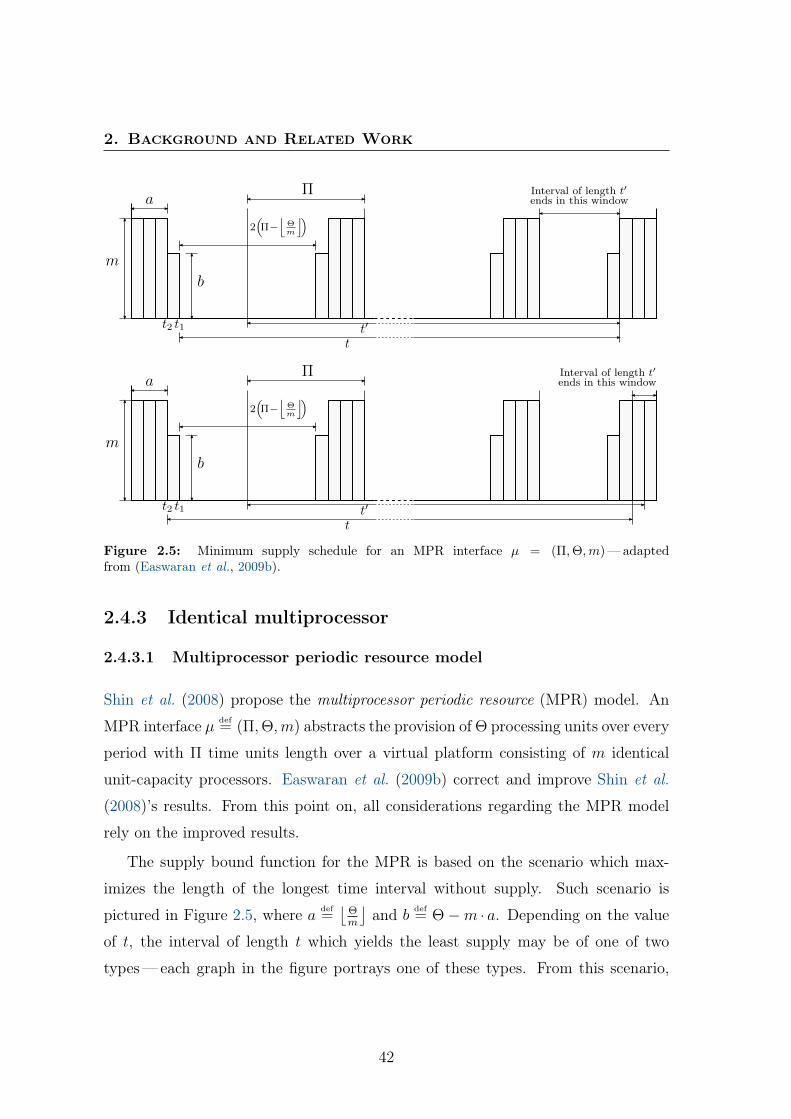
2. Background and Related Work

m

b

aΠ

2(Π−

⌊Θm

⌋)Interval of length t′ends in this window

t′

t

t2 t1

t2

m

b

a

t1

Π

2(Π−

⌊Θm

⌋)Interval of length t′ends in this window

t′

t

Figure 2.5: Minimum supply schedule for an MPR interface µ = (Π,Θ,m)—adaptedfrom (Easwaran et al., 2009b).

2.4.3 Identical multiprocessor

2.4.3.1 Multiprocessor periodic resource model

Shin et al. (2008) propose the multiprocessor periodic resource (MPR) model. An

MPR interface µ def= (Π,Θ,m) abstracts the provision of Θ processing units over every

period with Π time units length over a virtual platform consisting of m identical

unit-capacity processors. Easwaran et al. (2009b) correct and improve Shin et al.

(2008)’s results. From this point on, all considerations regarding the MPR model

rely on the improved results.

The supply bound function for the MPR is based on the scenario which max-

imizes the length of the longest time interval without supply. Such scenario is

pictured in Figure 2.5, where a def=⌊

Θm

⌋and b def

= Θ−m · a. Depending on the value

of t, the interval of length t which yields the least supply may be of one of two

types—each graph in the figure portrays one of these types. From this scenario,

42

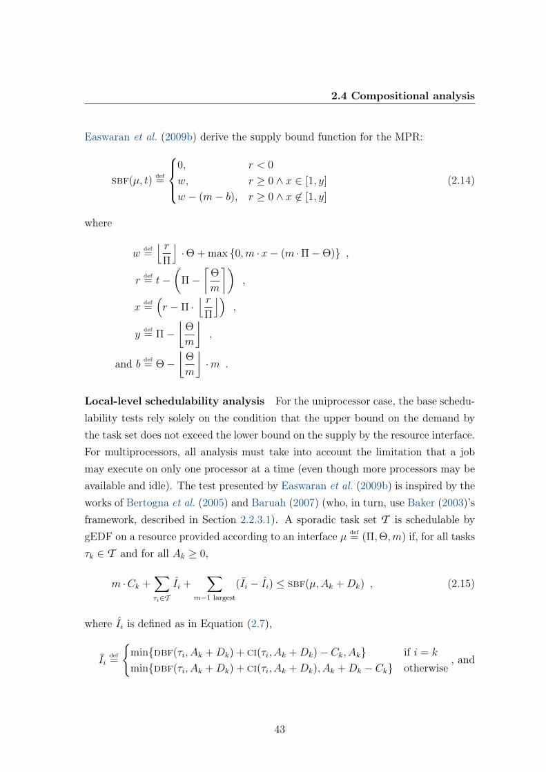
2.4 Compositional analysis

Easwaran et al. (2009b) derive the supply bound function for the MPR:

sbf(µ, t)def=

0, r < 0

w, r ≥ 0 ∧ x ∈ [1, y]

w − (m− b), r ≥ 0 ∧ x 6∈ [1, y]

(2.14)

where

wdef=⌊ r

Π

⌋· Θ + max {0,m ·x− (m · Π−Θ)} ,

rdef= t−

(Π−

⌈Θ

m

⌉),

xdef=(r − Π ·

⌊ rΠ

⌋),

ydef= Π−

⌊Θ

m

⌋,

and b def= Θ−

⌊Θ

m

⌋·m .

Local-level schedulability analysis For the uniprocessor case, the base schedu-lability tests rely solely on the condition that the upper bound on the demand bythe task set does not exceed the lower bound on the supply by the resource interface.For multiprocessors, all analysis must take into account the limitation that a jobmay execute on only one processor at a time (even though more processors may beavailable and idle). The test presented by Easwaran et al. (2009b) is inspired by theworks of Bertogna et al. (2005) and Baruah (2007) (who, in turn, use Baker (2003)’sframework, described in Section 2.2.3.1). A sporadic task set T is schedulable bygEDF on a resource provided according to an interface µ def

= (Π,Θ,m) if, for all tasksτk ∈ T and for all Ak ≥ 0,

m ·Ck +∑τi∈T

Ii +∑

m−1 largest

(Ii − Ii) ≤ sbf(µ,Ak +Dk) , (2.15)

where Ii is defined as in Equation (2.7),

Iidef=

{min{dbf(τi, Ak +Dk) + ci(τi, Ak +Dk)− Ck, Ak} if i = k

min{dbf(τi, Ak +Dk) + ci(τi, Ak +Dk), Ak +Dk − Ck} otherwise, and

43

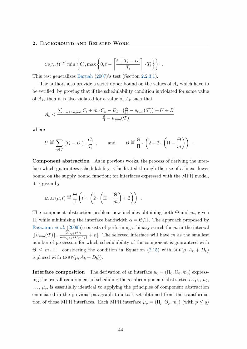
2. Background and Related Work

ci(τi, t)def= min

{Ci,max

{0, t−

⌈t+ Ti −Di

Ti

⌉·Ti}}

.

This test generalizes Baruah (2007)’s test (Section 2.2.3.1).The authors also provide a strict upper bound on the values of Ak which have to

be verified, by proving that if the schedulability condition is violated for some valueof Ak, then it is also violated for a value of Ak such that

Ak <

∑m−1 largestCi +m ·Ck −Dk ·

(ΘΠ− usum(T )

)+ U +B

ΘΠ− usum(T )

where

Udef=∑τi∈T

(Ti −Di) ·CiTi

, and Bdef=

Θ

Π·(

2 + 2 ·(

Π− Θ

m

)).

Component abstraction As in previous works, the process of deriving the inter-face which guarantees schedulability is facilitated through the use of a linear lowerbound on the supply bound function; for interfaces expressed with the MPR model,it is given by

lsbf(µ, t)def=

Θ

Π

(t−(

2 ·(

Π− Θ

m

)+ 2

)).

The component abstraction problem now includes obtaining both Θ and m, givenΠ, while minimizing the interface bandwidth α = Θ/Π. The approach proposed byEaswaran et al. (2009b) consists of performing a binary search for m in the interval[dusum(T )e ,

∑τi∈T Ci

minτi∈T {Di−Ci}+ n]. The selected interface will have m as the smallest

number of processors for which schedulability of the component is guaranteed withΘ ≤ m · Π—considering the condition in Equation (2.15) with sbf(µ,Ak + Dk)

replaced with lsbf(µ,Ak +Dk)).

Interface composition The derivation of an interface µ0 = (Π0,Θ0,m0) express-ing the overall requirement of scheduling the q subcomponents abstracted as µ1, µ2,. . . , µq, is essentially identical to applying the principles of component abstractionenunciated in the previous paragraph to a task set obtained from the transforma-tion of those MPR interfaces. Each MPR interface µp = (Πp,Θp,mp) (with p ≤ q)

44

2.4 Compositional analysis

is transformed into a task set T (µp) def={τ

(µp)i

}mi=1

with total utilization Θp. With

b = Θp −mp ·⌊

Θpmp

⌋and k = bbc, each interface task τ (µp)

idef=(T

(µp)i , C

(µp)i , D

(µp)i

)is

derived as follows:

• if i ≤ ki, τ(µp)i =

(Πp,⌊

Θpmp

⌋+ 1,Πp

);

• if i = ki + 1, τ (µp)i =

(Πp,⌊

Θpmp

⌋+ b− k ·

⌊bk

⌋,Πp

);

• otherwise, τ (µp)i =

(Πp,⌊

Θpmp

⌋,Πp

).

The interface µ0 is derived so as to guarantee that the task set⋃qp=1 T (µp) is

schedulable; more specifically, m0 will be the minimum number of processors found

to allow deriving a feasible interface. By definition, m0 lies within the interval[minqp=1 mp,

∑qp=1mp

].

2.4.3.2 Multi Supply Function

Bini et al. (2009b) point out that the advantage of the simplicity of the MPR ap-

proach, of having a common period and an aggregate contribution for all processors,

has a pessimistic component abstraction as a drawback. The authors then propose

the Multi Supply Function abstraction, which consists of a set of m supply bound

functions {sbf(Rk, t)}mk=1, where each function corresponds to the minimum amount

of availability of each virtual processor—abstracted with an interface Rk which can

be expressed using uniprocessor resource models (thus employing the respective

supply bound functions). Based on this possibility, they propose the Multi-(α,∆)

abstraction, in which each virtual processor is expressed using (Mok et al., 2001)’s

bounded-delay resource model. It renders a special case of a Multi Supply Function

which takes advantage of the simple definition of the supply bound function for the

bounded-delay resource model (see Equation (2.12)).

However different the virtual processors may be, the work of Bini et al. (2009b)

assumes that all of them correspond to partial availability of identical unit-capacity

physical processors.

45

2. Background and Related Work

Local-level schedulability analysis Bini et al. (2009b) provide sufficient schedu-lability tests for constrained-deadline sporadic task sets, with variations to accommo-date local-level scheduling (over a Multi Supply Function) according to (i) gEDF;(ii) any global fixed task priority algorithm; and (iii) any work-conserving algo-rithm.

Component abstraction / Interface composition Bini et al. (2009b) do notprovide component abstraction neither interface composition results for the MultiSupply Function abstraction. In a related work, Buttazzo et al. (2010, 2011) pro-pose a method for allocating a parallel real-time application, described as a set oftasks with time and precedence constraints, on a multicore platform. To achievemodularity and simplify portability of applications on different multicore platforms,the authors use the Multi Supply Function.

2.4.3.3 Parallel Supply Function

Bini et al. (2009a) propose the Parallel Supply Function to abstract resource pro-vision to a component. Their abstraction consists of m functions psfk(t), each oneexpressing the minimum amount of resource provided to the component, with par-allelism at most k, within every time interval of length t. This allows lifting theassumption (used in the MPR and Parallel Supply Function models) that periods(and hence resource provisions) are synchronized among all processors.

Local-level schedulability analysis For the Parallel Supply Function, Bini et al.(2009a) present two sufficient schedulability tests considering gEDF as the local-levelscheduler. The first employs the notion of forced-forward demand bound functionproposed by Baruah et al. (2009). The second is, like Easwaran et al. (2009b)’s testfor the MPR model, inspired by Bertogna et al. (2005).

Component abstraction / Interface composition Bini et al. (2009a) do notapproach the issue of component abstraction (and, consequently, interface compo-sition), which in this case corresponds to deriving the m level-j supply functionsto guarantee schedulability. Lipari & Bini (2010) demonstrate that component ab-straction with the Parallel Supply Function model is too complex.

46

2.4 Compositional analysis

2.4.3.4 Bounded-Delay Multipartition

(Lipari & Bini, 2010) propose the Bounded-Delay Multipartition, a new interface

model that allows the designer to balance resource usage versus flexibility in selecting

the virtual platform parameters. It borrows, on the one hand, from the bounded-

delay resource model and, on the other hand, from the Parallel Supply Function. A

Bounded-Delay Multipartition interface I def= (m,∆, {βk}mk=1), with

• ∆ ≥ 0;

• 0 ≤ βk − βk−1 ≤ 1, for all 1 ≤ k ≤ m; and

• βk − βk−1 ≤ βk+1 − βk, for all 1 ≤ k ≤ m;

if, for all resource allocations compatible with it, the Parallel Supply Functions are

psfk(t) ≥ βk · max(0, t−∆), for all 1 ≤ k ≤ m .

Each βk expresses the cumulative bandwidth provided with parallelism at most k,

whereas the ∆ parameter is the interface delay (for the bounded-delay multiparti-

tion, this is length of the longest interval with no guaranteed resource supply).

Compared to the MPR model, the authors lift the assumption that the periods

are synchronized across processors. Under this scenario, it is not possible to derive

a worst-case resource allocation for the MPR; for the Bounded-Delay Multipartition

the authors are able to prove that the worst-case resource allocation for a given

I = (m,∆, {βk}mk=1) is the set of m bounded-delay resource interfaces {(αk,∆)}mk=1,

with αk = βk − βk−1, for all 1 ≤ k ≤ m.

Local-level schedulability analysis Since the definition of a Bounded-Delay

Multipartition relies on properties attached to the Parallel Supply Function, schedu-

lability analysis can be performed with the tests proposed by Bini et al. (2009a) for

the latter. (Lipari & Bini, 2010) reformulate one of those tests, presenting schedula-

bility conditions for both gEDF and global fixed task priority local-level schedulers.

47

2. Background and Related Work

Component abstraction Lipari & Bini (2010) present a definition of the schedu-

lability region of a real-time application. The specific interface (namely, its ∆ pa-

rameter) can be chosen so as to constitute a compromise between schedulability and

overhead.

Interface composition To bind the virtual resource allocations on an identi-

cal multiprocessor physical platform. Lipari & Bini (2010) present an algorithm

called Fluid Best-Fit. The algorithm can be summarized as consisting of a Best

Fit partitioning (Section 2.2.2) of the worst-case allocation of each Bounded-Delay

Multipartition interface, followed by bandwidth modifications.

2.5 Technological support to TSP

In this section we survey the existing technical support to TSP systems, with respect

to both operating system support and tools to support the verification of temporal

properties in the integration phase of TSP system development. Due to its tighter

connection to industry practice, contains a significant amount of references to web-

sites, whose locations are provided in footnotes and have been verified to be correct

and available at the time of writing.7

2.5.1 Operating system support

The purpose of this subsection, where we survey the current state of practice, is

twofold. On the one hand, the existing solutions have varying degrees of support

to multicore and are, as such, candidates to improvement as per the architectural

considerations done in Section 3.2. On the other hand, even without such improve-

ments, systems based on the surveyed solutions can be represented using the system

model we propose in Section 3.3, and are potential targets for the application of the

principles and tools presented in this dissertation (Chapters 4 and 5, respectively).

7Last verification on July 31, 2013.

48

2.5 Technological support to TSP

2.5.1.1 PikeOS

PikeOS8 is a commercial microkernel-based real-time operating system (RTOS),developed by SYSGO. While initially implementing the L4 version 2.0 kernel appli-cation programming interface, the developers of PikeOS have identified issues withL4 version 2.0 and, while maintaining the base principles, have deeply modified theprogramming interface. Kaiser & Wagner (2007a) expose how PikeOS evolved, de-scribing the aforementioned issues and how they were approached. In this survey,we will only focus on the characteristics which differentiate PikeOS from other TSPoperating systems in terms of scheduling.

The PikeOS microkernel provides a more complex partition scheduling mecha-nism than the one defined in ARINC 653 (AEEC, 1997). At each instant, besides oneof the application time partitions (with a task set Ti), an additional time partitionis always active (the background partition, running a task set T0). The schedulerwill always select to be executed the highest priority task in Ti ∪T0. In the scope ofthis scheduling scheme, task priority definition plays a major role in offering flexi-bility to handle the coexistence of time-triggered and event-triggered tasks (Kaiser& Wagner, 2007b).

SYSGO introduced, in PikeOS 3.1, the first DO-178B-compliant implementationof multicore support (McConnel, 2010). The current version, PikeOS 3.3, includesimprovements and increased support to multicore, resulting of SYSGO’s participa-tion in the European project RECOMP (RECOMP, 2011b; SYSGO, 2013).

2.5.1.2 DEOS

DEOS9 is a commercial RTOS for safety-critical applications in the military andaerospace domains. Originating in technology developed by Honeywell (under theacronym DEOS—Digital Engine Operating System), it is (since 2008) provided byDDC-I Inc. (as DEOS—DDC-I Embedded Operating System).

DEOS provides space partitioning at the process level, and time partitioning atthe thread level. In this regard, it departs greatly from the notion of TSP associated

8http://www.sysgo.com/products/pikeos-rtos-and-virtualization-concept/9http://www.ddci.com/products_deos.php

49

2. Background and Related Work

with other solutions and approaches, including the IMA and ARINC 653 specifica-tions (Binns, 2001a). Time partitioning is enforced by scheduling processes andthreads according to a Rate Monotonic policy, enhanced with a patented (Binns,2001b) slack scheduling extension. DEOS supports creating and deleting threadsin runtime, with budget respectively being received from and returned to the mainthread. Consequently, offline verification is intractable (requiring the simulation ofall the expectable combinations of processes, threads, and budgets), and calcula-tions such as schedulability analysis have to be done in execution time (Penix et al.,2000).

We could not assess the exact extent and characteristics of DEOS’s support tomulticore processors, especially regarding scheduling. DDC-I (2012)’s DEOS factsheet makes no mention thereto, and we could only find superficial mentions to DDC-I’s view on multicore support in web articles (Howard, 2011; King, 2011, 2013). Inan interview to Howard (2011), Tim King at DDC-I talks about the work beingdeveloped at the time with respect to adding multicore support to DEOS, namelythe approach of partitioning caches that are shared by processor cores. King (2011)defends that reclaiming unused slack improves the performance of multicore pro-cessors, but does not describe how DEOS’s slack scheduling operates over multipleprocessor cores. King (2013) reports experiments carried at DDC-I with respect tocache partitioning. Although tackling the multicore-related issue of cache partition-ing, the experiments are based on running Deos on only one processor core, whichno description of how Deos supports multicore.

2.5.1.3 XtratuM

Developed at the Polytechnical University of Valencia under a contract from CNES,XtratuM10 first started as a nanokernel satisfying the requisites of a hard real-time system (Masmano et al., 2005). XtratuM was since redesigned, and is now ahypervisor aiming to fulfill safety-critical real-time requirements. It features TSPcapabilities, supported on the fixed cyclic scheduling of partitions (time partitioning)and on having partitions run in user mode without sharing any memory (spacepartitioning). Masmano et al. (2009) describe the core functionality of XtratuM

10http://www.xtratum.org/

50

2.5 Technological support to TSP

and evaluate the overhead introduced by mechanisms such as context switch whencommuting between partitions, resorting to a prototype implementation on a SPARCLEON2 processor platform without a memory management unit (MMU); the lackof an MMU did not allow the implementation of space partitioning capabilities infull.

Masmano et al. (2010) port XtratuM to a SPARC LEON3 processor platformwith an MMU, thus allowing to implement full space partitioning. Albeit usingARINC 653 concepts and models, XtratuM does not follow the ARINC 653 (AEEC,1997) interface.

Contemporarily to the work presented in this dissertation, the XtratuM architec-ture was included and extended in the MultiPARTES (Multi-cores Partitioning forTrusted Embedded Systems) project.11 The MultiPARTES approach to multicore issimilar to the one adopted in this dissertation (Craveiro et al., 2011), taking advan-tage of multiprocessor for parallelism at both the local (intrapartition) and global(interpartition) level (Coronel & Crespo, 2012). In the scope of MultiPARTES, de laPuente et al. (2012) draw some considerations on scheduling partitioned systems onmulticore platforms. The authors acknowledge the work of Shin et al. (2008) oncompositional analysis on identical multiprocessors, but fail to acknowledge morerecent works (Bini et al., 2009a,b; Lipari & Bini, 2010). Non-identical multipro-cessors (both uniform and heterogeneous) are mentioned, but not specifically dealtwith.

2.5.1.4 VxWorks 653

VxWorks 653 Platform12 is Wind River’s commercial solution for ARINC 653/IMAsystems (Wind River, 2010). It includes the VxWorks 653 operating system, whichimplements the complete Application Executive (APEX) interface specified in AR-INC 653 (AEEC, 1997), including the optional service for multiple module schedulesdefined in Part 2 (AEEC, 2007). Time and space partitioning is supported by a two-level scheme to schedule MMU-protected partitions. Each partition runs an instanceof the vThreads partition operating system. Applications can be developed to runon vThreads using the ARINC 653 APEX interface, POSIX, C, C++, Ada, or Java.

11http://www.multipartes.eu/.12http://www.windriver.com/products/platforms/safety_critical_arinc_653/

51

2. Background and Related Work

In addition to the cyclic partition scheduling from ARINC 653, VxWorks 653

provides the ARINC Plus Priority-Preempting Scheduling (APPS) hybrid mode.

In APPS, the system can change to priority-preemptive scheduling. Examples of

situations when this might occur include the detection of idle time in a time slice

attributed to a partition, or an idle partition time slice. Under priority-preemptive

scheduling, the non-idle partition with the highest priority is scheduled to run during

the detected idle time of the current time slice.

Wind River (2010)’s product note for the VxWorks 653 Platform makes no men-

tion to multicore support. The only mention we could find is a statement by Joe

Wlad from Wind River, in an interview to Howard (2011), that “VxWorks 653 ...

supports multicore architectures”.

2.5.2 Scheduling analysis and simulation tools

In this section, we restrict our attention to tools which provide some degree of

support to hierarchical scheduling or TSP systems. With the exception of Grasp

(which we describe first), these tools are presented here as solutions upon which this

dissertation (namely Chapter 5) constitutes an improvement.

2.5.2.1 Grasp

Grasp13 is a trace visualization tool set. It supports the visualization of multiproces-

sor hierarchical scheduling traces. Traces are recorded from the target system (by

the Grasp Recorder or any other appropriate means) into Grasp’s own script-like

format, and displayed graphically by the Grasp Player (Holenderski et al., 2013).

The Grasp tool set does not support simulation and supports only a two-level

hierarchy. However, the Grasp Player reads traces in a simple text-based format

which can be recorded by other tools. In Chapter 5, we take advantage of this

feature, and use Grasp to visualize simulation results.

13http://www.win.tue.nl/san/grasp/

52

2.5 Technological support to TSP

2.5.2.2 Cheddar

Cheddar14 provides a set of scheduling algorithms and policies on which it is capableof performing feasibility tests and/or scheduling simulations for either uniprocessoror multiprocessor environments (Singhoff et al., 2004). In its latest versions, Ched-dar already supports schedulability analysis of ARINC 653-like time- and space-partitioned (TSP) systems to some extent (Singhoff et al., 2009). However, Ched-dar presents some limitations in its current support thereto. A partition schedulingtable (PST) is defined as an array of durations; besides presenting less usability,the current implementation limits the PST to having only one time window perpartition per major time frame (Craveiro et al., 2011).

2.5.2.3 CARTS

CARTS15 is an open-source compositional analysis tool for real-time systems, whichautomatically generates the components’ resource interfaces; it does not performsimulation (Phan et al., 2011). CARTS relies strongly upon some of the authors’ the-oretical results, namely Shin & Lee (2003)’s periodic resource model, Easwaran et al.(2007)’s explicit-deadline periodic resource model, and Easwaran et al. (2009a)’s AR-INC 653-specific approach (reviewed in Section 2.4.2.3). Although implemented inJava, CARTS does not take advantage of the latter’s object-oriented characteristics(inheritance, polymorphism, encapsulation—especially regarding the separation be-tween domain and user interface). This makes it difficult to be extended and, assuch, we chose to develop our proof-of-concept tool (Chapter 5) from scratch insteadof modifying CARTS.

2.5.2.4 Schesim

The open-source Schesim scheduling simulator16 supports two-level hierarchicalscheduling on uniprocessor. Regarding task scheduling, Schesim supports fixed taskpriority and EDF algorithm, both in uniprocessor and partitioned multiprocessorsettings (global multiprocessor scheduling is not supported).

14http://beru.univ-brest.fr/~singhoff/cheddar/15http://rtg.cis.upenn.edu/carts/16https://code.google.com/p/schesim/

53

2. Background and Related Work

Extending Schesim is not an easy task. In particular, adding a new schedulingalgorithm requires obtaining, understanding and modifying Schesim’s source code(Matsubara et al., 2012). Other than Matsubara et al. (2012)’s paper, all documen-tation (including comments in the source code) is in Japanese language only.

2.5.2.5 Xoncrete

Within the scope of the XtratuM hypervisor (Section 2.5.1.3), Brocal et al. (2010)describe the Xoncrete17 tool for scheduling analysis of ARINC 653-based TSP sys-tems. The scheduling analysis performed by Xoncrete relies on timing requirementinformation, not from tasks themselves, but rather sequences of tasks with temporalattributes called End-To-End Flows. The notions of End-To-End Flow, task andpartition are independent, in the sense that an End-To-End Flow can contain tasksfrom different partitions, and that one given task can appear as part of more thanone End-To-End Flow. The tool generates a schedule (partition plan) from theEnd-To-End Flow parameters, using EDF as the base scheduling policy.

2.5.2.6 SymTA/S

SymTA/S 18 is Symtavision’s model-based timing analysis and optimization com-mercial solution. Symtavision (2013)’s product note states support to ARINC 653,making no specific mention to any other hierarchical scheduling framework.

2.6 Summary

In this chapter, we have presented the fundamental background notions on real-timescheduling, followed by a survey of the state of art and of the state of practice. Inthe following chapters, we present the contributions of this dissertation, which arerelated as follows with the presented related works.

The TSP system architecture that we describe in Chapter 3, with improvementsto support multicore processors (Section 3.2), can serve as the basis for improvementsto the current operating system support to TSP Section 2.5.1). In Section 3.3, we

17http://www.fentiss.com/en/products/xoncrete.html18https://symtavision.com/symtas.html

54

2.6 Summary

propose modeling our improved TSP system architecture as a compositional schedul-ing framework (Section 2.4). This system model can be used to model systems builtaround the existing TSP solutions (Section 2.5.1), as well as other systems based onresource reservation frameworks or hierarchical scheduling frameworks.

Consequently, the compositional analysis that we propose in Chapter 4 can beapplied those systems. Our proposal extends results from classical real-time schedul-ing analysis (Section 2.2) and fills a void in state-of-the-art compositional analysis(Section 2.4).

The tool we developed in the scope of this dissertation (Chapter 5) is a proof ofconcept for improvements over the state-of-the-art tools we surveyed in Section 2.5.2.

55

Chapter 3

Architecture and Model forMultiprocessor Time- andSpace-Partitioned Systems

In this chapter we present our first contribution: a system architecture definitionand formal model for multiprocessor time- and space-partitioned (TSP) systems. Westart (Section 3.1) by briefly presenting the reference architecture for uniprocessorTSP systems upon which we improve. Then, in Section 3.2, we discuss the gap tomultiprocessor in the state of the art, and present an improved system architecturewhich tackles such issues. In Section 3.3 we present a system model which allowsformal reasoning upon TSP systems which use multiprocessor platforms, with eitheridentical or non-identical processors; our system model is directed towards composi-tional analysis, and is applicable to many of the state of the art approaches regardingresource reservations and hierarchical scheduling.

3.1 Architecture overview

The architecture design, improved in the early stages of this dissertation’s work(Rufino et al., 2010), evolved from a proof of feasibility for adding ARINC 653 sup-port to the Real-Time Executive for Multiprocessor Systems (RTEMS) to a multi-OS (operating system) TSP architecture (Rufino et al., 2007). Its modular design

57

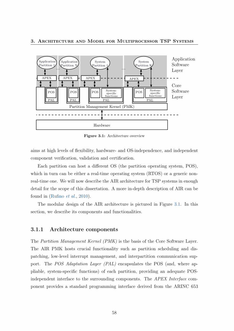
3. Architecture and Model for Multiprocessor TSP Systems

Partition Management Kernel (PMK)

Hardware

APEX APEX APEX APEX

ApplicationSoftwareLayer

CoreSoftwareLayer

POS POS POS POS System-specificfunctions

System-specificfunctions

ApplicationPartition 1

ApplicationPartition N

SystemPartition 1

SystemPartition K

PAL PAL PAL PAL

... ...

Figure 3.1: Architecture overview

aims at high levels of flexibility, hardware- and OS-independence, and independent

component verification, validation and certification.

Each partition can host a different OS (the partition operating system, POS),

which in turn can be either a real-time operating system (RTOS) or a generic non-

real-time one. We will now describe the AIR architecture for TSP systems in enough

detail for the scope of this dissertation. A more in-depth description of AIR can be

found in (Rufino et al., 2010).

The modular design of the AIR architecture is pictured in Figure 3.1. In this

section, we describe its components and functionalities.

3.1.1 Architecture components

The Partition Management Kernel (PMK) is the basis of the Core Software Layer.

The AIR PMK hosts crucial functionality such as partition scheduling and dis-

patching, low-level interrupt management, and interpartition communication sup-

port. The POS Adaptation Layer (PAL) encapsulates the POS (and, where ap-

pliable, system-specific functions) of each partition, providing an adequate POS-

independent interface to the surrounding components. The APEX Interface com-

ponent provides a standard programming interface derived from the ARINC 653

58

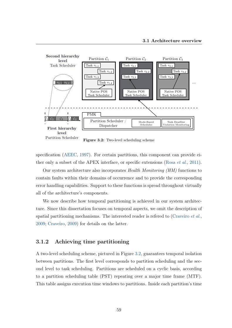
3.1 Architecture overview

τ2,1 τ2,2

Native POSTask Scheduler

PMK

Partition Scheduler /Dispatcher

Task DeadlineViolation Monitoring

Mode-BasedSchedules

Task τ1,1

Task τ1,2

Task τ1,3

Task τ1,4

Native POSTask Scheduler

Task τ2,1

Task τ2,2

Task τ2,3

Native POSTask Scheduler

Task τ3,1

Task τ3,2

Task τ3,3

Partition C1 Partition C2 Partition C3

...

Second hierarchylevel

Task Scheduler

First hierarchylevel

Partition Scheduler

C1 C2 C3 C1 C2

Figure 3.2: Two-level scheduling scheme

specification (AEEC, 1997). For certain partitions, this component can provide ei-

ther only a subset of the APEX interface, or specific extensions (Rosa et al., 2011).

Our system architecture also incorporates Health Monitoring (HM) functions to

contain faults within their domains of occurrence and to provide the corresponding

error handling capabilities. Support to these functions is spread throughout virtually

all of the architecture’s components.

We now describe how temporal partitioning is achieved in our system architec-

ture. Since this dissertation focuses on temporal aspects, we omit the description of

spatial partitioning mechanisms. The interested reader is refered to (Craveiro et al.,

2009; Craveiro, 2009) for details on the latter.

3.1.2 Achieving time partitioning

A two-level scheduling scheme, pictured in Figure 3.2, guarantees temporal isolation

between partitions. The first level corresponds to partition scheduling and the sec-

ond level to task scheduling. Partitions are scheduled on a cyclic basis, according

to a partition scheduling table (PST) repeating over a major time frame (MTF).

This table assigns execution time windows to partitions. Inside each partition’s time

59

3. Architecture and Model for Multiprocessor TSP Systems

windows, its processes compete according to the POS’s native process scheduler.1

Our scheduling scheme is enriched with temporal adaptation mechanisms, suchas mode-based schedules and task deadline violation monitoring. We now cover onlythe essentials of these mechanisms in this section, so as to provide context for thecontributions described in the following sections—evolution to multiprocessor andsystem model. We provide detailed description of the implementation and operationof our adaptation mechanisms in Chapter 6.

3.1.2.1 Mode-based schedules

Instead of one fixed PST, the system can be configured with multiple PSTs, whichmay differ in terms of the MTF duration, of which partitions are scheduled, and ofhow much processor time is assigned to them. The system can then switch betweenthese PSTs; this is performed through a service call issued by an authorized and/ordedicated partition. To avoid violating temporal requirements, a PST switch requestis only effectively granted at the end of the ongoing MTF.

3.1.2.2 Task deadline violation monitoring

During system execution, it may be the case that a task exceeds its deadline. Thiscan be caused by a malfunction, by transient overload (e. g., due to abnormallyhigh event signaling rates), or by the underestimation of its worst-case executionrequirement at system configuration and integration time. Temporal partitioningensures that this issue does not propagate to partitions other than the one to whichthe task belongs. Nevertheless, it may be necessary or beneficial to monitor and actupon such events. In the case of SRT applications, deadline misses does not directlyconstitute a fault, but should be monitored in light of the consequent QoS (or lackthereof). For HRT applications, deadline misses should be detected and mitigatedas soon as possible to prevent serious consequences.

Our system architecture includes a lightweight mechanism for task deadline vi-olation monitoring, which then communicates these events to the appropriate HMhandler, defined by the application developer and/or by the system integrator.

1Partitions are denoted as C, which stands for component, for coherence with the component-based approach used in this dissertation.

60

3.2 Evolution for multiprocessor

Partition Management Kernel

APEX APEX

ApplicationSoftwareLayer

CoreSoftwareLayer

POS POS System-specificfunctions

SystemPartition

1

CPU Core CPU CoreHardware

Partition Management Kernel

APEX APEX

POS POS System-specificfunctions

SystemPartition

2

Memory Memory

ApplicationPartition 1

ApplicationPartition 2

(a)

Multicore-aware Partition Management Kernel (PMK)

APEX APEX APEX APEX

ApplicationSoftwareLayer

CoreSoftwareLayer

POS POS POS POS System-specificfunctions

System-specificfunctions

ApplicationPartition 1

ApplicationPartition 2

SystemPartition

1

SystemPartition

2

CPU Core CPU CoreHardware

Memory

(b)

Figure 3.3: Example comparison between (a) a multiprocessor system implemented as inter-connected uniprocessor TSP nodes, and (b) a multicore (or shared-memory multiprocessor) TSPsystem implemented with our proposal of an evolved architecture

3.2 Evolution for multiprocessor

Approaches targeting multiple processors, such as that suggested in ARINC 653(AEEC, 1997), imply replicating the core software layer. In the case of our architec-ture, this implies replicating the PMK, as we see in Figure 3.3a. This configurationis inevitable when the memory adressing spaces are private to each processor and/or they are physically separated (Patterson & Hennessy, 2009). In some cases,this configuration may even be advantageous— for instance, when integration with

61

3. Architecture and Model for Multiprocessor TSP Systems

legacy systems is involved. However, the replicated instances are independently

integrated and configured, and the partitions associated with each one would be

bound to a strong affinity to a processor right from integration time. This limits the

extent to which we can take advantage of shared-memory multiprocessor platforms

in general, and multicore processors in particular. On the one hand, a partitioned

scheduling approach (Section 2.2.2) is forced upon the system. As we have seen in

Section 2.2.3.1, the partitioned and global scheduling approaches are incomparable

(in the sense that none of them is strictly better than the other one), and it is de-

sirable to have a flexible way to opt for one or the other depending on the specific

system being configured. On the other hand, this approach limits the extent to

which we can explore the adaptation mechanisms present in the AIR architecture,

such as using redundancy and mode-based schedules to overcome a hardware failure.

To add both the desired capacity and flexibility, we propose an architectural

evolution whereby the core software layer is enhanced to take advantage of an un-

derlying shared-memory multiprocessor or multicore processor platform, as we show

in Figure 3.3b. The association between partitions and cores is thus more volatile,

as it can be expressed in configuration parameters common to all the cores and

designed to change dynamically (e. g., through mode-based partition schedules).

Our advanced TSP system architecture may take advantage of a shared-memory

multiprocessor or multicore processor platform in several ways, either in alternative

or cumulatively, related with scheduling parallelism and fault tolerance. Regarding

parallelism, upon which we focus in this dissertation, we propose

1. having multiple partitions simultaneously scheduling/dispatching their respec-

tive processes on distinct processor cores (interpartition parallelism); and/or

2. allowing some partitions to be assigned more than one processor core during

their active time windows, so as to parallelly execute multiple processes (in-

trapartition parallelism).

Other advantages concern enhanced spatial partitioning, and self-adaptive behavior

to cope with processor core failures.

62

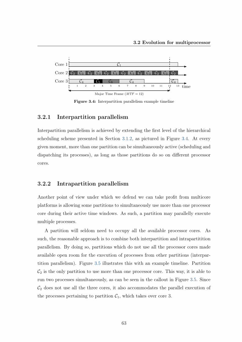
3.2 Evolution for multiprocessor

1 2 3 4 5 6 7 8 9 10 11 13120 time

C1

C4 C5 C6 C4

C3C2 C3C2 C3C2 C3C2 C3C2 C3C2 C2

C4

Core 1

Core 2

Core 3

Major Time Frame (MTF = 12)

Figure 3.4: Interpartition parallelism example timeline

3.2.1 Interpartition parallelism

Interpartition parallelism is achieved by extending the first level of the hierarchical

scheduling scheme presented in Section 3.1.2, as pictured in Figure 3.4. At every

given moment, more than one partition can be simultaneously active (scheduling and

dispatching its processes), as long as those partitions do so on different processor

cores.

3.2.2 Intrapartition parallelism

Another point of view under which we defend we can take profit from multicore

platforms is allowing some partitions to simultaneously use more than one processor

core during their active time windows. As such, a partition may parallelly execute

multiple processes.

A partition will seldom need to occupy all the available processor cores. As

such, the reasonable approach is to combine both interpartition and intrapartitition

parallelism. By doing so, partitions which do not use all the processor cores made

available open room for the execution of processes from other partitions (interpar-

tition parallelism). Figure 3.5 illustrates this with an example timeline. Partition

C2 is the only partition to use more than one processor core. This way, it is able to

run two processes simultaneously, as can be seen in the callout in Figure 3.5. Since

C2 does not use all the three cores, it also accommodates the parallel execution of

the processes pertaining to partition C1, which takes over core 3.

63

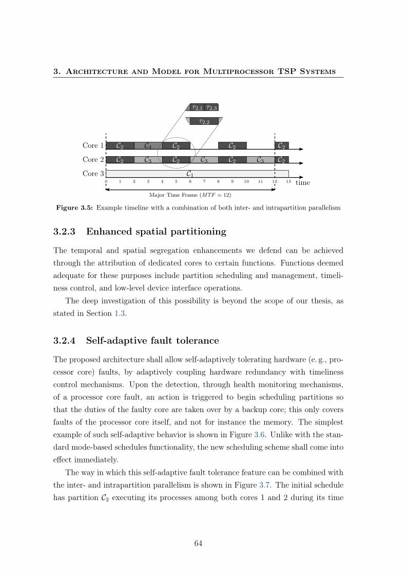
3. Architecture and Model for Multiprocessor TSP Systems

1 2 3 4 5 6 7 8 9 10 11 13120 timeC1

C3 C3 C3 C2

Core 1

Core 2

Core 3

C2 C2 C2 C2C4

C2 C2 C2

τ2,1

τ2,2

τ2,3

Major Time Frame (MTF = 12)

Figure 3.5: Example timeline with a combination of both inter- and intrapartition parallelism

3.2.3 Enhanced spatial partitioning

The temporal and spatial segregation enhancements we defend can be achievedthrough the attribution of dedicated cores to certain functions. Functions deemedadequate for these purposes include partition scheduling and management, timeli-ness control, and low-level device interface operations.

The deep investigation of this possibility is beyond the scope of our thesis, asstated in Section 1.3.

3.2.4 Self-adaptive fault tolerance

The proposed architecture shall allow self-adaptively tolerating hardware (e. g., pro-cessor core) faults, by adaptively coupling hardware redundancy with timelinesscontrol mechanisms. Upon the detection, through health monitoring mechanisms,of a processor core fault, an action is triggered to begin scheduling partitions sothat the duties of the faulty core are taken over by a backup core; this only coversfaults of the processor core itself, and not for instance the memory. The simplestexample of such self-adaptive behavior is shown in Figure 3.6. Unlike with the stan-dard mode-based schedules functionality, the new scheduling scheme shall come intoeffect immediately.

The way in which this self-adaptive fault tolerance feature can be combined withthe inter- and intrapartition parallelism is shown in Figure 3.7. The initial schedulehas partition C2 executing its processes among both cores 1 and 2 during its time

64

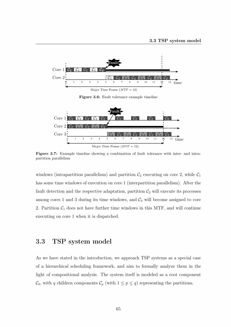
3.3 TSP system model

1 2 3 4 5 6 7 8 9 10 11 13120 time

C1C2 C2

C3C2 C3C2 C3C2

Core 1

Core 2

Major Time Frame (MTF = 12)

C2 C2 C1

Fault!

C2

C2

C1

Figure 3.6: Fault tolerance example timeline

1 2 3 4 5 6 7 8 9 10 11 13120 time

C1

C3C2 C3C2

C3

C2

C3C2 C3C2 C3C2

C2

Core 1

Core 2

Core 3

Major Time Frame (MTF = 12)

C2 C2 C1 C2 C2 C2 C2

Fault!

C2

C2

Figure 3.7: Example timeline showing a combination of fault tolerance with inter- and intra-partition parallelism

windows (intrapartition parallelism) and partition C3 executing on core 2, while C1

has some time windows of execution on core 1 (interpartition parallelism). After the

fault detection and the respective adaptation, partition C2 will execute its processes

among cores 1 and 3 during its time windows, and C3 will become assigned to core

2. Partition C1 does not have further time windows in this MTF, and will continue

executing on core 1 when it is dispatched.

3.3 TSP system model

As we have stated in the introduction, we approach TSP systems as a special case

of a hierarchical scheduling framework, and aim to formally analyze them in the

light of compositional analysis. The system itself is modeled as a root component

C0, with q children components Cp (with 1 ≤ p ≤ q) representing the partitions.

65

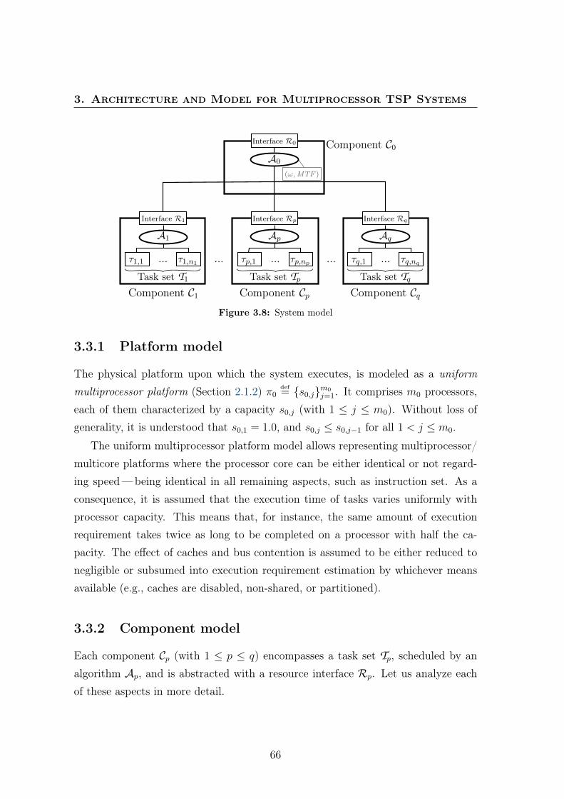
3. Architecture and Model for Multiprocessor TSP Systems

A0

A1 Aq

τ1,1

Component C0

Component C1 Component Cq

Interface R1

Ap

Component Cp

(ω,MTF )

...τ1,n1...Task set T1

τp,1 ...τp,np...Task set Tp

τq,1 τq,nq...Task set Tq

Interface Rp Interface Rq

Interface R0

Figure 3.8: System model

3.3.1 Platform model

The physical platform upon which the system executes, is modeled as a uniformmultiprocessor platform (Section 2.1.2) π0

def= {s0,j}m0

j=1. It comprises m0 processors,each of them characterized by a capacity s0,j (with 1 ≤ j ≤ m0). Without loss ofgenerality, it is understood that s0,1 = 1.0, and s0,j ≤ s0,j−1 for all 1 < j ≤ m0.

The uniform multiprocessor platform model allows representing multiprocessor/multicore platforms where the processor core can be either identical or not regard-ing speed—being identical in all remaining aspects, such as instruction set. As aconsequence, it is assumed that the execution time of tasks varies uniformly withprocessor capacity. This means that, for instance, the same amount of executionrequirement takes twice as long to be completed on a processor with half the ca-pacity. The effect of caches and bus contention is assumed to be either reduced tonegligible or subsumed into execution requirement estimation by whichever meansavailable (e.g., caches are disabled, non-shared, or partitioned).

3.3.2 Component model

Each component Cp (with 1 ≤ p ≤ q) encompasses a task set Tp, scheduled by analgorithm Ap, and is abstracted with a resource interface Rp. Let us analyze eachof these aspects in more detail.

66

3.3 TSP system model

3.3.2.1 Task model

The task set of each component, Tp, is composed of np constrained-deadline sporadictasks (Section 2.1.1) τp,i

def= (Tp,i, Cp,i, Dp,i). As we have seen in Section 2.1.1.1, a

sporadic task represents an unbounded sequence of jobs, with execution requirementat most Cp,i, with two consecutive jobs being released at least Tp,i time units apart.The worst-case execution requirement is assumed to have been correctly derived,and corresponds to the worst-case execution time on the fastest processor considered(i.e., the processor with schedulable utilizaton of 1.0 units of execution per unit oftime).

3.3.2.2 Scheduling algorithm

Each component’s scheduling algorithm Ap (for p > 1) is independent from theremaining components, and may come in the form of any scheduling algorithmcapable of scheduling constrained-deadline sporadic tasks on the platform providedby the resource interface Rp.

In this dissertation, we will focus on gEDF—global fixed job priority schedulingon a multiprocessor platform.

3.3.2.3 Resource model

The resource interface of each component, Rp, has a dual role of abstraction:

1. to component Cp, its resource interface Rp hides the details of how it receivesresource into a virtual processing platform; it is upon this restricted view ofthe processing platform that scheduling algorithm Ap makes its decisions;

2. to the parent component C0, each resource interface Rp hides how the respec-tive component Cp is internally structured; it is upon this restricted view of thechildren components of C0 that scheduling algorithm A0 makes its decisions.

The model used to express the resource interface may vary. In Chapter 4, we proposea model to express resource interfaces on uniform multiprocessor platforms. Sincethe latter generalize other platform models, we are as well able to express resourceinterfaces on uniprocessor and identical multiprocessor platforms.

67

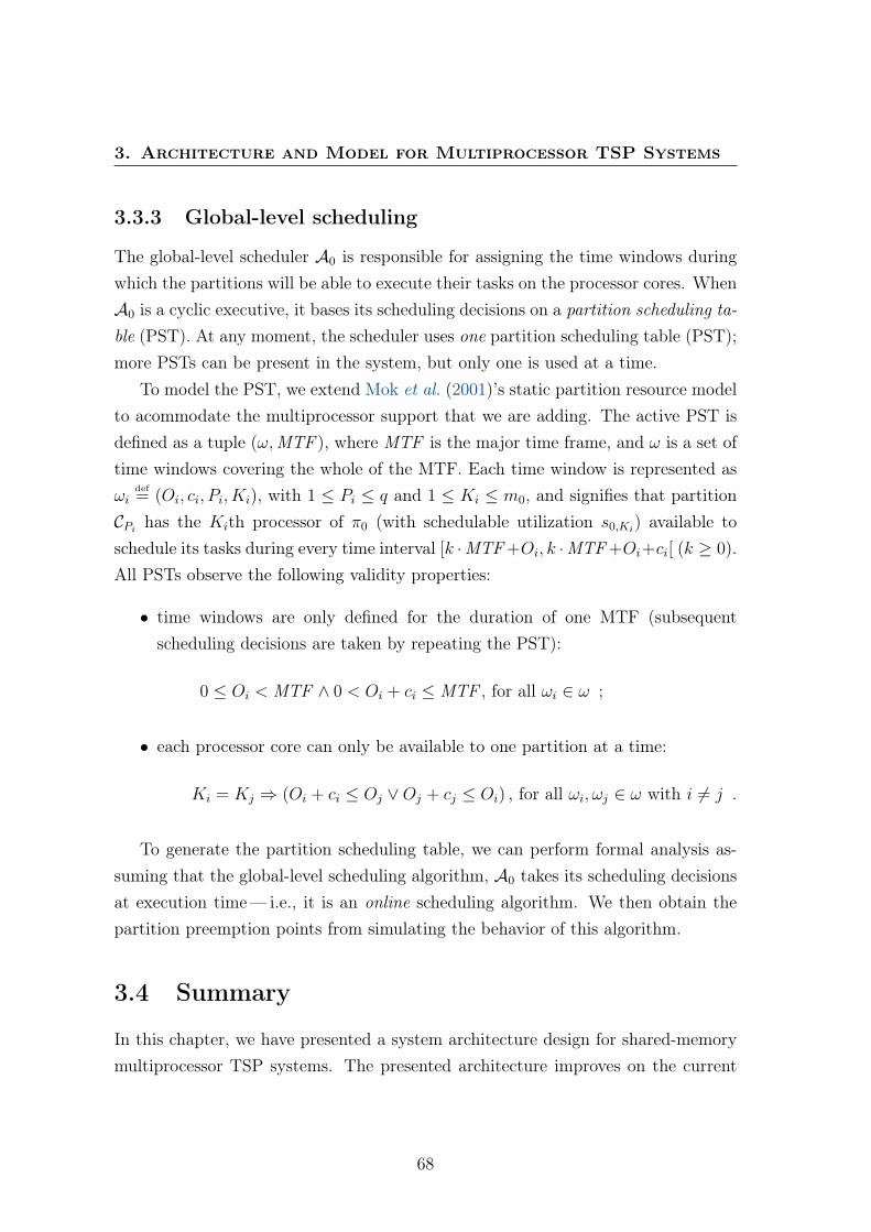
3. Architecture and Model for Multiprocessor TSP Systems

3.3.3 Global-level scheduling

The global-level scheduler A0 is responsible for assigning the time windows duringwhich the partitions will be able to execute their tasks on the processor cores. WhenA0 is a cyclic executive, it bases its scheduling decisions on a partition scheduling ta-ble (PST). At any moment, the scheduler uses one partition scheduling table (PST);more PSTs can be present in the system, but only one is used at a time.

To model the PST, we extend Mok et al. (2001)’s static partition resource modelto acommodate the multiprocessor support that we are adding. The active PST isdefined as a tuple (ω,MTF ), where MTF is the major time frame, and ω is a set oftime windows covering the whole of the MTF. Each time window is represented asωi

def= (Oi, ci, Pi, Ki), with 1 ≤ Pi ≤ q and 1 ≤ Ki ≤ m0, and signifies that partition

CPi has the Kith processor of π0 (with schedulable utilization s0,Ki) available toschedule its tasks during every time interval [k ·MTF+Oi, k ·MTF+Oi+ci[ (k ≥ 0).All PSTs observe the following validity properties:

• time windows are only defined for the duration of one MTF (subsequentscheduling decisions are taken by repeating the PST):

0 ≤ Oi < MTF ∧ 0 < Oi + ci ≤ MTF , for all ωi ∈ ω ;

• each processor core can only be available to one partition at a time:

Ki = Kj ⇒ (Oi + ci ≤ Oj ∨Oj + cj ≤ Oi) , for all ωi, ωj ∈ ω with i 6= j .

To generate the partition scheduling table, we can perform formal analysis as-suming that the global-level scheduling algorithm, A0 takes its scheduling decisionsat execution time— i.e., it is an online scheduling algorithm. We then obtain thepartition preemption points from simulating the behavior of this algorithm.

3.4 Summary

In this chapter, we have presented a system architecture design for shared-memorymultiprocessor TSP systems. The presented architecture improves on the current

68

3.4 Summary

state of art and practice by not demanding that the core software layer is repli-cated (with the consequent stronger affinity of partitions to processor cores). Thisimprovement, which is applicable to multicore processors, enables not only inter-partition parallelism, but also intrapartition parallelism (i.e., parallelism betweentasks in the same partitions) and adaptability/self-adaptability. Finally, we havepresented a system model for multiprocessor TSP systems, generalized as hierarchi-cal scheduling frameworks. This model allows us to perform formal reasoning onTSP systems, as we do in the next chapter. For the global-level scheduling, we willapproach formal reasoning under the assumption that A0 is an online algorithm. InChapter 5 we show how we obtain a partition scheduling table (to be used by a cyclicexecutive scheduler, as employed in safety-critical TSP systems) by simulating thebehavior the such an online algorithm.

69

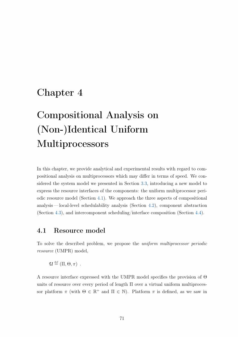
Chapter 4

Compositional Analysis on(Non-)Identical UniformMultiprocessors

In this chapter, we provide analytical and experimental results with regard to com-positional analysis on multiprocessors which may differ in terms of speed. We con-sidered the system model we presented in Section 3.3, introducing a new model toexpress the resource interfaces of the components: the uniform multiprocessor peri-odic resource model (Section 4.1). We approach the three aspects of compositionalanalysis— local-level schedulability analysis (Section 4.2), component abstraction(Section 4.3), and intercomponent scheduling/interface composition (Section 4.4).

4.1 Resource model

To solve the described problem, we propose the uniform multiprocessor periodicresource (UMPR) model,

U def= (Π,Θ, π) .

A resource interface expressed with the UMPR model specifies the provision of Θ

units of resource over every period of length Π over a virtual uniform multiproces-sor platform π (with Θ ∈ R+ and Π ∈ N). Platform π is defined, as we saw in

71

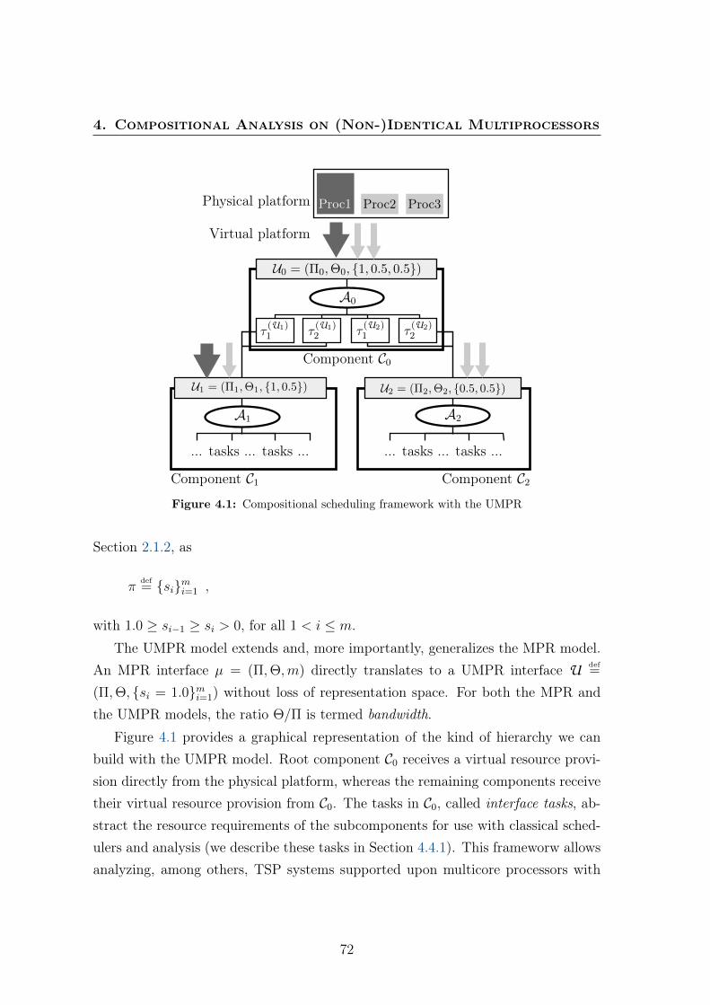
4. Compositional Analysis on (Non-)Identical Multiprocessors

A0

U0 = (Π0,Θ0, {1, 0.5, 0.5})

U1 = (Π1,Θ1, {1, 0.5}) U2 = (Π2,Θ2, {0.5, 0.5})

A1

Component C0

Component C1 Component C2

Virtual platform

Physical platform Proc1 Proc2 Proc3

A2

... tasks ... tasks ... ... tasks ... tasks ...

τ(U1)1 τ

(U1)2 τ

(U2)1 τ

(U2)2

Figure 4.1: Compositional scheduling framework with the UMPR

Section 2.1.2, as

πdef= {si}mi=1 ,

with 1.0 ≥ si−1 ≥ si > 0, for all 1 < i ≤ m.

The UMPR model extends and, more importantly, generalizes the MPR model.An MPR interface µ = (Π,Θ,m) directly translates to a UMPR interface U def

=

(Π,Θ, {si = 1.0}mi=1) without loss of representation space. For both the MPR andthe UMPR models, the ratio Θ/Π is termed bandwidth.

Figure 4.1 provides a graphical representation of the kind of hierarchy we canbuild with the UMPR model. Root component C0 receives a virtual resource provi-sion directly from the physical platform, whereas the remaining components receivetheir virtual resource provision from C0. The tasks in C0, called interface tasks, ab-stract the resource requirements of the subcomponents for use with classical sched-ulers and analysis (we describe these tasks in Section 4.4.1). This frameworw allowsanalyzing, among others, TSP systems supported upon multicore processors with

72

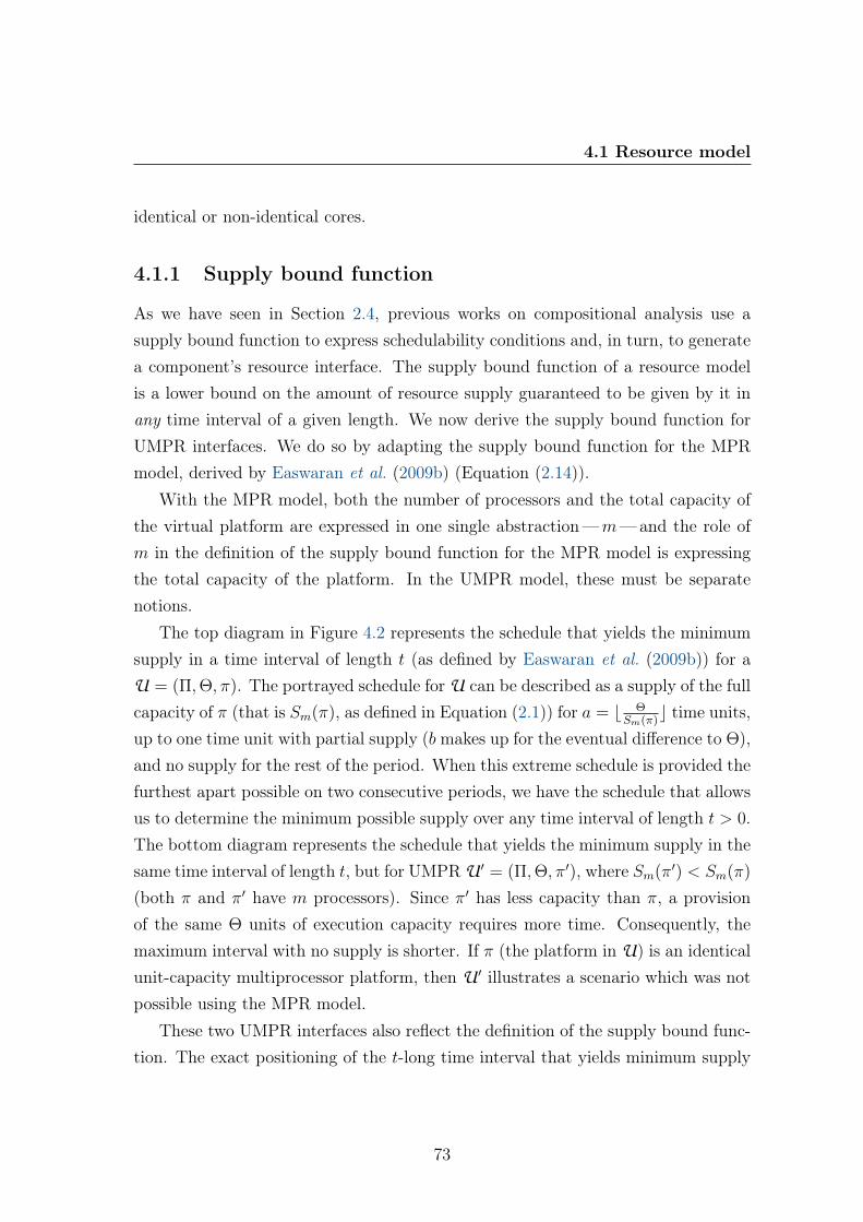
4.1 Resource model

identical or non-identical cores.

4.1.1 Supply bound function

As we have seen in Section 2.4, previous works on compositional analysis use asupply bound function to express schedulability conditions and, in turn, to generatea component’s resource interface. The supply bound function of a resource modelis a lower bound on the amount of resource supply guaranteed to be given by it inany time interval of a given length. We now derive the supply bound function forUMPR interfaces. We do so by adapting the supply bound function for the MPRmodel, derived by Easwaran et al. (2009b) (Equation (2.14)).

With the MPR model, both the number of processors and the total capacity ofthe virtual platform are expressed in one single abstraction—m—and the role ofm in the definition of the supply bound function for the MPR model is expressingthe total capacity of the platform. In the UMPR model, these must be separatenotions.

The top diagram in Figure 4.2 represents the schedule that yields the minimumsupply in a time interval of length t (as defined by Easwaran et al. (2009b)) for aU = (Π,Θ, π). The portrayed schedule for U can be described as a supply of the fullcapacity of π (that is Sm(π), as defined in Equation (2.1)) for a = b Θ

Sm(π)c time units,

up to one time unit with partial supply (b makes up for the eventual difference to Θ),and no supply for the rest of the period. When this extreme schedule is provided thefurthest apart possible on two consecutive periods, we have the schedule that allowsus to determine the minimum possible supply over any time interval of length t > 0.The bottom diagram represents the schedule that yields the minimum supply in thesame time interval of length t, but for UMPR U ′ = (Π,Θ, π′), where Sm(π′) < Sm(π)

(both π and π′ have m processors). Since π′ has less capacity than π, a provisionof the same Θ units of execution capacity requires more time. Consequently, themaximum interval with no supply is shorter. If π (the platform in U) is an identicalunit-capacity multiprocessor platform, then U ′ illustrates a scenario which was notpossible using the MPR model.

These two UMPR interfaces also reflect the definition of the supply bound func-tion. The exact positioning of the t-long time interval that yields minimum supply

73

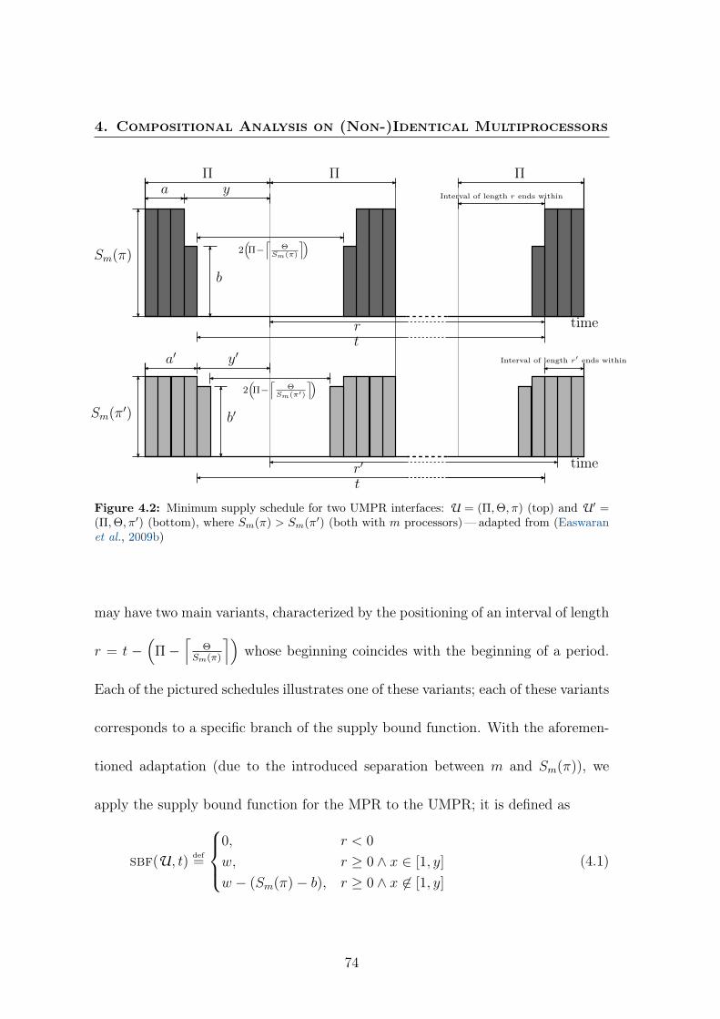
4. Compositional Analysis on (Non-)Identical Multiprocessors

Sm(π)

b

aΠΠ

2(Π−

⌈Θ

Sm(π)

⌉)

b′

2(Π−

⌈Θ

Sm(π′)

⌉)a′

Sm(π′)

time

Π

t

t

Interval of length r ends within

Interval of length r′ ends within

r

r′ time

y

y′

Figure 4.2: Minimum supply schedule for two UMPR interfaces: U = (Π,Θ, π) (top) and U′ =(Π,Θ, π′) (bottom), where Sm(π) > Sm(π′) (both with m processors)—adapted from (Easwaranet al., 2009b)

may have two main variants, characterized by the positioning of an interval of length

r = t −(

Π−⌈

ΘSm(π)

⌉)whose beginning coincides with the beginning of a period.

Each of the pictured schedules illustrates one of these variants; each of these variants

corresponds to a specific branch of the supply bound function. With the aforemen-

tioned adaptation (due to the introduced separation between m and Sm(π)), we

apply the supply bound function for the MPR to the UMPR; it is defined as

sbf(U, t)def=

0, r < 0

w, r ≥ 0 ∧ x ∈ [1, y]

w − (Sm(π)− b), r ≥ 0 ∧ x 6∈ [1, y]

(4.1)

74

4.1 Resource model

where

wdef=⌊ r

Π

⌋· Θ + max {0, Sm(π) ·x− (Sm(π) · Π−Θ)} ,

rdef=t−

(Π−

⌈Θ

Sm(π)

⌉),

xdef=(r − Π ·

⌊ rΠ

⌋),

ydef=Π−

⌊Θ

Sm(π)

⌋,

and b def=Θ−

⌊Θ

Sm(π)

⌋·Sm(π) .

When π is an identical multiprocessor platform, m = Sm(π), and the supply bound

function becomes identical to that of the equivalent MPR interface.

4.1.2 Linear lower bound on the supply bound function

To reduce the complexity of computations based on the supply bound function, it is

usual to resort to a linear lower bound on the latter. We are also able to adapt for

the UMPR the definition of the linear lower bound on the supply bound function,

lsbf(U, t), that Easwaran et al. (2009b) defined for the MPR:

lsbf(U, t)def=

Θ

Π

(t−(

2 ·(

Π− Θ

Sm(π)

)+ 2

)).

An important property of the lsbf is that lsbf(U, t) ≤ sbf(U, t), for all t > 0

(Easwaran et al., 2009b).

Figure 4.3 shows the plots of sbf and lsbf for the same two UMPR interfaces.

In conformity with the aforementioned discussion, the range of lengths t for which

there is no minimum guaranteed supply is greater for U than for U ′. Furthermore,

we can also see that, after the range of lengths t for which there is no minimum

guaranteed supply, the growth of the supply bound function repeats with a period

of Π.

75

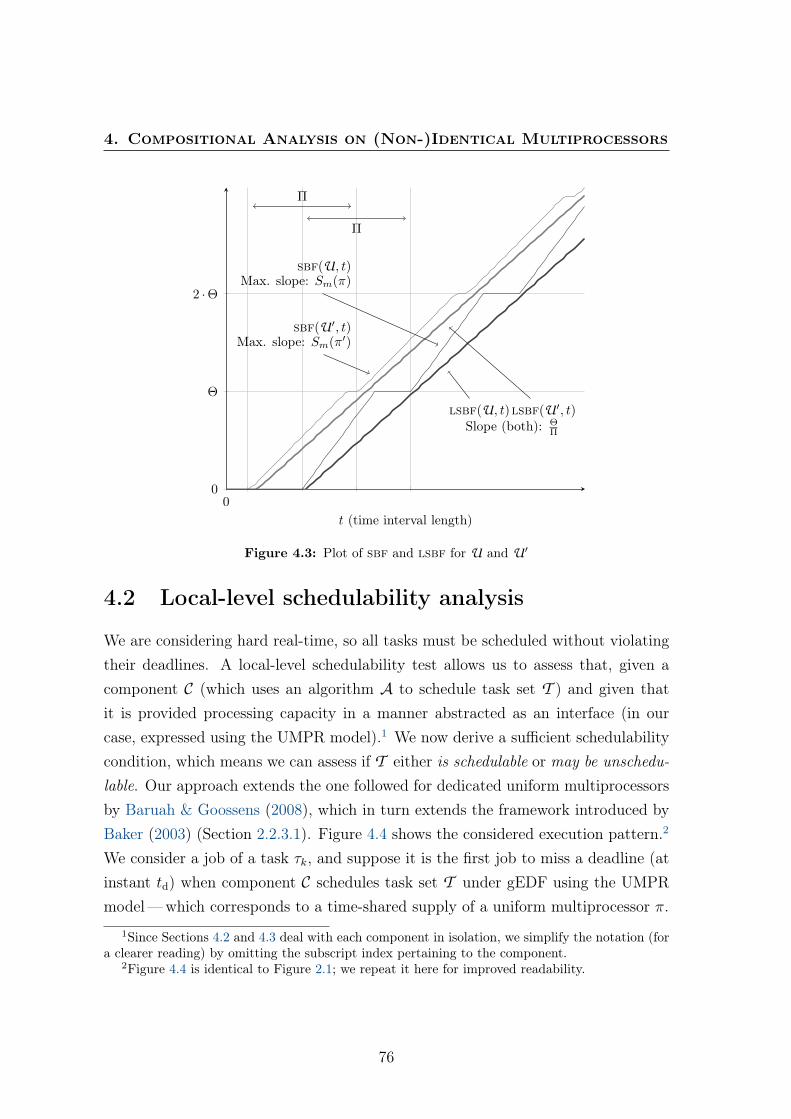
4. Compositional Analysis on (Non-)Identical Multiprocessors

00

Θ

2 · Θ

sbf(U′, t)Max. slope: Sm(π′)

sbf(U, t)Max. slope: Sm(π)

lsbf(U, t)lsbf(U′, t)Slope (both): Θ

Π

Π

Π

t (time interval length)

Figure 4.3: Plot of sbf and lsbf for U and U′

4.2 Local-level schedulability analysis

We are considering hard real-time, so all tasks must be scheduled without violatingtheir deadlines. A local-level schedulability test allows us to assess that, given acomponent C (which uses an algorithm A to schedule task set T ) and given thatit is provided processing capacity in a manner abstracted as an interface (in ourcase, expressed using the UMPR model).1 We now derive a sufficient schedulabilitycondition, which means we can assess if T either is schedulable or may be unschedu-lable. Our approach extends the one followed for dedicated uniform multiprocessorsby Baruah & Goossens (2008), which in turn extends the framework introduced byBaker (2003) (Section 2.2.3.1). Figure 4.4 shows the considered execution pattern.2

We consider a job of a task τk, and suppose it is the first job to miss a deadline (atinstant td) when component C schedules task set T under gEDF using the UMPRmodel—which corresponds to a time-shared supply of a uniform multiprocessor π.

1Since Sections 4.2 and 4.3 deal with each component in isolation, we simplify the notation (fora clearer reading) by omitting the subscript index pertaining to the component.

2Figure 4.4 is identical to Figure 2.1; we repeat it here for improved readability.

76

4.2 Local-level schedulability analysis

timeti t0 ta td

Di

φi Ak Dk

τi τk

deadline miss

Figure 4.4: Considered execution pattern.

We now follow the strategy used by Baruah & Goossens (2008), with the dueadaptation to the fact that we are dealing with a potentially non-dedicated resourcesupply. For this, we employ the function supply(C, t1, t2), which we have intro-duced in Section 2.4 and denotes the effective resource supply that component Creceives over the specific time interval [t1, t2[. This is different from the supplybound function, which denotes the minimum guaranteed resource supply the com-ponent receives over any time interval with a given length, according to its interface.Although we do not have a tractable way to compute this quantity, we acknowledgeits existence and will take advantage of its following properties:

• supply(C, t1, t2)+supply(C, t2, t3) = supply(C, t1, t3), for all values of t1, t2, t3such that t1 < t2 < t3;

• sbf(U, t2− t1) ≤ supply(C, t1, t2), for all values of t1, t2 such that t1 < t2; wewill call upon this property when deriving our schedulability condition.

4.2.1 Interference interval

The time interval we need to consider using this execution pattern is [t0, td[. Instanttd is the absolute deadline that τk misses. We perform our analysis over a scenarioin which only one job (of some task τk) misses a deadline at instant td; however,its reasoning and results still hold if this assumption is lifted.3 Baruah & Goossens(2008) do not point out this issue in their paper, but the same applies: although

3Example: consider that jobs of both τ1 and τ2 miss their deadlines, and both deadlines are attd. After breaking the tie, one of the jobs will have a priority lower than the other one; whetherthe lower-priority job is that of τ1 or τ2, it will not interfere with the higher-priority one. As such,only the higher-priority late job is relevant.

77

4. Compositional Analysis on (Non-)Identical Multiprocessors

they implicitly assume only one job misses its deadline at instant td, their analysis

is still valid otherwise.

We now determine which specific instant is t0. For this, let W (t) (with t ≤ td)

denote the cumulative job execution requirement for time interval [t, td[; this is

different from the demand bound function we saw in Section 2.2.1.2 (which is an

upper bound on one of the sources of this cumulative job execution requirement).

Let I`,c denote the total duration, over [ta, td[, for which exactly ` processors, the

slowest of which is sc, are busy scheduling jobs of component C (with 0 ≤ ` ≤ c < m),

and at least one processor in {sc+1, . . . , sm} is available (thus, idle). By definition

of gEDF:

1. since processor sc is busy, no processor in {s1, . . . , sc} can be available to the

component but idle; and

2. whenever there is an idle processor, τi’s job must be executing on one of the

processors in {s1, . . . , sc}.

Unlike when π is a dedicated platform (Baruah & Goossens, 2008), we cannot guar-

antee that, at each instant, τi is executing on one of the fastest processors in π, but

only that it is executing on one of the fastest processors available at that instant.

So, for each duration I`,c, the job is guaranteed to be executing on a processor of

speed, at least, sc. Therefore,

Ck >

m−1∑`=1

m∑c=`

sc · I`,c . (4.2)

The total amount of execution completed on C over the interval [ta, td[ is given

by the difference between the resource supply it receives— supply(C, ta, td)—and

the total capacity that was idled although available. For each duration I`,c, the

available capacity that is idled is upper bounded by the capacity of the m − c

slowest processors; as we have seen, no processor in {s1, . . . , sc} can be available but

idle. Since this amount is not sufficient for τk’s job to meet its deadline at td, we

78

4.2 Local-level schedulability analysis

have

W (ta) > supply(C, ta, td)−m−1∑`=1

m∑c=`

(Sm(π)− Sc(π)) · I`,c

= supply(C, ta, td)−m−1∑`=1

m∑c=`

Sm(π)− Sc(π)

sc· sc · I`,c

≥ supply(C, ta, td)− λ(π) ·m−1∑`=1

m∑c=`

sc · I`,c

(by definition of λ(π)—Equation (2.2))

> supply(C, ta, td)− λ(π) ·Ck

(by Equation (4.2))

= supply(C, ta, td)− λ(π) · δk ·Dk

≥ supply(C, ta, td)− λ(π) · δmax(T ) ·Dk .

Now let us consider a particular instant t0, which is formally defined as thesmallest value t ≤ ta such that W (t) ≥ supply(C, t, td) − λ(π) · δmax(T ) · (td − t).This means that t0 is the earliest instant t so that, in the time interval [t, ta[, noresource capacity available to C was idled. As a consequence, we can say that, foran arbitrarily small positive number ε, some processor was available to C but idle inthe time interval [t0 − ε, t0[.

4.2.2 Component demand

We have defined the interval we need to consider— that is [t0, td[. Next, we de-termine the cumulative execution that gEDF needs (but fails) to execute over thatinterval, denoted by W (t0). As we have seen, two sources contribute to W (t0):

• jobs with arrival times within [t0, td[ and deadline times within [t0, td]—thiscontribution includes the execution requirement of τk’s deadline-missing job,and is upper-bounded by

∑τi∈T dbf(τi, Ak +Dk) (where Ak = ta − t0); and

• jobs that arrive before instant t0 and carry in some execution to time interval[t0, td[—by construction of the execution pattern and by definition of the

79

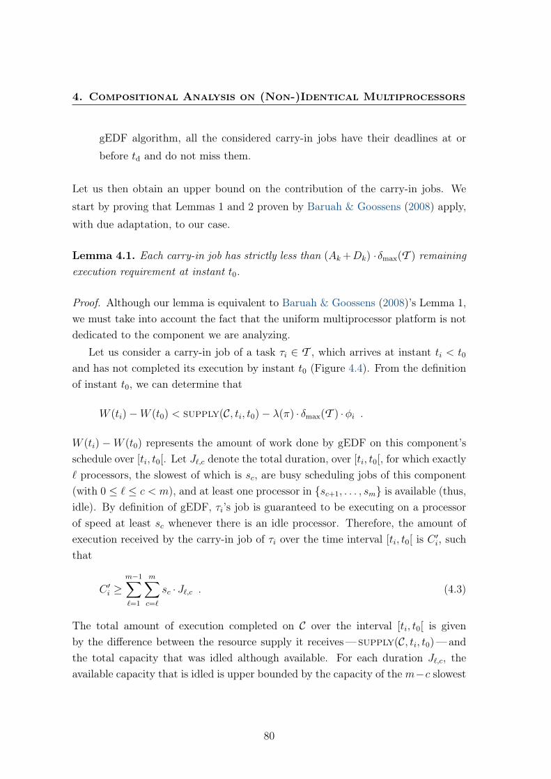
4. Compositional Analysis on (Non-)Identical Multiprocessors

gEDF algorithm, all the considered carry-in jobs have their deadlines at or

before td and do not miss them.

Let us then obtain an upper bound on the contribution of the carry-in jobs. We

start by proving that Lemmas 1 and 2 proven by Baruah & Goossens (2008) apply,

with due adaptation, to our case.

Lemma 4.1. Each carry-in job has strictly less than (Ak +Dk) · δmax(T ) remainingexecution requirement at instant t0.

Proof. Although our lemma is equivalent to Baruah & Goossens (2008)’s Lemma 1,we must take into account the fact that the uniform multiprocessor platform is notdedicated to the component we are analyzing.

Let us consider a carry-in job of a task τi ∈ T , which arrives at instant ti < t0

and has not completed its execution by instant t0 (Figure 4.4). From the definitionof instant t0, we can determine that

W (ti)−W (t0) < supply(C, ti, t0)− λ(π) · δmax(T ) ·φi .

W (ti) −W (t0) represents the amount of work done by gEDF on this component’sschedule over [ti, t0[. Let J`,c denote the total duration, over [ti, t0[, for which exactly` processors, the slowest of which is sc, are busy scheduling jobs of this component(with 0 ≤ ` ≤ c < m), and at least one processor in {sc+1, . . . , sm} is available (thus,idle). By definition of gEDF, τi’s job is guaranteed to be executing on a processorof speed at least sc whenever there is an idle processor. Therefore, the amount ofexecution received by the carry-in job of τi over the time interval [ti, t0[ is C ′i, suchthat

C ′i ≥m−1∑`=1

m∑c=`

sc · J`,c . (4.3)

The total amount of execution completed on C over the interval [ti, t0[ is givenby the difference between the resource supply it receives— supply(C, ti, t0)—andthe total capacity that was idled although available. For each duration J`,c, theavailable capacity that is idled is upper bounded by the capacity of the m−c slowest

80

4.2 Local-level schedulability analysis

processors. Since this amount is not sufficient for τk’s job to meet its deadline at td:

W (ti)−W (t0) > supply(C, ti, t0)−m−1∑`=1

m∑c=`

(Sm(π)− Sc(π)) · J`,c

So we have

−λ(π) · δmax(T ) ·φi >−m−1∑`=1

m∑c=`

(Sm(π)− Sc(π)) · J`,c

−λ(π) · δmax(T ) ·φi >−m−1∑`=1

m∑c=`

Sm(π)− Sc(π)

sc· sc · J`,c

−λ(π) · δmax(T ) ·φi >− λ(π) ·m−1∑`=1

m∑c=`

sc · J`,c

(by definition of λ(π)—Equation (2.2))

−λ(π) · δmax(T ) ·φi >− λ(π) ·C ′i

(by Equation (4.3))

C ′i > δmax(T ) ·φi

Since Ci = δi ·Di ≤ δmax(T ) ·Di, we have that

Ci − C ′i < δmax(T ) ·Di − δmax(T ) ·φi= δmax(T ) · (Di − φi) . (4.4)

By construction of the considered execution pattern, we have that the absolutedeadline of this τi’s job (ti +Di) is not greater than td, so

ti +Di − t0 ≤ td − t0Di − φi ≤ Ak +Dk

Replacing this in Equation (4.4) we prove the lemma. �

Lemma 4.2. There are, at most, ν = m− 1 carry-in jobs.

Proof. We use the same principle as Baruah & Goossens (2008), but are not able toreach an equally tight bound (cf. Equation (2.9)). Let ε denote an arbitrarily small

81

4. Compositional Analysis on (Non-)Identical Multiprocessors

positive number; by definition,W (t0−ε) < supply(C, t0−ε, td)−λ(π) · δmax(T ) · (Ak+

Dk + ε), whereas W (t0) ≥ supply(C, t0, td)− λ(π) · δmax(T ) · (Ak +Dk); hence:

W (t0 − ε)−W (t0) < supply(C, t0 − ε, t0)− λ(π) · δmax(T ) · ε,

which shows some processor was idled (although available to C) in [t0 − ε, t0[. Bydefinition of gEDF, this means all active jobs were executing; hence, the number ofcarry-in jobs is, at most, one less than the number of available processors. Sincewe do not possess a way to know exactly how many processors were available to Cin [t0 − ε, t0[, we are not able to tighten this bound further than the worst case (mprocessors available, m− 1 carry-in jobs). �

4.2.3 Sufficient local-level schedulability test

With the conditions proven in Lemmas 4.1 and 4.2 we are able to formulate a

necessary condition for unschedulability of C, from which we then derive the sufficient

schedulability condition.

Lemma 4.3. If a component C, comprising a virtual uniform multiprocessor plat-form π and a sporadic task set T , is not schedulable under gEDF using UMPR modelU = (Π,Θ, π), then for some τk ∈ T and some Ak ≥ 0∑τi∈T

dbf(τi, Ak+Dk)+(ν + λ(π)) · (Ak+Dk) · δmax(T ) > sbf(U, Ak+Dk) , (4.5)

Proof. We are now able to establish a strict upper bound on W (t0), based on thetwo sources that contribute to such execution requirement. Jobs that have ar-rival and deadline times inside the interference interval contribute with at most∑

τi∈T dbf(τi, Ak + Dk), while jobs that arrive before instant t0 and carry in someexecution contribute with strictly less than ν · (Ak +Dk) · δmax(T ). So we have that

W (t0) <∑τi∈T

dbf(τi, Ak +Dk) + ν · (Ak +Dk) · δmax(T ) .

From the definition of t0, we have that W (t0) ≥ supply(C, t0, td) − λ(π) · (Ak +

82

4.2 Local-level schedulability analysis

Dk) · δmax(T ). Applying that and rearranging we obtain the following inequation:∑τi∈T

dbf(τi, Ak +Dk) + (ν + λ(π)) · (Ak +Dk) · δmax(T ) > supply(C, t0, td) .

Since we have no tractable way to compute supply(C, t0, td), we take advantagefrom the fact that supply(C, t0, td) ≥ sbf(U, Ak +Dk) and prove the lemma. �

By taking the contrapositive of Lemma 4.3, we have the following sufficientschedulability condition.

Theorem 4.1 (Sufficient gEDF-schedulability test for the UMPR). A componentC comprising a virtual uniform multiprocessor platform π and n sporadic tasks τ def

=

{τidef= (Ti, Ci, Di)}ni=1 is schedulable under gEDF using a UMPR interface U =

(Π,Θ, π), if for all tasks τk ∈ τ and all Ak ≥ 0,

n∑i=1

dbf(τi, Ak +Dk) + (ν + λ(π)) · (Ak +Dk) · δmax(τ)

≤ sbf(U, Ak +Dk) . (4.6)

From Lemma 4.3 we can also derive a maximum value of Ak we have to considerwhen verifying the condition.

Corollary 4.1. If the necessary condition in Equation (4.5) holds for some τk ∈ Tand some Ak ≥ 0, then it also holds for a value of Ak such that

Ak <U +B −Dk ·

(ΘΠ− usum(T )− 2 · (m− 1) · δmax(T )

)ΘΠ− usum(T )− 2 · (m− 1) · δmax(T )

(4.7)

where

Udef=

n∑i=1

(Ti −Di) ·CiTi

, and Bdef=

Θ

Π·(

2 + 2 ·(

Π− Θ

Sm(π)

)).

Proof. We can derive a necessary condition on Ak from (i) the necessary condi-tion for unschedulability in Equation (4.5); (ii) the definitions of dbf(τi, t) (Equa-tion (2.4)), ν (Lemma 4.2) and λ(π) (Equation (2.2)); and (iii) the fact that

83

4. Compositional Analysis on (Non-)Identical Multiprocessors

sbf(U, t) ≥ lsbf(U, t) (for all t).∑τi∈T

dbf(τi, Ak +Dk) + (ν + λ(π)) · (Ak +Dk) · δmax(T ) > sbf(U, Ak +Dk)

(Ak +Dk) ·usum(T ) + U + 2 · (m− 1) · (Ak +Dk) >Θ

Π(Ak +Dk)−B .

Rearranging we obtain the inequality in Equation (4.7). �

Due to the pessimism we introduced when bounding the number of carry-injobs (Lemma 4.2), our test does not generalize Baruah & Goossens (2008)’s test forthe dedicated uniform multiprocessor case (cf. Equation (2.8)). However, when inthe presence of a UMPR interface which corresponds to a dedicated supply (Θ =

Sm(π) · Π), the latter may be employed instead.

4.3 Component abstraction

The technique presented by Easwaran et al. (2009b) to generate the MPR for Cconsists of:

1. assuming Π is specified by the system designer;

2. computing Θ and m so that C is schedulable with the least possible bandwidth(Θ/Π); component interfaces where bandwidth exceeds the platform capacityare infeasible.

For the computation of the schedulability test to become tractable, sbf(U, t) isreplaced by lsbf(U, t).

For the UMPR model, component abstraction is not this simple, because the no-tions of number of processors and total capacity are no longer represented togetheras only m. Even restricting to uniform platforms which are in fact identical, eachnumber of processors m > 0 corresponds to an infinite amount of uniform multipro-cessor platforms with different total capacities Sm(π) ≤ m, and each total capacitySm(π) may be achieved through any number of identical processors m ≥ Sm(π).Furthermore, the available physical platform may impose restrictions on this. Be-cause of the evident added complexity, we assume both Π and π are specified, and

84

4.3 Component abstraction

only Θ is computed to guarantee schedulability. We nevertheless provide importantguidelines towards its solution. For this, let us introduce one additional definition.

4.3.1 Minimum resource interface

If a UMPR interface U guarantees schedulability of C (comprising task set T ) withits smallest possible bandwidth, then, for some τk ∈ T and some Ak ≥ 0,∑

τi∈T

dbf(τi, Ak +Dk) + (ν + λ(π)) · (Ak +Dk) · δmax(T ) = lsbf(U, Ak +Dk) .

In this case, U is component C’s minimum resource interface.

We now provide and prove guidelines regarding the relationship between

1. the bandwidth of minimum resource interface and how close to being identicalthe virtual platform is; and

2. the bandwidth of minimum resource interface and the number of processors.

In the second comparison, we vary the number of processors with a fixed totalcapacity; in the similar considerations done by Easwaran et al. (2009b) for theMPR model, from which we draw inspiration, this was not possible.

4.3.2 Uniform vs. identical multiprocessor platform

We start by showing that platforms with lower values of λ(π) allow UMPRs withlower resource bandwidth, which leads to a more particular consideration aboutthe relation between (non-identical) uniform multiprocessor platforms and identicalones.

Lemma 4.4. Consider UMPR interfaces U1 = (Π,Θ1, π1) and U2 = (Π,Θ2, π2),such that m1 = m2(= m), Sm(π1) = Sm(π2), and λ(π1) < λ(π2). Suppose each in-terface guarantees schedulability of the same component C with its respective small-est possible bandwidth. Then, U2 has a higher resource bandwidth than U1, i.e.Θ1 < Θ2.

85

4. Compositional Analysis on (Non-)Identical Multiprocessors

Proof. For this lemma and the following ones, we follow the structure of the proofby contradiction of Easwaran et al. (2009b)’s Lemma 2. Let us then considerU ′2 = (Π,Θ′2, π2) such that Θ′2 ≤ Θ1, and suppose U ′2 guarantees schedulabilityof C according to Theorem 4.1.

Let diffd denote the difference in processor requirements of C on π1 and π2 forsome interval of length Ak +Dk—i.e., the difference between the left sides of Equa-tion (4.6) for each case:

diffd =

∑τi∈T

dbf(τi, Ak +Dk) + (ν2 + λ(π2)) · (Ak +Dk) · δmax(T )

−

∑τi∈T

dbf(τi, Ak +Dk) + (ν1 + λ(π1)) · (Ak +Dk) · δmax(T )

= (ν2 + λ(π2)− ν1 − λ(π1)) · (Ak +Dk) · δmax(T ) .

By our definition of ν, ν1 = ν2; since λ1 < λ2, we have that diffd > 0. Let usnow obtain the counterpart diffs, denoting the difference between the linear supplybound functions for U1 and U ′2, for some interval of length Ak +Dk:

diffs = lsbf(U ′2, Ak +Dk)− lsbf(U1, Ak +Dk)

=Θ′2Π

((Ak +Dk)−

(2 ·(

Π− Θ′2Sm(π2)

)+ 2

))− Θ1

Π

((Ak +Dk)−

(2 ·(

Π− Θ1

Sm(π1)

)+ 2

))≤ Θ1

Π

((Ak +Dk)−

(2 ·(

Π− Θ1

Sm(π2)

)+ 2

))− Θ1

Π

((Ak +Dk)−

(2 ·(

Π− Θ1

Sm(π1)

)+ 2

))≤ 2 · Θ1

2

Π·(

1

Sm(π2)− 1

Sm(π1)

)= 0 .

Thus, diffs ≤ 0. Since U1 guarantees C to be schedulable with its smallest possi-ble bandwidth,

∑τi∈T dbf(τi, Ak + Dk) + (ν1 + λ(π1)) · (Ak + Dk) · δmax(T ) =

lsbf(U1, Ak+Dk) for some Ak+Dk. Thus, for the same Ak+Dk,∑n

i=1 dbf(τi, Ak+

86

4.3 Component abstraction

Dk) +(ν2 + λ(π2)) · (Ak+Dk) · δmax(T ) > lsbf(U ′2, Ak+Dk). This means thatU ′2 does not guarantee schedulability of C according to Theorem 4.1, which contra-dicts our initial assumption. �

Theorem 4.2 (Superiority of less identical platforms). For the same number ofprocessors and total capacity, UMPRs with (non-identical) uniform multiprocessorvirtual platforms are better than those with identical multiprocessor virtual platforms.

Proof. An identical multiprocessor platform π1 is a particular case of a uniformmultiprocessor platform where all m1 processors have the same speed, and λ(π1) =

m1 − 1. For any other (non-identical) uniform multiprocessor platform π2, λ(π2) <

λ(π1). Then, the theorem follows from Lemma 4.4 and its proof. �

Lemma 4.4 and Theorem 4.2 are coherent with previous findings in the literature,which state the superiority of “less identical” uniform multiprocessor platforms toscheduling sporadic task sets (Baruah & Goossens, 2008).

4.3.3 Number of processors

We now compare platforms which provide the same total capacity through differentnumber of processors. Since we only want to observe the effect of the numberof processors, we need to compare platforms which are equally identical—and forthis it does not suffice that they have identical values of λ(π). We perform twocomparisons, using one extreme case in each comparison: (i) both platforms areidentical multiprocessor platforms; (ii) both platforms are the furthest possible frombeing an identical multiprocessor platform (λ(π1) = λ(π2) = 0).

Lemma 4.5. Consider UMPR interfaces U1 = (Π,Θ1, π1) and U2 = (Π,Θ2, π2),such that m2 = m1 + 1, Sm1(π1) = Sm2(π2), m1 − 1 = λ(π1) < λ(π2) = m2 − 1.Suppose each interface guarantees schedulability of the same component C with itsrespective smallest possible bandwidth. Then, U2 has a higher resource bandwidththan U1, i.e. Θ1 < Θ2.

Proof. The proof is similar to that of Lemma 4.4, so let us consider again U ′2 =

(Π,Θ′2, π2) such that Θ′2 ≤ Θ1, and suppose U ′2 guarantees schedulability of C accord-ing to Theorem 4.1. The premises for the computation of necessary conditions on the

87

4. Compositional Analysis on (Non-)Identical Multiprocessors

values of diffd and diffs are maintained and we thus have that diffd > 0 and diffs ≤ 0.We are then able to reach the same contradiction and prove Lemma 4.5. �

Lemma 4.6. Consider UMPR interfaces U1 = (Π,Θ1, π1) and U2 = (Π,Θ2, π2),such that m2 > m1, Sm1(π1) = Sm2(π2), λ(π1) = λ(π2) = 0. Suppose each interfaceguarantees schedulability of the same component C with its respective smallest pos-sible bandwidth. Then, U2 has a higher resource bandwidth than U1, i.e. Θ1 < Θ2.

Proof. The proof is also similar to that of Lemma 4.4; let us have U ′2 = (Π,Θ′2, π2)

such that Θ′2 ≤ Θ1, and we suppose U ′2 guarantees schedulability of C according toTheorem 4.1. The platforms for λ(π1) = λ(π2) = 0 correspond (Funk et al., 2001)to the extreme cases where:

π1 = {Sm1(π1), 0, . . . , 0︸ ︷︷ ︸m1−1 processors

}, π2 = {Sm2(π2), 0, . . . , 0︸ ︷︷ ︸m2−1 processors

}.

In this case, λ(π1) = λ(π2), but ν2 > ν1, so we still have diffd > 0. In a similarvein as before, we find that diffs ≤ 0. We are then able to reach the same type ofcontradiction regarding the assumptions on U ′2, and prove Lemma 4.6. �

The following theorem then follows from Lemmas 4.5 and 4.6, and their proofs.

Theorem 4.3 (Superiority of platforms with less processors). UMPRs with virtualplatforms providing the same total capacity with a lower number of faster processorsare better than those with a greater number of slower processors, provided none ofthe platforms being compared is “less identical” than the other one.

This is coherent with Easwaran et al. (2009b)’s Lemma 2 for the (identical) multi-processor periodic resource model.

4.3.4 Simulation experiments

The experiments we now report were performed upon randomly generated tasksets. To enable confronting the obtained results with a wide array of results in theliterature, we obtain our samples using a method based on Davis & Burns (2009)’sUUnifast-Discard task set generation algorithm and associated parameter generationstrategy. For each total capacity Sm(π) ∈ {2, 4, 6, 8}, and for each total utilization

88

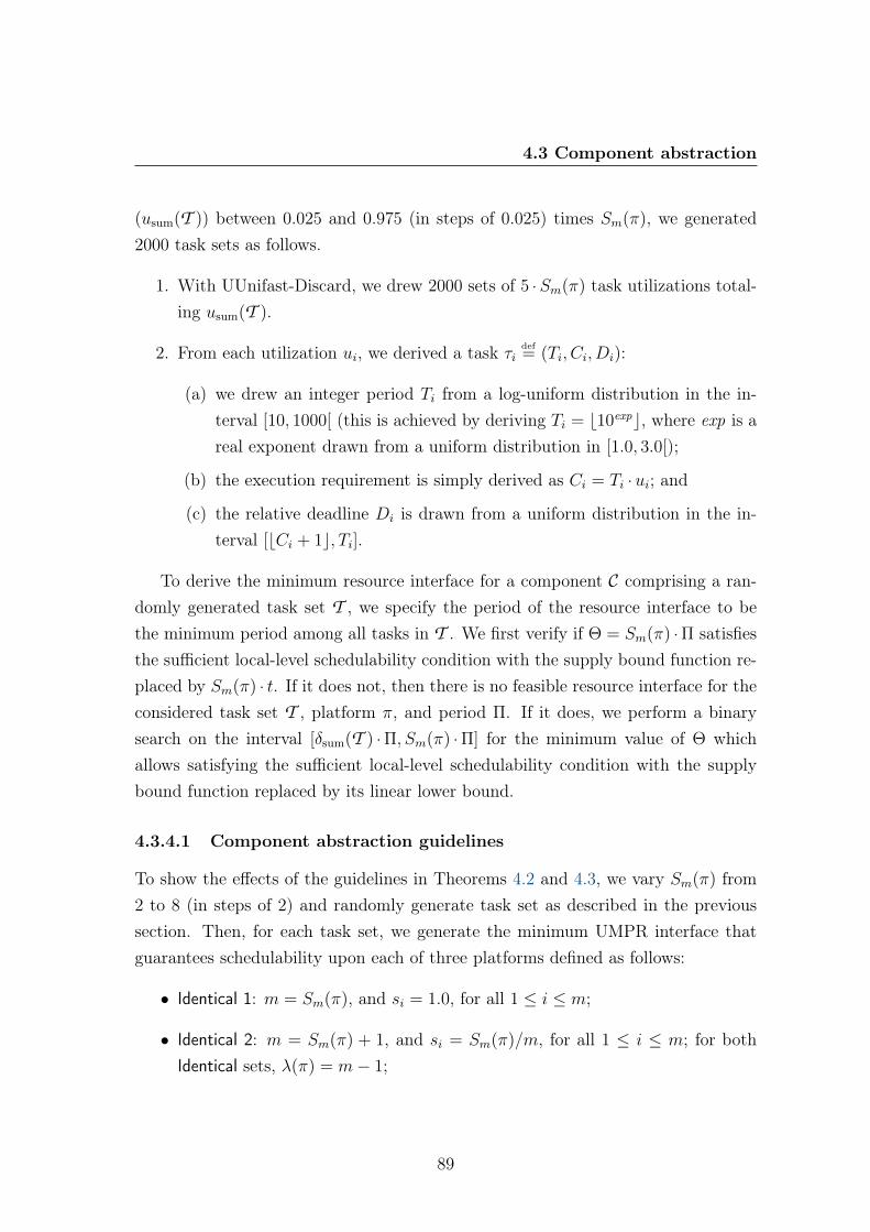
4.3 Component abstraction

(usum(T )) between 0.025 and 0.975 (in steps of 0.025) times Sm(π), we generated2000 task sets as follows.

1. With UUnifast-Discard, we drew 2000 sets of 5 ·Sm(π) task utilizations total-ing usum(T ).

2. From each utilization ui, we derived a task τidef= (Ti, Ci, Di):

(a) we drew an integer period Ti from a log-uniform distribution in the in-terval [10, 1000[ (this is achieved by deriving Ti = b10expc, where exp is areal exponent drawn from a uniform distribution in [1.0, 3.0[);

(b) the execution requirement is simply derived as Ci = Ti ·ui; and

(c) the relative deadline Di is drawn from a uniform distribution in the in-terval [bCi + 1c, Ti].

To derive the minimum resource interface for a component C comprising a ran-domly generated task set T , we specify the period of the resource interface to bethe minimum period among all tasks in T . We first verify if Θ = Sm(π) · Π satisfiesthe sufficient local-level schedulability condition with the supply bound function re-placed by Sm(π) · t. If it does not, then there is no feasible resource interface for theconsidered task set T , platform π, and period Π. If it does, we perform a binarysearch on the interval [δsum(T ) · Π, Sm(π) · Π] for the minimum value of Θ whichallows satisfying the sufficient local-level schedulability condition with the supplybound function replaced by its linear lower bound.

4.3.4.1 Component abstraction guidelines

To show the effects of the guidelines in Theorems 4.2 and 4.3, we vary Sm(π) from2 to 8 (in steps of 2) and randomly generate task set as described in the previoussection. Then, for each task set, we generate the minimum UMPR interface thatguarantees schedulability upon each of three platforms defined as follows:

• Identical 1: m = Sm(π), and si = 1.0, for all 1 ≤ i ≤ m;

• Identical 2: m = Sm(π) + 1, and si = Sm(π)/m, for all 1 ≤ i ≤ m; for bothIdentical sets, λ(π) = m− 1;

89

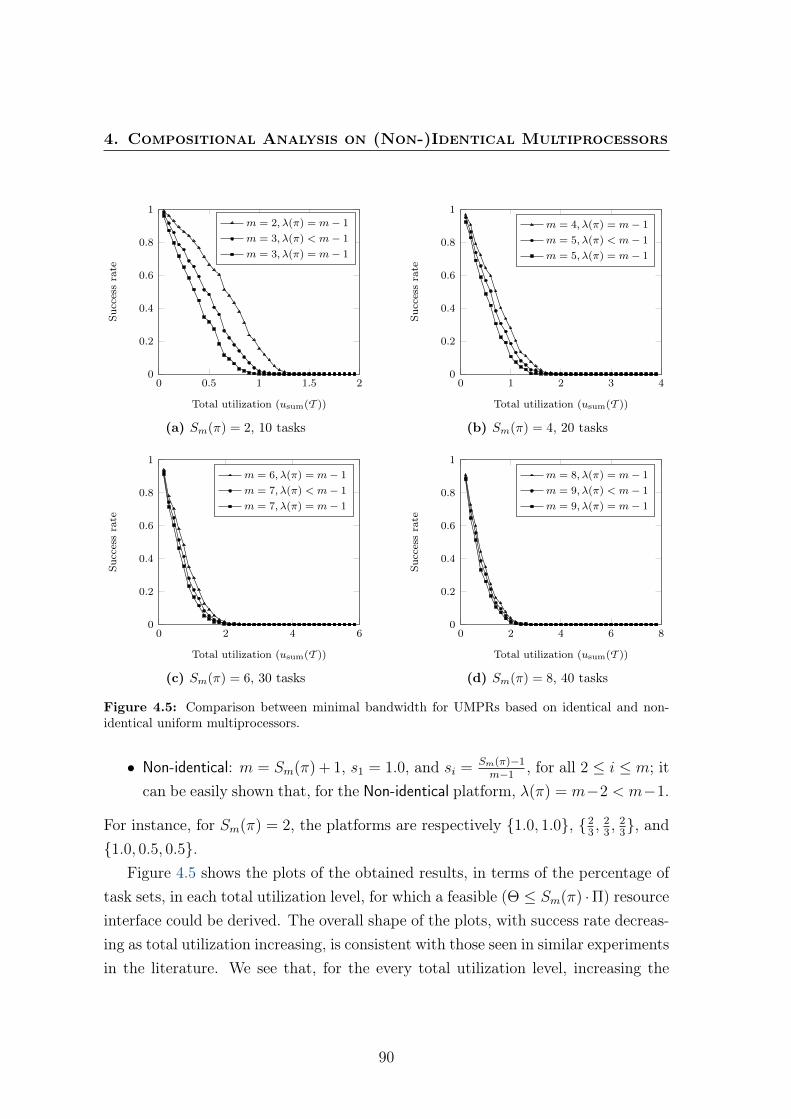
4. Compositional Analysis on (Non-)Identical Multiprocessors

0 0.5 1 1.5 20

0.2

0.4

0.6

0.8

1

Total utilization (usum(T ))

Successrate

m = 2, λ(π) = m− 1

m = 3, λ(π) < m− 1

m = 3, λ(π) = m− 1

(a) Sm(π) = 2, 10 tasks

0 1 2 3 40

0.2

0.4

0.6

0.8

1

Total utilization (usum(T ))Su

ccessrate

m = 4, λ(π) = m− 1

m = 5, λ(π) < m− 1

m = 5, λ(π) = m− 1

(b) Sm(π) = 4, 20 tasks

0 2 4 60

0.2

0.4

0.6

0.8

1

Total utilization (usum(T ))

Successrate

m = 6, λ(π) = m− 1

m = 7, λ(π) < m− 1

m = 7, λ(π) = m− 1

(c) Sm(π) = 6, 30 tasks

0 2 4 6 80

0.2

0.4

0.6

0.8

1

Total utilization (usum(T ))

Successrate

m = 8, λ(π) = m− 1

m = 9, λ(π) < m− 1

m = 9, λ(π) = m− 1

(d) Sm(π) = 8, 40 tasks

Figure 4.5: Comparison between minimal bandwidth for UMPRs based on identical and non-identical uniform multiprocessors.

• Non-identical: m = Sm(π) + 1, s1 = 1.0, and si = Sm(π)−1m−1

, for all 2 ≤ i ≤ m; itcan be easily shown that, for the Non-identical platform, λ(π) = m−2 < m−1.

For instance, for Sm(π) = 2, the platforms are respectively {1.0, 1.0}, {23, 2

3, 2

3}, and

{1.0, 0.5, 0.5}.Figure 4.5 shows the plots of the obtained results, in terms of the percentage of

task sets, in each total utilization level, for which a feasible (Θ ≤ Sm(π) · Π) resourceinterface could be derived. The overall shape of the plots, with success rate decreas-ing as total utilization increasing, is consistent with those seen in similar experimentsin the literature. We see that, for the every total utilization level, increasing the

90

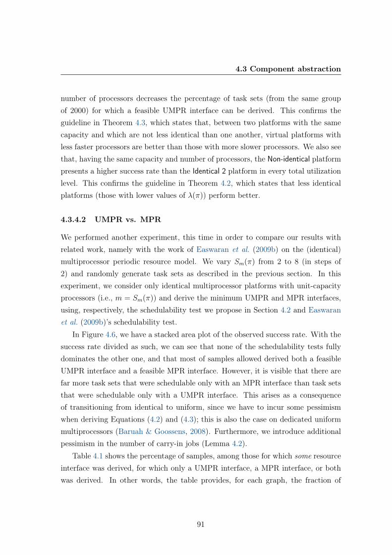
4.3 Component abstraction

number of processors decreases the percentage of task sets (from the same groupof 2000) for which a feasible UMPR interface can be derived. This confirms theguideline in Theorem 4.3, which states that, between two platforms with the samecapacity and which are not less identical than one another, virtual platforms withless faster processors are better than those with more slower processors. We also seethat, having the same capacity and number of processors, the Non-identical platformpresents a higher success rate than the Identical 2 platform in every total utilizationlevel. This confirms the guideline in Theorem 4.2, which states that less identicalplatforms (those with lower values of λ(π)) perform better.

4.3.4.2 UMPR vs. MPR

We performed another experiment, this time in order to compare our results withrelated work, namely with the work of Easwaran et al. (2009b) on the (identical)multiprocessor periodic resource model. We vary Sm(π) from 2 to 8 (in steps of2) and randomly generate task sets as described in the previous section. In thisexperiment, we consider only identical multiprocessor platforms with unit-capacityprocessors (i.e., m = Sm(π)) and derive the minimum UMPR and MPR interfaces,using, respectively, the schedulability test we propose in Section 4.2 and Easwaranet al. (2009b)’s schedulability test.

In Figure 4.6, we have a stacked area plot of the observed success rate. With thesuccess rate divided as such, we can see that none of the schedulability tests fullydominates the other one, and that most of samples allowed derived both a feasibleUMPR interface and a feasible MPR interface. However, it is visible that there arefar more task sets that were schedulable only with an MPR interface than task setsthat were schedulable only with a UMPR interface. This arises as a consequenceof transitioning from identical to uniform, since we have to incur some pessimismwhen deriving Equations (4.2) and (4.3); this is also the case on dedicated uniformmultiprocessors (Baruah & Goossens, 2008). Furthermore, we introduce additionalpessimism in the number of carry-in jobs (Lemma 4.2).

Table 4.1 shows the percentage of samples, among those for which some resourceinterface was derived, for which only a UMPR interface, a MPR interface, or bothwas derived. In other words, the table provides, for each graph, the fraction of

91

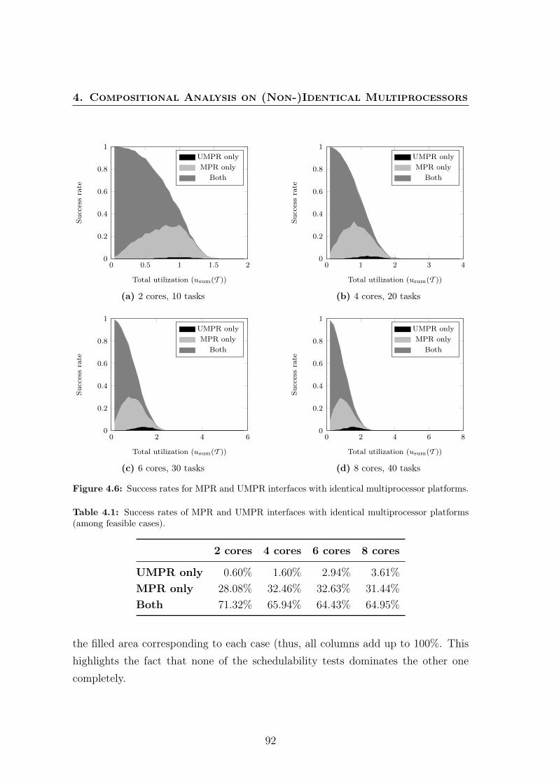
4. Compositional Analysis on (Non-)Identical Multiprocessors

0 0.5 1 1.5 20

0.2

0.4

0.6

0.8

1

Total utilization (usum(T ))

Successrate

UMPR onlyMPR only

Both

(a) 2 cores, 10 tasks

0 1 2 3 40

0.2

0.4

0.6

0.8

1

Total utilization (usum(T ))

Successrate

UMPR onlyMPR only

Both

(b) 4 cores, 20 tasks

0 2 4 60

0.2

0.4

0.6

0.8

1

Total utilization (usum(T ))

Successrate

UMPR onlyMPR only

Both

(c) 6 cores, 30 tasks

0 2 4 6 80

0.2

0.4

0.6

0.8

1

Total utilization (usum(T ))

Successrate

UMPR onlyMPR only

Both

(d) 8 cores, 40 tasks

Figure 4.6: Success rates for MPR and UMPR interfaces with identical multiprocessor platforms.

Table 4.1: Success rates of MPR and UMPR interfaces with identical multiprocessor platforms(among feasible cases).

2 cores 4 cores 6 cores 8 cores

UMPR only 0.60% 1.60% 2.94% 3.61%

MPR only 28.08% 32.46% 32.63% 31.44%

Both 71.32% 65.94% 64.43% 64.95%

the filled area corresponding to each case (thus, all columns add up to 100%. Thishighlights the fact that none of the schedulability tests dominates the other onecompletely.

92

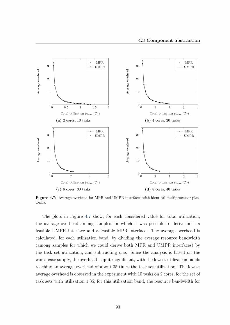
4.3 Component abstraction

0 0.5 1 1.5 20

10

20

30

Total utilization (usum(T ))

Average

overhead

MPRUMPR

(a) 2 cores, 10 tasks

0 1 2 3 40

10

20

30

Total utilization (usum(T ))

Average

overhead

MPRUMPR

(b) 4 cores, 20 tasks

0 2 4 60

10

20

30

Total utilization (usum(T ))

Average

overhead

MPRUMPR

(c) 6 cores, 30 tasks

0 2 4 6 80

10

20

30

Total utilization (usum(T ))

Average

overheadMPRUMPR

(d) 8 cores, 40 tasks

Figure 4.7: Average overhead for MPR and UMPR interfaces with identical multiprocessor plat-forms.

The plots in Figure 4.7 show, for each considered value for total utilization,the average overhead among samples for which it was possible to derive both afeasible UMPR interface and a feasible MPR interface. The average overhead iscalculated, for each utilization band, by dividing the average resource bandwidth(among samples for which we could derive both MPR and UMPR interfaces) bythe task set utilization, and subtracting one. Since the analysis is based on theworst-case supply, the overhead is quite significant, with the lowest utilization bandsreaching an average overhead of about 35 times the task set utilization. The lowestaverage overhead is observed in the experiment with 10 tasks on 2 cores, for the set oftask sets with utilization 1.35; for this utilization band, the resource bandwidth for

93

4. Compositional Analysis on (Non-)Identical Multiprocessors

MPR and UMPR interfaces is, respectively, 38% and 42% greater (on average) thanthe task set utilization. Contrarily to this particular data point, in most experimentsand utilization values the UMPR interfaces presents less overhead that the MPRinterfaces.

4.4 Intercomponent scheduling

We first approach the problem of interface composition assuming that C0 is the rootcomponent of the system (i.e., has access to a dedicated uniform multiprocessorplatform). The resulting interface composition is also appliable to situations whereC0 is not the root component, albeit resulting in a pessimistic resource interface U0.At the end of this section, we present improvements for this scenario.

We consider the system model we presented in Section 3.3, which we now brieflyrestate. Component C0 has q children components Cp (1 ≤ p ≤ q), comprisinga scheduling algorithm Ap = gEDF to schedule task set Tp

def= {τp,i}npi=1. Each

component Cp has a UMPR resource interface Updef= (Πp,Θp, πp), which abstracts:

• to C0, the overall resource demand Cp requires; and

• to Cp, the resource supply that C0 provides.

The virtual platform in the resource interface, πpdef= {sp,j}mpj=1, is a uniform multi-

processor platform.

4.4.1 Transforming components to interface tasks

As we have mentioned in Section 4.1, deriving a task set with an execution require-ment equivalent to that of a component allows scheduling with a traditional sched-uler (such as gEDF) and possibly analysis with classical results. We now present amethod of transforming a UMPR interface Up into a set of mp periodic tasks. Aperiodic task is a particular case of a sporadic task whose jobs have their arrivaltimes exactly separated by fixed time interval— the task’s period.

Consider a UMPR interface Up = (Πp,Θp, πp). Let us have

bdef= Θp − Smp(πp) ·

⌊Θp

Smp(πp)

⌋and k

def= max {` : S`(πp) ≤ b} .

94

4.4 Intercomponent scheduling

We define the transformation from Up to a periodic task set T (Up) with mp tasksτ

(Up)i

def= (T

(Up)i , C

(Up)i , D

(Up)i ) such that:

• if i ≤ k, τ (Up)i =

(Πp,(⌊

ΘpSmp (πp)

⌋+ 1)

· sp,i,Πp

);

• if i = k + 1, τ (Up)i =

(Πp,⌊

ΘpSmp (πp)

⌋· sp,i + b− Sk(πp),Πp

);

• otherwise, τ (Up)i =

(Πp,⌊

ΘpSmp (πp)

⌋· sp,i,Πp

).

Theorem 4.4 (Generalization of the task transformation for the MPR). Considerthe UMPR Up = (Πp,Θp, πp). If πp is in fact an identical multiprocessor platform,this transformation becomes equivalent to that by Easwaran et al. (2009b) for theMPR model.

Proof. If πp is an mp-processor identical multiprocessor platform, then all processorshave speed 1.0, and S`(πp) = `, for all ` ≤ mp. Hence, b

def= Θp−Smp(πp) ·

⌊Θp

Smp (πp)

⌋=

Θp −mp ·⌊

Θmp

⌋and k def

= max {` : S`(πp) ≤ b} = max {` ∈ N : ` ≤ b} = bbc. Thesematch the definitions by Easwaran et al. (2009b) (see Section 2.4.3.1). When wereplace Smp(πp) with mp and all sp,i’s with 1 in the definition of our transformation,we have the following rules:

• if i ≤ k, τ (Up)i =

(Πp,⌊

Θpmp

⌋+ 1),Πp

);

• if i = k+1, τ (Up)i =

(Πp,⌊

Θpmp

⌋+ b− Sk(π),Πp

)=(

Πp,⌊

Θpmp

⌋+ b− k ·

⌊bk

⌋,Πp

);

• otherwise, τ (Up)i =

(Πp,⌊

Θpmp

⌋,Πp

);

which match the rules of the transformation from MPR to tasks presented byEaswaran et al. (2009b). �

Lemma 4.7. The sum of the execution requirements of all the tasks in T (Up) isequal to Θp.

Proof. To prove this lemma, we consider three separate cases:

1. Θp is exactly divisible by Smp(πp);

2. Θp is not exactly divisible by Smp(πp), and Sk(πp) = b; or

95

4. Compositional Analysis on (Non-)Identical Multiprocessors

3. Θp is not exactly divisible by Smp(πp), and Sk(πp) < b.

Case 1. If Θp is exactly divisible by Smp(πp), then b = 0 and k = 0. Hence, T (Up)

will have:

• one task (τ (Up)1

def= τ

(Up)k+1 ) with execution requirement

⌊Θp

Smp (πp)

⌋· sp,i + b −

Sk(πp) = ΘpSmp (πp)

· sp,i, with i = 1; and

• mp − 1 tasks, each with execution requirement⌊

ΘpSmp (πp)

⌋· sp,i = Θp

Smp (πp)· sp,i,

with i ∈ [2..mp].

The total execution requirement is given by

∑τ

(Up)

i ∈T (Up)

C(Up)i =

mp∑i=1

Θp

Smp(πp)· sp,i

=Θp

Smp(πp)·mp∑i=1

sp,i

=Θp

Smp(πp)·Smp(πp)

= Θp .

Case 2. If Θp is not exactly divisible by Smp(πp), then b > 0. Let us consider thatk is such that Sk(πp) = b (therefore, k > 0). Hence, T (Up) will have:

• k tasks with execution requirement(⌊

ΘpSmp (πp)

⌋+ 1)

· sp,i, with i ∈ [1..k];

• one task with execution requirement⌊

ΘpSmp (πp)

⌋· sp,i+b−Sk(πp) =

⌊Θp

Smp (πp)

⌋· sp,i,

with i = k + 1; and

• mp − (k + 1) tasks with execution requirement⌊

ΘpSmp (πp)

⌋· sp,i,

with i ∈ [k + 2 ..mp].

96

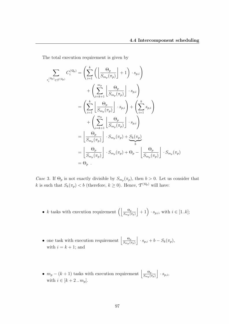
4.4 Intercomponent scheduling

The total execution requirement is given by

∑τ

(Up)

i ∈T (Up)

C(Up)i =

(k∑i=1

(⌊Θp

Smp(πp)

⌋+ 1

)· sp,i

)

+

(mp∑

i=k+1

⌊Θp

Smp(πp)

⌋· sp,i

)

=

(k∑i=1

⌊Θp

Smp(πp)

⌋· sp,i

)+

(k∑i=1

sp,i

)

+

(mp∑

i=k+1

⌊Θp

Smp(πp)

⌋· sp,i

)

=

⌊Θp

Smp(πp)

⌋·Smp(πp) + Sk(πp)︸ ︷︷ ︸

b

=

⌊Θp

Smp(πp)

⌋·Smp(πp) + Θp −

⌊Θp

Smp(πp)

⌋·Smp(πp)

= Θp .

Case 3. If Θp is not exactly divisible by Smp(πp), then b > 0. Let us consider thatk is such that Sk(πp) < b (therefore, k ≥ 0). Hence, T (Up) will have:

• k tasks with execution requirement(⌊

ΘpSmp (πp)

⌋+ 1)

· sp,i, with i ∈ [1..k];

• one task with execution requirement⌊

ΘpSmp (πp)

⌋· sp,i + b− Sk(πp),

with i = k + 1; and

• mp − (k + 1) tasks with execution requirement⌊

ΘpSmp (πp)

⌋· sp,i,

with i ∈ [k + 2 ..mp].

97

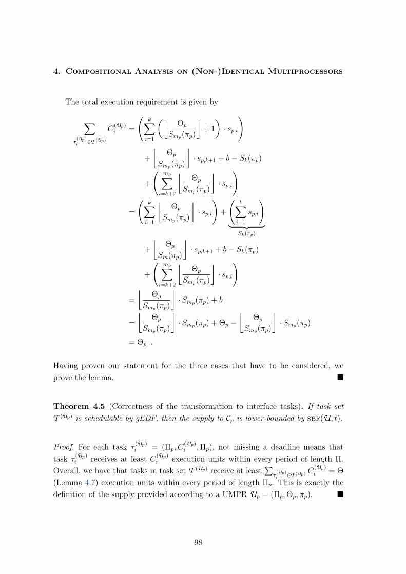
4. Compositional Analysis on (Non-)Identical Multiprocessors

The total execution requirement is given by

∑τ

(Up)

i ∈T (Up)

C(Up)i =

(k∑i=1

(⌊Θp

Smp(πp)

⌋+ 1

)· sp,i

)

+

⌊Θp

Smp(πp)

⌋· sp,k+1 + b− Sk(πp)

+

(mp∑

i=k+2

⌊Θp

Smp(πp)

⌋· sp,i

)

=

(k∑i=1

⌊Θp

Smp(πp)

⌋· sp,i

)+

(k∑i=1

sp,i

)︸ ︷︷ ︸

Sk(πp)

+

⌊Θp

Sm(πp)

⌋· sp,k+1 + b− Sk(πp)

+

(mp∑

i=k+2

⌊Θp

Smp(πp)

⌋· sp,i

)

=

⌊Θp

Smp(πp)

⌋·Smp(πp) + b

=

⌊Θp

Smp(πp)

⌋·Smp(πp) + Θp −

⌊Θp

Smp(πp)

⌋·Smp(πp)

= Θp .

Having proven our statement for the three cases that have to be considered, weprove the lemma. �

Theorem 4.5 (Correctness of the transformation to interface tasks). If task setT (Up) is schedulable by gEDF, then the supply to Cp is lower-bounded by sbf(U, t).

Proof. For each task τ(Up)i = (Πp, C

(Up)i ,Πp), not missing a deadline means that

task τ (Up)i receives at least C(Up)

i execution units within every period of length Π.Overall, we have that tasks in task set T (Up) receive at least

∑τ

(Up)

i ∈T (Up) C(Up)i = Θ

(Lemma 4.7) execution units within every period of length Πp. This is exactly thedefinition of the supply provided according to a UMPR Up = (Πp,Θp, πp). �

98

4.4 Intercomponent scheduling

4.4.2 Compositionality with gEDF intercomponent schedul-ing

Let us have component C1, which is schedulable with the smallest possible band-width with UMPR interface U1 = (Π1,Θ1, π1), where π1 = {v, w, y} such that1.0 ≥ v = w > y > 0.0. Now let us assume that, with consideration to the re-maining components, we employ a physical platform π0 = {v, w, x, y} such that1.0 ≥ v = w = x > y > 0.0. To schedule C1, gEDF will schedule the respectiveinterface tasks— τ

(U1)1 , τ (U1)

2 , and τ(U1)3 —on the available processors. The exact

processors upon which C1’s interface tasks are scheduled depend on competitionwith the interface tasks of the remaining components. In the extreme case, C1’sinterface tasks may be always scheduled on the three fastest processors in the plat-form. This means C1 ends up receiving resource according to a different UMPRinterface, U ′1 = (Π1,Θ1, π

′1), where π′1 = {v, w, x} such that 1.0 ≥ v = w = x > 0.0.

We now prove two lemmas to show the impact of this scenario on the schedulabilityof C1.

Lemma 4.8. For any values of v, w, x, y such that 1.0 ≥ v = w = x > y > 0.0,λ(π′1) > λ(π1).

Proof. We prove this by contradiction; assume λ(π′1) ≤ λ(π1). By definition, thismeans

max

{w + x

v,x

w

}≤ max

{w + y

v,y

w

}.

Since v = w, we can replace all occurrences of v with w and rearrange, and have

max{ xw

+ 1,x

w

}≤ max

{ yw

+ 1,y

w

}x

w+ 1 ≤ y

w+ 1

x ≤ y ,

which contradicts the assumption that x > y. �

Lemma 4.9. If C1 receives resource according to U ′1 (instead of U1), it is notguaranteed to be able schedule its tasks.

99

4. Compositional Analysis on (Non-)Identical Multiprocessors

Proof. Since U1 schedules C1 with the smallest possible bandwidth, then, by defini-tion, for some task τk and some Ak ≥ 0,∑

τi∈T

dbf(τi, Ak +Dk) + (ν + λ(π1)) · (Ak +Dk) · δmax(T ) = lsbf(U1, Ak +Dk) .

For the same τk and Ak, since λ(π′1) > λ(π1) (Lemma 4.8), we have∑τi∈T

dbf(τi, Ak +Dk) + (ν + λ(π′1)) · (Ak +Dk) · δmax(T )

>∑τi∈T

dbf(τi, Ak +Dk) + (ν + λ(π1)) · (Ak +Dk) · δmax(T ) .

On the other hand, since Sm(π′1) > Sm(π), lsbf(U ′1, t) < lsbf(U1, t) (for all valuesof t > 0), i.e.,

lsbf(U1, Ak +Dk) > lsbf(U ′1, Ak +Dk) .

Consequently,∑τi∈T

dbf(τi, Ak +Dk) + (ν + λ(π′1)) · (Ak +Dk) · δmax(T ) > lsbf(U ′1, Ak +Dk) ,

which means U ′1 cannot guarantee schedulability of the tasks in component C1. �

Having proven these two lemmas, we can now prove an important theorem.

Theorem 4.6 (Inadequacy of gEDF for intercomponent scheduling). If A0 is gEDF,the considered scheduling framework (Figure 4.1) is not compositional.

Proof. This follows from our example and Lemma 4.9. We cannot guarantee that theproperties established and validated for components in isolation (namely, schedula-bility) hold once the components are integrated to form the system. �

We have been able to show the inadequacy of gEDF as an intercomponent

scheduling algorithm in the presence of different types of processors.

100

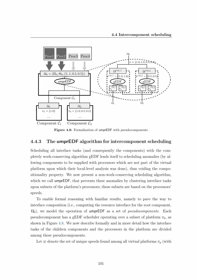
4.4 Intercomponent scheduling

umprEDF

U1

Component C0

Component C2Component C1

Proc3 Proc4

π1 = {1.0}

U2

π2 = {1.0, 0.5, 0.5}

U ($1) U ($2)

gEDF gEDF

τ(U2)1 τ

(U2)2 τ

(U2)3τ

(U1)1

π($1) = {1.0, 1.0} π($2) = {0.5, 0.5}

U1 U2

U0

U0 = (Π0,Θ0, {1, 1, 0.5, 0.5})

... ...

π = {1.0, 1.0, 0.5, 0.5}

Proc1 Proc2

Figure 4.8: Formalization of umprEDF with pseudocomponents

4.4.3 The umprEDF algorithm for intercomponent scheduling

Scheduling all interface tasks (and consequently the components) with the com-pletely work-conserving algorithm gEDF lends itself to scheduling anomalies (by al-lowing components to be supplied with processors which are not part of the virtualplatform upon which their local-level analysis was done), thus voiding the compo-sitionality property. We now present a non-work-conserving scheduling algorithm,which we call umprEDF, that prevents these anomalies by clustering interface tasksupon subsets of the platform’s processors; these subsets are based on the processors’speeds.

To enable formal reasoning with familiar results, namely to pave the way tointerface composition (i.e., computing the resource interface for the root component,U0), we model the operation of umprEDF as a set of pseudocomponents. Eachpseudocomponent has a gEDF scheduler operating over a subset of platform π0, asshown in Figure 4.8. We now describe formally and in more detail how the interfacetasks of the children components and the processors in the platform are dividedamong these pseudocomponents.

Let $ denote the set of unique speeds found among all virtual platforms πp (with

101

4. Compositional Analysis on (Non-)Identical Multiprocessors

1 ≤ p ≤ q). For each $` ∈ $, we assume a pseudocomponent C($`) aggregating allthe tasks which model the contribution of processors with speed $`. Formally:

T ($`) def=⋃p≤q

{τ

(Up)i ∈ T (Up) | sp,i = $`

}. (4.8)

Lemma 4.10. If the set of interface tasks of component Cp (which is T (Up), definedin Equation (4.8)) is schedulable with umprEDF, then the resource provided to Cp isguaranteed to comply with Up, both in terms of supply and platform.

Proof. We can prove the compliance in terms of supply as we did for gEDF inTheorem 4.5. For each task τ (Up)

i = (Πp, C(Up)i ,Πp), not missing a deadline means

that task τ (Up)i receives at least C(Up)

i execution units within every period of length Π.Overall, we have that tasks in task set T (Up) receive at least

∑τ

(Up)

i ∈T (Up) C(Up)i = Θ

(Lemma 4.7) execution units within every period of length Πp. This is exactly thedefinition of the supply provided according to a UMPR Up = (Πp,Θp, πp).

With respect to the platform, compliance with the component’s resource interfacecomes from the division of the interface tasks in the different pseudocomponents,and from the fact that the interface tasks are paired with the processors consideredin the virtual platform πp. �

The following theorem directly follows from Lemma 4.10.

Theorem 4.7 (Adequacy of umprEDF for intercomponent scheduling). If A0 isumprEDF, the considered scheduling framework (Figure 4.1) is compositional.

4.4.4 Interface composition

We then derive the resource interface for each pseudocomponent C($`) —a UMPRinterface U($`) def

= (Π0,Θ($`), π($`)). Since we are under the assumption that we are

working with the physical platform, the processors in π($`) are all fully available.We just need to compute how many of them we will need and Θ($`) is set to be equalto Π0 ·Sm($`)(π

($`)) (for an arbitrary Π0). For this, we iterate on m($`), consideringeach platform composed of m($`) processors with speed $`, and stopping at theminimum value of m($`) for which T ($`) is schedulable. Since the interface tasks areperiodic, we can use schedulability tests thereto specific, which are less pessimistic.

102

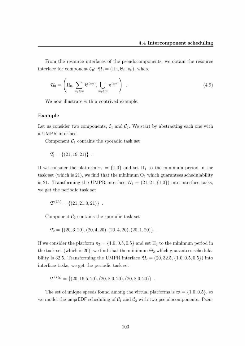
4.4 Intercomponent scheduling

From the resource interfaces of the pseudocomponents, we obtain the resourceinterface for component C0: U0 = (Π0,Θ0, π0), where

U0 =

(Π0,

∑$`∈$

Θ($`),⋃$`∈$

π($`)

). (4.9)

We now illustrate with a contrived example.

Example

Let us consider two components, C1 and C2. We start by abstracting each one witha UMPR interface.

Component C1 contains the sporadic task set

T1 = {(21, 19, 21)} .

If we consider the platform π1 = {1.0} and set Π1 to the minimum period in thetask set (which is 21), we find that the minimum Θ1 which guarantees schedulabilityis 21. Transforming the UMPR interface U1 = (21, 21, {1.0}) into interface tasks,we get the periodic task set

T (U1) = {(21, 21.0, 21)} .

Component C2 contains the sporadic task set

T2 = {(20, 3, 20), (20, 4, 20), (20, 4, 20), (20, 1, 20)} .

If we consider the platform π2 = {1.0, 0.5, 0.5} and set Π2 to the minimum period inthe task set (which is 20), we find that the minimum Θ2 which guarantees schedula-bility is 32.5. Transforming the UMPR interface U2 = (20, 32.5, {1.0, 0.5, 0.5}) intointerface tasks, we get the periodic task set

T (U2) = {(20, 16.5, 20), (20, 8.0, 20), (20, 8.0, 20)} .

The set of unique speeds found among the virtual platforms is $ = {1.0, 0.5}, sowe model the umprEDF scheduling of C1 and C2 with two pseudocomponents. Pseu-

103

4. Compositional Analysis on (Non-)Identical Multiprocessors

docomponent C($1) contains the interface tasks τ (U1)1 = (21, 21.0, 21) and τ

(U2)1 =

(20, 16.5, 20). Conversely, pseudocomponent C($2) contains the interface tasks τ (U2)2 =

(20, 8.0, 20), and τ (U2)3 = (20, 8.0, 20). Since these are periodic tasks being scheduled

upon a dedicated uniform multiprocessor platform, we can use the exact test derivedby Funk et al. (2001). According to this test, a periodic task set is gEDF-schedulableon a uniform multiprocessor platform with m processors if and only if

• the total utilization of the task set does not exceed the total capacity of theplatform; and

• for all k = 1, . . . ,m, the sum of the k higher utilizations in the task set doesnot exceed the sum of the capacities of the k fastest processors in the platform.

With this test, we can assess that pseudocomponent C($1) needs two unit-capacityprocessors to guarantee schedulability, whereas pseudocomponent C($2) needs two0.5-capacity processors.

If we select a value of Π0 = 20, then the UMPR interfaces of the pseudocom-ponents are U($1) = (20, 40, {1.0, 1.0}) and U($2) = (20, 20, {0.5, 0.5}). ApplyingEquation (4.9), we obtain the UMPR interface for C0:

U0 = (20, 60, {1.0, 1.0, 0.5, 0.5}) ,

which corresponds to a dedicated availability of platform π0 = {1.0, 1.0, 0.5, 0.5}.Although in this example the platform π0 is identical to the union of all the virtualplatforms, it is possible that it is a subset of this union (formally, π0 ⊆

⋃qp=1 πp), as

seen in Figure 4.1.

4.5 Summary

We approached the problem of compositional analysis upon uniform multiprocessorplatforms, proposing the Uniform Multiprocessor Resource (UMPR) model to ex-press component interfaces. We extended previous related works, providing resultsand intuitions which span over the three main points of compositional analysis:

• a sufficient local-level gEDF-schedulability test for sporadic task sets in com-ponents with the UMPR as a resource interface;

104

4.5 Summary

• guidelines for the complex problem of selecting the virtual platform whenabstracting a component; and

• interface composition based on a new intercomponent scheduling algorithm,umprEDF, that solves the inadequacy of using gEDF to schedule componentswith non-identical multiprocessor virtual platforms.

We do still have room for improvement of these results. We envision providing aquantitative evaluation—with some resource augmentation-based (Phillips et al.,2002) metric—of the UMPR and related theoretical results, as well as tighteningthe latter to reduce the incurred pessimism and overhead. Furthermore, we intendto assess the potential for other models built upon identical multiprocessors (e.g.,Lipari & Bini (2010)’s) to be extended to deal with uniform multiprocessor platforms(albeit with a different compromise between simplicity and bandwidth optimality).

In the next chapter, we present the design, development and use of a proof-of-concept analysis and simulation tool where the formal methods proposed in thischapter can be seen in action. Our tool also allows generating a partition schedulingtable to configure systems based on a cyclic partition scheduler, such as those basedon the evolved TSP architecture presented in Chapter 3.

105

Chapter 5

Scheduling Analysis, Generationand Simulation Tool

In this chapter, we describe the design, development and use of hsSim, an extensibleand interoperable tool that allows analyzing and simulating hierarchically organizedmultiprocessor real-time systems (such as hierarchical scheduling and resource reser-vation frameworks), as well as generating partition scheduling tables for the specificcase of TSP systems. From the beginning, we imprinted into the development ofhsSim some concerns that have echo in the embedded and real-time systems researchcommunity (Lipari, 2012). For this reason, we put a significant amount of emphasison designing our tool to be easily extended and to interoperate with other tools.In Section 5.1, we describe the analysis and design process, focused on applyingsoftware design patterns to model specific structures and behaviors of real-time sys-tems. In Section 5.2, we describe the implementation of this design. In Section 5.3,we demonstrate our implementations compositional analysis, scheduling simulation(with visualization through the Grasp Player), and scheduling table generation.

5.1 Object-oriented analysis and design

The implementation of a tool which we want to be flexible, extensible and moreeasily maintainable must be preceded by careful analysis and design. We will nowdocument the main analysis and design steps and decisions taken, supported byUnified Modelling Language (UML) diagrams where deemed necessary.

107

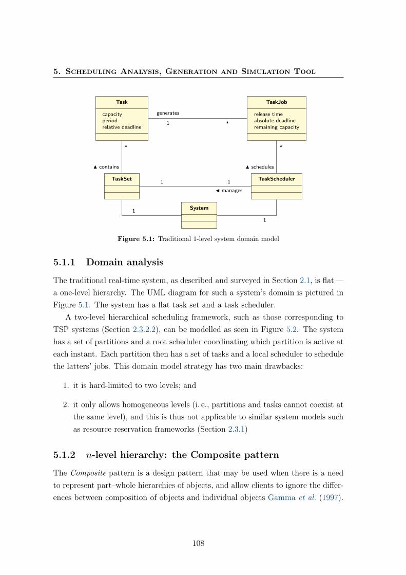
5. Scheduling Analysis, Generation and Simulation Tool

generates

1 *

J manages

11

N contains

*

N schedules

*

1

1

Task

capacityperiodrelative deadline

TaskSet

System

TaskJob

release timeabsolute deadlineremaining capacity

TaskScheduler

Figure 5.1: Traditional 1-level system domain model

5.1.1 Domain analysis

The traditional real-time system, as described and surveyed in Section 2.1, is flat—a one-level hierarchy. The UML diagram for such a system’s domain is pictured inFigure 5.1. The system has a flat task set and a task scheduler.

A two-level hierarchical scheduling framework, such as those corresponding toTSP systems (Section 2.3.2.2), can be modelled as seen in Figure 5.2. The systemhas a set of partitions and a root scheduler coordinating which partition is active ateach instant. Each partition then has a set of tasks and a local scheduler to schedulethe latters’ jobs. This domain model strategy has two main drawbacks:

1. it is hard-limited to two levels; and

2. it only allows homogeneous levels (i. e., partitions and tasks cannot coexist atthe same level), and this is thus not applicable to similar system models suchas resource reservation frameworks (Section 2.3.1)

5.1.2 n-level hierarchy: the Composite pattern

The Composite pattern is a design pattern that may be used when there is a needto represent part–whole hierarchies of objects, and allow clients to ignore the differ-ences between composition of objects and individual objects Gamma et al. (1997).

108

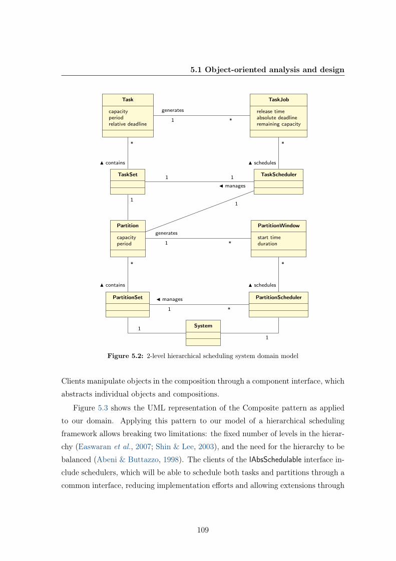
5.1 Object-oriented analysis and design

generates

1 *

J manages

1 *

N contains

*

N schedules

*

1

1

generates

1 *

J manages

11

N contains

*

N schedules

*

11

Partition

capacityperiod

PartitionSet

System

PartitionWindow

start timeduration

PartitionScheduler

Task

capacityperiodrelative deadline

TaskSet

TaskJob

release timeabsolute deadlineremaining capacity

TaskScheduler

Figure 5.2: 2-level hierarchical scheduling system domain model

Clients manipulate objects in the composition through a component interface, which

abstracts individual objects and compositions.

Figure 5.3 shows the UML representation of the Composite pattern as applied

to our domain. Applying this pattern to our model of a hierarchical scheduling

framework allows breaking two limitations: the fixed number of levels in the hierar-

chy (Easwaran et al., 2007; Shin & Lee, 2003), and the need for the hierarchy to be

balanced (Abeni & Buttazzo, 1998). The clients of the IAbsSchedulable interface in-

clude schedulers, which will be able to schedule both tasks and partitions through a

common interface, reducing implementation efforts and allowing extensions through

109

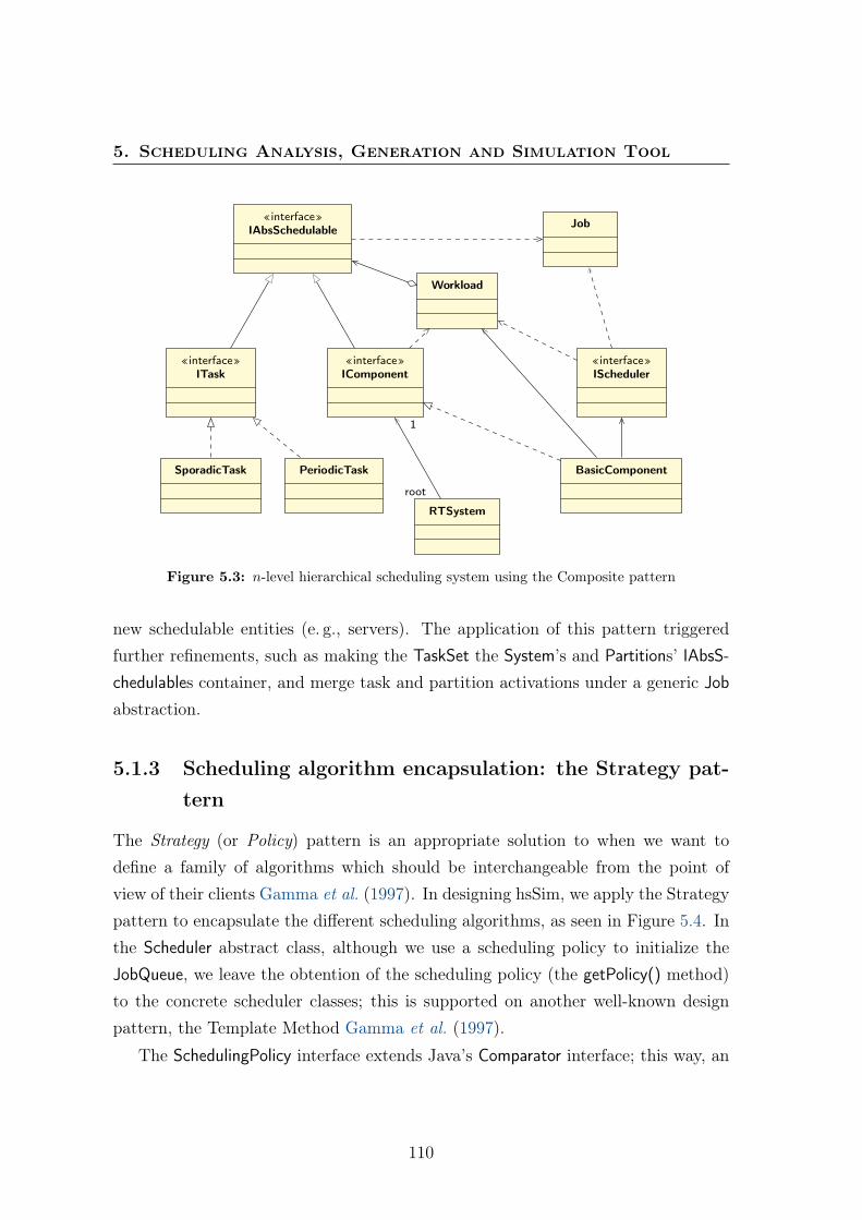
5. Scheduling Analysis, Generation and Simulation Tool

root

1

«interface»IAbsSchedulable

SporadicTask PeriodicTask BasicComponent

RTSystem

«interface»ITask

«interface»IComponent

«interface»IScheduler

Workload

Job

Figure 5.3: n-level hierarchical scheduling system using the Composite pattern

new schedulable entities (e. g., servers). The application of this pattern triggeredfurther refinements, such as making the TaskSet the System’s and Partitions’ IAbsS-chedulables container, and merge task and partition activations under a generic Job

abstraction.

5.1.3 Scheduling algorithm encapsulation: the Strategy pat-tern

The Strategy (or Policy) pattern is an appropriate solution to when we want todefine a family of algorithms which should be interchangeable from the point ofview of their clients Gamma et al. (1997). In designing hsSim, we apply the Strategypattern to encapsulate the different scheduling algorithms, as seen in Figure 5.4. Inthe Scheduler abstract class, although we use a scheduling policy to initialize theJobQueue, we leave the obtention of the scheduling policy (the getPolicy() method)to the concrete scheduler classes; this is supported on another well-known designpattern, the Template Method Gamma et al. (1997).

The SchedulingPolicy interface extends Java’s Comparator interface; this way, an

110

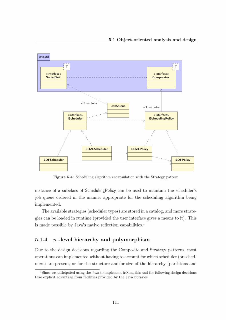
5.1 Object-oriented analysis and design

javautil

«T → Job»«T → Job»

«interface»IScheduler

EDFScheduler

EDZLScheduler

«interface»ISchedulingPolicy

EDZLPolicy

EDFPolicy

JobQueue

«interface»Comparator

T

«interface»SortedSet

T

Figure 5.4: Scheduling algorithm encapsulation with the Strategy pattern

instance of a subclass of SchedulingPolicy can be used to maintain the scheduler’sjob queue ordered in the manner appropriate for the scheduling algorithm beingimplemented.

The available strategies (scheduler types) are stored in a catalog, and more strate-gies can be loaded in runtime (provided the user interface gives a means to it). Thisis made possible by Java’s native reflection capabilities.1

5.1.4 n -level hierarchy and polymorphism

Due to the design decisions regarding the Composite and Strategy patterns, mostoperations can implemented without having to account for which scheduler (or sched-ulers) are present, or for the structure and/or size of the hierarchy (partitions and

1Since we anticipated using the Java to implement hsSim, this and the following design decisionstake explicit advantage from facilities provided by the Java libraries.

111

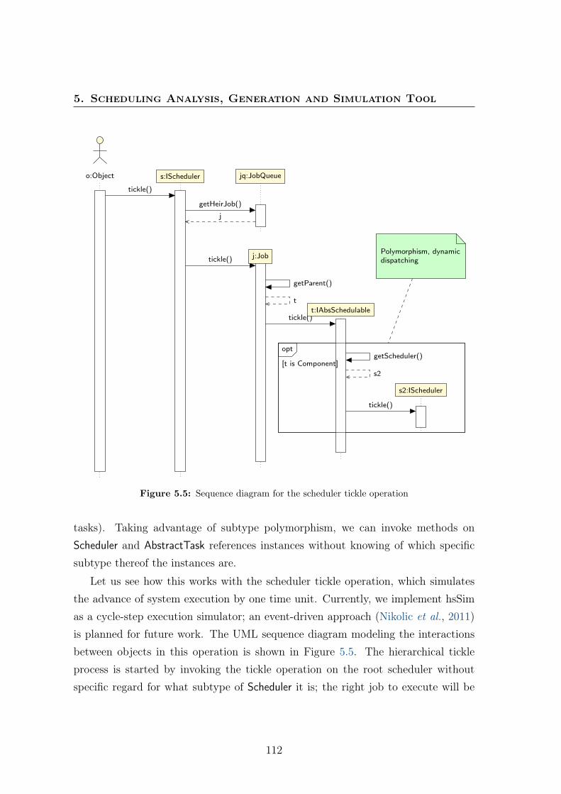
5. Scheduling Analysis, Generation and Simulation Tool

getHeirJob()

j

getParent()

t

getScheduler()

s2

tickle()

tickle()

tickle()

tickle()

o:Object s:IScheduler jq:JobQueue

j:Job

t:IAbsSchedulable

s2:IScheduler

opt

[t is Component]

Polymorphism, dynamicdispatchingPolymorphism, dynamicdispatching

Figure 5.5: Sequence diagram for the scheduler tickle operation

tasks). Taking advantage of subtype polymorphism, we can invoke methods onScheduler and AbstractTask references instances without knowing of which specificsubtype thereof the instances are.

Let us see how this works with the scheduler tickle operation, which simulatesthe advance of system execution by one time unit. Currently, we implement hsSimas a cycle-step execution simulator; an event-driven approach (Nikolic et al., 2011)is planned for future work. The UML sequence diagram modeling the interactionsbetween objects in this operation is shown in Figure 5.5. The hierarchical tickleprocess is started by invoking the tickle operation on the root scheduler withoutspecific regard for what subtype of Scheduler it is; the right job to execute will be

112

5.1 Object-oriented analysis and design

obtained because the scheduler’s job queue is maintained accordingly ordered by aninstance of an unknown SchedulingPolicy subtype. This job is then tickled, and inturns tickles its parent AbstractTask without knowing if it is a Task or a Partition.It is the job’s parent’s responsibility to invoke the right behaviour according to itstype. If it is a Partition instance, this involves tickling its scheduler; this will causean identical chain of polymorphic invocations to take place.

5.1.5 Decoupling the simulation from the simulated domainusing the Observer and Visitor patterns

In hsSim, we want to decouple the simulation aspects (such as running the simulationand logging its occurrences) from the simulated domain itself. On the one hand, wewant changes in the simulated domain (a system with partitions, tasks, jobs) to beexternally known of, namely by one or more loggers, without the domain objectsmaking specific assumptions about these loggers behaviour or interfaces. On theother hand, we want to be able to create new loggers without tightly coupling themto the domain objects or having to modify the latter. We found the Observer andVisitor patterns to be most appropriate to solve this specific problem. In few words,the Observer pattern allows loggers to register themselves as interested in receivingevents, and the Visitor pattern helps each logger define what to do with each kindof event. Let us now see the application of these patterns in detail.

The Observer pattern defines a publisher–subscriber dependency between ob-jects, so that observers (subscribers) are notified automatically of the state changesof the subjects they have subscribed to. The subjects only have to disseminate theirstate changes to a vaguely known set of observers, in a way that is totally indepen-dent of how many observers there are and who they are— in the form of events. Wetake advantage from the simple Observer implementation provided by Java, with theLogger interface extending the Observer interface, as pictured in Figure 5.6. Thisway, classes implementing the Logger interface (the concrete loggers) must providethe method to be called to notify the respective logger of an event.

The Visitor pattern defines a way to represent an operation to be performed onan object hierarchy independently from the latter Gamma et al. (1997). The Loggerinterface also extends our EventVisitor interface, which defines methods to process

113

5. Scheduling Analysis, Generation and Simulation Tool

javautil

observers*

«interface»ILogger

E«interface»Observer

update(o: Observable, arg: Object)

Observable

addObserver(o: Observer)removeObserver(o: Observer)notifyObservers()notifyObservers(arg:Object). . .

notifyObservers(arg)for (Observer o: observers){o.update(this,

arg);}

notifyObservers(arg)for (Observer o: observers){o.update(this,

arg);}

Figure 5.6: Application of the Observer pattern for loggers

«interface»ILogger

E «interface»EventVisitor

visit(JobPreemptedEvent e): Evisit(JobReleasedEvent e): Evisit(JobCompletedEvent e): E. . .

E

JobPreemptedEvent

getPreemptedJob(): JobgetPreemptingJob(): Job. . .

JobReleasedEvent

getJob(): Job. . .

JobCompletedEvent

getJob(): Job. . .

Event

getTime(): int<E> accept(EventVisitor<E> visitor): E

Figure 5.7: Application of the Visitor pattern for loggers

each type of event. The visit methods are overloaded and every Event subclass

114

5.1 Object-oriented analysis and design

*

GEDFScheduler

getPolicy(): ISchedulingPolicy

EDFScheduler

getPolicy(): ISchedulingPolicy

PEDFScheduler

getPolicy(): ISchedulingPolicy

AbsGlobalScheduler

getPolicy(): ISchedulingPolicy

AbsUniprocScheduler

getPolicy(): ISchedulingPolicy

AbsPartScheduler

getPolicy(): ISchedulingPolicy

«interface»IGlobalScheduler

getPolicy(): ISchedulingPolicy

«interface»IUniprocScheduler

getPolicy(): ISchedulingPolicy

«interface»IPartScheduler

getPolicy(): ISchedulingPolicy

«interface»IScheduler

Figure 5.8: Multiprocessor schedulers

provides the following method:

<E> E accept(EventVisitor <E> visitor) {visitor.visit(this);

}

This way, when receiving an event e, a logger only has to invoke

((Event) e). accept(this)

to have the right visit method called.We also apply the Observer pattern to establish a dependency between the sys-

tem clock and the schedulers, so that the latter become aware of when to releasedtheir tasks’ jobs.

5.1.6 Multiprocessor schedulers

As we have seen in Section 2.1.3, the degree of migration that a multiprocessorscheduling algorithm permits to the jobs it schedules allows categorizing it as ei-ther partitioned or global. Uniprocessor schedulers can be seen as a particular case

115

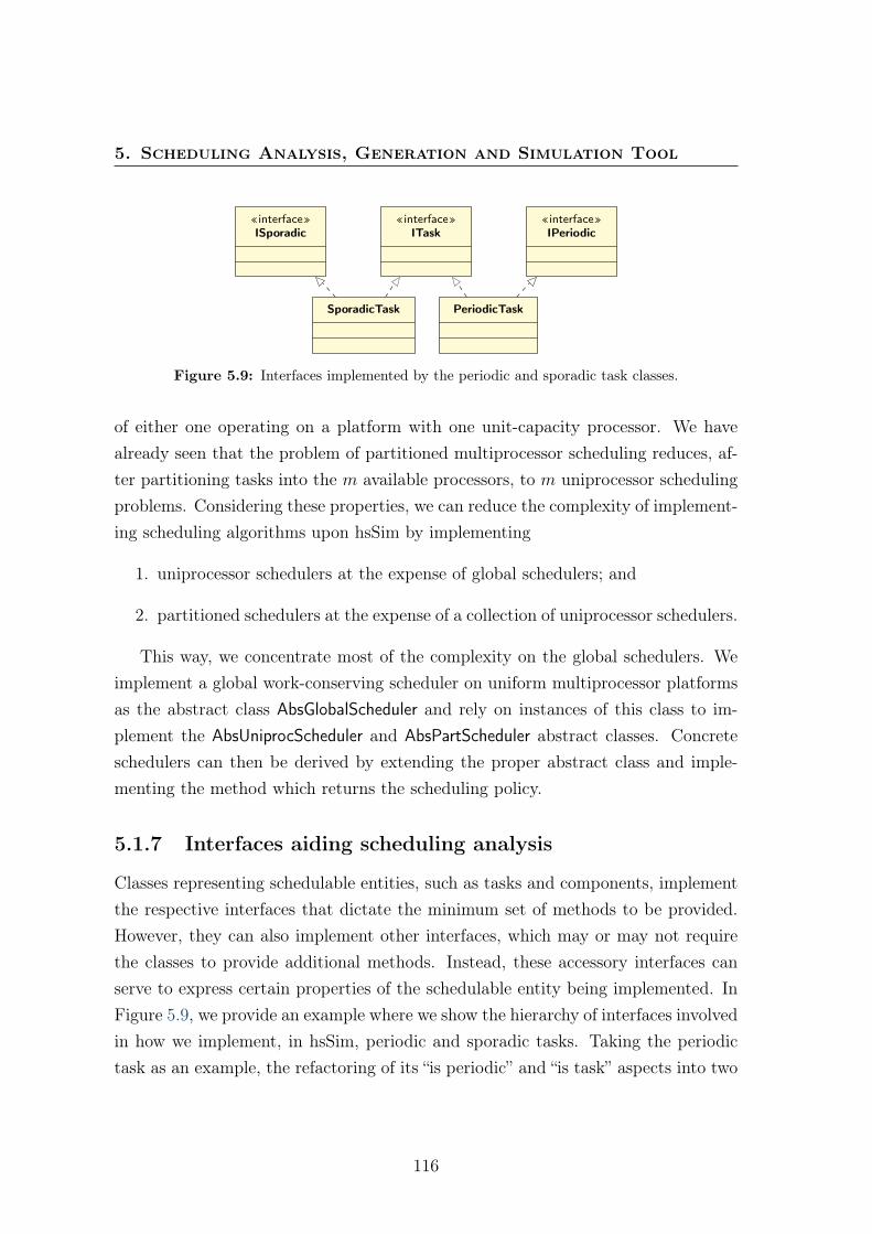
5. Scheduling Analysis, Generation and Simulation Tool

SporadicTask PeriodicTask

«interface»ISporadic

«interface»IPeriodic

«interface»ITask

Figure 5.9: Interfaces implemented by the periodic and sporadic task classes.

of either one operating on a platform with one unit-capacity processor. We havealready seen that the problem of partitioned multiprocessor scheduling reduces, af-ter partitioning tasks into the m available processors, to m uniprocessor schedulingproblems. Considering these properties, we can reduce the complexity of implement-ing scheduling algorithms upon hsSim by implementing

1. uniprocessor schedulers at the expense of global schedulers; and

2. partitioned schedulers at the expense of a collection of uniprocessor schedulers.

This way, we concentrate most of the complexity on the global schedulers. Weimplement a global work-conserving scheduler on uniform multiprocessor platformsas the abstract class AbsGlobalScheduler and rely on instances of this class to im-plement the AbsUniprocScheduler and AbsPartScheduler abstract classes. Concreteschedulers can then be derived by extending the proper abstract class and imple-menting the method which returns the scheduling policy.

5.1.7 Interfaces aiding scheduling analysis

Classes representing schedulable entities, such as tasks and components, implementthe respective interfaces that dictate the minimum set of methods to be provided.However, they can also implement other interfaces, which may or may not requirethe classes to provide additional methods. Instead, these accessory interfaces canserve to express certain properties of the schedulable entity being implemented. InFigure 5.9, we provide an example where we show the hierarchy of interfaces involvedin how we implement, in hsSim, periodic and sporadic tasks. Taking the periodictask as an example, the refactoring of its “is periodic” and “is task” aspects into two

116

5.1 Object-oriented analysis and design

separate interfaces allows having tasks which are not periodic (e. g., sporadic tasks)and periodic entities which are not tasks (namely, periodic components).

The rationale for the introduction of these interfaces is the potential to aid theselection of the appropriate scheduling analysis methdology— for instance, verifyingif a task set being verified for schedulability complies with the system model theschedulability test assumes (Gaudel et al., 2013). With these interfaces, coupledwith the multiprocessor scheduler taxonomy that we described in Section 5.1.6,these aids can be implemented resorting to Java’s instanceof primitive, applied tothe schedulable entities (e. g., tasks) and to the scheduler(s) of the target system.We have implemented so far only compositional analysis techniques, so the potentialof this approach is not yet fully noticeable.

5.1.8 Compositional analysis with the Decorator pattern

The Decorator pattern (Gamma et al., 1997) allows adding responsibilities to objectsof a given class without extending it. There are many valid reasons to avoid relyingon inheritance, especially when there is no full access to the class being augmented.Without full knowledge of the implementation of the latter, we may be unknowinglyoverriding methods which are used by other methods (thus modifying their behav-ior). It may also be the case that we want to add responsibilities to a class whichcannot be extended (final modifier, in Java). Finally, adding responsibilities throughdecoration instead of inheritance also allows circumventing the absence of multipleinheritance in most object-oriented programming languages.

We employ the Decorator pattern to add compositional analysis aspects to thenotion of component, as pictured in Figure 5.10. The CompositionalComponent classimplements the IComponent interface, and decorates an instance of a class thatalso implements the IComponent interface (in our case, the BasicComponent class).Instances of the CompositionalComponent class are not instances of the BasicCom-

ponent class, but rather hold a reference to an instance of the BasicComponent classto preserve and reuse the latter’s behavior when possible.

The additional responsibilities added by the CompositionalComponent class arethose required by the ICompositional interface, which depend on the use of a resourcemodel. The UMPR class implements the IResourceModel interface, and each instance

117

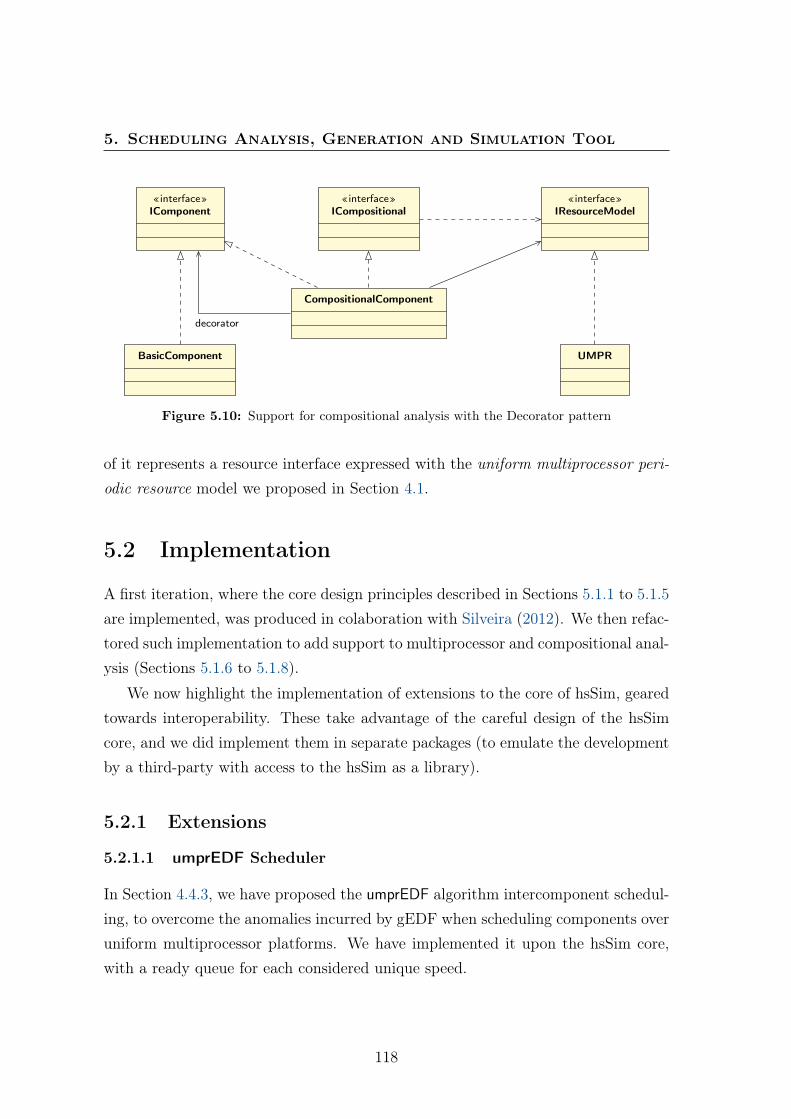
5. Scheduling Analysis, Generation and Simulation Tool

decorator

«interface»IComponent

«interface»ICompositional

«interface»IResourceModel

BasicComponent

CompositionalComponent

UMPR

Figure 5.10: Support for compositional analysis with the Decorator pattern

of it represents a resource interface expressed with the uniform multiprocessor peri-odic resource model we proposed in Section 4.1.

5.2 Implementation

A first iteration, where the core design principles described in Sections 5.1.1 to 5.1.5are implemented, was produced in colaboration with Silveira (2012). We then refac-tored such implementation to add support to multiprocessor and compositional anal-ysis (Sections 5.1.6 to 5.1.8).

We now highlight the implementation of extensions to the core of hsSim, gearedtowards interoperability. These take advantage of the careful design of the hsSimcore, and we did implement them in separate packages (to emulate the developmentby a third-party with access to the hsSim as a library).

5.2.1 Extensions

5.2.1.1 umprEDF Scheduler

In Section 4.4.3, we have proposed the umprEDF algorithm intercomponent schedul-ing, to overcome the anomalies incurred by gEDF when scheduling components overuniform multiprocessor platforms. We have implemented it upon the hsSim core,with a ready queue for each considered unique speed.

118

5.2 Implementation

Table 5.1: Mapping between hsSim events and Grasp trace content.

Event hsSim class Grasp log

Job arrives JobReleasedEventIf job of a task: jobArrivedIf job of a component: serverReplenished

Job obtains processor JobPreemptionEventaIf job of a task: jobResumedIf job of a component: serverResumed

Job preempted by another JobPreemptionEventIf job of a task: jobPreemptedb

If job of a component: serverPreemptedb

Job completes execution JobCompletedEventIf job of a task: jobCompletedIf job of a component: serverDepleted

a With a null preempted event.b Plus the appropriate jobResumed/serverResumed event.

5.2.1.2 Grasp logger

Because of our low coupling design for the event logging, it is straightforward to tracethe simulation to the format interpreted by Grasp Player (Holenderski et al., 2013).When we started this work, Grasp Player did not support uniform multiprocessors,namely with respect to tracing the component’s budget consumption according torates different from one unit of budget per unit of time; we have implemented thisfunctionality on Grasp Player.2

As said, the Grasp logger is implemented exactly as if it were developed by anexternal team, who could even only have access to the hsSim core as a library. Weimplement the Logger generic interface, instantiating its type variable with the Stringtype, since we want the processing (visit) of events to return the text to be addedto the Grasp trace. The visit methods are invoked when an event notification isreceived, via the update method. Invocation is done indirectly through the accept

method, so the right visit method is automatically selected and called.

Along the visit methods, we implement the mapping between hsSim events andGrasp trace content shown in Table 5.1. Listing 5.1 shows an example excerpt of atrace generated by hsSim’s Grasp Logger.

2We provided our patch to the developers of Grasp, and it was merged in version 1.8.

119

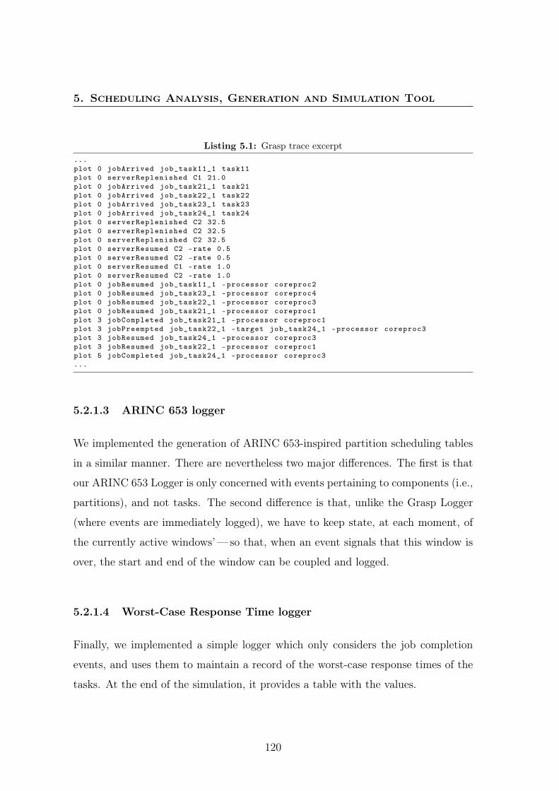
5. Scheduling Analysis, Generation and Simulation Tool

Listing 5.1: Grasp trace excerpt...plot 0 jobArrived job_task11_1 task11plot 0 serverReplenished C1 21.0plot 0 jobArrived job_task21_1 task21plot 0 jobArrived job_task22_1 task22plot 0 jobArrived job_task23_1 task23plot 0 jobArrived job_task24_1 task24plot 0 serverReplenished C2 32.5plot 0 serverReplenished C2 32.5plot 0 serverReplenished C2 32.5plot 0 serverResumed C2 -rate 0.5plot 0 serverResumed C2 -rate 0.5plot 0 serverResumed C1 -rate 1.0plot 0 serverResumed C2 -rate 1.0plot 0 jobResumed job_task11_1 -processor coreproc2plot 0 jobResumed job_task23_1 -processor coreproc4plot 0 jobResumed job_task22_1 -processor coreproc3plot 0 jobResumed job_task21_1 -processor coreproc1plot 3 jobCompleted job_task21_1 -processor coreproc1plot 3 jobPreempted job_task22_1 -target job_task24_1 -processor coreproc3plot 3 jobResumed job_task24_1 -processor coreproc3plot 3 jobResumed job_task22_1 -processor coreproc1plot 5 jobCompleted job_task24_1 -processor coreproc3...

5.2.1.3 ARINC 653 logger

We implemented the generation of ARINC 653-inspired partition scheduling tables

in a similar manner. There are nevertheless two major differences. The first is that

our ARINC 653 Logger is only concerned with events pertaining to components (i.e.,

partitions), and not tasks. The second difference is that, unlike the Grasp Logger

(where events are immediately logged), we have to keep state, at each moment, of

the currently active windows’— so that, when an event signals that this window is

over, the start and end of the window can be coupled and logged.

5.2.1.4 Worst-Case Response Time logger

Finally, we implemented a simple logger which only considers the job completion

events, and uses them to maintain a record of the worst-case response times of the

tasks. At the end of the simulation, it provides a table with the values.

120

5.3 Example use case

5.3 Example use case

We now use an example use case to provide a deeper explanation of the schedulinganalysis, simulation and schedule generation functionalities that we have imple-mented. This example also serves the purpose of demonstrating the formal methodsproposed and results described in Chapter 4. For this reason, let us consider thesame example that we saw in Section 4.4.4: two components, C1 and C2, containinggEDF-scheduled sporadic task sets

T1 = {(21, 19, 21)} and T2 = {(20, 3, 20), (20, 4, 20), (20, 4, 20), (20, 1, 20)} ,

respectively.

5.3.1 Scheduling analysis

With the period and virtual platform for each component’s resource interface be-ing provided by the system designer, hsSim calculates (in the case of the UMPRmodel) the minimum value for Θ that guarantees schedulability of the enclosedtask set. As before, we will use the least minimum interarrival time among eachtask set as the period for the respective component. With those values, we obtainthe same resource interfaces as we saw in Section 4.4.4: U1 = (21, 21, {1.0}) andU2 = (20, 32.5, {1.0, 0.5, 0.5}). hsSim automatically generates the correspondinginterface tasks, which will then be used to release jobs of the component.

5.3.2 Scheduling simulation and visualization

We have simulated the execution of the system comprising components C1 and C2

with both gEDF and umprEDF intercomponent scheduling algorithms. The resultsof the simulation are provided by the considered loggers. In our case, we employedloggers to register worst-case response times, to create a trace to be visualized withGrasp, and to generate an ARINC 653-like partition scheduling table. We nowanalyze the information provided by the worst-case response time and Grasp loggers;we analyze the partition scheduling table generation in the next section.

121

5. Scheduling Analysis, Generation and Simulation Tool

Sporadic tasks release their jobs with a minimum separation, whereas periodictasks release their jobs with a constant separation. For this reason, to have resultscloser to the reality of sporadic tasks, we have introduced a fixed release jitter. Wehave performed simulations with jitters between 0 and 12. The semantics of thisfixed jitter (let us denote it as j) is that every job of a task τp,i is released Tp,i + j′

time units after the previous job of the same task, where j′ is a random integernumber in the interval [0, j]. The values of j′ are generated by per-task randomnumber generators, which are initialized with a task-specific seed when the task iscreated; this is to allow the job releases to happen at the same time instants whensimulating with each of the intercomponent scheduling algorithms (as thus allow theresults to be comparable).

In Figure 5.11, we can see the worst-case response times of the five tasks in thesystem; we highlight task τ1,1, since the remaining tasks have the same worst-caseresponse time with gEDF and with umprEDF. The dashed horizontal line in eachgraph represents the respective task’s relative deadline. We see that, when usinggEDF for intercomponent scheduling, task τ1,1 yielded a worst-case response timelonger than its relative deadline, which means that one or more of its jobs missedtheir deadlines.

What we see here is the consequence of the phenomenon we predicted analyticallyin Section 4.4.2. Although the components are abstracted with resource interfacesderived to guarantee schedulability, gEDF does not guarantee that the componentshave the resource supply therein expressed (namely in terms of virtual platform).We can verify this by visualizing, in Grasp, the trace recorded for this simulation,shown in Figure 5.12). The execution of the task in component C1 is traced in darkgray bars, whereas that of tasks in component C2 is traced in light gray bars. Atthe bottom of the figure, we have traced the remaining budget of each component,which corresponds to the total remaining execution time of the interface tasks ofits resource interface. We can see, right at time instant 0, that the tasks in C2 takeover the three fastest processors, including two 1.0-speed processors, although thevirtual platform considered for it had only one 1.0-speed processor. Component C1

is relegated to the fourth processor, with speed s0,4 = 0.5, although the resourceinterface U1 only considered one processor of speed 1.0. This anomaly has an effecton the resource provision given to component C1. As can be seen in the budget traces

122

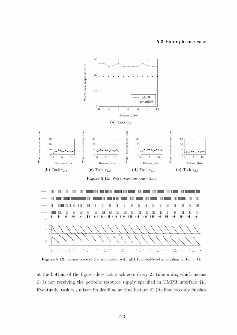
5.3 Example use case

0 2 4 6 8 10 120

10

20

30

Release jitter

Worst-caserespon

setime

gEDFumprEDF

(a) Task τ1,1

0 5 100

10

20

30

Release jitterWor

st-c

ase

resp

onse

tim

e

(b) Task τ2,1

0 5 100

10

20

30

Release jitterWor

st-c

ase

resp

onse

tim

e

(c) Task τ2,2

0 5 100

10

20

30

Release jitterWor

st-c

ase

resp

onse

tim

e

(d) Task τ2,3

0 5 100

10

20

30

Release jitterWor

st-c

ase

resp

onse

tim

e(e) Task τ2,4

Figure 5.11: Worst-case response time

0 50 100 150 200 250 300 350 400

0

11

21

0

16

33

coreproc1

coreproc2

coreproc3

coreproc4

main

C1

C2

Figure 5.12: Grasp trace of the simulation with gEDF global-level scheduling (jitter = 1).

at the bottom of the figure, does not reach zero every 21 time units, which means

C1 is not receiving the periodic resource supply specified in UMPR interface U1.

Eventually, task τ1,1 misses its deadline at time instant 21 (its first job only finishes

123

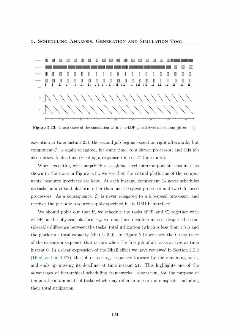
5. Scheduling Analysis, Generation and Simulation Tool

0 50 100 150 200 250 300 350 400

0

11

21

0

16

33

coreproc1

coreproc2

coreproc3

coreproc4

main

C1

C2

Figure 5.13: Grasp trace of the simulation with umprEDF global-level scheduling (jitter = 1).

execution at time instant 25); the second job begins execution right afterwards, but

component C1 is again relegated, for some time, to a slower processor, and this job

also misses its deadline (yielding a response time of 27 time units).

When executing with umprEDF as a global-level intercomponent scheduler, as

shown in the trace in Figure 5.13, we see that the virtual platforms of the compo-

nents’ resource interfaces are kept. At each instant, component C2 never schedules

its tasks on a virtual platform other than one 1.0-speed processor and two 0.5-speed

processors. As a consequence, C1 is never relegated to a 0.5-speed processor, and

receives the periodic resource supply specified in its UMPR interface.

We should point out that if, we schedule the tasks of T1 and T2 together with

gEDF on the physical platform π0, we may have deadline misses, despite the con-

siderable difference between the tasks’ total utilization (which is less than 1.51) and

the platform’s total capacity (that is 3.0). In Figure 5.14 we show the Grasp trace

of the execution sequence that occurs when the first job of all tasks arrives at time

instant 0. In a clear expression of the Dhall effect we have reviewed in Section 2.2.2

(Dhall & Liu, 1978), the job of task τ1,1 is pushed forward by the remaining tasks,

and ends up missing its deadline at time instant 21. This highlights one of the

advantages of hierarchical scheduling frameworks: separation, for the purpose of

temporal containment, of tasks which may differ in one or more aspects, including

their total utilization.

124

5.4 Summary

0 5 10 15 20

coreproc1

coreproc2

coreproc3

coreproc4

main

Figure 5.14: Grasp trace for the simulation of task set T1∪T2 being scheduled with gEDF directlyon the physical platform.

5.3.3 Schedule generation

The type of XML file generated by hsSim is illustrated in Listing 5.2. As in the for-mat prescribed by the ARINC 653 specification, the Module_Schedule node containsthe partition scheduling table itself, whereas as the remaining nodes contain config-uration information; in our case, the latter includes a new node, Module_Platform,pertaining to the processors.

In the ARINC 653 format, the Module_Schedule node contains the partitionscheduling table divided in Partition_Schedule sub-nodes. We retain this structure,since it is convenient for verification purpose; the set of scheduling windows can beanalyzed to assess if it adds up to the partition’s periodic requirement (expressedin the PeriodExecutionRequirement and Period attributes). We do however add analternative representation of the partition scheduling table, tailored at the onlinescheduling process itself. For the generation of this representation, periods where aprocessor was not (in the logged simulation) assigned to any partition are assignedto the last partition to which the processor was assigned. This allows simplifying thescheduling decisions taken in execution time and drastically reducing the number ofpartition preemptions.

5.4 Summary

In this chapter, we have described the design, development and use of hsSim, ascheduling analysis, generation and simulation tool with a focus on hierachicalscheduling, extensibility and interoperability. The two latter aspects were dealt

125

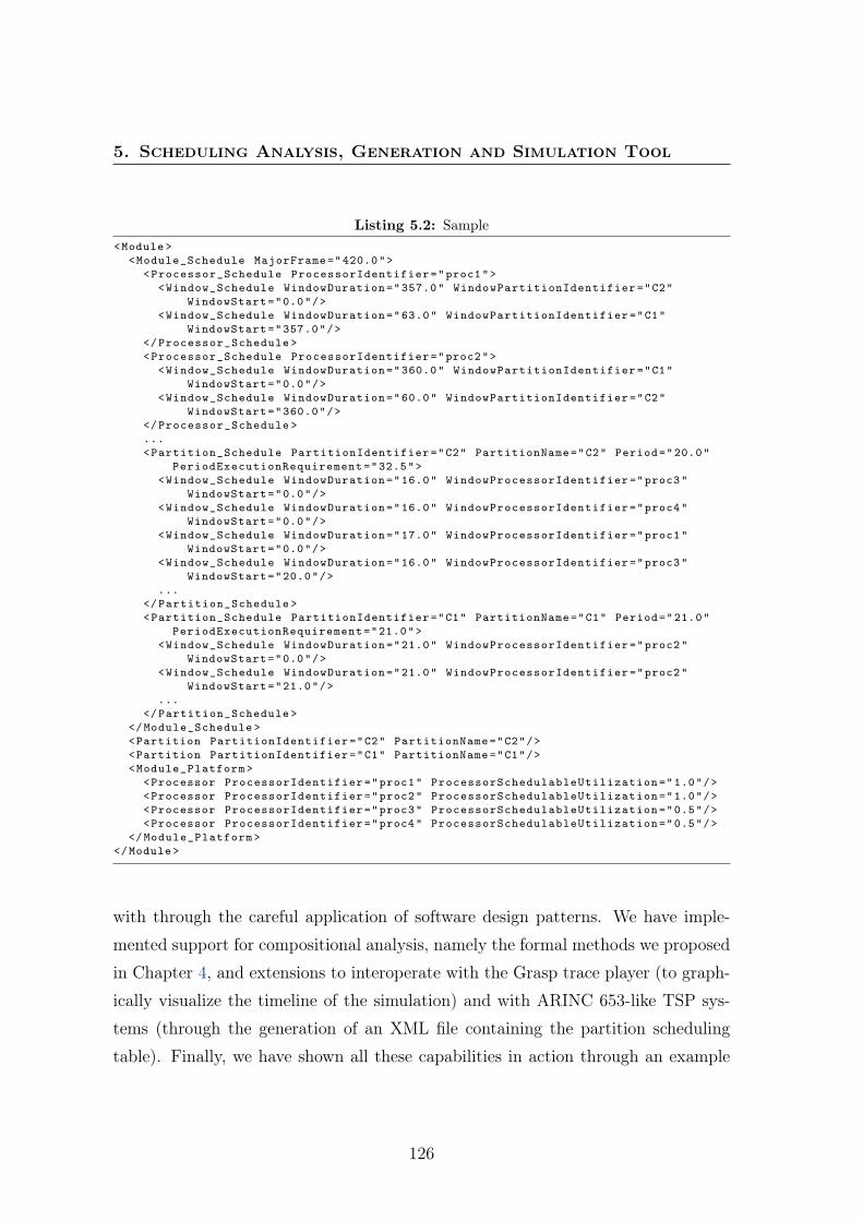
5. Scheduling Analysis, Generation and Simulation Tool

Listing 5.2: Sample<Module >

<Module_Schedule MajorFrame="420.0"><Processor_Schedule ProcessorIdentifier="proc1">

<Window_Schedule WindowDuration="357.0" WindowPartitionIdentifier="C2"WindowStart="0.0"/>

<Window_Schedule WindowDuration="63.0" WindowPartitionIdentifier="C1"WindowStart="357.0"/>

</Processor_Schedule ><Processor_Schedule ProcessorIdentifier="proc2">

<Window_Schedule WindowDuration="360.0" WindowPartitionIdentifier="C1"WindowStart="0.0"/>

<Window_Schedule WindowDuration="60.0" WindowPartitionIdentifier="C2"WindowStart="360.0"/>

</Processor_Schedule >...<Partition_Schedule PartitionIdentifier="C2" PartitionName="C2" Period="20.0"

PeriodExecutionRequirement="32.5"><Window_Schedule WindowDuration="16.0" WindowProcessorIdentifier="proc3"

WindowStart="0.0"/><Window_Schedule WindowDuration="16.0" WindowProcessorIdentifier="proc4"

WindowStart="0.0"/><Window_Schedule WindowDuration="17.0" WindowProcessorIdentifier="proc1"

WindowStart="0.0"/><Window_Schedule WindowDuration="16.0" WindowProcessorIdentifier="proc3"

WindowStart="20.0"/>...

</Partition_Schedule ><Partition_Schedule PartitionIdentifier="C1" PartitionName="C1" Period="21.0"

PeriodExecutionRequirement="21.0"><Window_Schedule WindowDuration="21.0" WindowProcessorIdentifier="proc2"

WindowStart="0.0"/><Window_Schedule WindowDuration="21.0" WindowProcessorIdentifier="proc2"

WindowStart="21.0"/>...

</Partition_Schedule ></Module_Schedule ><Partition PartitionIdentifier="C2" PartitionName="C2"/><Partition PartitionIdentifier="C1" PartitionName="C1"/><Module_Platform >

<Processor ProcessorIdentifier="proc1" ProcessorSchedulableUtilization="1.0"/><Processor ProcessorIdentifier="proc2" ProcessorSchedulableUtilization="1.0"/><Processor ProcessorIdentifier="proc3" ProcessorSchedulableUtilization="0.5"/><Processor ProcessorIdentifier="proc4" ProcessorSchedulableUtilization="0.5"/>

</Module_Platform ></Module >

with through the careful application of software design patterns. We have imple-

mented support for compositional analysis, namely the formal methods we proposed

in Chapter 4, and extensions to interoperate with the Grasp trace player (to graph-

ically visualize the timeline of the simulation) and with ARINC 653-like TSP sys-

tems (through the generation of an XML file containing the partition scheduling

table). Finally, we have shown all these capabilities in action through an example

126

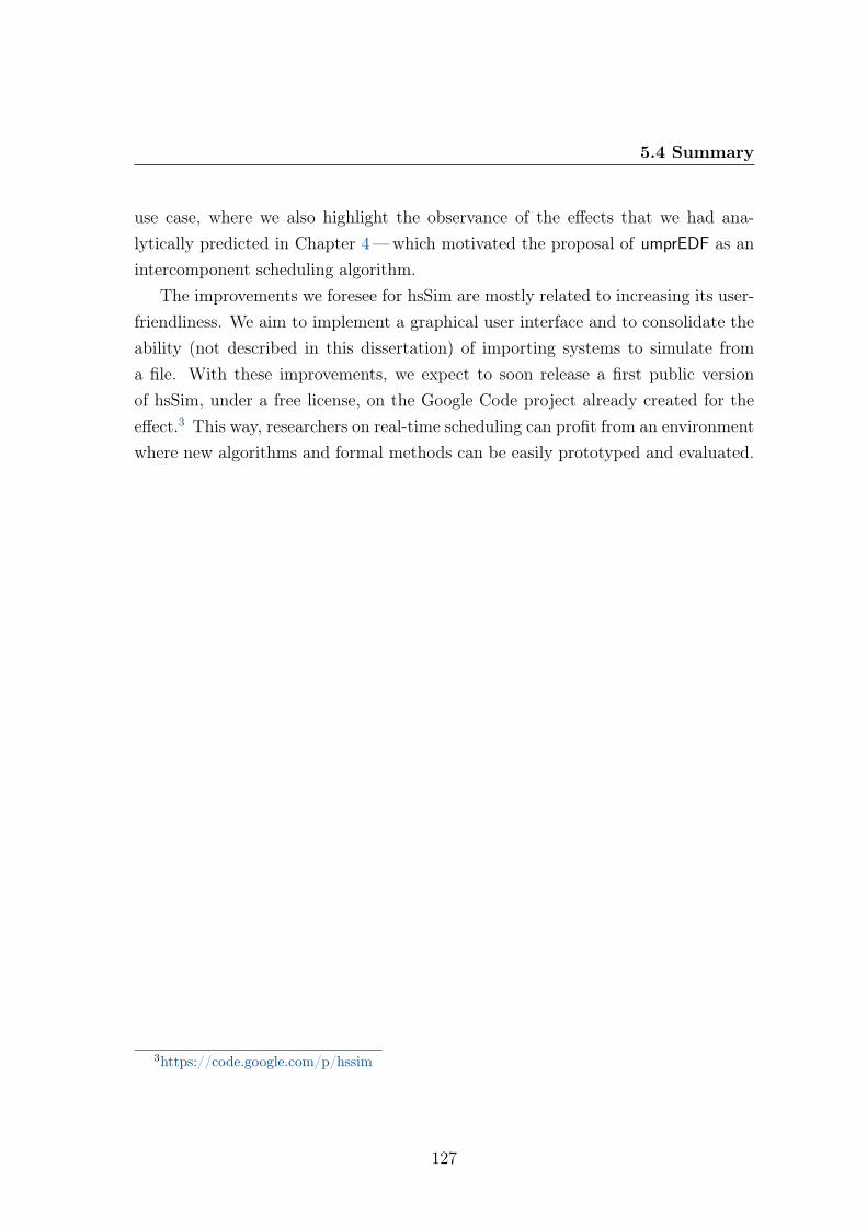
5.4 Summary

use case, where we also highlight the observance of the effects that we had ana-lytically predicted in Chapter 4—which motivated the proposal of umprEDF as anintercomponent scheduling algorithm.

The improvements we foresee for hsSim are mostly related to increasing its user-friendliness. We aim to implement a graphical user interface and to consolidate theability (not described in this dissertation) of importing systems to simulate froma file. With these improvements, we expect to soon release a first public versionof hsSim, under a free license, on the Google Code project already created for theeffect.3 This way, researchers on real-time scheduling can profit from an environmentwhere new algorithms and formal methods can be easily prototyped and evaluated.

3https://code.google.com/p/hssim

127

Chapter 6

Towards Self-Adaptation in Time-and Space-Partitioned Systems

In this chapter, we present preliminary results on self-adaptation in TSP systems.These results serve the purpose of sustaining our statement that the active ex-ploitation of employing multiple processor cores can open room for supporting self-adaptive behavior to cope with unforeseen changes in operational and environmentalconditions (Section 1.3).

We begin, in Section 6.1, by describing with more detail the monitoring and adap-tation mechanisms in the AIR architecture (which we presented in Section 3.1.2).1

We also perform an evaluation of these mechanisms on a prototype implementationof an AIR system. Then we propose how to take advantage of these mechanisms toachieve self-adaptive behavior in TSP systems, and evaluate our proposal throughsimulation experiments (Section 6.2). In Section 6.3, we discuss extensions whichcan improve the coverage of the described self-adaptation approach, based on mul-tiprocessor platforms, reconfiguration, and proactive fault tolerance.

6.1 Monitoring and adaptation mechanisms

We now describe AIR’s monitoring (deadline violation detection) and adaptation(mode-based schedules) mechanisms, and their relation to ARINC 653-related as-

1These mechanisms were first introduced in the scope of the author’s Master thesis (Craveiro,2009) and consolidated in the scope of the hereby described work.

129

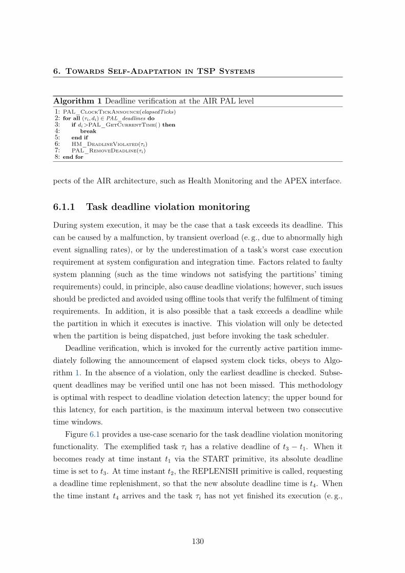
6. Towards Self-Adaptation in TSP Systems

Algorithm 1 Deadline verification at the AIR PAL level1: PAL_ClockTickAnnounce(elapsedTicks)2: for all (τi, di) ∈ PAL_deadlines do3: if di>PAL_GetCurrentTime( ) then4: break5: end if6: HM_DeadlineViolated(τi)7: PAL_RemoveDeadline(τi)8: end for

pects of the AIR architecture, such as Health Monitoring and the APEX interface.

6.1.1 Task deadline violation monitoring

During system execution, it may be the case that a task exceeds its deadline. Thiscan be caused by a malfunction, by transient overload (e. g., due to abnormally highevent signalling rates), or by the underestimation of a task’s worst case executionrequirement at system configuration and integration time. Factors related to faultysystem planning (such as the time windows not satisfying the partitions’ timingrequirements) could, in principle, also cause deadline violations; however, such issuesshould be predicted and avoided using offline tools that verify the fulfilment of timingrequirements. In addition, it is also possible that a task exceeds a deadline whilethe partition in which it executes is inactive. This violation will only be detectedwhen the partition is being dispatched, just before invoking the task scheduler.

Deadline verification, which is invoked for the currently active partition imme-diately following the announcement of elapsed system clock ticks, obeys to Algo-rithm 1. In the absence of a violation, only the earliest deadline is checked. Subse-quent deadlines may be verified until one has not been missed. This methodologyis optimal with respect to deadline violation detection latency; the upper bound forthis latency, for each partition, is the maximum interval between two consecutivetime windows.

Figure 6.1 provides a use-case scenario for the task deadline violation monitoringfunctionality. The exemplified task τi has a relative deadline of t3 − t1. When itbecomes ready at time instant t1 via the START primitive, its absolute deadlinetime is set to t3. At time instant t2, the REPLENISH primitive is called, requestinga deadline time replenishment, so that the new absolute deadline time is t4. Whenthe time instant t4 arrives and the task τi has not yet finished its execution (e. g.,

130

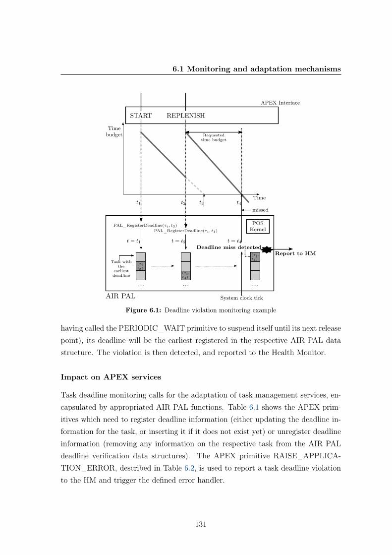
6.1 Monitoring and adaptation mechanisms

APEX Interface

POSKernel

START REPLENISH

t1 t2 t3 t4

AIR PAL

Deadline miss detected

PAL_RegisterDeadline(τi, t3)

PAL_RegisterDeadline(τi, t1)

t = t1 t = t2 t = t4

... ... ...

Task withthe

earliestdeadline

System clock tick

missed

Time

Requestedtime budget

Report to HM

(τi,t3)

(τi,t4)

(τi,t4)

Timebudget

Figure 6.1: Deadline violation monitoring example

having called the PERIODIC_WAIT primitive to suspend itself until its next releasepoint), its deadline will be the earliest registered in the respective AIR PAL datastructure. The violation is then detected, and reported to the Health Monitor.

Impact on APEX services

Task deadline monitoring calls for the adaptation of task management services, en-capsulated by appropriated AIR PAL functions. Table 6.1 shows the APEX prim-itives which need to register deadline information (either updating the deadline in-formation for the task, or inserting it if it does not exist yet) or unregister deadlineinformation (removing any information on the respective task from the AIR PALdeadline verification data structures). The APEX primitive RAISE_APPLICA-TION_ERROR, described in Table 6.2, is used to report a task deadline violationto the HM and trigger the defined error handler.

131

6. Towards Self-Adaptation in TSP Systems

Table 6.1: APEX services in need of modifications to support task deadline violation monitoring

Primitive Short description

Need to register/update deadline[DELAYED_]START Start a task [with a given delay]PERIODIC_WAIT Suspend execution of a (periodic) task until the next release

pointREPLENISH Postpone a task’s deadline time

Need to unregister deadlineSTOP[_SELF] Stop a task [itself]

Table 6.2: Essential APEX services for Health Monitoring

Primitive Short description

RAISE_APPLICATION_ERROR Notify the error handler for a specific error type

Our task deadline violation monitoring mechanisms does not need particular al-gorithmic modifications to be used in multiprocessor settings, since there will beonly one AIR PAL instance per partition (regardless of the number of processorsto which the partition can have access). However, because of the potential for con-current modifications through the APEX interface (Table 6.1), the data structuresin the AIR PAL should be protected using appropriate synchronization mechanisms(e.g., readers–writer lock).

Relation to Health Monitor and error handling

In the context of fault detection and isolation, ARINC 653 classifies deadline viola-tion as a “process level error” —an error that impacts one or more processes (tasks)in the partition, or the entire partition (AEEC, 1997). The action to be performedin the event of an error is defined by the application programmer through an appro-priate error handler.

The error handler may an application task tailored for partition-wide error pro-cessing. In the case of spacecraft, the occurrence of task-/partition-level errors maybe signalled through interpartition communication to a (system partition) process

132

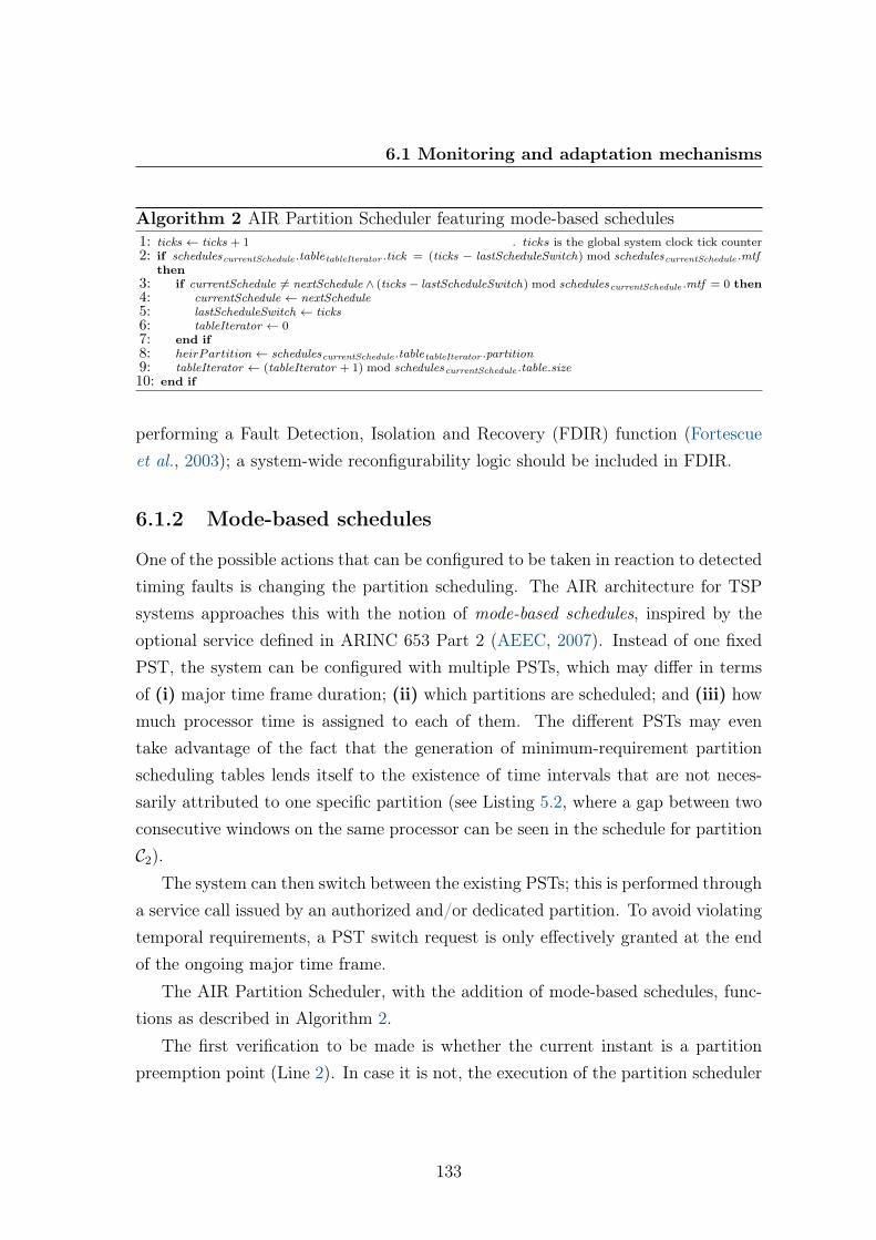
6.1 Monitoring and adaptation mechanisms

Algorithm 2 AIR Partition Scheduler featuring mode-based schedules1: ticks ← ticks + 1 . ticks is the global system clock tick counter2: if schedulescurrentSchedule .tabletableIterator .tick = (ticks − lastScheduleSwitch) mod schedulescurrentSchedule .mtf

then3: if currentSchedule 6= nextSchedule ∧ (ticks − lastScheduleSwitch) mod schedulescurrentSchedule .mtf = 0 then4: currentSchedule ← nextSchedule5: lastScheduleSwitch ← ticks6: tableIterator ← 07: end if8: heirPartition← schedulescurrentSchedule .tabletableIterator .partition9: tableIterator ← (tableIterator + 1) mod schedulescurrentSchedule .table.size10: end if

performing a Fault Detection, Isolation and Recovery (FDIR) function (Fortescueet al., 2003); a system-wide reconfigurability logic should be included in FDIR.

6.1.2 Mode-based schedules

One of the possible actions that can be configured to be taken in reaction to detectedtiming faults is changing the partition scheduling. The AIR architecture for TSPsystems approaches this with the notion of mode-based schedules, inspired by theoptional service defined in ARINC 653 Part 2 (AEEC, 2007). Instead of one fixedPST, the system can be configured with multiple PSTs, which may differ in termsof (i) major time frame duration; (ii) which partitions are scheduled; and (iii) howmuch processor time is assigned to each of them. The different PSTs may eventake advantage of the fact that the generation of minimum-requirement partitionscheduling tables lends itself to the existence of time intervals that are not neces-sarily attributed to one specific partition (see Listing 5.2, where a gap between twoconsecutive windows on the same processor can be seen in the schedule for partitionC2).

The system can then switch between the existing PSTs; this is performed througha service call issued by an authorized and/or dedicated partition. To avoid violatingtemporal requirements, a PST switch request is only effectively granted at the endof the ongoing major time frame.

The AIR Partition Scheduler, with the addition of mode-based schedules, func-tions as described in Algorithm 2.

The first verification to be made is whether the current instant is a partitionpreemption point (Line 2). In case it is not, the execution of the partition scheduler

133

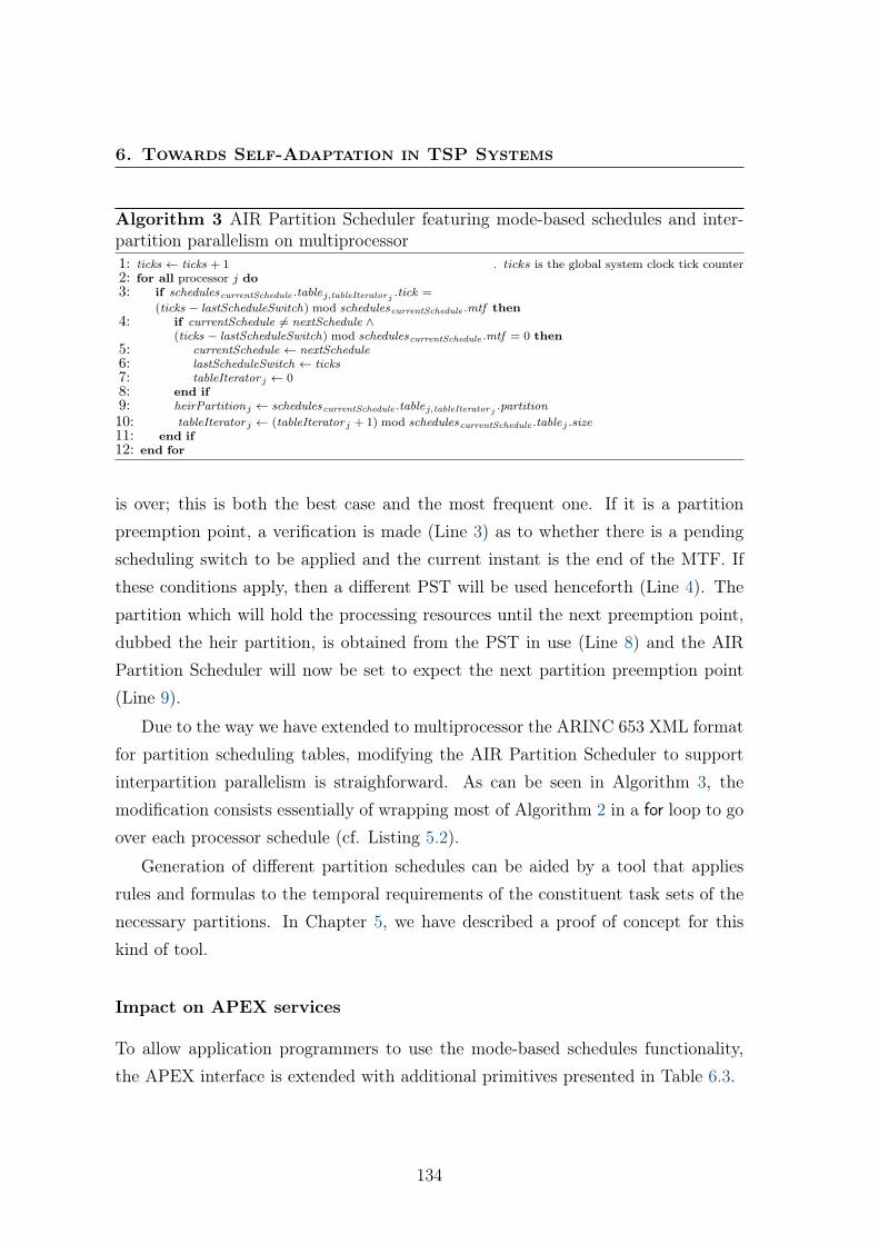
6. Towards Self-Adaptation in TSP Systems

Algorithm 3 AIR Partition Scheduler featuring mode-based schedules and inter-partition parallelism on multiprocessor1: ticks ← ticks + 1 . ticks is the global system clock tick counter2: for all processor j do3: if schedulescurrentSchedule .tablej,tableIteratorj .tick =

(ticks − lastScheduleSwitch) mod schedulescurrentSchedule .mtf then4: if currentSchedule 6= nextSchedule ∧

(ticks − lastScheduleSwitch) mod schedulescurrentSchedule .mtf = 0 then5: currentSchedule ← nextSchedule6: lastScheduleSwitch ← ticks7: tableIteratorj ← 08: end if9: heirPartitionj ← schedulescurrentSchedule .tablej,tableIteratorj .partition

10: tableIteratorj ← (tableIteratorj + 1) mod schedulescurrentSchedule .tablej .size11: end if12: end for

is over; this is both the best case and the most frequent one. If it is a partitionpreemption point, a verification is made (Line 3) as to whether there is a pendingscheduling switch to be applied and the current instant is the end of the MTF. Ifthese conditions apply, then a different PST will be used henceforth (Line 4). Thepartition which will hold the processing resources until the next preemption point,dubbed the heir partition, is obtained from the PST in use (Line 8) and the AIRPartition Scheduler will now be set to expect the next partition preemption point(Line 9).

Due to the way we have extended to multiprocessor the ARINC 653 XML formatfor partition scheduling tables, modifying the AIR Partition Scheduler to supportinterpartition parallelism is straighforward. As can be seen in Algorithm 3, themodification consists essentially of wrapping most of Algorithm 2 in a for loop to goover each processor schedule (cf. Listing 5.2).

Generation of different partition schedules can be aided by a tool that appliesrules and formulas to the temporal requirements of the constituent task sets of thenecessary partitions. In Chapter 5, we have described a proof of concept for thiskind of tool.

Impact on APEX services

To allow application programmers to use the mode-based schedules functionality,the APEX interface is extended with additional primitives presented in Table 6.3.

134

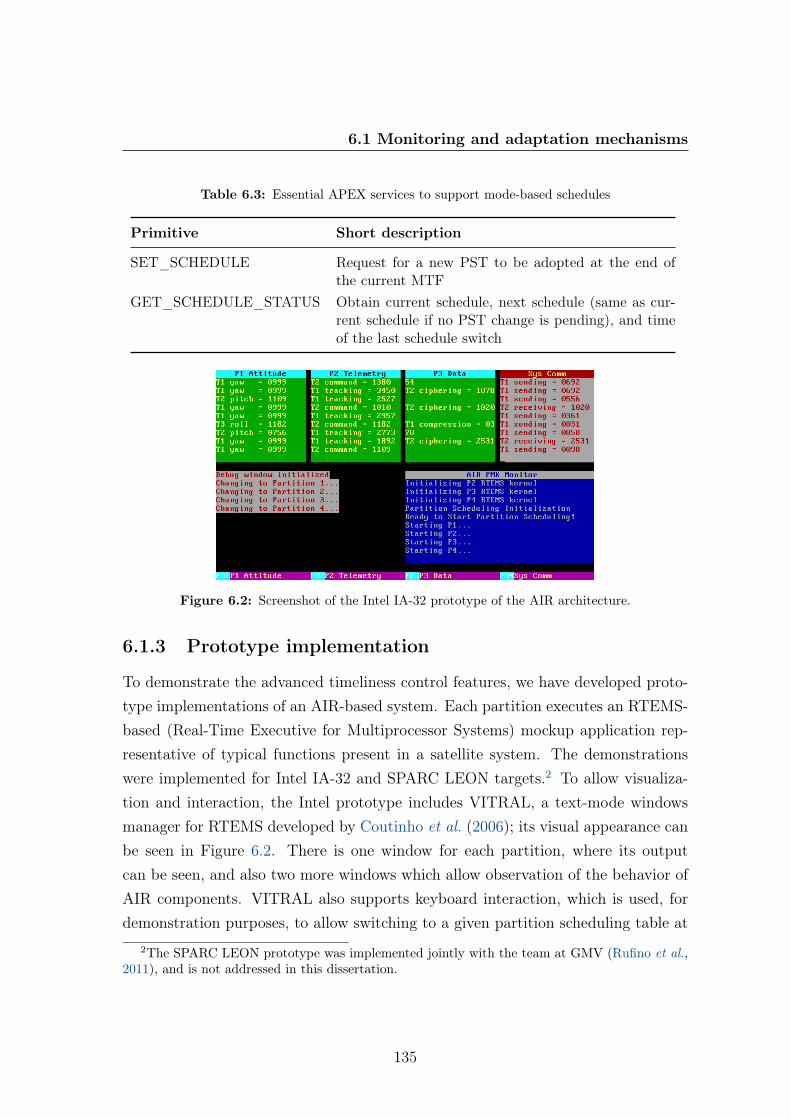
6.1 Monitoring and adaptation mechanisms

Table 6.3: Essential APEX services to support mode-based schedules

Primitive Short description

SET_SCHEDULE Request for a new PST to be adopted at the end ofthe current MTF

GET_SCHEDULE_STATUS Obtain current schedule, next schedule (same as cur-rent schedule if no PST change is pending), and timeof the last schedule switch

Figure 6.2: Screenshot of the Intel IA-32 prototype of the AIR architecture.

6.1.3 Prototype implementation

To demonstrate the advanced timeliness control features, we have developed proto-type implementations of an AIR-based system. Each partition executes an RTEMS-based (Real-Time Executive for Multiprocessor Systems) mockup application rep-resentative of typical functions present in a satellite system. The demonstrationswere implemented for Intel IA-32 and SPARC LEON targets.2 To allow visualiza-tion and interaction, the Intel prototype includes VITRAL, a text-mode windowsmanager for RTEMS developed by Coutinho et al. (2006); its visual appearance canbe seen in Figure 6.2. There is one window for each partition, where its outputcan be seen, and also two more windows which allow observation of the behavior ofAIR components. VITRAL also supports keyboard interaction, which is used, fordemonstration purposes, to allow switching to a given partition scheduling table at

2The SPARC LEON prototype was implemented jointly with the team at GMV (Rufino et al.,2011), and is not addressed in this dissertation.

135

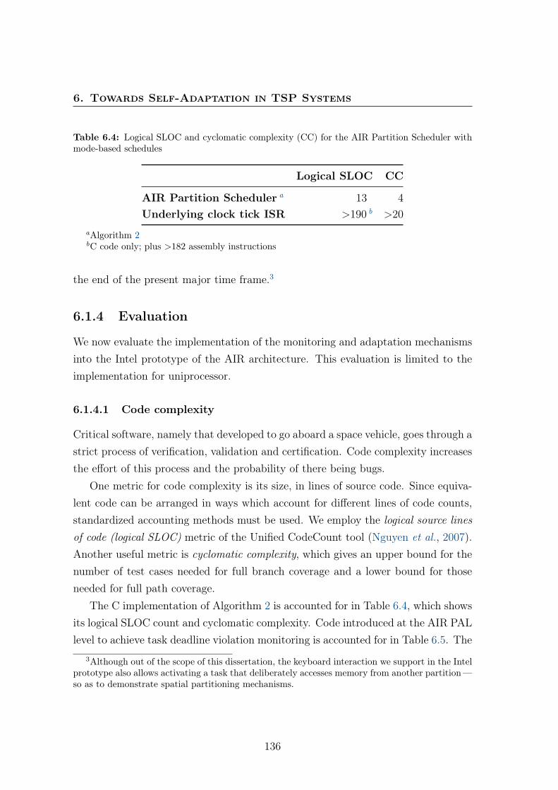
6. Towards Self-Adaptation in TSP Systems

Table 6.4: Logical SLOC and cyclomatic complexity (CC) for the AIR Partition Scheduler withmode-based schedules

Logical SLOC CC

AIR Partition Scheduler a 13 4Underlying clock tick ISR >190 b >20

aAlgorithm 2bC code only; plus >182 assembly instructions

the end of the present major time frame.3

6.1.4 Evaluation

We now evaluate the implementation of the monitoring and adaptation mechanismsinto the Intel prototype of the AIR architecture. This evaluation is limited to theimplementation for uniprocessor.

6.1.4.1 Code complexity

Critical software, namely that developed to go aboard a space vehicle, goes through astrict process of verification, validation and certification. Code complexity increasesthe effort of this process and the probability of there being bugs.

One metric for code complexity is its size, in lines of source code. Since equiva-lent code can be arranged in ways which account for different lines of code counts,standardized accounting methods must be used. We employ the logical source linesof code (logical SLOC) metric of the Unified CodeCount tool (Nguyen et al., 2007).Another useful metric is cyclomatic complexity, which gives an upper bound for thenumber of test cases needed for full branch coverage and a lower bound for thoseneeded for full path coverage.

The C implementation of Algorithm 2 is accounted for in Table 6.4, which showsits logical SLOC count and cyclomatic complexity. Code introduced at the AIR PALlevel to achieve task deadline violation monitoring is accounted for in Table 6.5. The

3Although out of the scope of this dissertation, the keyboard interaction we support in the Intelprototype also allows activating a task that deliberately accesses memory from another partition—so as to demonstrate spatial partitioning mechanisms.

136

6.1 Monitoring and adaptation mechanisms

Table 6.5: Logical SLOC and cyclomatic complexity (CC) for the implementation of deadlineviolation monitoring in AIR PAL

Logical SLOC CC

Register deadline 34 6Unregister deadline 12 3Verify deadlines a 16 2

aAlgorithm 1

total complexity added in terms of code executed during a clock tick ISR is a smallfraction of that already present in the underlying ISR code.

6.1.4.2 Computational complexity analysis

Since the verifications of deadlines and of the need to apply a new PST are exe-cuted inside the system clock tick ISR, they must have a bounded execution time;computational complexity is a good indicator thereof.

In the AIR Partition Scheduler (Algorithm 2), all instructions are O(1). Accessesto multielement structures are made by index, and thus their complexity does notdepend on the number of elements or the position of the desired element.

Linear complexity is easily achievable for the majority of the executions of thetask deadline verification at the AIR PAL level (Algorithm 1). By placing deadlinesin a linked list in ascending order of deadline times, the earliest deadline is retrievedin constant time. The removal of a violated deadline from the data structure canalso be made in constant time, since we already hold a pointer for the said deadline.In case of deadline violation, the next deadline(s) will successively be verified untilreaching one that has not expired. Thus, the worst case yields O(n), where n isthe number of tasks in the partition. However, by design, the number of tasksis bounded, and these worst cases are highly exceptional and mean the total andcomplete failure of the partition, which should be signalled to the HM.

6.1.4.3 Basic execution metrics

AIR Partition Scheduler execution time has been measured, resulting in the basicmetrics shown in Table 6.6. The second row shows the minimum, maximum and

137

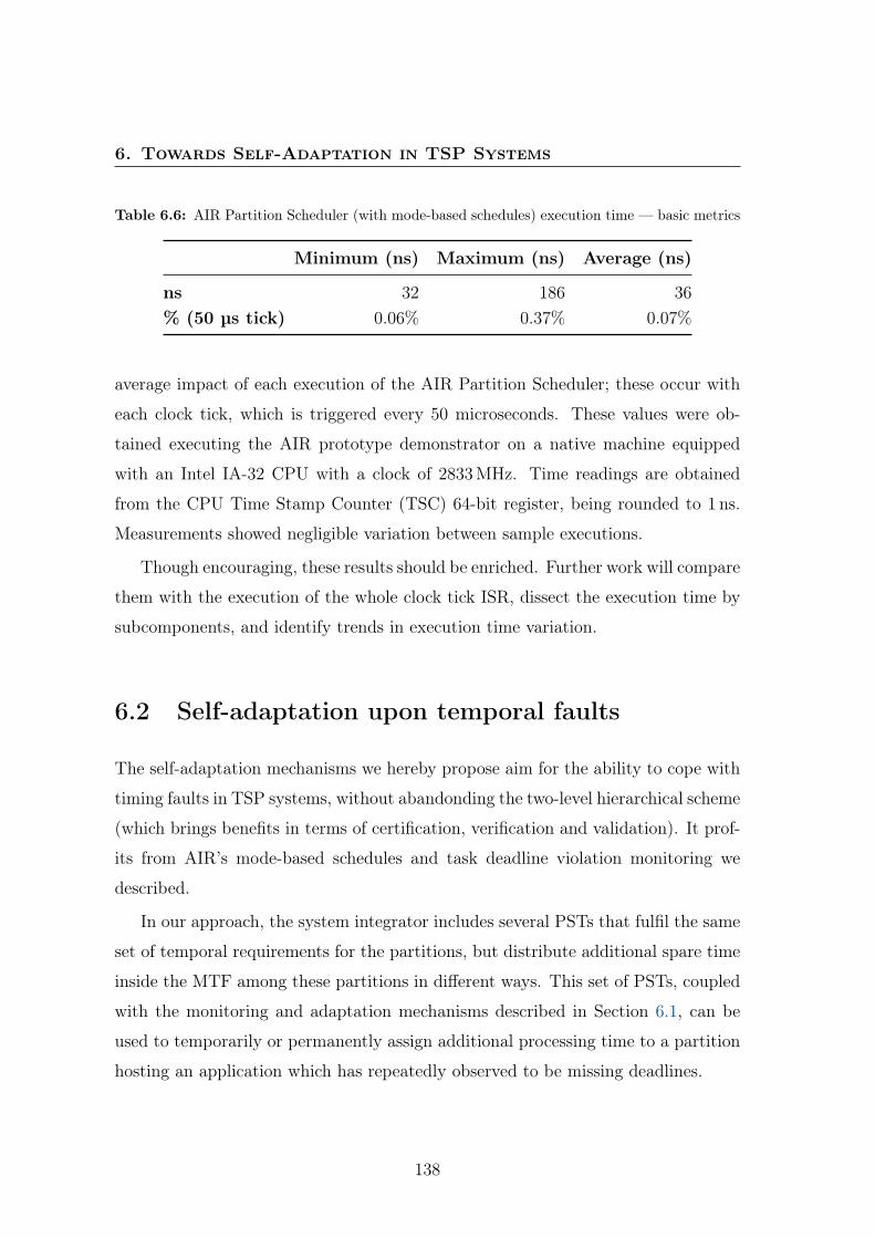
6. Towards Self-Adaptation in TSP Systems

Table 6.6: AIR Partition Scheduler (with mode-based schedules) execution time — basic metrics

Minimum (ns) Maximum (ns) Average (ns)

ns 32 186 36% (50 µs tick) 0.06% 0.37% 0.07%

average impact of each execution of the AIR Partition Scheduler; these occur with

each clock tick, which is triggered every 50 microseconds. These values were ob-

tained executing the AIR prototype demonstrator on a native machine equipped

with an Intel IA-32 CPU with a clock of 2833MHz. Time readings are obtained

from the CPU Time Stamp Counter (TSC) 64-bit register, being rounded to 1 ns.

Measurements showed negligible variation between sample executions.

Though encouraging, these results should be enriched. Further work will compare

them with the execution of the whole clock tick ISR, dissect the execution time by

subcomponents, and identify trends in execution time variation.

6.2 Self-adaptation upon temporal faults

The self-adaptation mechanisms we hereby propose aim for the ability to cope with

timing faults in TSP systems, without abandonding the two-level hierarchical scheme

(which brings benefits in terms of certification, verification and validation). It prof-

its from AIR’s mode-based schedules and task deadline violation monitoring we

described.

In our approach, the system integrator includes several PSTs that fulfil the same

set of temporal requirements for the partitions, but distribute additional spare time

inside the MTF among these partitions in different ways. This set of PSTs, coupled

with the monitoring and adaptation mechanisms described in Section 6.1, can be

used to temporarily or permanently assign additional processing time to a partition

hosting an application which has repeatedly observed to be missing deadlines.

138

6.2 Self-adaptation upon temporal faults

6.2.1 Evaluation

This approach with static precomputed PSTs is a first step towards a lightweight,safe, and certifiable dynamic approach to self-adaptability in TSP systems. We nowevaluate this initial proof of concept. The next steps to enhance the coverage andefficacy of our proposal are already planned and are described at the end of thischapter.

6.2.1.1 Sample generation

We ran our experiments on a set of 200 samples, each of which corresponding to aTSP system comprising 3 partitions. Each partition in a sample system was gen-erated by (i) drawing a task set from a pool of 500 random task sets with totalutilizations between 0.19 and 0.25; tasks’ periods were randomly drawn from theharmonic set {125, 250, 500, 1000, 2000}; these values are in milliseconds, andcorrespond to typical periods found in real TSP systems; (ii) computing the par-tition’s timing requirements from the timing characteristics of the task set, usingShin & Lee (2003)’s periodic resource model with the partition cycle from the set{25, 50, 75, 100} which yielded the lowest bandwidth. The sample’s MTF is set tothe least common multiple of the partitions’ cycles.

6.2.1.2 Simulation process

We implemented a simulation of the described two-level scheduling scheme, withAIR’s deadline violation monitoring and mode-based scheduling mechanisms de-scribed in Section 6.1, and supporting the proposed self-adaptive schedule switchmechanisms.

For each sample, the first step of the simulation is to generate PSTs by emu-lating the behavior of rate monotonic scheduling, assigning available time slots ona cycle basis to fulfil the minimum duration requirements. In the end, there aretypically unassigned time slots in the MTF covered by the PST. The extension weimplemented for these experiments was to derive three PSTs from the one providedby our algorithm: χ1, where all the unassigned time is given to partition P2, andχ2, where all the unassigned time is given to partition P1, and χ3, where all the

139

6. Towards Self-Adaptation in TSP Systems

unassigned time is given to partition P3.4 We simulated the execution of each of thesamples for 1 minute (60000 ms), with the following varying conditions:

Task temporal faultiness The percentage by which the jobs of the tasks in par-tition P1 exceed the parent task’s worst-case execution requirement estimatewas varied between 0% and 100%.

Self-adaptation mechanisms For each considered task temporal faultiness, simu-lations were performed with our proposed self-adaptive scheduling mechanismsrespectively disabled and enabled. In both, the initial PST by which parti-tions are scheduled is χ1. With self-adaptive scheduling disabled, this PST isused through the entire simulation. Otherwise, when a task deadline miss isnotified to the Health Monitor, a flag is activated, which will cause the systemto switch, at the end of the current MTF, from PST χ1 to χ2.

We choose to limit (i) the timing fault injection to P1, and (ii) the executiontime trade to happen between P2 and P1; to see how the mechanism behaves inpresence of one timing fault on a known partition. This simplification shall be liftedin future experiments, where we will analyze the behavior when faults are multipleor can occur in any partition.

6.2.1.3 Example

To help illustrate our approach and our simulation, let us look at an example sample,comprising a set of three partitions, with task sets:

• T1 = {(500, 44, 500), (1000, 62, 1000), (2000, 58, 2000)};

• T2 = {(250, 29, 250), (1000, 28, 1000), (1000, 50, 1000), (2000, 89, 2000)}; and

• T3 = {(250, 35, 250), (2000, 99, 2000)}.

From each of the task sets, we derived the following partition timing requirementsfor the generation of PSTs χ1, χ2 and χ3:

• Γ1 = (100, 19)

4PST χ3 is, however, not taken advantage of in this experiment.

140

6.2 Self-adaptation upon temporal faults

50time

25 30 50 7555 80 100 105

. . .

(a) Minimal PST

50time

25 30 50 7555 80 100 105

. . .

(b) PST χ1

50time

25 30 50 7555 80 100 105

. . .

(c) PST χ2

50time

25 30 50 7555 80 100 105

. . .

(d) PST χ3

Partition C1

Partition C2

Partition C3

Figure 6.3: Example partition scheduling tables

• Γ2 = (75, 19)

• Γ3 = (25, 5)

An excerpt of the minimal PST to serve as the basis of PSTs χ1, χ2 and χ3 is picturedin Figure 6.3a. The analogous excerpts of PSTs χ1 and χ2, with unassigned timegiven to, respectively, partitions P2 and P1, are shown in Figures 6.3b and 6.3c.

6.2.1.4 Results

We selected two deadline miss measures to evaluate the efficacy of our approach.First we measured the percentage of all jobs generated for the considered interval(60000 ms) which missed their deadline—the deadline miss rate. The graph inFigure 6.4a shows the average deadline miss rate (over all samples) for each value ofinjected temporal faultiness, both without and with our self-adaptation mechanisms.As expected, the deadline miss rate grows approximately linearly with the injectedfaultiness. However, when self-adaptation based on the detected deadline misses isemployed, the growth of this rate is controlled. Even when the jobs of the tasks inpartition C1 are exceeding their worst-case execution requirement estimate by 100%,

141

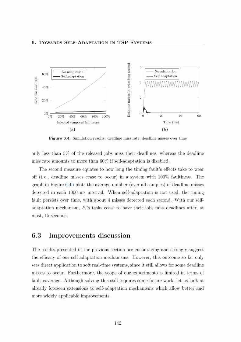
6. Towards Self-Adaptation in TSP Systems

0% 20% 40% 60% 80% 100%0%

20%

40%

60%

Injected temporal faultiness

Deadlinemissrate

No adaptationSelf adaptation

(a)

0 20 40 600

2

4

6

Time (ms)

Deadlinemissesin

precedingsecond

No adaptationSelf adaptation

(b)

Figure 6.4: Simulation results: deadline miss rate; deadline misses over time

only less than 5% of the released jobs miss their deadlines, whereas the deadline

miss rate amounts to more than 60% if self-adaptation is disabled.

The second measure equates to how long the timing fault’s effects take to wear

off (i. e., deadline misses cease to occur) in a system with 100% faultiness. The

graph in Figure 6.4b plots the average number (over all samples) of deadline misses

detected in each 1000 ms interval. When self-adaptation is not used, the timing

fault persists over time, with about 4 misses detected each second. With our self-

adaptation mechanism, P1’s tasks cease to have their jobs miss deadlines after, at

most, 15 seconds.

6.3 Improvements discussion

The results presented in the previous section are encouraging and strongly suggest

the efficacy of our self-adaptation mechanisms. However, this outcome so far only

sees direct application to soft real-time systems, since it still allows for some deadline

misses to occur. Furthermore, the scope of our experiments is limited in terms of

fault coverage. Although solving this still requires some future work, let us look at

already foreseen extensions to self-adaptation mechanisms which allow better and

more widely applicable improvements.

142

6.3 Improvements discussion

6.3.1 Multiprocessor

The results we have obtained are restricted to uniprocessor platforms. As we havestated in Section 1.3, taking advantage of multiprocessor platforms (with identicalor non-identical processors) opens room for supporting self-adaptive behavior tocope with unforeseen changes in operational and environmental conditions. Wehave described and illustrated in Section 3.2.4 the approach that we envision. Theoverall idea is to detect that the root cause of a temporal fault lies with a specificprocessor core, and perform a schedule switch that reassigns the activities of thatcore to another core; the latter, prior to that moment, can be either idle or attributedto a function which can tolerate a performance degradation for the sake of safety(e.g., a non-critical function).

6.3.2 Reconfiguration

As shown in the results, the use of self-adaptation mechanisms significantly decreasesthe number of deadline misses, when comparing to the same system execution with-out the use of such mechanisms. However, besides the good contributions to mitigatethis problem, these self-adaptation mechanisms do not cover all the possible cases,neither ensure perpetual stability of the system. For example, temporal faultinessmay further increase, due to the additional execution time provided to the faultypartition not being enough. Furthermore, this problem can be even more serious ifthe system encounters deadline misses in more than one partition.

As it is impossible to foresee all the cases, i.e., all the suitable PSTs associated todifferent temporal requirements, we need to provide ways to reconfigure the system,during its execution, when facing this kind of problems. This reconfiguration can bedone replacing the original set of PSTs by a redefined and updated set that coversthe new temporal requirements and encounters issues. Self-adaptability can, in suchmore serious scenario, provide a temporary mitigation to allow time for a moretargeted solution through online reconfiguration which enables mission survival.

We have collaborated with Rosa et al. (2011) in approaching reconfigurationin a study which, despite contemporary and related, is outside the scope of thisdissertation.

143

6. Towards Self-Adaptation in TSP Systems

6.3.3 Proactivity

The results we presented in Section 6.2.1.4, although pointing towards the advan-tages of self-adaptive behavior, are for now only directly applicable to soft real-timesystems—since they still allow for some deadline misses to occur before takingaction. To apply this approach to safety-critical systems with hard real-time work-loads, action should be taken to avoid temporal faults (Almeida et al., 2013). Forthis, it is necessary to identify patterns which indicate, with a given degree of con-fidence, that the system is behaving towards a temporal fault.

6.4 Summary

In this chapter, we have present preliminary results on self-adaptive behavior in TSPsystems, based on the monitoring and adaptation mechanisms present in the AIRarchitecture. We have proposed coping with temporal faults in TSP systems witha set of feasible and specially crafted partition scheduling tables, among which thesystem shall switch upon detecting temporal faults within a partition. The addedself-adaptability does not void the certification advantages brought by the use ofprecomputed partition schedules. The results of our experimental evaluation showthe self-adaptation to timing faults we propose achieves a degree of temporal faultcontrol suitable for soft real-time guarantees. Future work includes a more completeevaluation with a wider fault coverage, namely faults in more than one partition.Furthermore, this preliminary approach shall evolve towards a dynamic approachthat does not compromise the mission’s safety and the system’s certifiability. Otherenhancements include taking profit from multiprocessor and proactively avoid dead-line misses. The latter should lead us closer to a self-adaptation policy for hardreal-time.

144

Chapter 7

Conclusion and Future Work

In this dissertation, we have approached the problem of real-time scheduling onmulticore time- and space-partitioned (TSP) system archictures. We have proposed(Chapter 3) a system architecture (and respective formal model) for TSP systemssupport parallelism at both the application (between tasks) and system (betweenapplications) level.

We then augmented the state of the art with a formal approach, based on compo-sitional analysis, to obtain valid parameters to ensure schedulability of applications(Chapter 4); the presented approach is the first addressing the compositional analysisproblem upon a non-identical multiprocessor platform. In Section 4.3.2, we have an-alytically proven that non-identical multiprocessor platforms provide gains over iden-tical multiprocessor platforms with the same overall capacity, in terms of component-level schedulability in systems modeled as compositional scheduling frameworks; thetests we performed with randomly generated task sets (Section 4.3.4.1) confirm thisresult, which is coherent with results found in the literature for dedicated multipro-cessor platforms (Baruah & Goossens, 2008). In Section 4.4.2, we have analyticallyproven that gEDF, when used as a global-level intercomponent scheduler, does notensure that compositionality is maintained in the presence of non-identical plat-forms. We have then proposed a new scheduler, umprEDF, which guarantees thatthe resource interface of each component is respected and ensured, and composi-tionality is maintained; this is a crucial point when considering the advantage ofindependent development and verification brought by component-based approaches.

145

7. Conclusion and Future Work

Next (Chapter 5), we presented the design and development of hsSim, an object-oriented scheduling analysis, simulation and schedule generation tool; hsSim shall bemade available as an open-source tool for the real-time scheduling research commu-nity, and is a proof of concept for the inclusion of support to hierarchical schedulingin a more mature tool.1 We have used hsSim to show the formal methods we pre-sented in Chapter 4 in action.

Finally, in Chapter 6, we have presented preliminary results pertaining to self-adaptive behavior. Although preliminary, and limited in terms of assumptions, ourresults allow us to believe that, besides parallelism, the use of multiprocessor alsoenables self-adaptive behavior in TSP systems.

Given the above, we can say that the overall goals have been met: to show thatmultiprocessor platforms, in particular with non-identical processors, provide newcapabilities to time- and space-partitioned systems with respect to parallelism, andopen room for self-adaptability.

7.1 Applicability perspective

In this dissertation, we employ a system model relying on assumptions regarding thetemporal impact of hardware-related phenomena (such as bus contention, or cachememory). More specifically, we assume that this temporal impact is either negli-gible, already accounted for in the worst-case execution requirement estimations,and/or at least partially eliminated by the choice of cache managament or bus con-tention policies. This is a common assumption in real-time scheduling research, andnot so far from reality as it may seem. For instance, Jalle et al. (2013) experimen-tally show that the two most-used policies to manage bus contention (Time-DivisionMultiple Access and Interference-Aware Bus Arbitrer) observe time composability—that is, worst-case execution requirement estimations obtained for one task in isola-tion (taking into account the bus contention control policy) hold when it is put tocontend for bus access with other tasks (regardless of the characteristics of the lat-ter). In a study commissioned by the European Aviation Safety Agency, Jean et al.(2012) recommend that the approach to multicore processors in airborne systemsuses hardware-based cache partitioning mechanisms.

1https://code.google.com/p/hssim.

146

7.1 Applicability perspective

Over the years, there were research projects funded by European entities (mostnotably the European Commission and the European Space Agency) employingcomponent-based approaches and/or time and space partitioning to achieve archi-tectural hybridization or to cope with mixed-criticality systems. In some of theseprojects, mostly contemporary with the hereby presented work, multicore processorshave been approached to some extent.

• The ACTORS project2 (2008–2011) employed reservation-based schedulingto enforce dependability and predictability over multicore embedded systems.Bini et al. (2011b) describe the approach (based on compositional analysis withBini et al. (2009b)’s Multi Supply Function abstraction) and implementationinto the Linux kernel (based on Abeni & Buttazzo (1998)’s Constant Band-width Server); their approach is limited to partitioned local-level scheduling.Bini et al. (2011a) describe an approach to use with global local-level schedul-ing algorithms (based on compositional analysis with Bini et al. (2009a)’sParallel Supply Function), which was however not successfully demonstrated.

• The RECOMP project3 (2010–2013) aimed at enabling component-based de-velopment of mixed-criticality systems on multicore platforms. Low experiencewith hierarchical scheduling is pointed out as one of the obstacles to certify-ing safety-critical applications on multicores, and the work of Easwaran et al.(2009b) (which we have extended towards non-identical multiprocessors) is de-scribed as fulfilling several of the project’s requirements (RECOMP, 2011a).The approach to multicore followed in the RECOMP project is that of havingmultiple interconnected nodes, each of them working on one single processor(akin to the approach pictured in Figure 3.3a) (RECOMP, 2011b, 2013).

• In the KARYON project4 (2011—), architectural hybridization is proposedto cope with the risks of cooperating in an uncertain environment, and timeand space partitioning is proposed as a way of implementing such architecture(Nóbrega da Costa et al., 2013).

2Adaptivity and Control of Resources in Embedded Systems, http://www.actors-project.eu/3Reduced Certification Costs Using Trusted Multi-core Platforms, http://atcproyectos.ugr.es/

recomp/4Kernel-Based ARchitecture for safetY-critical cONtrol, http://www.karyon-project.eu/

147

7. Conclusion and Future Work

The work presented in this dissertation is applicable to the architectures consid-ered in or resulting from the aforementioned projects, even addressing issues leftopen at the end of some of them. Most notably, our results go beyond the achieve-ments of these projects with respect to intrapartiton parallelism and to the usenon-identical processors. We believe this is the first step towards breaking the vi-cious cycle between the hardware and software support to non-identical processors.In the aerospace domain, the widely used SPARC LEON processors allow hetero-geneous multicore configurations, but the lack of operating system support theretodisencourages its use.5

Besides the initially established main focus on safety-critical application domains,our results also contribute towards the formal verification of component-based sys-tems supported on non-identical multiprocessors platforms such as Cell (Gschwindet al., 2006) and big.LITTLE—namely the big.LITTLEMP use model (Greenhalgh,2011). Although these multiprocessors are not typically employed in safety-criticaldomains, applying a component-based approach to the development of complex soft-ware to run on them allows reducing the complexity and cost of the latter, whilesecuring that individual components achieve a minimum quality of service. Thisshall be particularly true as operating system support to hierarchical schedulingincreases; for instance, Abdullah et al. (2013) are starting to implement virtual-clustered multiprocessor scheduling (Easwaran et al., 2009b) in the Linux kernel.

7.2 Future work

Although our goals have been met, the work presented here is only a fraction of awider work concerning the industrial adoption of systems based on the architecturedesign we consider. Most notably, the various constraints inherent to the scope ofa PhD prevented improving the analysis by lifting system model assumptions thatseparate it from real systems (namely aspects related to multiprocessor hardware)and validating the work with a prototype implementation of a multiprocessor TSPsystem on real hardware. The lack of real or realistic case studies, endemic to thereal-time systems and cyber-physical systems community (Di Natale et al., 2013),

5http://comments.gmane.org/gmane.comp.hardware.opencores.leon-sparc/14873.

148

7.2 Future work

has also been an obstacle to the full expression of this work, circumvented to thepossible extent through the use of synthetic workloads.

The project READAPT (Reconfigurability and Adaptability in Safe and SecureMulticore Architectures for Mixed-Criticality Applications) was approved for fundingby Fundação para a Ciência e a Tecnologia (FCT, the Portuguese national sciencefoundation), and began near the conclusion of the work described in this disserta-tion.6 In READAPT, the LaSIGE team collaborates with the industrial partnerGMV. This project will hopefully provide the necessary means to bring the herebypresented results into real practice, and to pursue other related work. Collaborationswith international partners from both academia and industry have been proposed,and some more are being prepared at the time of this writing. We are for this reasonoptimistic that we will have great opportunities to continue, improve and expandthe work presented here. We now list some of the open issues and topics to address.

7.2.1 Hardware support and system model assumptions

As mentioned before, our a system model is limited by assumptions regarding thetemporal impact of hardware-related phenomena (such as bus contention, or cachememory). Although finding echo in real requirements, this surely limits the appli-cability of our results. In the future, we aim to take these phenomena into specificaccount when analyzing TSP systems.

Another hardware-related aspect worth investigating in the future is that ofevaluating the power consumption trade-off between TSP systems based on identicalmultiprocessors and those bases on non-identical multiprocessors.

7.2.2 Scheduling algorithms

In Chapter 4, we have analyzed compositional scheduling frameworks assuming agEDF local-level scheduling algorithm. Since the divisions of tasks into componentsmay be functional or institutional in nature, it is not guaranteed that the “Dhall& Liu (1978) effect” of which gEDF suffers is eliminated. As we have seen in Sec-tion 2.2.3, hybrid variants of gEDF have been proposed to cope with this effect,

6http://www.navigators.di.fc.ul.pt/wiki/Project:READAPT.

149

7. Conclusion and Future Work

without incurring the typically higher number of preemptions of the LLF algorithm;these variants include EDZL (Lee, 1994).

However, we have found (Craveiro & Rufino, 2013) that, when there are timeintervals at which the processing platform is partially or totally unavailable to thescheduler, EDZL is not appropriate. The reason for this is that the scheduler com-pares the laxity of the jobs to a constant value (zero) without regard for the expectedavailability of the platform. We have shown a proof of concept for the general ideaof a possible solution, using a simple resource model and comparing the laxity ofthe jobs against a non-zero value obtained from the resource interface; our proof ofconcept shares some characteristics with Davis & Kato (2012)’s Fixed Priority untilStatic Laxity algorithm.

Our intuition is that the solution for this problem may be based on an adaptednotion of laxity that considers the difference between how much execution capacityone single job can have available until its deadline (according to the resource in-terface) and its remaining execution. Open questions with respect to this probleminclude the dynamics of this laxity and schedulability analysis when scheduling oc-curs upon a multiprocessor reservation according to the resource models proposed inthe literature (Bini et al., 2009a; Burmyakov et al., 2012; Craveiro & Rufino, 2012;Lipari & Bini, 2010; Shin et al., 2008).

7.2.3 Compositional analysis

Although compositional analysis is applied to systems which are motivated by thecoexistence of heterogeneous workloads, the vast majority of works on compositionalanalysis (including the work presented in Chapter 4 of this dissertation) assume hardreal-time tasks only. In the near future, we aim to approach compositional analysison systems models contemplating soft real-time and mixed-criticality. To the best ofour knowledge, only Leontyev & Anderson (2009) approach compositional analysison a hierarchical scheduling framework where components may have soft real-timeworkloads, on identical multiprocessors; however, the resource provision is hard (i.e.,it must be guaranteed). We aim to provide soft resource provisions for soft real-timeworkloads.

150

7.2 Future work

7.2.4 Reconfiguration and proactivity

As seen in Section 6.3.3, improving the survivability of space vehicles requires notonly reacting to abnormal events but also proactively tolerating their occurrence(Almeida et al., 2013). Performing proactive fault-tolerance actions implies forecast-ing and preventing future uncontrolled abnormal events. With respect to proactivefault tolerance in TSP systems, a set of statistically significant patterns of inter-est should be usable as key indicators for forecasting the system’s behavior. Suchindicators shall assist the detection of a potentially anomalous situation, i.e. animminent failure.

The use of multiprocessor platforms is TSP sytstems that we defend in our thesisbrings added value to proactive fault tolerance. For instance, we can have one ormore spare processor cores that take over the duties of cores which present evidenceof an imminent failure— thus avoiding more severe faults before they happen.

151

References

Abdullah, S.M.J., Khalilzad, N.M., Behnam, M. & Nolte, T. (2013). To-wards implementation of virtual-clustered multiprocessor scheduling in Linux. In8th IEEE International Symposium on Industrial Embedded Systems (SIES 2013)Work-in-Progress session, Porto, Portugal. xix, 148

Abeni, L. & Buttazzo, G. (1998). Integrating multimedia applications in hardreal-time systems. In 19th IEEE Real-Time Systems Symposium (RTSS ’98), 4–13, Madrid, Spain. xiv, xv, 2, 9, 31, 109, 147

AEEC (1991). Design guidance for Integrated Modular Avionics. ARINC Report651, Airlines Electronic Engineering Committee (AEEC), initial release (currentrevision: 651-1, November 1997). xiv, 2

AEEC (1997). Avionics application software standard interface. ARINC Specifi-cation 653, Airlines Electronic Engineering Committee (AEEC), initial release(current revision: 653P1-3, November 2010). xiv, 2, 3, 4, 5, 33, 49, 51, 59, 61, 132

AEEC (2007). Avionics application software standard interface. ARINC Specifica-tion 653 Part 2 (Extended Services), Airlines Electronic Engineering Committee(AEEC), initial release (current revision: 653P2-3, June 2012). 4, 51, 133

Almeida, K., Pinto, R.C. & Rufino, J. (2013). Fault detection in time- andspace-partitioned systems. In INFORUM 2013—Simpósio de Informótica, Évora,Portugal. 144, 151

Anderson, J., Baruah, S. & Brandenburg, B. (2009). Multicore operating-system support for mixed criticality. In CPS Week 2009 Workshop on Mixed Crit-icality , San Francisco, CA, USA. xv, 7

153

REFERENCES

Andersson, J., Gaisler, J. & Weigand, R. (2010). Next generation multipur-pose microprocessor. In DASIA 2010 “DAta Systems In Aerospace” Conference,Budapest, Hungary. xv, 7

Audsley, N. & Wellings, A. (1996). Analysing APEX applications. In 17thIEEE Real-Time Systems Symposium (RTSS ’96), 39–44, Washington, DC, USA.xiv, 3, 33, 34, 35

Audsley, N., Burns, A., Richardson, M., Tindell, K. & Wellings, A.

(1993). Applying new scheduling theory to static priority pre-emptive scheduling.Software Engineering Journal , 8(5):284–292. 21

Audsley, N.C., Burns, A., Davis, R.I., Tindell, K.W. & Wellings, A.J.

(1995). Fixed priority pre-emptive scheduling: An historical perspective. Real-Time Systems , 8(2):173–198. 14

AUTOSAR (2006). Technical overview, v2.0.1. 6

AUTOSAR (2013a). Requirements on operating system, v3.1.0, release 4.1, revision1. 7, 8

AUTOSAR (2013b). Specification of operating system, v5.1.0, release 4.1, revision1. 7, 8

Baker, T.P. (2003). Multiprocessor EDF and Deadline Monotonic schedulabil-ity analysis. In 24th IEEE Real-Time Systems Symposium (RTSS ’03), Cancun,Mexico. v, 25, 26, 28, 43, 76

Baker, T.P. & Baruah, S.K. (2007). Schedulability analysis of multiprocessorsporadic task systems. In I. Lee, J.Y.T. Leung & S.H. Son, eds., Handbook ofReal-Time and Embedded Systems , chap. 3, Chapman & Hall/CRC. 22, 25

Baruah, S. (2007). Techniques for multiprocessor global schedulability analysis. In28th IEEE Real-Time Systems Symposium (RTSS ’07), Tucson, AZ, USA. 25, 26,27, 43, 44

154

REFERENCES

Baruah, S. & Goossens, J. (2008). The EDF scheduling of sporadic task systemson uniform multiprocessors. In 29th IEEE Real-Time Systems Symposium (RTSS’08), Barcelona, Spain. xvii, 11, 28, 76, 77, 78, 80, 81, 84, 87, 91, 145

Baruah, S., Goossens, J. & Lipari, G. (2002). Implementing constant-bandwidth servers upon multiprocessor platforms. In 8th IEEE Real-Time andEmbedded Technology and Applications Symposium (RTAS ’02), 154–163, SanJose, CA, USA. 31

Baruah, S., Bonifaci, V., Marchetti-Spaccamela, A. & Stiller, S. (2009).Implementation of a speedup-optimal global EDF schedulability test. In 21st Eu-romicro Conference on Real-Time Systems (ECRTS ’09), Dublin, Ireland. 46

Baruah, S.K. (2004). Optimal utilization bounds for the fixed-priority schedul-ing of periodic task systems on identical multiprocessors. IEEE Transactions onComputers , 53(6):781–784. 27

Baruah, S.K., Mok, A.K. & Rosier, L.E. (1990). Preemptively scheduling hard-real-time sporadic tasks on one processor. In 11th Real-Time Systems Symposium(RTSS ’90), Lake Buena Vista, Florida, USA. 21

Bertogna, M., Cirinei, M. & Lipari, G. (2005). Improved schedulability anal-ysis of EDF on multiprocessor platforms. In 17th Euromicro Conference on Real-Time Systems (ECRTS ’05), 209–218, Palma de Mallorca, Spain. 26, 43, 46

Bini, E. & Lipari, G. (2011). Introduction to the special issue. ACM SIGBEDReview , 8(1), Special Issue on 3rd Workshop on Compositional Theory and Tech-nology for Real-Time Embedded Systems (CRTS 2010). 35

Bini, E., Buttazzo, G. & Buttazzo, G. (2003). Rate monotonic analysis: thehyperbolic bound. IEEE Transactions on Computers , 52(7):933 – 942. 21

Bini, E., Bertogna, M. & Baruah, S. (2009a). Virtual multiprocessor platforms:Specification and use. In 30th IEEE Real-Time Systems Symposium (RTSS ’09),437–446, Washington, DC, USA. 14, 46, 47, 51, 147, 150

155

REFERENCES

Bini, E., Buttazzo, G. & Bertogna, M. (2009b). The multi supply functionabstraction for multiprocessors. In 15th IEEE International Conference on Embed-ded and Real-Time Computing Systems and Applications (RTCSA 2009), 294–302,Beijing, China. 45, 46, 51, 147

Bini, E., Buttazzo, G. & Bertogna, M. (2011a). Multicore. Deliverable D4d,ACTORS project. 147

Bini, E., Buttazzo, G., Eker, J., Schorr, S., Guerra, R., Fohler, G.,

Årzén, K.E., Romero, V. & Scordino, C. (2011b). Resource managementon multi-core systems: the ACTORS approach. IEEE Micro, 31(3):72–81. xix,147

Binns, P. (2001a). A robust high-performance time partitioning algorithm: theDigital Engine Operating System (DEOS) approach. In 20th IEEE/AIAA DigitalAvionics Systems Conference (DASC 2001), Daytona Beach, FL, USA. 50

Binns, P.A. (2001b). Slack scheduling for improved response times of period trans-formed processes. Patent, US 6189022. 50

Black, R. & Fletcher, M. (2006). Open Systems Architecture - Both Boon andBane. In 25th IEEE/AIAA Digital Avionics Systems Conference (DASC 2006), 1–7. xiv, 5

Brocal, V., Masmano, M., Ripoll, I., Crespo, A., Balbastre, P. &

Metge, J.J. (2010). Xoncrete: a scheduling tool for partitioned real-time sys-tems. In Embedded and Real Time Software and Systems (ERTS2 2010), Toulouse,France. 54

Burmyakov, A., Bini, E. & Tovar, E. (2012). The Generalized MultiprocessorPeriodic Resource interface model for hierarchical multiprocessor scheduling. InRTNS ’12 , Pont à Mousson, France. 150

Buttazzo, G., Bini, E. & Wu, Y. (2010). Partitioning parallel applications onmultiprocessor reservations. In 22nd Euromicro Conference on Real-Time Systems(ECRTS ’10), 24–33, Brussels, Belgium. 46

156

REFERENCES

Buttazzo, G., Bini, E. & Wu, Y. (2011). Partitioning real-time applications overmulticore reservations. IEEE Transactions on Industrial Informatics , 7(2):302–315. 46

Buttazzo, G.C. (1997). Hard Real-Time Computing Systems: Predictable Schedul-ing Algorithms and Applications . Real-Time Systems, Kluwer Academic Publish-ers, Boston / Dordrecht / London. 14, 30

Buttazzo, G.C. (2005). Rate Monotonic vs. EDF: Judgment Day. Real-Time Sys-tems , 29:5–26, 10.1023/B:TIME.0000048932.30002.d9. 25

Carpenter, J., Funk, S., Holman, P., Anderson, J. & Baruah, S. (2004).A categorization of real-time multiprocessor scheduling problems and algorithms.In J.Y.T. Leung, ed., Handbook on Scheduling: Algorithms, Methods, and Models ,Chapman & Hall/CRC. 14, 18

Coronel, J. & Crespo, A. (2012). Design of the generic virtualization layer.Deliverable D3.3, MultiPARTES project. 51

Coutinho, M., Almeida, C. & Rufino, J. (2006). VITRAL - a text mode win-dow manager for real-time embedded kernels. In 11th IEEE International Con-ference on Emerging Technologies and Factory Automation (ETFA 2006), 1254–1260, Prague, Czech Republic. 135

Craveiro, J., Rufino, J., Schoofs, T. & Windsor, J. (2009). Flexible oper-ating system integration in partitioned aerospace systems. In INForum 2009—Simpósio de Informática, 49–60, Lisbon, Portugal. 59

Craveiro, J., Rufino, J. & Singhoff, F. (2011). Architecture, mechanisms andscheduling analysis tool for multicore time- and space-partitioned systems. ACMSIGBED Review , 8(3):23–27, special issue of the 23rd Euromicro Conference onReal-Time Systems (ECRTS ’11) Work-in-Progress session. 51, 53

Craveiro, J.P. & Rufino, J. (2012). Towards compositional hierarchical schedul-ing frameworks on uniform multiprocessors. Tech. Rep. TR-2012-08, Universityof Lisbon, DI–FCUL, revised January 2013. 150

157

REFERENCES

Craveiro, J.P. & Rufino, J. (2013). Global laxity-based scheduling on multi-processor resource reservations. In 4th International Real-Time Scheduling OpenProblems Seminar (RTSOPS 2013), Paris, France. 150

Craveiro, J.P.G.C. (2009). Integration of generic operating systems in partitionedarchitectures . Master’s thesis, Faculty of Sciences, University of Lisbon, Lisbon,Portugal. 59, 129

Davis, R.I. & Burns, A. (2009). Priority assignment for global fixed priority pre-emptive scheduling in multiprocessor real-time systems. In 30th IEEE Real-TimeSystems Symposium (RTSS ’09), 398–409, Washington, DC, USA. 88

Davis, R.I. & Burns, A. (2011). A survey of hard real-time scheduling for multi-processor systems. ACM Computing Surveys , 43(4):35:1–35:44. 14, 18

Davis, R.I. & Kato, S. (2012). FPSL, FPCL and FPZL schedulability analysis.Real-Time Systems , 48(6):750–788. 150

DDC-I (2012). Deos: A Time & Space Partitioned DO-178B Level A certifica-ble RTOS. Fact sheet, DDC-I, http://www.ddci.com/product_fact_sheets/Deos.pdf. Retrieved on July 31, 2013. 50

de la Puente, J.A., Balbastre, P. & Garrido, J. (2012). Scheduling parti-tioned systems on multicore platforms. Deliverable D3.2, MultiPARTES project.51

Deng, Z. & Liu, J.W.S. (1997). Scheduling real-time applications in an openenvironment. In 18th IEEE Real-Time Systems Symposium (RTSS ’97), 308–319.32

Deng, Z., Liu, J.S. & Sun, J. (1997). A scheme for scheduling hard real-timeapplications in open system environment. In 9th Euromicro Workshop on Real-Time Systems (RTS 1997), 191–199. 32

Dertouzos, M.L. (1974). Control robotics: The procedural control of physicalprocesses. In Information Processing 74: Proceedings of IFIP Congress 74 , 807–813, Stockholm, Sweden. 21, 22

158

REFERENCES

Dertouzos, M.L. & Mok, A.K. (1989). Multiprocessor online scheduling of hard-real-time tasks. IEEE Transactions on Software Engineering , 15(12):1497–1506.21, 22

Dhall, S.K. & Liu, C.L. (1978). On a real-time scheduling problem. OperationsResearch, 26(1):127–140. 22, 24, 27, 124, 149

Di Natale, M., Dong, C. & Zeng, H. (2013). Reality check: the need for bench-marking in RTS and CPS. In 4th International Real-Time Scheduling Open Prob-lems Seminar (RTSOPS 2013), Paris, France. 148

Easwaran, A., Shin, I., Sokolsky, O. & Lee, I. (2006). Incremental schedu-lability analysis of hieararchical real-time components. In 6th International Con-ference on Embedded Software (EMSOFT ’06), Seoul, Korea. xvi, 9

Easwaran, A., Anand, M. & Lee, I. (2007). Compositional analysis frameworkusing EDP resource models. In 28th IEEE Real-Time Systems Symposium (RTSS’07), Tucson, AZ, USA. 41, 53, 109

Easwaran, A., Lee, I., Sokolsky, O. & Vestal, S. (2009a). A compositionalscheduling framework for digital avionics systems. In 15th IEEE InternationalConference on Embedded and Real-Time Computing Systems and Applications(RTCSA 2009), Beijing, China. 41, 53

Easwaran, A., Shin, I. & Lee, I. (2009b). Optimal virtual cluster-based multi-processor scheduling. Real-Time Systems , 43:25–59. xvii, xiv, 11, 42, 43, 44, 46,73, 74, 75, 84, 85, 86, 88, 91, 95, 147, 148

Feng, X.A. & Mok, A.K. (2002). A model of hierarchical real-time virtual re-sources. In 23rd IEEE Real-Time Systems Symposium (RTSS ’02), 26–35, Austin,TX, USA. 40

Fletcher, M. (2009). Progression of an open architecture: from Orion to Altairand LSS. Tech. rep., Honeywell International. xiv, 5

Fortescue, P.W., Stark, J.P.W. & Swinerd, G., eds. (2003). Spacecraft Sys-tems Engineering . Wiley, 3rd edn. 133

159

REFERENCES

Fuchsen, R. (2010). How to address certification for multi-core based IMA plat-forms: current status and potential solutions. In 29th IEEE/AIAA Digital Avion-ics Systems Conference (DASC 2010), 5.E.3–1–5.E.3–11, Salt Lake City, UT. 7

Funk, S., Goossens, J. & Baruah, S. (2001). On-line scheduling on uniformmultiprocessors. In 22nd IEEE Real-Time Systems Symposium (RTSS ’01), Lon-don, UK. 28, 88, 104

Gamma, E., Helm, R., Johnson, R. & Vlissides, J. (1997). Design Patterns:Elements of Reusable Object-Oriented Software. Addison-Wesley. 108, 110, 113,117

Gaudel, V., Singhoff, F., Plantec, A., Dissaux, P. & Legrand, J. (2013).Composition of design patterns : from the modeling of RTOS synchronizationtools to schedulability analysis. In The 3rd Embedded Operating Systems Workshop(EWiLi’13), Toulouse, France. 117

Goossens, J., Funk, S. & Baruah, S. (2003). Priority-driven scheduling ofperiodic task systems on multiprocessors. Real Time Systems , 25(2–3):187–205.25

Greenhalgh, P. (2011). big.LITTLE processing with ARM Cortex-A15 & Cortex-A7. White paper, ARM Ltd. 148

Gschwind, M., Hofstee, H.P., Flachs, B., Hopkins, M., Watanabe, Y.

& Yamazaki, T. (2006). Synergistic processing in Cell’s multicore architecture.IEEE Micro, 26(2):10–24. 148

Hausmans, J.P.H.M., Geuns, S.J., Wiggers, M.H. & Bekooij, M.J.G.

(2012). Compositional temporal analysis model for incremental hard real-time sys-tem design. In 12th International Conference on Embedded Software (EMSOFT’12), Tampere, Finland. xvi, 9

Hodson, R. & Ng, T. (2007). Avionics for exploration. In NASA Technology Ex-change Conference, Galveston, TX, USA. xiv, 5

160

REFERENCES

Holenderski, M., Bril, R.J. & Lukkien, J.J. (2013). Grasp: Visualizing thebehavior of hierarchical multiprocessor real-time systems. Journal of Systems Ar-chitecture, 59(6):307–314, available online: July 17, 2012. 52, 119

Howard, C.E. (2011). RTOS for a software-driven world. Military & AerospaceElectronics , 22(3), http://www.militaryaerospace.com/articles/print/volume-22/issue-30/technology-focus/rtos-for-a-software-driven-world.html. Retrieved onJuly 31, 2013. 50, 52

Jalle, J., Abella, J., Quiñones, E., Fossati, L., Zulianello, M. & Ca-

zorla, F.J. (2013). Deconstructing bus access control policies for real-time mul-ticores. In 8th IEEE International Symposium on Industrial Embedded Systems(SIES 2013), Porto, Portugal. xviii, 146

Jean, X., Gatti, M., Berthon, G. & Fumey, M. (2012). MULCORS - the useof multicore procesors in airborne systems. Dossier CCC/12/006898 - Rev. 07,Thales Avionics / European Aviation Safety Agency. xviii, 146

Julliand, J., Mountassir, H. & Oudot, E. (2007). Composability, compat-ibility, compositionality: automatic preservation of timed properties during in-cremental development. Research Report 2007–01, Laboratoire d’Informatique del’Université de Franche–Comté, Besançon, France. 35

Kaiser, R. & Wagner, S. (2007a). Evolution of the PikeOS microkernel. In I. Kuz& S.M. Petters, eds., 1st Int. Workshop on Microkernels for Embedded Systems(MIKES 2007), 50–57, Sydney, Australia. 49

Kaiser, R. & Wagner, S. (2007b). The PikeOS concept: History anddesign. White paper, SYSGO, http://www.sysgo.com/nc/en/products/document-center/whitepapers/the-pikeos-concept-history-and-design/. Re-trieved on July 31, 2013. 49

King, T. (2011). Slack scheduling enhances multicore performance in safety-criticalapplications. EDN , http://www.edn.com/design/systems-design/4368338/Slack-scheduling-enhances-multicore-performance-in-safety-critical-applications/.Retrieved on July 31, 2013. 50

161

REFERENCES

King, T. (2013). Cache partitioning increases CPU utilization for safety-critical multicore applications.Military Embedded Systems , http://mil-embedded.com/articles/cache-utilization-safety-critical-multicore-applications/. Retrievedon July 31, 2013. 50

Kopetz, H. (1997). Real-Time Systems: Design Principles for Distributed Em-bedded Applications . Real-Time Systems, Kluwer Academic Publishers, Boston /Dordrecht / London. xiii, 1, 14

Kuo, T.W. & Li, C.H. (1999). A fixed-priority-driven open environment for real-time applications. In 20th IEEE Real-Time Systems Symposium (RTSS ’99), 256–267. 32, 33

Kuo, T.W., Lin, K.J. & Wang, Y.C. (2000). An open real-time environment forparallel and distributed systems. In 20th International Conference on DistributedComputing Systems (ICDCS 2000), 206 –213. 33

Lackorzyński, A., Warg, A., Völp, M. & Härtig, H. (2012). Flatteninghierarchical scheduling. In 12th International Conference on Embedded Software(EMSOFT ’12), Tampere, Finland. xv, 9

Lauzac, S., Melhem, R. & Mossé, D. (1998). An efficient RMS admission controland its application to multiprocessor scheduling. In 12th Int. Parallel ProcessingSymposium / 9th Symposium on Parallel and Distributed Processing (IPPS/SPDP’98), 511–518. 21

Lee, S.K. (1994). On-line multiprocessor scheduling algorithms for real-time tasks.In IEEE Region 10’s Ninth Annual International Conference (TENCON’94), 607–611. 27, 150

Lee, Y., Kim, D., Younis, M. & Zhou, J. (1998). Partition scheduling in APEXruntime environment for embedded avionics software. In 5th International Confer-ence on Real-Time Computing Systems and Applications (RTCSA 1998), 103–109,Hiroshima, Japan. 34, 35, 39

Lehoczky, J. (1990). Fixed priority scheduling of periodic task sets with arbitrarydeadlines. In 11th Real-Time Systems Symposium (RTSS ’90), 201–209. 21, 34

162

REFERENCES

Lehoczky, J.P., Sha, L. & Strosnider, J.K. (1987). Enhanced aperiodic re-sponsiveness in hard real-time environments. In 8th Real-Time Systems Sympo-sium (RTSS ’87), 261–270, San Jose, CA, USA. 30

Leontyev, H. & Anderson, J. (2009). A hierarchical multiprocessor bandwidthreservation scheme with timing guarantees. Real-Time Systems , 43:60–92. 150

Leung, J.Y.T. & Whitehead, J. (1982). On the complexity of fixed-priorityscheduling of periodic, real-time tasks. Performance Evaluation, 2(4):237–250.21, 24

Lipari, G. (2012). Software and academic research: are we going in the right di-rection? Panel presentation at the 3rd International Workshop on Analysis Toolsand Methodologies for Embedded and Real-time Systems (WATERS 2012), Pisa,Italy, http://retis.sssup.it/waters2012/accepted/panel.pdf. Retrieved on July 31,2013. 107

Lipari, G. & Baruah, S.K. (2000). Efficient scheduling of real-time multi-taskapplications in dynamic systems. In 6th IEEE Real-Time Technology and Appli-cations Symposium (RTAS ’00), 166–175, Washington , DC, USA. 33

Lipari, G. & Bini, E. (2010). A framework for hierarchical scheduling on multi-processors: From application requirements to run-time allocation. In 31st IEEEReal-Time Systems Symposium (RTSS ’10), 249 –258. 46, 47, 48, 51, 105, 150

Lipari, G. & Buttazzo, G.C. (1999). Scheduling real-time multi-task applicationsin an open system. In 11th Euromicro Workshop on Real-Time Systems (RTS1999), York, UK. 33

Lipari, G., Gai, P., Trimarchi, M., Guidi, G. & Ancilotti, P. (2005). Ahierarchical framework for component-based real-time systems. Electronic Notesin Theoretical Computer Science, 116:253–266, International Workshop on Testand Analysis of Component Based Systems (TACoS 2004). xiii, 2

Little, R. (1991). Advanced avionics for military needs. Computing and ControlEngineering Journal , 2(1):29–34. 3

163

REFERENCES

Liu, C.L. (1969). Scheduling algorithms for multiprocessors in a hard real-timeenvironment. JPL Space Programs Summary , 37(60):28–31. 14

Liu, C.L. & Layland, J.W. (1973). Scheduling algorithms for multiprogrammingin a hard-real-time environment. Journal of the ACM , 20(1):46–61. 14, 20, 21

Lorente, J.L., Lipari, G. & Bini, E. (2006). A hierarchical scheduling model forcomponent-based real-time systems. In 20th International Parallel and DistributedProcessing Symposium (IPDPS 2006), Rhodes Island, Greece. xiii, 2, 5

Lupu, I., Courbin, P., George, L. & Goossens, J. (2010). Multi-criteria eval-uation of partitioning schemes for real-time systems. In 15th IEEE InternationalConference on Emerging Technologies and Factory Automation (ETFA 2010),Bilbao, Spain. 21, 23

Masmano, M., Ripoll, I. & Crespo, A. (2005). An overview of the XtratuMnanokernel. In 1st International Workshop on Operating System Platforms forEmbedded Real-Time Applications (OSPERT 2005), Palma de Mallorca, Spain.50

Masmano, M., Ripoll, I., Crespo, A., Arberet, P. & Metge, J.J. (2009).XtratuM: an open source hypervisor for TSP embedded systems in aerospace. InDASIA 2009 “DAta Systems In Aerospace” Conference, Istanbul, Turkey. 50

Masmano, M., Ripoll, I., Crespo, A. & Peiro, S. (2010). XtratuM for LEON3:an open source hypervisor for high integrity systems. In Embedded and Real TimeSoftware and Systems (ERTS2 2010), Toulouse, France. 51

Matsubara, Y., Sano, Y., Honda, S. & Takada, H. (2012). An open-sourceflexible scheduling simulator for real-time applications. In 15th International Sym-posium on Object/Component/Service-Oriented Real-Time Distributed Computing(ISORC 2012), Shenzhen, China. 54

McConnel, T. (2010). Embedded World—PikeOS 3.1 supports mul-ticore. EE Times , http://www.eetimes.com/electronics-news/4136859/EMBEDDED-WORLD--PikeOS-3-1-supports-multicore. Retrieved on July31, 2013. 49

164

REFERENCES

Mercer, C.W., Savage, S. & Tokuda, H. (1993). Processor capacity reserves formultimedia operating systems. Tech. Rep. CMU-CS-93-157, School of ComputerScience, Carnegie Mellon University, Pittsburgh, PA, USA. 29

Mignolet, J.Y. & Wuyts, R. (2009). Embedded multiprocessor systems-on-chipprogramming. IEEE Software, 26(3):34–41. 7

Mok, A. (1983). Fundamental design problems of distributed systems for the hard-real-time environment . Ph.D. thesis, Massachusetts Institute of Technology, De-partment of Electrical Engineering and Computer Science, Cambridge, MA. 15,22

Mok, A.K. & Feng, A.X. (2002). Real-time virtual resource: A timely abstrac-tion for embedded systems. In A.L. Sangiovanni-Vincentelli & J. Sifakis, eds.,2nd International Conference on Embedded Software (EMSOFT’02), vol. 2491 ofLecture Notes In Computer Science, 182–196, Springer-Verlag, London, UK. xv,9

Mok, A.K., Feng, X.A. & Chen, D. (2001). Resource partition for real-time sys-tems. In IEEE Real-Time Technology and Applications Symposium (RTAS ’01),75–84, Taiwan, ROC. 37, 38, 39, 45, 68

Nguyen, V., Deeds-Rubin, S. & Tan, T. (2007). A SLOC counting standard. InThe 22nd Int. Ann. Forum on COCOMO and Systems/Software Cost Modeling ,Los Angeles, USA. 136

Nikolic, B., Awan, M.A. & Petters, S.M. (2011). SPARTS: Simulator forPower Aware and Real-Time Systems. In 8th IEEE International Conference onEmbedded Software and Systems (ICESS-11), Changsha, China. 112

Nóbrega da Costa, P., Craveiro, J.P., Casimiro, A. & Rufino, J. (2013).Safety kernel for cooperative sensor-based systems. In Safecomp 2013 Workshop onArchitecting Safety in Collaborative Mobile Systems (ASCoMS), Toulouse, France.147

Parkinson, P. (2011). Safety, security and multicore. In C. Dale & T. Anderson,eds., Advances in Systems Safety , 215–232, Springer London. 7

165

REFERENCES

Patterson, D. (2010). The trouble with multi-core. IEEE Spectrum, 47(7):24–29.7

Patterson, D.A. & Hennessy, J.L. (2009). Computer Orgnaization and Design:the Hardware/Software Interface. Morgan Kaufmann, Burlington, MA, USA, 4thedn. xv, 7, 61

Penix, J., Visser, W., Engstrom, E., Larson, A. & Weininger, N. (2000).Verification of time partitioning in the DEOS scheduler kernel. In 22nd Interna-tional Conference on Software engineering , 488–497, Limerick, Ireland. 50

Phan, L.T.X., Lee, J., Easwaran, A., Ramaswamy, V., Lee, I. & Sokolsky,

O. (2011). CARTS: A tool for compositional analysis of real-time systems. ACMSIGBED Review , 8(1), Special Issue on 3rd Workshop on Compositional Theoryand Technology for Real-Time Embedded Systems (CRTS 2010). 53

Phillips, C.A., Stein, C., Torng, E., & Wein, J. (2002). Optimal time-criticalscheduling via resource augmentation. Algorithmica, 32(2):163–200. 105

Planche, L. (2008). Analysis of the application of the ARINC653 standard tospace systems. Tech. Rep. ASG7.TN.12311.ASTR, EADS Astrium. xiv, 6

Plancke, P. & David, P. (2003). Technical note on on-board computer anddata systems. European Space Technology Harmonisation, Technical Dossier onMapping, Technical Note TOS-ES/651.03/PP, ESA. xiv, 6

RECOMP (2011a). Component model specification. Deliverable D2.1, RECOMPproject. 147

RECOMP (2011b). Operating system support for safe multi-core integration: Ar-chitecture, implementation, evaluation. Deliverable D3.3, RECOMP project. 49,147

RECOMP (2013). HW support for operating systems, applications and monitoring.Deliverable D3.4, RECOMP project. 147

166

REFERENCES

Rosa, J., Craveiro, J. & Rufino, J. (2011). Safe online reconfiguration of time-and space-partitioned systems. In 9th IEEE International Conference on Indus-trial Informatics (INDIN 2011), Caparica, Lisbon, Portugal. 59, 143

Rufino, J., Filipe, S., Coutinho, M., Santos, S. & Windsor, J. (2007).ARINC 653 interface in RTEMS. In DASIA 2007 “DAta Systems In Aerospace”Conference, Naples, Italy. 57

Rufino, J., Craveiro, J. & Verissimo, P. (2010). Architecting robustness andtimeliness in a new generation of aerospace systems. In A. Casimiro, R. de Lemos& C. Gacek, eds., Architecting Dependable Systems VII , vol. 6420 of Lecture Notesin Computer Science, 146–170, Springer Berlin / Heidelberg. 57, 58

Rufino, J., Craveiro, J., Schoofs, T., Cristóvão, J. & Tatibana, C.

(2011). AIR: Technology innovation for future spacecraft onboard computing sys-tems. In International Conference on Computer as a Tool (EUROCON 2011),Lisbon, Portugal. 135

Rushby, J. (1999). Partitioning in avionics architectures: Requirements, mecha-nisms and assurance. NASA Contractor Report CR-1999-209347, SRI Interna-tional, California, USA. xiv, 4, 5

Sánchez-Puebla, M.A. & Carretero, J. (2003). A new approach for dis-tributed computing in avionics systems. In 1st International Symposium on Infor-mation and Communication Technologies (ISICT 2003), 579–584, Trinity CollegeDublin, Dublin, Ireland. xiv, 3

Santos, R., Behnam, M., Nolte, T., Pedreiras, P. & Almeida, L. (2011).Multi-level hierarchical scheduling in ethernet switches. In 11th International Con-ference on Embedded Software (EMSOFT ’11), Taipei, Taiwan. xv, 9

Sha, L., Lehoczky, J. & Rajkumar, R. (1986). Priority inheritance proto-cols: an approach to real-time synchronization. In Real-Time Systems Symposium(RTSS ’86), New Orleans, LA, USA. 30

167

REFERENCES

Sha, L., Abdelzaher, T., Årzén, K., Cervin, A., Baker, T., Burns, A.,

Buttazzo, G., Caccamo, M., Lehoczky, J. & Mok, A.K. (2004). Real timescheduling theory: A historical perspective. Real-Time Systems , 28(2):101–155.14

Shin, I. & Lee, I. (2003). Periodic resource model for compositional real-timeguarantees. In 24th IEEE Real-Time Systems Symposium (RTSS ’03), Cancun,Mexico. 40, 41, 53, 109, 139

Shin, I. & Lee, I. (2004). Compositional real-time scheduling framework. In 25thIEEE Real-Time Systems Symposium (RTSS ’04), 57–67, Lisbon, Portugal. 39,40

Shin, I. & Lee, I. (2007). Compositional real-time schedulability analysis. In I. Lee,J.Y.T. Leung & S.H. Son, eds., Handbook of Real-Time and Embedded Systems ,chap. 5, Chapman & Hall/CRC. xvi, 10, 36

Shin, I. & Lee, I. (2008). Compositional real-time scheduling framework withperiodic model. ACM Transactions on Embedded Computing Systems , 7(3):30:1–30:39. 40

Shin, I., Easwaran, A. & Lee, I. (2008). Hierarchical scheduling framework forvirtual clustering of multiprocessors. In 20th Euromicro Conference on Real-TimeSystems (ECRTS ’08), Prague, Czech Republic. 42, 51, 150

Silveira, R.P.O. (2012). Design and implementation of a modular scheduling sim-ulator for aerospace applications . Master’s project report, Faculty of Sciences,University of Lisbon, Lisbon, Portugal. 118

Singhoff, F., Legrand, J., Nana, L. & Marcé, L. (2004). Cheddar: a flexiblereal time scheduling framework. Ada Letters , XXIV(4):1–8. 53

Singhoff, F., Plantec, A., Dissaux, P. & Legrand, J. (2009). Investigatingthe usability of real-time scheduling theory with the Cheddar project. Real-TimeSystems , 43(3):259–295. 53

168

REFERENCES

Sprunt, B., Sha, L. & Lehoczky, J. (1989). Aperiodic task scheduling for hard-real-time systems. Real-Time Systems , 1:27–60, 10.1007/BF02341920. 30, 33

Spuri, M. & Buttazzo, G. (1994). Efficient aperiodic service under earliest dead-line scheduling. In 15th IEEE Real-Time Systems Symposium (RTSS ’94), 2–11,San Juan, Puerto Rico. 31, 32, 33

Srinivasan, A. & Baruah, S. (2002). Deadline-based scheduling of periodic tasksystems on multiprocessors. Information Processing Letters , 84(2):93–98. 27, 31

Symtavision (2013). SymTA/S 3.3. Product note, Symtavision, http://www.symtavision.com/downloads/Flyer/Symtavision_SymTA-S_33_overview_EN_1302.pdf. Retrieved on July 31, 2013. 54

SYSGO (2013). PikeOS: Safe and Secure Virtualization. Pikeos 3.3product datasheet, SYSGO, http://www.sysgo.com/nc/products/pikeos-rtos-and-virtualization-concept/. Retrieved on July 31, 2013. 49

van Kampenhout, J.R. & Hilbrich, R. (2013). Model-based deployment ofmission-critical spacecraft applications on multicore processors. In Reliable Soft-ware Technologies – Ada-Europe 2013 , vol. 7896 of Lecture Notes in ComputerScience, 35–50, Springer Berlin Heidelberg. 7

Verissimo, P. & Rodrigues, L. (2001). Distributed Systems for System Archi-tects . Kluwer Academic Publishers. xiii, 1

Vestal, S. (2007). Preemptive scheduling of multi-criticality systems with varyingdegrees of execution time assurance. In 28th IEEE Real-Time Systems Symposium(RTSS ’07), 239–243, Tucson, AZ, USA. 29

Watkins, C. & Walter, R. (2007). Transitioning from federated avionics archi-tectures to Integrated Modular Avionics. In 26th IEEE/AIAA Digital AvionicsSystems Conference (DASC 2007), Dallas, TX, USA. 3

Wilhelm, R., Engblom, J., Ermedahl, A., Holsti, N., Thesing, S.,

Whalley, D., Bernat, G., Ferdinand, C., Heckmann, R., Mitra, T.,

Mueller, F., Puaut, I., Puschner, P., Staschulat, J. & Stenström, P.

169

REFERENCES

(2008). The worst-case execution-time problem—overview of methods and surveyof tools. ACM Transactions on Embedded Computing Systems , 7(3):36:1–36:53.15

Wind River (2010). Wind River VxWorks 653 Platform 2.3. Productnote, Wind River, http://www.windriver.com/products/product-notes/PN_VE_653_Platform2_3_0410.pdf. Retrieved on July 31, 2013. 51, 52

Windsor, J. & Hjortnaes, K. (2009). Time and space partitioning in spacecraftavionics. In 3rd IEEE International Conference on Space Mission Challenges forInformation Technology , 13–20, Pasadena, CA, USA. xiv, 6

Xi, S., Wilson, J., Lu, C. & Gill, C. (2011). RT-Xen: Towards real-time hyper-visor scheduling in Xen. In 11th International Conference on Embedded Software(EMSOFT ’11), Taipei, Taiwan. xv, 9

170