Real-time Object Image Tracking Based on Block-Matching Algorithm

Hsiang-Kuo Tang( htang2@wisc.edu ), Tai-Hsuan Wu ( twu3@wisc.edu ), Ying-Tien Lin

( yingtienlin@wisc.edu )

I. Introduction

Among various research topics of image processing, how to efficiently track moving targets in the

observation scope has become an important issue. Recently, there are a lot of commercial applications

embedded with simple or complicated motion tracking techniques, such as Robotic Vision, Electrical

Pet, Traffic Monitoring, etc. In these applications, the objective of tracking functions is to achieve

better resolution with data transmissions and computations as low as possible. As a result, different

video coding techniques effectively utilized to compute continuous images under limited resources

have been developed. For example, in H.264 video coding standard the tree-structured block partition

is used to estimate various motion vectors and to track moving tendencies of objects. The critical factor

for current video coding techniques is to look for the temporal redundancy between successive video

frames. To exploit this temporal redundancy, the Block-Matching Algorithm (BMA) is proposed for

correcting the error of tracking. From the implementation perspectives, two critical questions that affect

the performance of tracking techniques are computation-intensive and full scale image processing. In

this project, we would discuss all the issues mentioned above. Finally, the motion tracking algorithm

has been applied in PLX architecture and a T1-DSP-like chip (ET44M210) so that the parallel

processing optimization and real-time performance can be tested and verified, and then the feasibility

of this object-tracking method on commercial DSP processors can also be examined.

II. Object-Tracking Algorithm

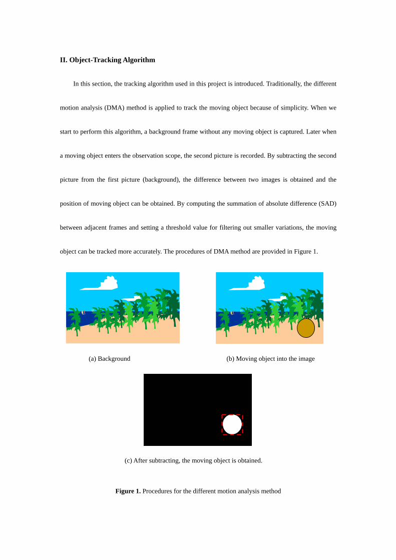
In this section, the tracking algorithm used in this project is introduced. Traditionally, the different

motion analysis (DMA) method is applied to track the moving object because of simplicity. When we

start to perform this algorithm, a background frame without any moving object is captured. Later when

a moving object enters the observation scope, the second picture is recorded. By subtracting the second

picture from the first picture (background), the difference between two images is obtained and the

position of moving object can be obtained. By computing the summation of absolute difference (SAD)

between adjacent frames and setting a threshold value for filtering out smaller variations, the moving

object can be tracked more accurately. The procedures of DMA method are provided in Figure 1.

Figure 1. Procedures for the different motion analysis method

(a) Background (b) Moving object into the image

(c) After subtracting, the moving object is obtained.

However, when the moving object exists in both adjacent frames, the tracking area of moving

object would be overestimated (as shown in Figure.2). In order to overcome this disadvantage of DMA

method, the Block-Matching Algorithm (BMA), in which motion estimation is utilized to adjust the

size of tracking area, is used.

Figure 2. The disadvantage of different motion analysis method

The basic idea of BMA (see Fig. 3) is to divide the current frame in video sequence into

equal-sized small blocks. For each block, we try to find the corresponding block from the search area

of previous frame, which “matches” most closely to the current block. Therefore, this “best-matching”

block from the previous is chosen as the motion source of the current block. The relative position of

these two blocks gives the so-called motion vector (MV), which needs to be computed and transmitted.

When all motion vectors of the blocks in tracking area have been found, the motion vector happened

(a) Background (b) Next image

(c) After subtracting, the tracking area is larger than the moving object size

most frequently is chosen for the correction of tracking area size.

Figure 3. BMA is used to correct the size of tracking area

Typically, the sum of absolute difference (SAD) is selected to measure how closely two blocks

match with each other, because the SAD doesn’t require multiplications; in other words, less

computation time and resources are needed. For the current frame, we denote the intensity of the pixel

with coordinate (I,j) by I(i,j) . For a block of N with coordinate (i,j) , we represent it as ( , )nI i j . We

refer a block of N N× pixels by the coordinate (k,l) of its upper left corner. Then, the SAD between

the block (k,l) of the current frame n, and the block (k+x,l+y) of the previous frame n-1 can be written

as:

( ) ( )1 1

( , ) 10 0

, ,N N

k l n ni j

SAD I k i l j I k x i l y j− −

−= =

= + + − + + + +∑ ∑

The motion vector u(k,l) of the block (k,l) is then given as:

( , ) ( , )( , ) arg min ( , )x y k lu k l SAD x y=

(a) Background (b) Next image

(c)The tracking area size can be corrected by the motion vector

There are several methods used to find out the best matching block. The basic one is the

full-search (FS) method. Assume that the frame size is 320×240 pixels, and each block is 16×16

pixels, there are 20×15 = 300 blocks for each frame. Therefore, total computational amount for the

min MAD with ± 16 search area will be 17× 17× 300=86700 subtractions, 17× 17× 299=86411

additions, and 17×17=289 comparisons. These operations, however, cost a very large computation

complexity and transmission capacity. Hence, many economical searching algorithms have been

developed. Among them the three-step-search (TSS) is very popular due to its speed, regularity in the

search pattern, and the ease in hardware implementation. The TSS algorithm employs a halfway stop

technique to reduce the number of checking points (CPs), thus decreasing the computational

complexity. It is worth noting that such algorithm is useful only for a small motion sequence. It is thus

very likely to make the search trapped at some certain local minimum value.

As a result, in order to compromise the mean square error (MSE) and computational complexity

(speed), the 41SW/BPD algorithm developed by A. C.K.Ng and B. Zeng is applied with some

modifications in our project. This algorithm employs two techniques, namely, (1) 4-to-1 search window

sub-sampling (41SWS) and (2) object boundary pixel decimation (BPD). In the first part of algorithm,

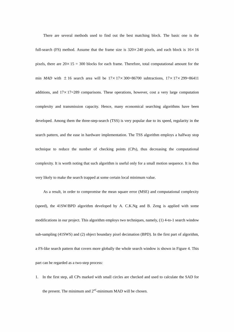
a FS-like search pattern that covers more globally the whole search window is shown in Figure 4. This

part can be regarded as a two-step process:

1. In the first step, all CPs marked with small circles are checked and used to calculate the SAD for

the present. The minimum and 2nd-minimum MAD will be chosen.

2. In the second step, the eight surrounding CPs (marked with small squares) of either one of the two

CPs found in the first step are checked. Among these 18 CPs. The one with the minimum SAD will

be chosen as the ultimate matching block. The vector between the original block and the ultimate

matching block is the motion vector (MV), which can be used to predict the block motion in the

next image.

Figure 4 A FS-like search pattern

For the second part, for searching the object boundary, Ng and Zeng used the so-called object

boundary pixel decimation (BPD). The idea of the BPD method is that the pixels from highly active

areas in spatial domain such as edges will make major contributions to the SAD measurement, so the

most “relevant” or “representing” pixels for doing the block matching should be chosen. Unlike Ng and

Zeng’s method that all objects in the image would be tracked, we assumed only one moving object in

the observation scope in any time.

III. Implementation methodology

We can summarize three steps for implementing our motion-tracking algorithm. The first step is to

capture the images from I/O devices and to transfer each frame from RGB values into corresponding

YUV values. Here we need to use Y (luminance) component as the basic element for computation. As

we know that RGB values are limited from 0 to 255, and the coefficients for computing Y value are

constants. Hence we can optimize the transferring speed by pre-computing all partial values

corresponding to different (R, G, B) values and storing them in a read-only memory (ROM). When a

set of RGB values is received, the corresponding partial values can be read out from the ROM and sent

to adders. The computation cost has changed from three multiplications and two additions to three

memory look-ups and two additions, and actually it is critical for DSP processors.

After gathering all Y values from frames, the SAD values between two adjacent frames are

computed for searching the moving scope of motion object. Each frame can be separated as equal size

blocks, and SAD operation would be performed on each block and the corresponding block in the

adjacent frame. In our project the size of captured frame is 320x240, and the size of block is 16x16.

Therefore each frame would contain 20x15=300 blocks, and then 300 SAD values would be obtained

between two adjacent frames. In this step the operation are the same for each frame, therefore the

parallel processing optimization can also be used as much as possible in implementation.

CapturingBackground Image

Capturing Images

Subtraction of Image A and Image B

If SAD is larger than the Threshold ?

NoSubtraction of

Image B and Background Image

If SAD is larger than the Threshold ?

YesPosition these blocks and set

A <- B

No

Block Relation Test

YesNo

Position these blocks and set

A <- BCounter

Counts <=10 Counts>10

A<-B Background<-B

Yes

Position the blocks

41SWSAlgorithm

Motion Vectorand position

blocks

A<-B

Figure 5. The flow graph of our motion-tracking algorithm

In order to compensate for the error range of tracking area, motion estimation needs to be

performed. The motion vector of each block inside the imprecise tracking area could be found by

computing MAD from SAD values to all blocks inside the search area of adjacent frame. However, it

would cost lots of resources to implement this step if full search is used. At first we replace the full

search method with a novel full-search like sub-sampling algorithm 41SWS/BPD, and then we focus

on the motion estimation computation on the blocks with largest SAD values to further speed up the

execution of algorithm without significant loss of performance.

IV. Implementation by Borland C++ Builder

In order to realize the real-time object tracking algorithm on embedded system, we first simulate

the algorithm on Borland C++ Builder and try to optimize it. There are several challenges we have to

overcome and we will discuss them in the following passage.

Grab Image From Webcam

First of all, we need to grab image from the webcam as fast as possible. However, our webcam only

support USB 1.1 that ideally can only provide 11 Mbytes per second. But the actual speed is far less

than the ideal one because of the package overhead, propagation delay, handshaking between host

and slave etc. The actual image transmitting speed we measured is about seven 320x240 frames per

second.

Implement tracking algorithm

The original tracking algorithm is pretty simple. It firstly subtracts two frames and calculates the

SAD value for each block. If the SAD value bigger than the threshold value, the block will be

recorded as the motion block. The problems of this algorithm we have mentioned in the previous

section. In order to have more precise tracking algorithm, we try to find three blocks that have

biggest SAD value. Then we use 41SWS/BPD to find out the motion vector of each block. If two of

these three motion vectors are the same, we will see it as a valid motion vector and use it to fix the

tracking area. The result shows that it can actually provide more precise tracking area.

Background changing problem

The changing of background will also have a big influence of the object tracking algorithm.

Therefore, we provide a background update algorithm to minimum the influence. The background

update algorithm will active only if there is no tracking object in the frame. When there is no

tracking object, the background update algorithm will update the background for every 10 frames. If

the motion blocks in a frame is bigger than 5, the algorithm will be terminated and go into tracking

mode. By this mechanism, the tracking algorithm can tolerant slightly background changing such as

the light etc.

Build up a human interface

In order to show up the tracking result on the screen, we try to build up a simple human interface.

The detail of the human interface is shown below (Fig. 6).

Figure 6. The human interface window

1

2

3

4

5

Table 1. Block descriptions

Block Num Description

1 Show up the original image grabbed from the webcam.

2

Show up the tracking result of the image. The blue frame is the object

tracking area. The three small squares are the blocks having the

maximum SAD value. We calculate the motion vectors of these three

blocks to provide precise tracking area.

3

The control panel. If want to run the tracking algorithm at ET44M210,

user must select the check box “Use ET44M210” and push the

“Connect” button to connect to hardware. Note that the ET44M210

should connect to PC through USB first or the program will be

terminated.

4 Message panel. Provide tracking information.

5 Speed panel. Show up the average process speed. The unit is frames

per second.

V. Implementation by ET44M210

The ET44M210 is a 8-bit architecture microprocessor. The biggest advantage of ET44M210 is the

low cost. It only needs less than 1 dollar for a single chip. Comparing to TI DSP microprocessor, it

does not support too many powerful instructions and can only run at 48MHz, but only cost 1/20.

Therefore, it is suitable for embedded real-time object image tracking system.

The ideal system is shown on figure 7. We firstly use a CMOS camera module to grab image.

ET44M210 will take charge for setup and control the camera module, and read image data form it.

Once ET44M210 get the image, it will start to run the tracking algorithm and find out the motion of

object. Finally, it will use the motion vector to control the step motor or send the tracking result to

central controller through antenna. In reality, we do not have the camera module and the step motor.

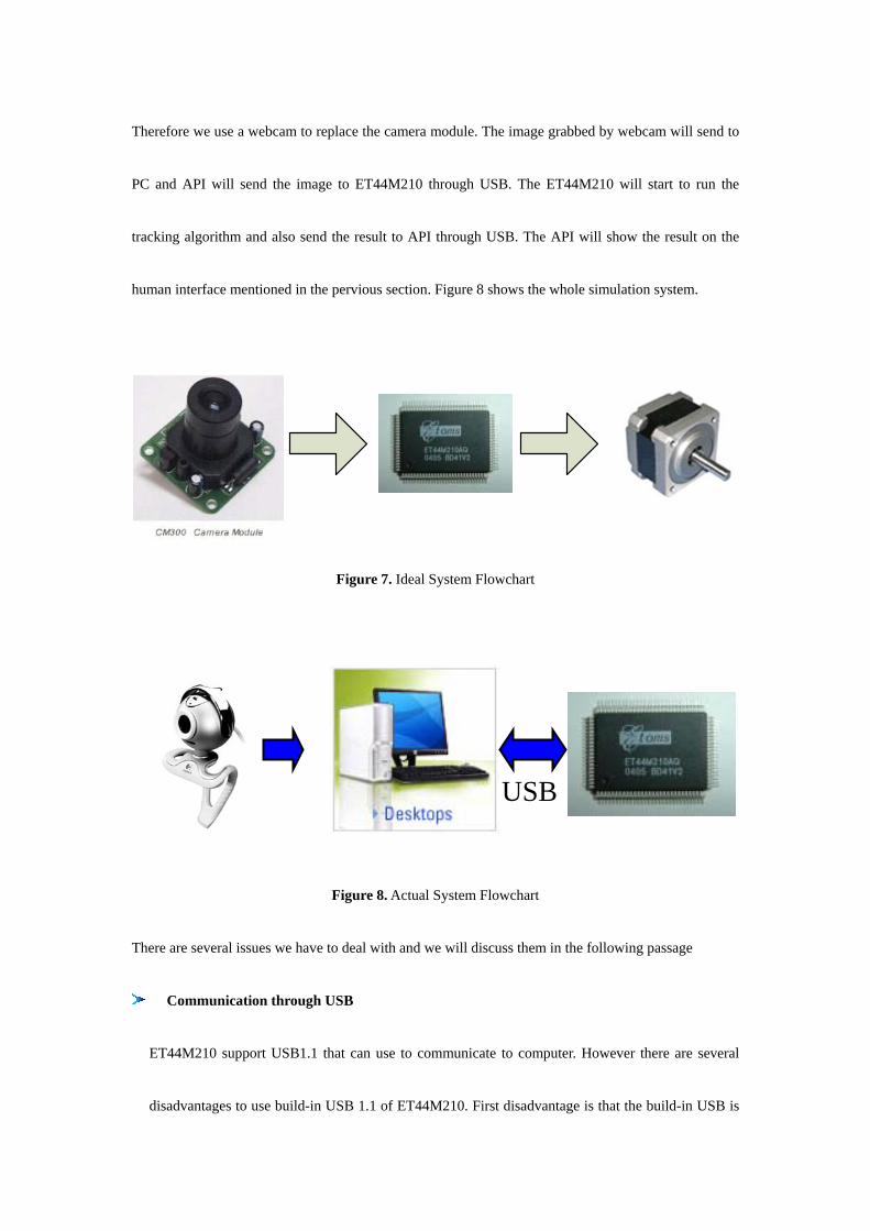
Therefore we use a webcam to replace the camera module. The image grabbed by webcam will send to

PC and API will send the image to ET44M210 through USB. The ET44M210 will start to run the

tracking algorithm and also send the result to API through USB. The API will show the result on the

human interface mentioned in the pervious section. Figure 8 shows the whole simulation system.

Figure 7. Ideal System Flowchart

Figure 8. Actual System Flowchart

There are several issues we have to deal with and we will discuss them in the following passage

Communication through USB

ET44M210 support USB1.1 that can use to communicate to computer. However there are several

disadvantages to use build-in USB 1.1 of ET44M210. First disadvantage is that the build-in USB is

USB

not a separate hardware structure that we must spend lots of instructions to control the USB. Second

is that the standard of USB 1.1 support “bulk transmission mode” for up to 512 bytes per package.

Nevertheless, the build-in USB only support 64 bytes per package. It will create lots of package

overhead and degrade the transmission performance. The influence of USB will discuss later.

Create Y from RGB

Now we will talk about the implement methodology of the tracking algorithm. First part is that we

must calculate the Y value base on RGB. The formula of the conversion is Y = 0.299R + 0.587G +

0.114B. As you can see, it will need three multiples and two additions to get the result. As mention

before, the value of RGB is 0 to 255 and we will build up three 255 entries tables on ROM. Hence,

we can reduce the computation complexity to 3 look-up table operations and two additions. The

problem is that how many bits we should use to save a single data? In order to find out the answer,

we write a small program to simulate the results. Base on the results shown on Table 2, we find that

use 8-bit resolution will be enough since the average error is 1.492 that far less than the motion

threshold.

Table 2 Simulation results

Resolution Average error Max error

8 bits 1.492 2.981

16 bits 0.498 1.001

Calculate SAD for all blocks

The internal memory of ET44M210 is sufficient to save two blocks at a same time. Therefore, we

first load two blocks to ET44M210 and subtract two blocks to get the SAD value. The ET44M210

can support up to 4 Mbytes external memory, and two different frames should store in the external

memory. The problem is that we do not have an external memory module. To solve this problem, we

create a 4 Mbytes memory space on PC and ET44M210 can access the memory through USB. Of

course, the speed to access external memory through USB is far less than direct access the external

memory; it will also cause performance degradation.

Find out motion vectors

The policy to find motion vectors is similar to calculate SAD. We will load the base block to

ET44M210 first and replace the comparison block to find out the minimum SAD.

Evaluation

Since the transmission speed of USB 1.1 seems to be the bottleneck of the whole system, we try to

calculate the instructions consumed by core tracking algorithm and neglect the influence of USB. To

find out the total instructions consumed by core tracking algorithm, we use a separate timer structure

supported by ET44M210 that can calculate the total cycles for the algorithm. The results are shown

on Table 3. Form the table, we can find that the total instructions consumed by core tracking

algorithm is about 4.3 M. If we run the ET44M210 at full speed mode (48 MHz), we can achieve

handle 11 frames / second. But the maximum frames we can handle in the simulation system are

about 0.9 frames per second. One reason is that the ET44M210 can only run at 24 MHz when using

USB system (need to synchronize with USB clock). Another reason is that we need to spend lots of

instruction to handle USB transmission and propagation delay and handshaking will also influence

the performance.

Table 3 Simulation result

Type Inst / frame

Grab image 460800

Convert Y 3234600

Calculate SAD 161100

Find MVs 491355

Summation 4347855

frames/sec 11.04

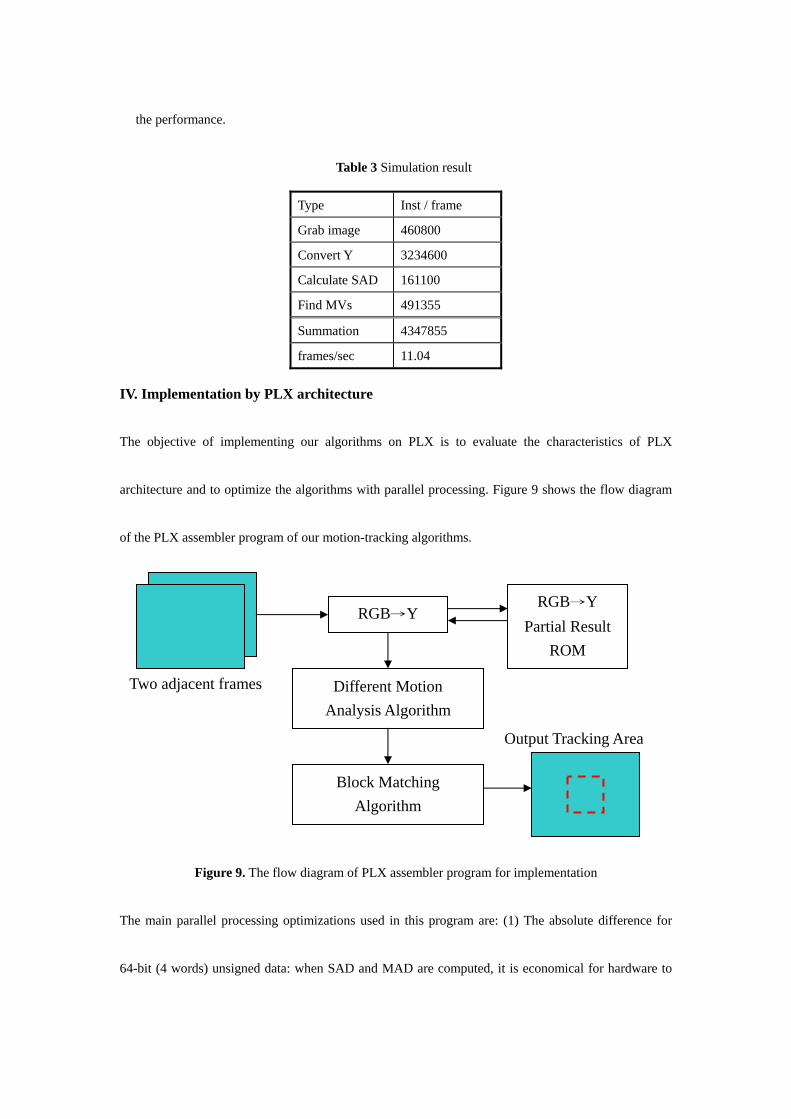
IV. Implementation by PLX architecture

The objective of implementing our algorithms on PLX is to evaluate the characteristics of PLX

architecture and to optimize the algorithms with parallel processing. Figure 9 shows the flow diagram

of the PLX assembler program of our motion-tracking algorithms.

Figure 9. The flow diagram of PLX assembler program for implementation

The main parallel processing optimizations used in this program are: (1) The absolute difference for

64-bit (4 words) unsigned data: when SAD and MAD are computed, it is economical for hardware to

Two adjacent frames

RGB→Y RGB→Y

Partial Result ROM

Different Motion Analysis Algorithm

Block Matching Algorithm

Output Tracking Area

perform the same operation to multiple data. Here we integrate four Y values from different pixels in

one block into one register to decrease the processing time of absolute difference. (2) The alignment of

four different load/store data: when load or store data from/to memory, there may be some problems

without the data alignment because PLX only can accept the address that can be divide by four. It is

also the case for several commercial DSP processors. Therefore when we load RGB values from

memory or store it two the LCD address (plot it on the LCD screen), we integrate four adjacent RGB

values into one register. In this way the processing speed can be improved and the alignment problem

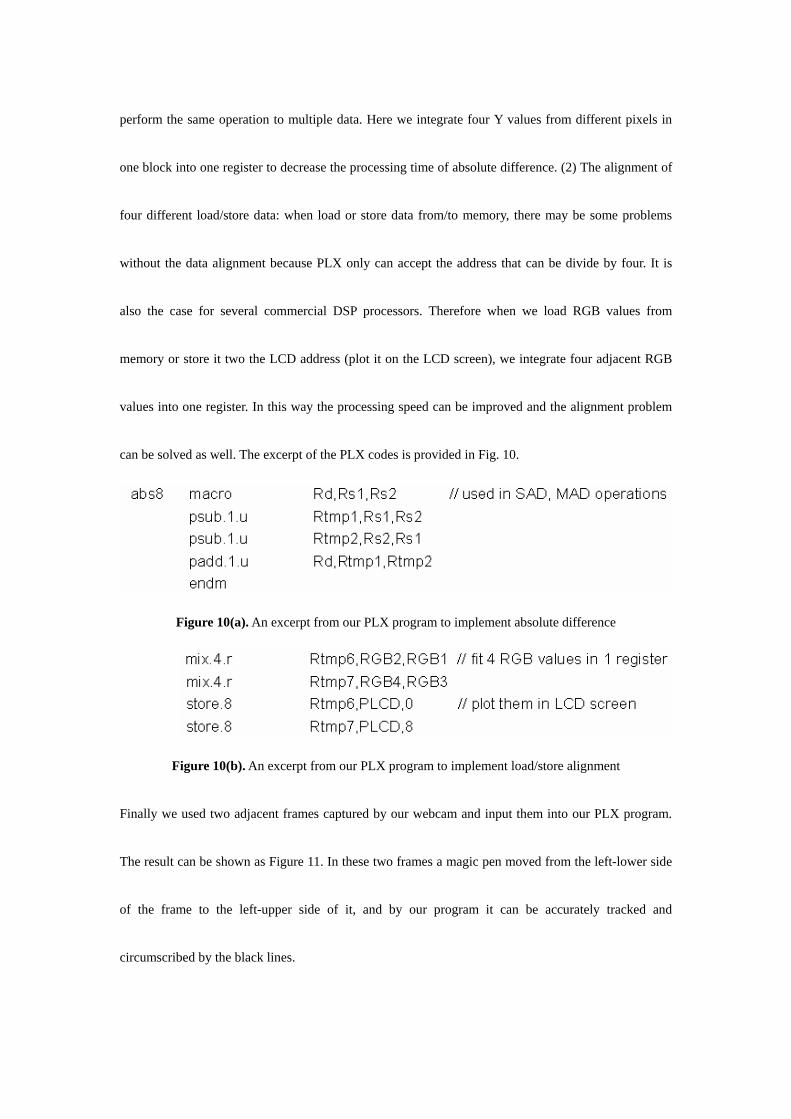
can be solved as well. The excerpt of the PLX codes is provided in Fig. 10.

Figure 10(a). An excerpt from our PLX program to implement absolute difference

Figure 10(b). An excerpt from our PLX program to implement load/store alignment

Finally we used two adjacent frames captured by our webcam and input them into our PLX program.

The result can be shown as Figure 11. In these two frames a magic pen moved from the left-lower side

of the frame to the left-upper side of it, and by our program it can be accurately tracked and

circumscribed by the black lines.

Figure 11. The example of motion-tracking algorithm in PLX implementation

IIV. Conclusion

In this project, the real-time object image algorithms – Different Motion Analysis with

Block-Matching Algorithm have been introduced and implemented on ET44M210 microprocessor on

and PLX architecture. For ET44M210, the maximum frames we can handle in the simulation system

are about 0.9 frames per second because of transmission speed limit of USB interface, but the moving

object with moderate velocity can still be tracked. In PLX simulation, the optimizations of the

algorithms with parallel processing have been realized and some basic and correct tracking results can

be achieved. The source codes are provided in https://mywebspace.wisc.edu/twu3/web/734sp06.html.

With limited hardware resources, some performance trade-offs and system optimizations are still

necessary for applying motion tracking algorithms on commercial DSP processors. In some recent

literatures deformable active contour algorithm has been proposed as a high-speed solution for medical

image tracking and implemented on TI DSP chips, and in the future it needs to be optimized in

different commercial DSP processors.

IIIV. Reference

C.K. Ng, and B. Zeng, “A new fast motion estimation algorithm based on search window sub-sampling

and object boundary pixel block matching,” Proc. ICIP ’98, vol.3, pp.605-608, Oct. 1998.

S.A. El-Azim, I, Ismail, and H.A. El-Latiff, “An efficient object tracking technique using

block-matching algorithm,” Proc. Of the Nineteen National, Radio Science Conf., pp.427-433,2002.

Y.L., Chan and W.C. Siu, “New adaptive pixel decimation for block motion vector estimation”, IEEE

Trans. Circuit and Systems fro Video Tech., vol. 4, no 4, Aug. 1994.

R. Li, B.Zeng an dM. Liou, “A new three step search algorithm for block motion estimation”, IEEE

Trans. Circuit and Systems fro Video Tech. vol. 6. no 1, Aug. 1994.

J. Zapata, and R. Ruiz, “Solution based on a DSP processor for high-speed processing and motion

tracking of endocardial wall”, Proc. SPIE., vol. 4491, p. 346-357, Nov. 2001.