real-time management of transportation disruptions in forestry · real-time management of...

Real-Time Management of Transportation Disruptions in Forestry Amine Amrouss Nizar El Hachemi Michel Gendreau Bernard Gendron March 2016 CIRRELT-2016-13

Real-Time Management of Transportation Disruptions in Forestry

Amine Amrouss1,2,*, Nizar El Hachemi1,3, Michel Gendreau1,4, Bernard Gendron1,2

1 Interuniversity Research Centre on Enterprise Networks, Logistics and Transportation (CIRRELT) 2 Department of Computer Science and Operations Research, Université de Montréal, P.O. Box

6128, Station Centre-Ville, Montréal, Canada H3C 3J7 3 Université Mohammed V de Rabat, École Mohammadia d’Ingénieurs, Avenue Ibnsina B.P. 765,

Agdal, Rabat, Maroc 4 Department of Mathematics and Industrial Engineering, Polytechnique Montréal, P.O. Box 6079,

Station Centre-Ville, Montréal, Canada H3C 3A7

Abstract. In this paper, we present a mathematical programming model based on a time-

space network representation for solving real-time transportation problems in forestry. We

cover a wide range of unforeseen events that may disrupt the planned transportation

operations (e.g., delays, changes in the demand and changes in the topology of the

transportation network). Although each of these events has different impacts on the initial

transportation plan, one key characteristic of the proposed model is that it remains valid

for dealing with all the unforeseen events, regardless of their nature. Indeed, the impacts

of such events are reflected in a time-space network and in the input parameters rather

than in the model itself. The empirical evaluation of the proposed approach is based on

data provided by Canadian forestry companies and tested under generated disruption

scenarios. The test sets have been successfully solved to optimality in very short

computational times and demonstrate the potential improvement of transportation

operations incurred by this approach.

Keywords. Real-time, transportation, forestry, mathematical programming.

Acknowledgements. The authors would like to thank the Natural Sciences and

Engineering Research Council of Canada (NSERC) Strategic Network on Value Chain

Optimization (VCO) for their financial support. In addition, we wish to thank FPInnovations

for their valuable collaboration.

Results and views expressed in this publication are the sole responsibility of the authors and do not necessarily reflect those of CIRRELT.

Les résultats et opinions contenus dans cette publication ne reflètent pas nécessairement la position du CIRRELT et n'engagent pas sa responsabilité. _____________________________ * Corresponding author: [email protected]

Dépôt légal – Bibliothèque et Archives nationales du Québec Bibliothèque et Archives Canada, 2016

© Amrouss,El Hachemi, Gendreau, Gendron and CIRRELT, 2016

1. Introduction

Optimization models and operations research (OR) methods have been used

in the forest industry since the 1960s [1]. Recent reviews on how these mod-

els and methods are used to solve planning problems in forestry can be found

in [2, 3]. These planning problems cover a wide range of activities such as

sylviculture, harvesting, road building, production and transportation, which

present to this day several challenges to OR practitioners [4, 5], as the forest

industry attempts to improve its competitiveness and reduce its environmental

impact. In particular, improving transportation planning in forestry has been

the object of recent research of highly practical relevance, since transportation

costs are estimated at more than one-third of wood procurement costs [5]. Min-

imizing transportation costs therefore represents a key element to improve the

competitiveness of forest companies.

Recently, a number of OR models and methods have been developed to

solve the log-truck scheduling problem (LTSP) [6, 7, 8, 9, 10], which consists

in deriving schedules for trucks to transport different wood products between

forest sites and wood mills. In addition, several decision support systems, such

as the ASICAM project in Chile [10] and the EPO project in Finland [11],

were developed to ease transportation planning. A review of transportation

planning systems in the forest industry and the contribution of OR in their

development can be found in [12]. Note that few decision support systems are

available to forest companies (compared to other industrial sectors [13]), as

many forest companies still rely on experienced dispatchers to manually derive

their transportation plans.

Whether the transportation plans are obtained through an optimization

method or manually, their implementation in practice is vulnerable to unfore-

seen events. For example, in Canada, spring thawing soils and summer rains

degrade the forest roads condition and prevent the trucks from accomplishing

their trips within the planned time. The late arrival of these trucks may also

create queues for loading and unloading operations. In this case, the disrup-


CIRRELT-2016-13 1

tion consequences may stream through the whole supply chain and many trips

could become infeasible. There is then a need to re-optimize the transportation

plan as early as possible to minimize the impact of such disruptions. Real-time

rescheduling of log-trucks has not been subject to much attention in the liter-

ature, in spite of the growing body of literature on similar problems in other

industrial sectors, with the advent of intelligent transportation systems [14].

To the best of our knowledge, CADIS (for Computer Aided Dispatch) is the

only documented decision support system for real-time dispatching in forestry

[15]. The authors reported very few details about this system because of non-

disclosure agreements with the New Zealand company that used it. The system

produced encouraging results [16], although it was used only for a short period,

as the company ceased its activities because of financial issues. Other commer-

cial decision support systems [12] may include real-time dispatching modules,

but they are generally manually managed. The recent work [5] defines real-time

transportation management as one of 33 open problems in the forest industry

for OR practitioners.

The most frequent source of uncertainty irelated to transportation planning

problems in other industrial sectors is the arrival of new requests (e.g., new

customers or change in the demand) [17, 18]. In forest transportation planning

problems, one must deal with unforeseen events of a different nature such as

changes in the topology of the transportation network (e.g., road closure). In

this paper, we propose a mathematical programming model that remains valid

for every unforeseen event that may occur during forest transportation oper-

ations, regardless of its nature. The model is based on a time-space network

representation of the forest supply chain where the impacts of the unforeseen

events are represented.

The remainder of this paper is organized as follows. Section 2 describes the

problem, starting with a generic description of the LTSP. Section 3 presents

the proposed approach to re-optimize the transportation plan in real-time in

response to an unforeseen event. The description of the test sets and the results

of our approach are presented in Section 4. Section 5 concludes this work.


2 CIRRELT-2016-13

2. Problem description

We begin this section with a generic description of the LTSP, whose solution

produces a transportation plan that consists of a sequence of empty and loaded

trips in addition to loading and unloading operations. Note that our approach

remains valid whether such a plan is derived manually or by using optimization

methods, but the LTSP provides a conceptual framework for the subsequent

development of our model for real-time rescheduling of log-trucks.

We assume a homogeneous fleet of trucks. Each truck is associated with a

base, usually a wood mill, where it must begin and end its shift. The planner

must assign a route to each truck over a planning horizon of one week. A

route is composed of a set of trips in addition to waiting, loading and unloading

operations. We define as R, V , M , and F the sets of routes, trucks, mills and

forest sites, respectively. Rv is the subset of routes linked to truck v ∈ V .

Each route r ∈ R has a cost cr. This cost includes productive (loaded trips,

loading and unloading) and unproductive activities (empty trips and waiting).

The LTSP aims at minimizing the total cost while satisfying the demand Dm

at each mill m ∈ M given a certain amount of available wood products Sf at

each forest site f ∈ F . The problem can be formulated as follows [3]:

Min∑r∈R

cryr (1)∑r∈R

bmryr = Dm, ∀m ∈M (2)∑r∈R

afryr ≤ Sf , ∀f ∈ F (3)∑r∈Rv

yr = 1, ∀v ∈ V (4)

yr ∈ {0, 1} ∀r ∈ R (5)

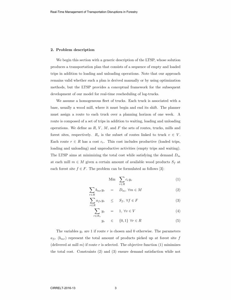
The variables yr are 1 if route r is chosen and 0 otherwise. The parameters

afr (bmr) represent the total amount of products picked up at forest site f

(delivered at mill m) if route r is selected. The objective function (1) minimizes

the total cost. Constraints (2) and (3) ensure demand satisfaction while not


CIRRELT-2016-13 3

exceeding the supply. Constraints (4) ensure that at each truck is assigned a

route.

Note that the transportation cost includes a fixed cost for using a truck and

a variable cost proportional to the distance that depends on whether the truck

is empty or loaded. The trucks have to travel empty from the mills to the forest

sites. Thus, a truck that operates only trips between the same mill and the same

forest site loses half of its transportation capacity. Instead, once at a mill, one

must try to allocate the wood products from the closest forest sites to the mills

in the opposite direction. This is known in the literature as backhauling and

we refer the interested reader to [19] for more details about decision support

systems using backhauling in the forest industry.

Loading and unloading operations are performed by loaders at forest sites

and mills. These loaders are usually operated only for a specific period of the

day. Moreover, the number of loaders available at a mill or a forest site may

vary during the day. To avoid creating queues at the loaders and thus reduce

the cost of unproductive activities, another objective that must be met by the

dispatcher is the synchronization of the trucks with the loaders given accurate

information about the available loaders. These constraints appear in the recent

works on the LTSP [6, 9] and are considered in our work.

In the context of real-time rescheduling of log-trucks, we assume that truck

drivers receive one trip at a time, the dispatcher waiting for each truck driver to

finish its current trip before revealing its next destination. This mode of trans-

portation planning management gives more flexibility to re-optimize the routes,

since it avoids drivers resistance to change. While re-optimizing the transporta-

tion plans following the occurrence of an unforeseen event, the dispatcher must

avoid diverting a truck from its destination unless the unforeseen event pre-

vents the completion of the current trip. This improves the consistency of the

proposed schedules and facilitates their real-life implementation. Moreover, in

a real-time context, the amount of time available to the dispatcher to derive

alternative transportations plans is limited.

The nature of the unforeseen events that arise in the forest industry is dis-


4 CIRRELT-2016-13

tinct from what can be found in the literature on similar problems found in

other industrial sectors. We have drawn up a list of the most frequent unfore-

seen events. The list includes unforeseen events that are likely to appear at

the forest sites, those involving trucks and road networks, and the events that

occur at the mills. To develop effective recourse strategies when facing such

events, one must focus on the impacts they have on the transportation network

rather than on the events themselves. The next section describes the proposed

approach to implement these recourse strategies.

3. Proposed approach

Our approach to real-time rescheduling log-trucks is built on a time-space

network representation, which is used in the definition of our mathematical

programming model. The time-space network represents the evolution of the

forest supply chain over time. This representation varies depending on the

nature of the unforeseen events that are revealed over time. The space and

time dimensions of the network allow to track the trucks in real-time and to

capture the impacts of the unforeseen events on the transportation network

(e.g., by removing the arcs that become inaccessible). The distances between

two locations in the transportation network are expressed as a time measure.

This helps to capture the impact of some unforeseen events. In the case of a

road degradation or a traffic jam, for example, the trip duration may become

longer, while the geographical distance remains the same. The mathematical

programming model takes this time-space network as an input and is solved

using a commercial solver.

3.1. Time-space network

When an unforeseen event is revealed, one must collect real-time information

about the state of the transportation network elements. We refer to the state of

a truck, for example, as the information about its position, its destination and

the product it is transporting if it is loaded. Moreover, if the truck is directly


CIRRELT-2016-13 5

Figure 1: Time-space network

impacted by the unforeseen event as in the case of a truck breakdown, we as-

sume that we have additional information about the estimated characteristics of

the corresponding event, such as an estimate of the truck repair duration. The

collection and validation of these estimates is beyond the scope of this work, but

the current development of onboard computers, geo-location and communica-

tion technologies, in addition to the development of big data algorithms, make

the collection of good quality estimates of the disruptions characteristics more

affordable and easier.

The state of the transportation network can be seen as an instant picture of

this network that we represent as a time-space network. The space dimension

of the network contains the set of wood mills and forest sites in addition to their

linking roads. For the time dimension of the network, we divide the planning

horizon into a set of intervals. The necessary time for loading and unloading

operations is approximately equal and the driven distances are quite large in

the context we consider in this paper. Therefore, we use the loading duration


6 CIRRELT-2016-13

as a time-step for discretizing the planning horizon. The time-space network

representation (Figure 1) contains four types of vertices :

• A source vertex for each truck representing its current location (or its base

if it has not yet started its shift) when the unforeseen event is revealed.

These individual truck vertices are different from what can be found in

a conventional time-space network. We need to introduce them to track

the truck positions in real-time. Note also that the trucks that finish their

shift before the occurrence of the disruption are not represented in the

network.

• A sink vertex for each truck. It corresponds to its base and represents the

shift end for the truck.

• Forest site vertices. Each vertex is replicated for each time interval of the

discretized planning horizon. This allows to capture real-time information

about the forest sites. This includes the current supply of each product

and the number of loaders available at the correspondent interval. These

vertices are duplicated to represent whether the truck is full or empty.

• Mill vertices. They are similarly replicated. The vertex state contains

information about the current demand for each product and the number

of loaders available at the corresponding interval.

The replication of the vertices is done horizontally in Figure 1. Each pair

of lines represents either a mill or a forest site evolving over time. For reasons

of clarity, only a subset of the arcs is represented in Figure 1 and their length

does not represent the real distances. The arcs kept for the first truck give an

example of a small sequence of trips. There are seven types of capacitated arcs

in the time-space network:

• Start arcs connecting source vertices to empty forest site vertices, if the

corresponding truck is empty, and to full mill vertices, otherwise. Their

capacity is one truck.


CIRRELT-2016-13 7

• End arcs connecting empty mill vertices that correspond to a truck base

to this truck sink vertex. Their capacity is one truck.

• Loaded driven arcs connecting a full forest site vertex to a full mill vertex

demanding at least one of the available products at this forest site. Their

capacity is equal to the number of available trucks.

• Empty driven arcs connecting an empty mill vertex to an empty forest site

vertex supplying at least one requested product. Their capacity is equal

to the number of available trucks.

• Waiting arcs connecting two successive mill vertices. Note that, as the

number of mills is usually smaller than the number of forest sites and to

reduce the symmetry, we prefer that the trucks wait at mills instead of at

forest sites. Their capacity is equal to the number of available trucks.

• Loading arcs connecting two successive empty and full forest site vertices.

Their capacity is equal to the number of available loaders.

• Unloading arcs connecting two successive full and empty mill vertices.

Their capacity is equal to the number of available loaders.

It should be noted that the length of the arcs represents the duration of the

corresponding operation. Therefore, these arcs exist only between vertices at

intervals separated by at least this duration. Moreover, the vertices and arcs

constituting this time-space network vary over time and depend on the nature

of the revealed unforeseen events. We describe how these transformations are

done in the following subsection.

3.2. Dealing with disruptions

At the occurrence of an unforeseen event, we first collect the necessary in-

formation about the trips that were executed before the disruption in order to

update the remaining demand and the number of trucks still in operation. We

also collect the relevant information about the trucks, their positions and if they


8 CIRRELT-2016-13

are loaded or empty. Having this information in addition to the estimates of

the unforeseen event impacts, a new time-space network is produced. All the

vertices and arcs that start before the occurrence of the event are removed from

the initial time-space network. One exception is the truck start vertices. Out-

going arcs from these start vertices are updated according to the nature of the

unforeseen event and to the corresponding truck positions.

The recourse strategies when an unforeseen event is revealed depend on its

impact on the transportation network rather than on the event itself. Different

unforeseen events can have the same impact on the transportation network. For

example, in the case of the presence of a single loader at a forest site or at a

mill, the breakdown of this loader can be seen as the corresponding site closure,

assuming that the loaders are not allowed to move between different sites and

that the trucks do not include onboard loaders. The following describes the

disruptions categories based on their impact on the network, in addition to the

corresponding recourse strategies.

Closures

This category contains the closures of forest sites, wood mills and roads.

Also, there is generally one single forest road to access a forest site in contrast

with urban context where the same point may be reached by different paths.

Therefore, the closure of such road can also be considered as a forest site closure.

A mill closure means that no product can be delivered to this mill during the

closure. This can be caused, for example, by a decrease in the storage capacity

or by the breakdown of the loader associated with this mill.

In the event of such disruptions at a mill or at a forest site, we remove the

loading or unloading arcs at the corresponding vertices in addition to outgoing

driven arcs for all time intervals that lie within the estimated duration of the

disruption. We keep the waiting arcs at the mills. For trucks planned to ar-

rive at the closed vertices before the operations start back, their start vertices

are connected to the other mills or forest sites depending on whether they are

loaded or not. The remaining truck start vertices are connected to their current


CIRRELT-2016-13 9

destination at the time the disruption is revealed. The rest of the network is

unchanged. If the disruption occurs on a road linking a mill to a forest site, we

remove the corresponding arcs in the network for all the time intervals that lie

within the closure duration.

Delays

Delays can be caused by a variety of unforeseen events. This includes bad

weather conditions (poor visibility, thawing soils, heavy rains), degradation of

forest roads, traffic jams, opening of hunting or fishing season and so on. Delays

can be observed at a single truck level. This is the case, for example, when the

truck is undergoing some mechanical issues and thus slowing down. In contrast,

when a forest road is damaged, for instance, all the trucks taking this road will

be impacted.

When a truck is delayed, we link its start vertex to its current destination

vertex but at an interval that takes into account both the remaining distance

and the estimation of the delay. For delays observed between two vertices, we

move the arcs to take into account the delay estimation. We do so for all the

arcs that lie within the estimation of the duration necessary to return to normal

operations.

A truck breakdown can also be seen as a delayed truck. We assume that we

have an estimate of the necessary time to repair this truck. If the repair time

does not exceed the planning horizon, the arrival time of the truck to its next

destination is delayed by the repair duration. Otherwise, we just remove the

truck from the network.

Demand and supply variations

Mill breakdowns may lead to a decrease in its storage capacity. The demand

of some products must therefore be adjusted downwards. Also, we may have an

increase in the demand for some products. If the mill is not already connected to

forest sites where the product is available, we add empty and loaded driven arcs

between the mill and these forest sites. We also adjust the demand parameter


10 CIRRELT-2016-13

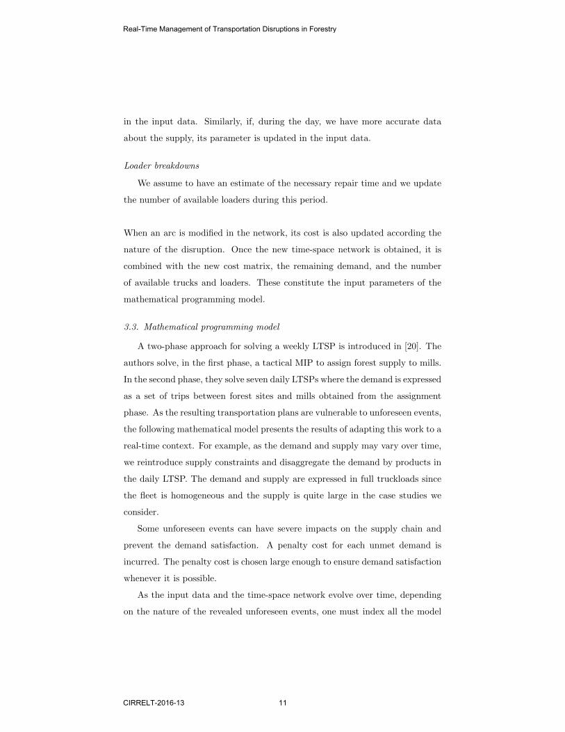
in the input data. Similarly, if, during the day, we have more accurate data

about the supply, its parameter is updated in the input data.

Loader breakdowns

We assume to have an estimate of the necessary repair time and we update

the number of available loaders during this period.

When an arc is modified in the network, its cost is also updated according the

nature of the disruption. Once the new time-space network is obtained, it is

combined with the new cost matrix, the remaining demand, and the number

of available trucks and loaders. These constitute the input parameters of the

mathematical programming model.

3.3. Mathematical programming model

A two-phase approach for solving a weekly LTSP is introduced in [20]. The

authors solve, in the first phase, a tactical MIP to assign forest supply to mills.

In the second phase, they solve seven daily LTSPs where the demand is expressed

as a set of trips between forest sites and mills obtained from the assignment

phase. As the resulting transportation plans are vulnerable to unforeseen events,

the following mathematical model presents the results of adapting this work to a

real-time context. For example, as the demand and supply may vary over time,

we reintroduce supply constraints and disaggregate the demand by products in

the daily LTSP. The demand and supply are expressed in full truckloads since

the fleet is homogeneous and the supply is quite large in the case studies we

consider.

Some unforeseen events can have severe impacts on the supply chain and

prevent the demand satisfaction. A penalty cost for each unmet demand is

incurred. The penalty cost is chosen large enough to ensure demand satisfaction

whenever it is possible.

As the input data and the time-space network evolve over time, depending

on the nature of the revealed unforeseen events, one must index all the model


CIRRELT-2016-13 11

parameters and variables by the event category and by their occurrence time.

However, for the sake of clarity and ease of reading, we omit these indices.

Hereafter, we list the parameters and the variables of the model, and then

introduce the model itself.

Parameters

F : set of forest sites,

M : set of mills,

V : set of trucks,

P : set of wood products,

I : set of time intervals,

N : set of vertices,

A : set of arcs,

A+(n) : set of outgoing arcs from vertex n,

A−(n) : set of incoming arcs into vertex n,

Aloadedfmp : set of loaded driven arcs from forest site f to mill m transporting wood

product p,

AWLE : set of waiting, loaded and empty driven arcs,

Startv : start vertex for truck v,

Endv : end vertex for truck v,

AUmi : unloading arc at mill m at time interval i,

ALfi : loading arc at forest site f at time interval i,

ca : cost associated with arc a,

c : penalty cost of unmet demand,

ua : capacity of arc a,

dmp : demand of product p at mill m,

sfp : supply of product p at forest site f ,

lmi : number of available loaders at mill m at time interval i,

lfi : number of available loaders at forest site f at time interval i.


12 CIRRELT-2016-13

Variables

xa : number of trucks that follow arc a,

δmp : unmet demand of product p at mill m.

Model

Min∑a∈A

caxa +∑m∈M

∑p∈P

cδmp (6)

∑a∈A+(Startv)

xa =∑

a∈A−(Endv)

xa, ∀v ∈ V (7)

∑a∈A+(n)

xa =∑

a∈A−(n)

xa, ∀n ∈ N\ ∪v∈V {(Startv, Endv)} (8)

∑f∈F

∑a∈Aloaded

fmp

xa + δmp = dmp, ∀m ∈M,∀p ∈ P (9)

∑m∈M

∑a∈Aloaded

fmp

xa ≤ sfp, ∀f ∈ F,∀p ∈ P (10)

xa ∈ {0, 1} , ∀a ∈ A+(Startv) ∪A−(Endv) (11)

xa ∈ {0, . . . , lmi} , ∀m ∈M, ∀i ∈ I, ∀a ∈ AUmi (12)

xa ∈ {0, . . . , lfi} , ∀f ∈ F,∀i ∈ I, ∀a ∈ ALfi (13)

xa ∈ {0, . . . , ua} , ∀a ∈ AWLE (14)

δmp ∈ {0, . . . , dmp} , ∀m ∈M, ∀p ∈ P (15)

The objective function (6) minimizes the total cost, including waiting, load-

ing and unloading, and loaded and empty driven trips. The total cost includes

also the penalty costs of the unmet demand. Constraints (7) ensure that every

used truck goes back to its base. Constraints (8) are flow conservation con-

straints for each mill and forest site vertex. Constraints (9) and (10) guarantee

the satisfaction of the remaining demand while not exceeding the supply. Con-

straints (11) ensure the unicity of the capacity of start and end arcs. Constraints

(12) and (13) ensure that each loader only serves one truck at a time. Con-

straints (14) limit the capacity of waiting, loaded and empty driven arcs to the

number of available trucks. Finally, constraints (15) ensure the non-negativity

of the unmet demand and limits its value to the actual demand.


CIRRELT-2016-13 13

We assume that we have a weekly transportation plan as the starting point.

The transportation operations follow this schedule until an unforeseen event

is revealed. The time-space network and the input parameters are updated

according the nature of the unforeseen event, then we solve the model for the

current day. The new transportation plan is used until another unforeseen event

is revealed and the same operation is repeated until the end of the planning

horizon.

4. Computational results

FPInnovations, a non-profit forest research centre dedicated to the improve-

ment of the Canadian forest industry through innovation, provided us with six

case studies from Canadian forest companies. All these case studies represent

weekly planning problems. Moreover, we developed a disruptions generator that

produces several “weeks” of unforeseen events. A week of unforeseen events is

a set of disruptions scattered over one week. The goal is to assess the proposed

approach performance on different forest supply chain configurations under dif-

ferent disruption scenarios. The main performance indicators considered in this

paper are demand satisfaction, transportation cost and computational time.

4.1. Unforeseen events

Unforeseen events have different impacts on the transportation network. For

testing purposes, these events and their impacts are randomly generated. We

developed a discrete-event model that produces a succession of events that hap-

pen at different discrete times. Note that different events are allowed to happen

at the same time. The aim of this simulation is to generate unforeseen events

that may happen during a full week. Therefore, after running the simulation

model several times, we obtain different types of weeks with regard to the sever-

ity of the impacts. A hard week, for example, may be considered as a spring

week with thawing soils, traffic jams and increasing risk of accidents because of

the opening of the fishing season.


14 CIRRELT-2016-13

Some assumptions regarding the probability distributions of the disruptions

and their impacts were made. To represent the impacts of these events, one

needs to have an estimate of the expected time of the return to normal opera-

tions. It is common for the impacts to last for a shorter time and only a smaller

amount of the impacts lasts for a longer time. We use then an exponential dis-

tribution to generate the disruptions duration. Note that the impacts of some

unforeseen events are not measured in time units such as changes in the demand

but the same observation could be applied to the demand variation volumes.

As for the disruptions occurrence time, we assume that they can occur at any

time in the week. Therefore, we use the uniform distribution to generate their

occurrence time. We make also some assumptions about the maximum number

of events that can happen simultaneously. This is done for each single unfore-

seen event category presented in Section 3.2 and also for the total number of

all the event categories. During the events generation, if an unforeseen event

is generated and the maximum number of simultaneous disruptions is attained,

this event is rejected. Consequently, we need to keep track of the start and the

end of the unforeseen events and to maintain a list of the current events. To

generate the sequence of disruptions, we represent each disruption category by a

special data type in our program that memorizes the occurrence time and dura-

tion of the disruption. For each disruption, we consider two types of simulation

events : Start and End. The role of these events is to update the state of the

simulation given that a disruption starts or ends. This includes generating the

necessary random variables and scheduling future events as follows:


CIRRELT-2016-13 15

Event 1 Startif the maximum number of simultaneous events is not attained then

Generate the current disruption random duration d

Schedule the end of the event in d time units

else

Reject the event

end if

Generate a random occurrence time t

Schedule the future disruption at time t

Update the number of current events and the statistics.

Event 2 EndUpdate the number of current events and the statistics.

To start the simulation, we schedule a dummy first Start event at the be-

ginning of the planning horizon. We also schedule an end-of-simulation event

at the planning horizon end to stop the simulation and extract the statistics.

This simulation was done using SSJ, a framework for Stochastic Simulation in

Java [21] .

4.2. Case studies

The collaboration with FPInnovations allowed us to obtain realistic data

about the forest supply chain and to validate the proposed methods. We were

provided with six weekly planning problems. We assume that these problems

are initially solved using an optimization method rather than manually by a

dispatcher. For testing purposes, we use the method described in [20] to derive

a weekly transportation plan. In these case studies, the number of initially

available trucks is provided. However, the optimization method may pick only

a subset of these trucks to transport the wood products. Table 1 describes the

six case studies that we denote C1 through C6. For each case study, we provide

the number of wood mills (|M |), forest sites (|F |), wood products (|P |), the

total demand (D) in full truckloads, the number of initially available trucks


16 CIRRELT-2016-13

Case study |M | |F | |P | D |V | |Vu| |cD| |cW | |tLU |

C1 5 6 3 618 26 11 90 75 30

C2 5 6 3 400 13 8 90 75 30

C3 1 5 1 200 37 7 110 100 20

C4 1 5 1 215 10 8 90 75 20

C5 1 5 1 215 8 8 90 75 20

C6 4 59 12 273 40 11 90 60 20

Table 1: Description of case studies

(|V |) and the number of trucks used in the resulting transportation plan (|Vu|).

The approximate driving cost (cD) is around 100$ per hour in average and the

average waiting cost (cW ) is about 75$ per hour. The difference between loaded

and empty driving costs is captured in the duration of these trips. The trip

duration between forest sites and wood mills ranges from 1 to 6 hours in the

5 case studies. The loading and unloading times (tLU ) depend on the used

equipment and the nature of the wood products. They are estimated at 20 or

30 minutes for these case studies. Therefore, we use 20 or 30 minutes steps to

discretize the planning horizon.

To assess our approach, we performed complete information tests on the case

studies and compared the results to our real-time re-optimization approach. We

refer to complete information tests as settings where we assume we know all

the unforeseen events in advance and we run the optimization method on the

case studies taking into account these disruptions. In contrast, as we progress

through the planning horizon and each time an unforeseen event is revealed,

our real-time re-optimization approach produces a new transportation plan.

This plan is used until the next disruption. Although the complete information

setting is expected to outperform our approach because it takes into account

all the disruptions in advance, we are nevertheless able to demonstrate the

effectiveness of our real-time approach, as we show next.


CIRRELT-2016-13 17

4.3. Experimental results

We implemented the algorithms in C++, and used Gurobi 6.0 with default

settings to solve the mathematical programming model. All experimentation

was done on an Intel Core i7, 2.2GHz processor with 16 GB of memory. We

used the disruptions generator to derive several “weeks” of unforeseen events.

We then picked the 10th, 50th, 75th and 90th percentiles of these weeks. The

lowest percentile, for instance, consists of a week with events happening at the

beginning of the day and having the lowest impacts among the generated weeks.

In contrast, the highest percentile means that the events occur close to the end of

the days and have hard impacts. We also combined weeks with early occurrences

and hard impacts, and vice-versa. Note that a different set of weeks is generated

for each case study. The first part of Table 2 describes 8 weeks (W ) that we

picked for each case study. For each week, we provide the number of additional

demand (DM) in full truckloads, the number of loader breakdowns (LO), the

number of closures (CL) and the number of delays (DL). Some weeks may have

the same number of disruptions but their occurrence times are different, which

explains the differences in performance.

For each of these weeks, we first transform the weekly time-space network ac-

cording to the generated events. We then solve the problem for the whole week.

This is the complete information test. The second part of Table 2 presents the

results of these tests. All the instances were solved to optimality. We first report

the number of additional trucks (AT ) used in the optimal solution compared to

the initial transportation plan without any disruption. The usage of an addi-

tional truck implies a fixed cost so the model tries to minimize the number of

used trucks. This allows to use the under-utilized trucks rather than using ad-

ditional trucks. However, the model prioritizes the demand satisfaction since a

higher penalty is incurred in the event of default. We report the unmet demand

(UD) under these disruptions. In fact, in some cases, even if the disruptions

are known in advance, nothing can be done to satisfy all the demand within the

planning time. This includes, for example, the case where a product is available

at only a set of forest sites that are closed by an unforeseen event or the case


18 CIRRELT-2016-13

where the unloading equipment at a mill is broken for a long time. The results

for case study C6 show an example of this behaviour.

The third part of Table 2 presents the results of the proposed real-time

approach where the model is solved every time an unforeseen event is revealed.

The model is solved for a planning horizon starting at the event occurrence

time and ending at the the current day end. For case studies C1 through C5, an

optimal solution was found within 1 minute. Case C6 is larger and was solved to

optimality within 10 seconds to 5 minutes depending on the nature of the event.

We report the number of additional trucks used by our approach compared to

the initial transportation plan and the unmet demand. The fourth part of Table

2 represents the deviation in transportation cost (Co) and unmet demand (De)

compared to the complete information test. This cost does not include both the

fixed cost for using trucks and the unmet demand penalty. Negative values of

cost deviation do not mean that the real-time approach does better than the

complete information approach. It only means that the real-time model was

unable to satisfy as much demand as in the complete information setting. This

happens generally when the request of additional volumes is revealed close to the

end of the day. Knowing in advance this information, the complete information

approach manages to satisfy the demand. In contrast, the real-time approach

does not have enough time to satisfy this late revealed demand. The unmet

demand deviation is computed as the difference between the two approaches

resulting unmet demand divided by the total demand. This includes both the

initial demand and the new requests revealed during the week.

Although the complete information benefits from an information advantage,

the real-time approach offers the same performance in about 50% of the cases.

Only, one must note that in some cases, even though the unmet demand and cost

deviation are equal for both approaches, the number of used trucks might be

unequal. If a truck undergoes a breakdown or a lot of delay, the first approach,

knowing this information in advance, picks another truck instead beforehand. In

contrast, the real-time approach uses this truck until these events are revealed

and decides then to add an additional truck as a replacement. The routes


CIRRELT-2016-13 19

Disruptions Complete information Real-time Deviation

W DM LO CL DL AT UD AT UD Co De

C1

1 5 3 2 13 0 0.48% 1 0.48% 0.00% 0.00%

2 20 6 6 17 0 1.72% 0 1.72% 0.00% 0.00%

3 22 7 7 20 0 2.03% 0 2.19% -0.15% 0.16%

4 31 9 7 23 0 0.92% 1 2.47% -1.06% 1.54%

5 6 3 3 13 0 0.00% 0 0.00% 0.00% 0.00%

6 21 6 3 17 1 0.47% 1 0.47% 0.25% 0.00%

7 14 7 5 20 0 1.58% 0 1.58% 0.00% 0.00%

8 26 9 9 23 0 1.86% 1 2.48% -0.33% 0.62%

C2

1 5 1 1 10 0 0.74% 0 0.74% 0.00% 0.00%

2 12 5 3 15 0 2.18% 0 2.18% 0.00% 0.00%

3 19 5 4 15 0 2.39% 1 2.63% 0.20% 0.24%

4 15 8 6 18 0 0.00% 1 0.00% 0.00% 0.00%

5 7 2 2 10 0 0.00% 0 0.25% -0.27% 0.25%

6 10 4 4 15 0 0.00% 0 0.00% 0.13% 0.00%

7 14 6 4 19 0 0.48% 0 0.48% 0.00% 0.00%

8 19 8 7 20 0 0.95% 1 1.19% 0.13% 0.24%

C3

1 7 2 1 8 1 0.00% 2 0.00% 1.05% 0.00%

2 14 5 5 13 0 0.00% 1 0.00% 0.52% 0.00%

3 17 6 5 16 1 0.00% 3 0.92% -0.40% 0.92%

4 19 8 6 19 2 0.00% 2 0.00% 0.49% 0.00%

5 9 2 2 9 3 0.00% 4 0.96% -1.93% 0.96%

6 11 5 6 14 0 0.00% 1 0.00% 0.00% 0.00%

7 17 5 6 16 1 0.00% 2 0.00% 0.50% 0.00%

8 23 9 7 20 2 0.00% 8 2.69% -3.08% 2.69%


20 CIRRELT-2016-13

Disruptions Complete information Real-time Deviation

W DM LO CL DL AT UD AT UD Co De

C4

1 7 2 2 10 0 0.00% 1 0.00% 0.00% 0.00%

2 14 5 5 15 0 0.00% 1 1.75% -1.86% 1.75%

3 24 6 6 17 0 0.00% 2 1.67% -1.74% 1.67%

4 19 8 7 20 0 0.00% 1 0.85% -0.91% 0.85%

5 9 2 2 10 0 0.00% 2 0.00% 0.00% 0.00%

6 11 5 5 15 0 0.00% 2 0.00% 0.00% 0.00%

7 17 6 6 17 0 0.00% 0 0.00% 0.00% 0.00%

8 19 8 7 20 0 0.00% 1 2.99% -3.01% 2.99%

C5

1 7 2 2 10 0 0.00% 0 0.00% 0.00% 0.00%

2 14 5 5 15 0 0.00% 0 2.62% -2.80% 2.62%

3 24 6 6 17 0 0.00% 0 2.51% -2.63% 2.51%

4 19 8 7 20 0 0.00% 0 2.56% -2.73% 2.56%

5 9 2 2 10 0 0.00% 0 1.34% -1.43% 1.34%

6 11 5 5 15 0 0.00% 0 0.88% -0.95% 0.88%

7 17 6 6 17 0 0.00% 0 0.43% -0.46% 0.43%

8 19 8 7 20 0 0.00% 0 3.42% -3.64% 3.42%

C6

1 5 2 2 8 0 0.72% 0 0.72% 0.00% 0.00%

2 12 5 4 16 0 1.05% 6 1.05% 0.74% 0.00%

3 19 7 4 17 0 4.79% 0 4.79% 0.00% 0.00%

4 15 9 5 20 0 5.21% 0 5.21% 0.00% 0.00%

5 7 2 1 10 0 2.50% 0 2.50% 0.00% 0.00%

6 10 5 3 15 0 3.53% 0 3.53% 0.00% 0.00%

7 14 8 6 18 0 4.88% 0 4.88% 0.00% 0.00%

8 19 10 7 21 0 5.14% 0 5.14% 0.06% 0.00%

Table 2: Results on case studies


CIRRELT-2016-13 21

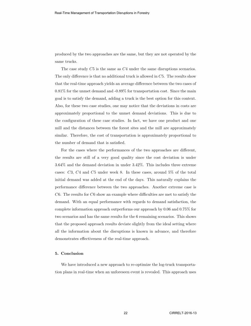
produced by the two approaches are the same, but they are not operated by the

same trucks.

The case study C5 is the same as C4 under the same disruptions scenarios.

The only difference is that no additional truck is allowed in C5. The results show

that the real-time approach yields an average difference between the two cases of

0.81% for the unmet demand and -0.89% for transportation cost. Since the main

goal is to satisfy the demand, adding a truck is the best option for this context.

Also, for these two case studies, one may notice that the deviations in costs are

approximately proportional to the unmet demand deviations. This is due to

the configuration of these case studies. In fact, we have one product and one

mill and the distances between the forest sites and the mill are approximately

similar. Therefore, the cost of transportation is approximately proportional to

the number of demand that is satisfied.

For the cases where the performances of the two approaches are different,

the results are still of a very good quality since the cost deviation is under

3.64% and the demand deviation in under 3.42%. This includes three extreme

cases: C3, C4 and C5 under week 8. In these cases, around 5% of the total

initial demand was added at the end of the days. This naturally explains the

performance difference between the two approaches. Another extreme case is

C6. The results for C6 show an example where difficulties are met to satisfy the

demand. With an equal performance with regards to demand satisfaction, the

complete information approach outperforms our approach by 0.06 and 0.75% for

two scenarios and has the same results for the 6 remaining scenarios. This shows

that the proposed approach results deviate slightly from the ideal setting where

all the information about the disruptions is known in advance, and therefore

demonstrates effectiveness of the real-time approach.

5. Conclusion

We have introduced a new approach to re-optimize the log-truck transporta-

tion plans in real-time when an unforeseen event is revealed. This approach uses


22 CIRRELT-2016-13

a time-space network to represent the evolution of the transportation network

over time and the changes it undergoes following a disruption. The allowed trips

and loading and unloading operations are used as an input for the mathemat-

ical model. The latter is solved to obtain a new transportation plan. Ease of

deployment of this new plan is taken into account through ensuring the conti-

nuity of trips that are in progress when the disruption is revealed unless they

are directly impacted by the disruption. A simulation model was developed to

generate the unforeseen events for real applications provided by FPInnovations.

Compared to a complete information scenario where disruptions are assumed to

be known in advance, the proposed approach produces very good results. Also,

the mathematical model was solved in a few seconds and is thus well suited for

a real-time context.

Future work involves using a heterogeneous fleet of trucks. The presence of

trucks with a loader onboard may give more recourse strategies especially when

facing loader breakdowns at forest sites or mills. The approach proposed in

this paper could be adapted to this context. The time-space network could be

used to represent the disruptions impacts on the forest supply chain. However,

since the trucks may have different capacities and loading constraints, one must

duplicate the arcs for each truck class. This will increase the size of the problem.

In this context, column generation could be used for solving this problem.

References

[1] A. Weintraub, C. Romero, Operations research models and the manage-

ment of agricultural and forestry resources: a review and comparison, In-

terfaces 36 (5) (2006) 446–457.

[2] S. D’Amours, M. Ronnqvist, A. Weintraub, Using operational research for

supply chain planning in the forest products industry, INFOR: Information

Systems and Operational Research 46 (4) (2008) 265–281.

[3] M. Ronnqvist, Optimization in forestry, Mathematical programming 97 (1-

2) (2003) 267–284.


CIRRELT-2016-13 23

[4] D. L. Martell, E. A. Gunn, A. Weintraub, Forest management challenges for

operational researchers, European journal of operational research 104 (1)

(1998) 1–17.

[5] M. Ronnqvist, S. D’Amours, A. Weintraub, A. Jofre, E. Gunn, R. G.

Haight, D. Martell, A. T. Murray, C. Romero, Operations research chal-

lenges in forestry: 33 open problems, Annals of Operations Research 232 (1)

(2015) 11–40.

[6] N. El Hachemi, M. Gendreau, L.-M. Rousseau, A heuristic to solve the syn-

chronized log-truck scheduling problem, Computers & Operations Research

40 (3) (2013) 666–673.

[7] M. Gronalt, P. Hirsch, Log-truck scheduling with a tabu search strategy,

in: Metaheuristics, Springer, 2007, pp. 65–88.

[8] M. Palmgren, M. Ronnqvist, P. Varbrand, A near-exact method for solv-

ing the log-truck scheduling problem, International Transactions in Oper-

ational Research 11 (4) (2004) 447–464.

[9] G. Rix, L.-M. Rousseau, G. Pesant, A column generation algorithm for tac-

tical timber transportation planning, Journal of the Operational Research

Society 66 (2) (2014) 278–287.

[10] A. Weintraub, R. Epstein, R. Morales, J. Seron, P. Traverso, A truck

scheduling system improves efficiency in the forest industries, Interfaces

26 (4) (1996) 1–12.

[11] S. Linnainmaa, J. Savola, O. Jokinen, Epo: A knowledge based system

for wood procurement management., in: Proceedings of the 7th Innovative

Applications of Artificial Intelligence conference, 1995, pp. 107–113.

[12] J.-F. Audy, S. D’Amours, M. Ronnqvist, Planning methods and decision

support systems in vehicle routing problems for timber transportation: A

review, Tech. Rep. CIRRELT-2012-38, CIRRELT (2012).


24 CIRRELT-2016-13

[13] D. Carlsson, M. Ronnqvist, Supply chain management in forestry—-case

studies at sodra cell ab, European Journal of Operational Research 163 (3)

(2005) 589–616.

[14] T. G. Crainic, M. Gendreau, J.-Y. Potvin, Intelligent freight-transportation

systems: Assessment and the contribution of operations research, Trans-

portation Research Part C: Emerging Technologies 17 (6) (2009) 541–557.

[15] M. Ronnqvist, D. Ryan, Solving truck despatch problems in real time,

in: Proceedings of the 31st annual conference of the operational research

society of New Zealand, Vol. 31, 1995, pp. 165–172.

[16] M. Ronnqvist, Or challenges and experiences from solving industrial appli-

cations, International Transactions in Operational Research 19 (1-2) (2012)

227–251.

[17] N. Secomandi, F. Margot, Reoptimization approaches for the vehicle-

routing problem with stochastic demands, Operations Research 57 (1)

(2009) 214–230.

[18] C. Novoa, R. Storer, An approximate dynamic programming approach for

the vehicle routing problem with stochastic demands, European Journal of

Operational Research 196 (2) (2009) 509–515.

[19] D. Carlsson, M. Ronnqvist, Backhauling in forest transportation: models,

methods, and practical usage, Canadian Journal of Forest Research 37 (12)

(2007) 2612–2623.

[20] N. El Hachemi, I. El Hallaoui, M. Gendreau, L.-M. Rousseau, Flow-based

integer linear programs to solve the weekly log-truck scheduling problem,

Annals of Operations Research (2014) 1–11.

[21] P. L’Ecuyer, L. Meliani, J. Vaucher, Ssj: a framework for stochastic simu-

lation in java, in: Proceedings of the 34th conference on Winter simulation:

exploring new frontiers, Winter Simulation Conference, 2002, pp. 234–242.


CIRRELT-2016-13 25

real-time management of transportation disruptions in forestry · real-time management of...

Documents