real estate investors and the boom and bust of the us ... · real estate investors and the boom and...
TRANSCRIPT

Real Estate Investors and the Boom and Bust of the
US Housing Market∗
Zhenyu Gao Wenli Li†
September 2012(Preliminary and Comments Welcome)
Abstract
This paper studies residential real estate investors and their relationship with
local house price movement using several comprehensive micro data on mortgage
application and performance. The paper makes two contributions to the growing
literature on the recent boom and bust of the US housing market. First, using
mortgage application data, we document the important role played by real es-
tate investors. We show that the fraction of mortgage applications for investment
homes rises significantly during the house price run-up and falls sharply during
the house price decline and the pattern is more pronounced for the bubble states
(Arizona, Florida, and Nevada). More importantly, the majority of investment
mortgage borrowers are prime instead of subprime borrowers and they are less
likely to use risky mortgage contracts with adjustable-rate or interest-only than
their subprime primary mortgage counterparts. Second, we find that while rela-
tive demand for investment housing responds to past house price changes up to
10 months, it contributes significantly to changes in local house prices especially
during the pre-crisis period. For the post-crisis period, we show that investors are
more likely to default or being foreclosed on than primary home owners. We argue
that this tendency deteriorated the housing bust.
Keywords: Mortgage crisis, investment housing, house prices, default
∗We thank Wei Xiong and seminar particpants at the Federal Reserve Bank of Philadelphia andPrinceton University for their comments. The views expressed here are those of the authors. They donot necessarily reflect those of the Federal Reserve Bank of Philadelphia or the Federal Reserve System.†Zhenyu Gao: Department of Economics, Princeton University. [email protected]. Wenli Li:
Research Department, Federal Reserve Bank of Philadelphia. [email protected].
1
1 Introduction
The dramatic house price movement of the last decade has led to an increasing liter-
ature that is devoted to the study of residential housing. Almost all of the studies,
however, have focused on owner-occupied housing despite that over 14 percent of US
households also own other residential properties.1 In this paper, we provide a comprehen-
sive empirical description of the characteristics of these households and their activities
(purchasing, loan performance, etc.) and contrast them with those of owner-occupied
housing.2 We are particularly interested in the relationship between investment housing
and local house prices during the recent housing cycle. Understanding this relationship
is important for the design and implementation of policies aimed at reviving the current
housing market and preventing future crisis.
The key difference between owner-occupied housing and investment housing is that
while owner-occupied housing provides housing services to its owner and at the same
time serves as an investment vehicle, investment housing functions mostly as an invest-
ment asset. Consequently, transaction and default cost (monetary cost, emotional cost,
etc.) is lower for real estate investors than for owner-occupants. A direct implication
is then the demand for investment housing is more price elastic than that for owner-
occupied housing. I.e., real estate investors are more likely to buy and sell as house price
changes and they are more likely to default on their mortgages when housing conditions
deteriorate. Furthermore, they are likely to be price setters in local housing market.
Our micro data come from several sources. The primary source is the Home Mortgage
Disclosure Act (HMDA) which provides us with individual monthly mortgage application
and origination information. Using HMDA, we show that at the national level there was a
huge run-up in the fraction of mortgage applications for investment housing between 2000
and 2005. At the peak in 2005, the rate reached over 16 percent from its low of 6 percent
in 2000. After 2005, however, the rate came down sharply while house prices continued to
climb until the second half of 2006. We observe the same pattern with similar magnitude
when we construct the ratio by the origination amount. For the states that have the most
housing boom and the worst housing bust (Arizona, California, Florida, and Nevada),
with the exception of California, the run-up and the subsequent decline in the relative
1There are two types of nonowner-occupied residential properties, vacation or future retirementhomes and investment homes whose owners intend to resell the property without the intention of livingin the house. In both cases, the house may be rent out when the owners are not occupying the house.The line between the two categories, however, can be fine as homeowners can easily turn vacation andretirment homes into investment homes.
2Throughout the paper, we will abuse the notation and use nonowner-occupied housing and invest-ment housing interchangeably.
2
demand are more evident.3 At the peak, over one-fourth of the loan applications as well
as loan originations are for investment housing. Only a small fraction of the borrowers
for investment housing are subprime borrowers (less than 15 percent at the peak). This
is consistent with the findings from the Survey of Consumer Finances (SCF) where we
show that real estate investors tend to have higher income and more educated than
primary homeowners. They also have lower mortgage loan-to-value ratios and overall
deb-to-asset ratios. Furthermore, using information from LPS Applied Analytics, Inc.
(LPS) and Corelogic Inc. (Corelogic), we show that, counter to conventional wisdom,
real estate investors are actually less likely to use exotic mortgage products (adjustable
rate mortgages, interest-only mortgages, etc.) than their subprime counterparts though
they are more likely to use these products than their prime counterparts.
Using instrumental variable approach, we show that while the relative demand of
investment housing measured by the share of investment housing mortgage application
in total application responds positively to past local house price movements at the zip
code level up to 10 months, it contributes to local house price movements with both
economic and statistical significance especially during the pre-crisis period where a 10
percent increase in the relative demand leads to over 6 percent increase in the monthly
house price growth rates. After the crisis, we show that investment home mortgages
are much more likely to default especially those that are also subprime. This tendency
combined with findings in the literature on foreclosure and house prices (Mian, Sufi, and
Trebbi 2010) suggest that investment housing deteriorated housing bust.
Our paper contributes to the burgeoning literature that searches for an explana-
tion for the recent boom-bust pattern in house prices. In particular, the paper is most
closely related to Haughwout, Lee, Tracy Klaauw (2011) who are among the first to
point out the important role played by real estate investors during the housing cycle.4
Our analysis extends Haughwout et al. (2011) along two important dimensions.5 First,
3California is unique in the nation because of Proposition 13. Proposition 13, passed in 1978,established the base year value concept for property tax assessments. Under Proposition 13, the 1975-1976 fiscal year serves as the original base year used in determining the assessment for real property.Thereafter, annual increases to the base year value are limited to the inflation rate, as measured by theCalifornia Consumer Price Index, or two percent, whichever is less. A new base year value, however, isestablished whenever a property has had a change in ownership or has been newly constructed. Thisproposition obviously is not conducive to real estate investors as they frequently buy and sell properties.Other states such as Florida and New York have adopted similar policies. However, they are far lessrestricting.
4See Wheaton and Nechayev (2006). For industry note on investor behavior, see, for example,http://www.calculatedriskblog.com/2005/04/housing-speculation-is-key.html.
5Instead of relying on households’self-reported occupancy type, Haughwout et al. (2011) back outhousing occupancy type by counting the number of first liens held by households using credit bureaudata. Their methodology allows them to overcome the potential underreporting bias of investmenthousing by owners. Indeed, the rate of investment housing demand by origination amount is about 10
3

by using HMDA, we are able to observe investment housing demand directly (mort-
gage applications as captured by HMDA) in addition to mortgage originations at higher
frequency and more comprehensively. Additionally, our study of both prime and sub-
prime mortgage loan-level data allows us to reach a different conclusion concerning the
riskiness of investment housing mortgage borrowers.6 These households are much more
likely to be prime borrowers and they are less likely to use risky mortgage products than
their subprime counterparts. Second and more importantly, we explore the empirical
relationship between investment housing and local house prices and ask to what extent
investment housing has contributed to the housing boom and deteriorated the housing
bust. This additional analysis is crucial in helping us better understand the housing
cycle and thus shed light on relevant policy debates. Besides Haughwout et al. (2011),
another closely related paper is Robinson and Todd (2010) where they examine the role
non-owner occupied properties played during the foreclosure crisis.
Other papers that investigate speculative housing behavior include Barlevy and
Fisher (2011), Bayer, Geissler, and Roberts (2011), Chinco and Mayer (2011), and Choi,
Hong, and Shenkman (2011). Barlevy and Fisher (2011) describe a rational expecta-
tions model in which speculative bubbles in house prices can emerge and when they
emerge, both speculators and lenders prefer interest-only mortgages. They test their
theory using city level data. Bayer et al. (2011) examine the role of speculators and
middlemen in Los Angeles and find that middlemen who buy and sell many houses op-
erate equally during booms and busts, but that speculators who buy and sell a smaller
number of houses appear to try unsuccessfully to time the market and are strongly as-
sociated with neighborhood price instability. Chinco and Mayer (2011) study the price
impact of adding noise traders in the form of distant speculators to a financial market
using unique transactions level data on US residential housing. They find that adding
out of town speculators to a market causes excess house price appreciation and that
out of town speculators likely earn lower returns than local purchasers. Choi, Hong,
and Sheinkman (2011) develop and empirically test a speculation-based theory of home
improvements. They find that improvements are increasing and convex in home prices.
And the change in the recoup ratio (the ratio of resale value of improvements to con-
struction costs) is negatively correlated with construction cost growth controlling for
home price appreciation.
percentage points higher in their data than in ours. One potential shortcoming of their approach isthat there may be double counting for those households who are in the process of selling and buyinghouses and, therefore, may have two mortgages on their account during the transition.
6Since Corelogic ABS data consists of subprime and alt-A borrowers only, the match between thecredit bureau data and Corelogic conducted in Haughwout et al. (2011) does not capture investmenthousing activities among prime borrowers.
4

Another strand of the literature, notably, Mian and Sufi (2009), Keys, Mukherjee,
Seru, and Vig (2009), Adelino, Gerardi, and Willen (2009), Jiang, Nelson, and Vytlacil
(2010), and Elul (2011), focuses on subprime lending and mortgage securitization as the
leading cause of the housing bubble. That literature has generally found that the ex-
pansion in mortgage credit to subprime borrowers is closely correlated with the increase
in securitization of subprime mortgages and this increase in turn leads to poor perfor-
mance of the securitized loans. Following up on this literature, Piskorski, Seru, and Vig
(2010), and Agarwal, Amromin, Ben-David, Chomsisengphet, and Evanoff (2011) later
show that whether a delinquent loan is securitized or not may also affect the ease of
modifying it and hence of avoiding foreclosure.
Finally, the paper also has important implications for the macro housing literature
that studies issues such as house price determination, household portfolio choice, and
the effect of government involvement in the housing market. This literature has focused
exclusively on the primary housing market.7 Put it simply, the only margin along which
households adjust their housing is by moving from renting to owning or vice versa.
Many primary home purchasers make “churn”moves from one house to another —hence
a transaction may have little impact on market vacancy and the overall housing market.
A purchase/sale by real estate investors by comparison can subtract or add more directly
to vacancy and hence net housing supply. In other words, our research suggests that
exclusion of investment housing may bias down the response of house prices to other
shocks and households’ adjustment of consumption and portfolio in the presence of
house price shocks. In our view, a housing model that allows for investment housing
is perhaps a more appropriate framework for understanding house price dynamics and
studying housing policy issues.
The remainder of the paper is structured as follows. Section 2 develops a theoretical
model of owner-occupied and investment housing demand and derives several model
implications. Section 3 describes the data and provides initial empirical analysis of the
residential real estate investors. Section 4 presents the empirical analysis with a focus
on the relationship between investment housing demand and local house price dynamics.
Section 5 concludes the paper.
7To name a few of the papers in the literature, Flavin and Yamashita (2002), Cocco (2005), Yao andZhang (2005), Li and Yao (2007), Chambers, Garriga, and Schlagenhauf (2009), Favilukis, Ludvigson,and Van Nieuwerburgh (2009), and Kiyotaki, Michaelides, and Nikolov (20011).
5

2 A Simple of Theory of Owner-occupied and In-
vestment Housing
We develop a simple model of housing demand that differentiates between primary homes
and investment homes in this section. The purpose is to sort out the different economic
forces such as income, financial constraints, and expected house price changes on the
relative demand of investment housing to primary housing and the feedback effect of the
relative demand on house prices. Derived model implications help guide our subsequent
empirical analysis.
2.1 The Setup
Consider a household that lives for two periods and has a quasi-linear utility function,
(1) α log c+ (1− α) log h+ Ew,
where c represents non-housing consumption, h represents housing services derived from
primary residence, w denotes liquid wealth at the second period, and 1−α (0 ≤ α ≤ 1)
is the housing preference parameter (weight). The timing of the events is as follows.
Households start period 1 with income y1 and face house price p1. The household
then decides on consumption c, the amount of primary housing h, and the amount of
investment housing s to purchase. We rule out short sales by restricting h, s ≥ 0. To
purchase a house, the household has to put down a fraction θ (0 < θ < 1) of the
house value as down payment. We do not allow for other forms of borrowing. Let r
denote the risk free interest rate lenders have to offer to outside depositors that are not
modeled here, rh and rs denote the mortgage rate lenders charge on primary housing
and investment housing, respectively. Additionally, there is a risk management cost of
ψ (ψ ≥ 0) associated with each unit of loans made. We assume a competitive lending
market.
At the beginning of the second period, the household learns the new house price
p2 as it decides whether to repay the mortgage debt or to walk away from the house
by defaulting. If it repays the mortgage debt, it receives the remaining house equity.
If it defaults, it suffers a loss of a proportional cost ch for primary housing and cs for
investment housing. We assume that 0 < cs < ch < 1 to capture the additional cost
(monetary as well as emotional) associated with defaulting on ones’primary residence.
We denote the household’s default decision on its primary residence and investment
housing by dh and ds, respectively, where dh(ds) takes the value of 1 if the household
defaults on its primary (investment) mortgages and 0 otherwise. Additionally, we assume
6

that selling one’s primary residence requires a cost that is proportional (0 < δ < 1) to
the house value and normalize the selling cost for investment housing to 0. Again, this
assumption is to capture the additional monetary cost one incurs when moving its family
out of its primary residence as well as the emotional cost associated with having to leave
one’s home.
The household’s optimization problem can then be written as,
max{h,s,a,dh,ds}
{α log c+ (1− α) log h+ Ew}
s.t. θp1(h+ s) + c ≤ y1,(2)
w = (1− dh)[(1− δ)p2h− rh(1− θ)p1h]− dhchp2h+ (1− ds)[p2s− rs(1− θ)p1s]− dscsp2s,(3)
h, s, c ≥ 0, dh, ds ∈ {0, 1},(4)
where equation (2) is the first period budget constraint. Equation (3) is the second period
budget constraint. The term (1− dh)[(1− δ)p2h− rh(1− θ)p1h] is the home equity after
repaying the debt when the household repays the debt on the primary house, and dhchp2h
is the cost of defaulting on the primary mortgage. Similarly, (1− ds)[p2s− rs(1− θ)p1s]is the home equity after repaying the debt when the household repays the debt on the
investment house, and dscsp2s is the cost of defaulting on the investment mortgage.
Lenders’break-even conditions on lending to the primary house and lending to the
investment housing are as follows,
(r + ψ)(1− θ)p1h = E[(1− dh)rh(1− θ)p1h+ dhp2h],(5)
(r + ψ)(1− θ)p1s = E[(1− ds)rs(1− θ)p1s+ dsp2s].(6)
The left hand side of the equations represents the opportunity cost of making the mort-
gages while the right hand side the expected payoffs.
2.2 Partial Equilibrium Solutions
In appendix A, we provide first order conditions for the problem outlined above. From
the first order conditions, we obtain the following results immediately,
Result 1 Everything else the same, relatively rich households purchase investmenthousing and the richer the household is, the more investment housing it purchases.
7

Under the assumption that no default occurs for either the primary and investment
mortgages, we have if y1 ≥ 1−αδEp2
+ αE[p2−(r+ψ)(1−θ)p1] ,
h =1− αδEp2
,(7)
s =y1θp1− α
E[p2 − (r + ψ)(1− θ)p1]− 1− αδEp2
,(8)
and hence
Result 2. Under the assumption that no default occurs for either primary or invest-ment homes, the relative demand for investment housing decreases with the risk
management cost ψ but increases with the expected second period house price rate
of appreciation E p2p1.
When defaults do occur, under the assumption that ch > cs + δ we have,
Result 3. Households are more likely to default on investment houses than primaryhouses holding everything else constant.
2.3 Endogenizing First-Period House Price
A simple way to endogenize the first period’s house price determination p1 is to assume
that there is a fixed supply of housing, L, and a measure one of households with first
period income y1 following the distribution F (y1). The market clearing condition is,∫y1
(h+ s)dF (y1) = L.
One can show that any factor that leads to higher housing demand in general would
lead to higher first period price. Among those factors, as we have shown, improvement in
first period income, risk management fees, and expected second house price appreciation
rate would lead to disproportional increases in the demand in investment housing.
Result 4. Higher relative demand for investment housing is associated with higher firstperiod prices.
In Appendix B, we provide a numerical example where we allow for default and
endogenize first period house price. The prior results carry through. The intuition for
these four results remains with several extensions of the model. For example, one can
allow for dividend payment with investment housing in the first period or an additional
investment opportunity, bond or stock, between the two periods.
8
3 Data and Descriptive Analysis
3.1 Data Source
The data for the study come from four sources: HomeMortgage Disclosure Act (HMDA),
Survey of Consumer Finances (SCF), LPS Applied Analytics, Inc. (LPS), and Corelogic
Inc. (Corelogic). HMDA covers almost all mortgage applications as well as originations
in US. It records each applicant’s final status (denied/approved/originated), purpose of
borrowing (home purchase/refinancing/home improvement), occupancy type (primary
residence/second or investment homes), loan amount, race, sex, income, as well as lender
institution.8 The Survey of Consumer Finances (SCF) is a triennial cross-sectional
survey of US families except over 2007—2009 periods when the survey collected panel
data. The data include information on families’balance sheets, pensions, income, and
demographic characteristics. Households report their holdings of primary residential
property and non-primary residential property separately. However, like HMDA, the
survey does not distinguish between second and investment homes.
Our prime mortgage sample comes from LPS which provides information from home-
owners’mortgage applications concerning their financial situation, characteristics of the
property, terms of the mortgage contract, and information about securitization, plus
updates on whether homeowners paid in full or defaulted, whether lenders started fore-
closure and whether the home was sold in foreclosure. LPS covers some two-thirds of
installment-type loans in the residential mortgage servicing market. Our subprime mort-
gage sample comes from Corelogic which provides similar information as LPS. CoreLogic
covers nearly all mortgages that were in non-agency subprime mortgage securitization.
According to Ashcraft and Schuermann (2008, table 1), around 72 percent of all sub-
prime mortgages issued during our period were included in non-agency securitization,
making our sample fairly representative of all subprime mortgages. Both LPS and Core-
logic are at the monthly frequency and distinguish between second home mortgages and
investment home mortgages. Our zip code level house price indexes come from Corelogic.
These price indexes are aggregated over all housing transactions, those with mortgages
(prime as well as subprime) and those without.
For the part of our analysis that uses HMDA, we study all purchase mortgages
applied or originated since HMDA did not report on lien type before 2004. For the
analysis using LPS and Corelogic, we focus on first-lien purchase mortgages to avoid
double counting on properties. Due to data size, we only follow a 2 percent random
sample of these mortgage loans over time, LPS as well as Corelogic, until they are
8A lender who does not do business in any msa does not need to report (e.g., small communitybanks) to HMDA.
9
repaid in full, go into default, or until the sample period ends which is October 2011
for both data sets. Note that our analysis includes all family types, one-to-four family
dwelling as well as multifamily dwelling. Because one-to-four family dwelling accounted
for over 95 percent of total mortgage applications and over 97 percent of second and
investment home mortgage applications during our sample period, our results are not
affected much if we focus our analysis exclusively on one-to-four family units.
3.2 Relative Demand for Investment Housing
Wemeasure relative demand in investment housing using two surveys, SCFmeasurement
that is at three-year frequency and limited in coverage and geographic information but
captures owner-occupied and investment housing that are not financed by mortgages,
and HMDA measurement that is at monthly frequency and much more comprehensive
but captures only demand financed by mortgages.
According to Survey of Consumer Finances, from 1989 to 2007, the fraction of house-
holds that own their primary homes increased significantly from 64 percent to 69 percent
while the fraction of households that own other residential properties increased slightly
from 13 percent to 14 percent. In terms of real asset value, however, nonowner-occupied
housing increased by 250 percent, far stripping the increase of 192 percent in owner-
occupied housing suggesting that there had been more demand for investment housing
along the intensive margin than the extensive margin during the housing boom. Interest-
ingly, by 2010, while the fraction of primary homeowners fell to 67 percent, the fraction
of residential investors increased to over 14 percent after a dip in 2009. In terms of asset
value, both property types experienced substantial declines, 23 percent for own-occupied
properties and 22 percent for nonowner-occupied properties.
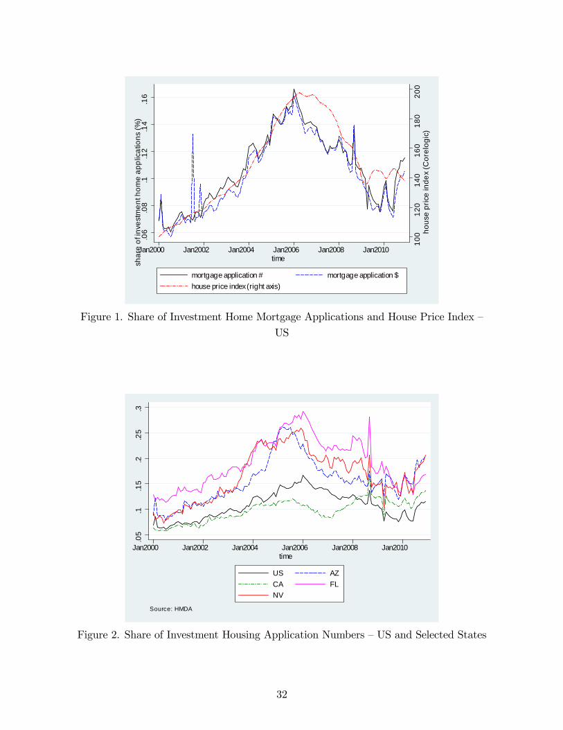
To capture investment housing demand at higher frequency, we turn to HMDA to
construct the following two measures: the fraction of total number of loan applications
that are for investment housing and the fraction of total amount of loan applications
that are for investment housing. We chart the two measures in figure 1. For comparison,
we also chart the real house price indexes provided by Corelogic. We use the headline
consumer price index as the deflator. As can be seen, the relative demand for investment
housing began to increase in 2000 and the increase accelerated at the end of 2003. At
its peak, investment housing accounts for about 16 percent of total loan applications
both in numbers and in dollar amount. What is more, the relative demand peaked in
late 2005, one year ahead of the peak of real house price index. Finally, the relative
demand for investment homes plateaued in 2009 along with house prices but ticked up
substantially since early 2010 while house prices continued to move sideways.
10
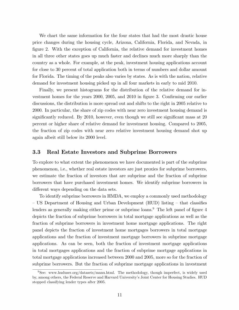
We chart the same information for the four states that had the most drastic house
price changes during the housing cycle, Arizona, California, Florida, and Nevada, in
figure 2. With the exception of California, the relative demand for investment homes
in all three other states goes up much faster and declines much more sharply than the
country as a whole. For example, at the peak, investment housing applications account
for close to 30 percent of total application both in terms of numbers and dollar amount
for Florida. The timing of the peaks also varies by states. As is with the nation, relative
demand for investment housing picked up in all four markets in early to mid 2010.
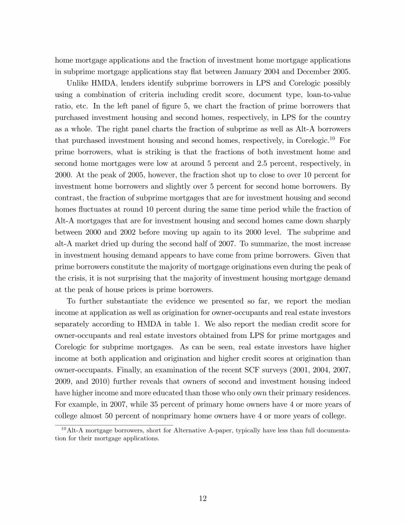
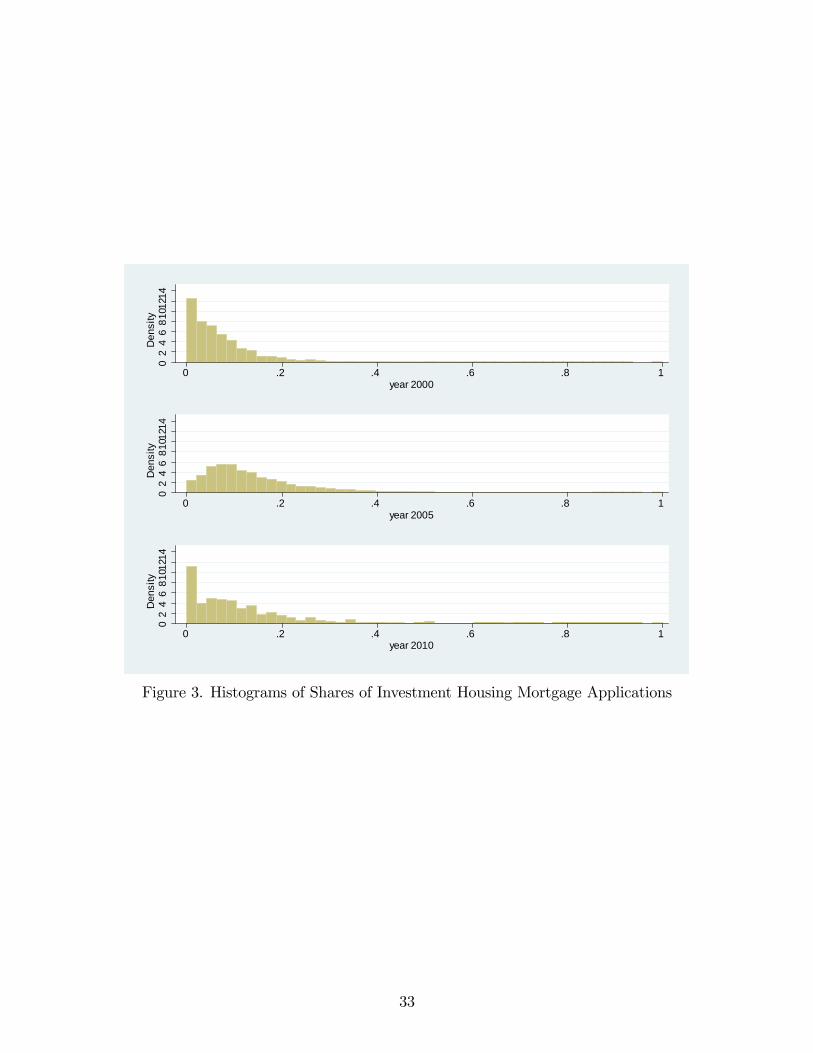
Finally, we present histograms for the distribution of the relative demand for in-
vestment homes for the years 2000, 2005, and 2010 in figure 3. Confirming our earlier
discussions, the distribution is more spread out and shifts to the right in 2005 relative to
2000. In particular, the share of zip codes with near zero investment housing demand is
significantly reduced. By 2010, however, even though we still see significant mass at 20
percent or higher share of relative demand for investment housing. Compared to 2005,
the fraction of zip codes with near zero relative investment housing demand shot up
again albeit still below its 2000 level.
3.3 Real Estate Investors and Subprime Borrowers
To explore to what extent the phenomenon we have documented is part of the subprime
phenomenon, i.e., whether real estate investors are just proxies for subprime borrowers,
we estimate the fraction of investors that are subprime and the fraction of subprime
borrowers that have purchased investment homes. We identify subprime borrowers in
different ways depending on the data sets.
To identify subprime borrowers in HMDA, we employ a commonly used methodology
—US Department of Housing and Urban Development (HUD) listing —that classifies
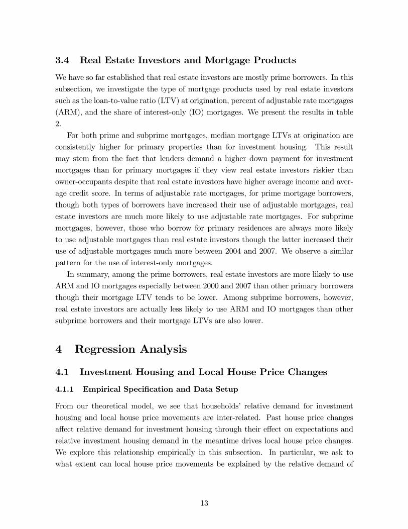
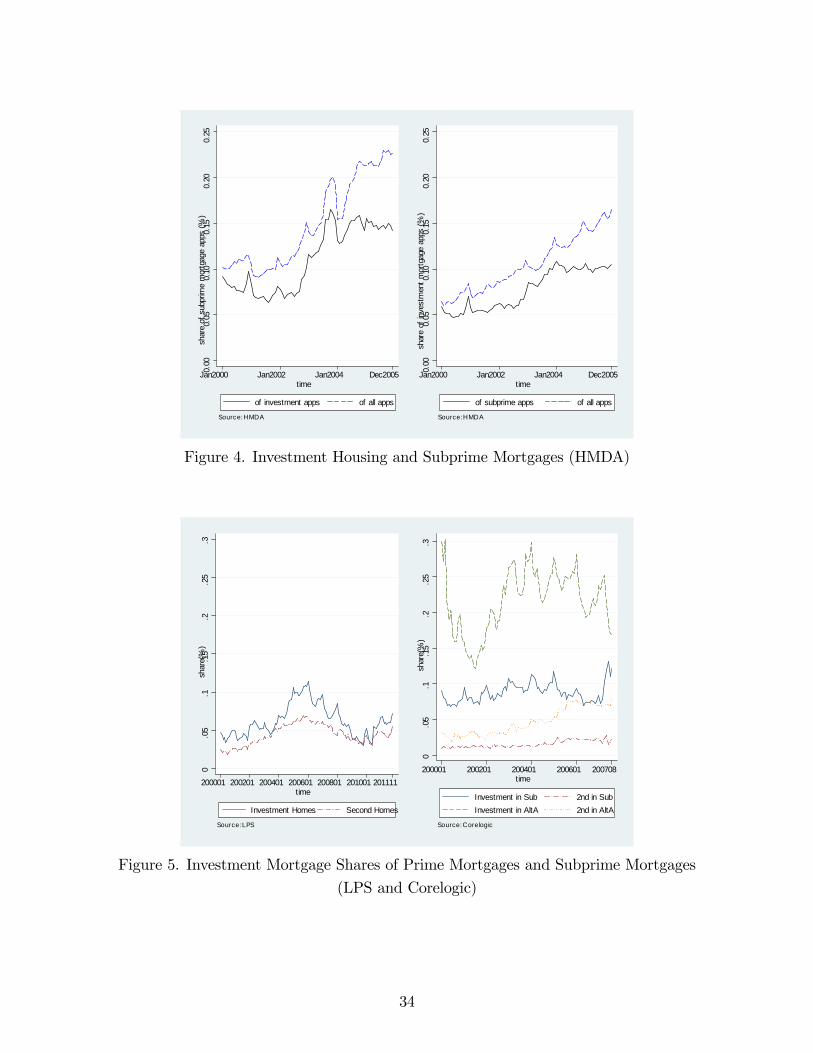
lenders as generally making either prime or subprime loans.9 The left panel of figure 4
depicts the fraction of subprime borrowers in total mortgage applications as well as the
fraction of subprime borrowers in investment home mortgage applications. The right
panel depicts the fraction of investment home mortgages borrowers in total mortgage
applications and the fraction of investment mortgage borrowers in subprime mortgage
applications. As can be seen, both the fraction of investment mortgage applications
in total mortgages applications and the fraction of subprime mortgage applications in
total mortgage applications increased between 2000 and 2005, more so for the fraction of
subprime borrowers. But the fraction of subprime mortgage applications in investment
9See: www.huduser.org/datasets/manu.html. The methodology, though imperfect, is widely usedby, among others, the Federal Reserve and Harvard University’s Joint Center for Housing Studies. HUDstopped classifying lender types after 2005.
11
home mortgage applications and the fraction of investment home mortgage applications
in subprime mortgage applications stay flat between January 2004 and December 2005.
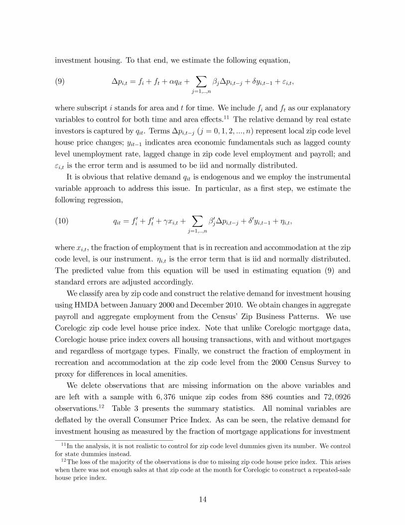
Unlike HMDA, lenders identify subprime borrowers in LPS and Corelogic possibly
using a combination of criteria including credit score, document type, loan-to-value
ratio, etc. In the left panel of figure 5, we chart the fraction of prime borrowers that
purchased investment housing and second homes, respectively, in LPS for the country
as a whole. The right panel charts the fraction of subprime as well as Alt-A borrowers
that purchased investment housing and second homes, respectively, in Corelogic.10 For
prime borrowers, what is striking is that the fractions of both investment home and
second home mortgages were low at around 5 percent and 2.5 percent, respectively, in
2000. At the peak of 2005, however, the fraction shot up to close to over 10 percent for
investment home borrowers and slightly over 5 percent for second home borrowers. By
contrast, the fraction of subprime mortgages that are for investment housing and second
homes fluctuates at round 10 percent during the same time period while the fraction of
Alt-A mortgages that are for investment housing and second homes came down sharply
between 2000 and 2002 before moving up again to its 2000 level. The subprime and
alt-A market dried up during the second half of 2007. To summarize, the most increase
in investment housing demand appears to have come from prime borrowers. Given that
prime borrowers constitute the majority of mortgage originations even during the peak of
the crisis, it is not surprising that the majority of investment housing mortgage demand
at the peak of house prices is prime borrowers.
To further substantiate the evidence we presented so far, we report the median
income at application as well as origination for owner-occupants and real estate investors
separately according to HMDA in table 1. We also report the median credit score for
owner-occupants and real estate investors obtained from LPS for prime mortgages and
Corelogic for subprime mortgages. As can be seen, real estate investors have higher
income at both application and origination and higher credit scores at origination than
owner-occupants. Finally, an examination of the recent SCF surveys (2001, 2004, 2007,
2009, and 2010) further reveals that owners of second and investment housing indeed
have higher income andmore educated than those who only own their primary residences.
For example, in 2007, while 35 percent of primary home owners have 4 or more years of
college almost 50 percent of nonprimary home owners have 4 or more years of college.
10Alt-A mortgage borrowers, short for Alternative A-paper, typically have less than full documenta-tion for their mortgage applications.
12
3.4 Real Estate Investors and Mortgage Products
We have so far established that real estate investors are mostly prime borrowers. In this
subsection, we investigate the type of mortgage products used by real estate investors
such as the loan-to-value ratio (LTV) at origination, percent of adjustable rate mortgages
(ARM), and the share of interest-only (IO) mortgages. We present the results in table
2.
For both prime and subprime mortgages, median mortgage LTVs at origination are
consistently higher for primary properties than for investment housing. This result
may stem from the fact that lenders demand a higher down payment for investment
mortgages than for primary mortgages if they view real estate investors riskier than
owner-occupants despite that real estate investors have higher average income and aver-
age credit score. In terms of adjustable rate mortgages, for prime mortgage borrowers,
though both types of borrowers have increased their use of adjustable mortgages, real
estate investors are much more likely to use adjustable rate mortgages. For subprime
mortgages, however, those who borrow for primary residences are always more likely
to use adjustable mortgages than real estate investors though the latter increased their
use of adjustable mortgages much more between 2004 and 2007. We observe a similar
pattern for the use of interest-only mortgages.
In summary, among the prime borrowers, real estate investors are more likely to use
ARM and IO mortgages especially between 2000 and 2007 than other primary borrowers
though their mortgage LTV tends to be lower. Among subprime borrowers, however,
real estate investors are actually less likely to use ARM and IO mortgages than other
subprime borrowers and their mortgage LTVs are also lower.
4 Regression Analysis
4.1 Investment Housing and Local House Price Changes
4.1.1 Empirical Specification and Data Setup
From our theoretical model, we see that households’ relative demand for investment
housing and local house price movements are inter-related. Past house price changes
affect relative demand for investment housing through their effect on expectations and
relative investment housing demand in the meantime drives local house price changes.
We explore this relationship empirically in this subsection. In particular, we ask to
what extent can local house price movements be explained by the relative demand of
13
investment housing. To that end, we estimate the following equation,
(9) ∆pi,t = fi + ft + αqit +∑
j=1,..,n
βj∆pi,t−j + δyi,t−1 + εi,t,
where subscript i stands for area and t for time. We include fi and ft as our explanatory
variables to control for both time and area effects.11 The relative demand by real estate
investors is captured by qit. Terms ∆pi,t−j (j = 0, 1, 2, ..., n) represent local zip code level
house price changes; yit−1 indicates area economic fundamentals such as lagged county
level unemployment rate, lagged change in zip code level employment and payroll; and
εi,t is the error term and is assumed to be iid and normally distributed.
It is obvious that relative demand qit is endogenous and we employ the instrumental
variable approach to address this issue. In particular, as a first step, we estimate the
following regression,
(10) qit = f ′i + f ′t + γxi,t +∑
j=1,..,n
β′j∆pi,t−j + δ′yi,t−1 + ηi,t,
where xi,t, the fraction of employment that is in recreation and accommodation at the zip
code level, is our instrument. ηi,t is the error term that is iid and normally distributed.
The predicted value from this equation will be used in estimating equation (9) and
standard errors are adjusted accordingly.
We classify area by zip code and construct the relative demand for investment housing
using HMDA between January 2000 and December 2010. We obtain changes in aggregate
payroll and aggregate employment from the Census’Zip Business Patterns. We use
Corelogic zip code level house price index. Note that unlike Corelogic mortgage data,
Corelogic house price index covers all housing transactions, with and without mortgages
and regardless of mortgage types. Finally, we construct the fraction of employment in
recreation and accommodation at the zip code level from the 2000 Census Survey to
proxy for differences in local amenities.
We delete observations that are missing information on the above variables and
are left with a sample with 6, 376 unique zip codes from 886 counties and 72, 0926
observations.12 Table 3 presents the summary statistics. All nominal variables are
deflated by the overall Consumer Price Index. As can be seen, the relative demand for
investment housing as measured by the fraction of mortgage applications for investment
11In the analysis, it is not realistic to control for zip code level dummies given its number. We controlfor state dummies instead.12The loss of the majority of the observations is due to missing zip code house price index. This arises
when there was not enough sales at that zip code at the month for Corelogic to construct a repeated-salehouse price index.
14
homes has a wide range between 0 (e.g., Agawam City in Hapmden County, MA (zip
01001), Drexel Hill in Delaware County, PA (zip 19026), and Calhown in Gordon County,
GA (zip 30701)) and 1 (e.g., Laughlin in Clark County, NV (zip 89029), Green Valley
in Pima County, AZ (zip 85622), and Falmouth in Barnstable County, MA (02540))
across zip codes during the sample period. Interestingly, about half of the cases where
the demand for housing comes entirely from investment housing occurred in late 2010
as real estate investors intensified their bid for foreclosed houses.
Similarly, the fraction of employment in recreation and accommodation also varies
from 0 percent to over 69 percent according to the 2000 Census. In particular, Lum-
berton in Burlington county, NJ (zip 08048), Lareda Ranch in Orange County, CA (zip
92694), and Rancho Cordo in Sacramento County, CA (zip 95742) had zero employment
in recreation and entertainment while Atlantic City in Atlantic County, NJ (zip 08205),
Mesquite in Clark County, NV (zip 89027), and Laughlin in Clark County, NV (zip
89029) had over 50 of its employment in recreation and accommodation. There is also
substantial heterogeneity over time and across zip codes in growth rate in payroll em-
ployment and total payrolls. Finally, during our sample period, house prices experienced
both big rises and big declines with the maximum monthly net rate of appreciation being
14 percent and maximum net rate of depreciation being 16 percent.
Before turning to our regression analysis, it is worth pointing out that our instru-
ment, the fraction of employment in recreation and accommodation in 2000 at the zip
code level, is highly positively correlated with the relative demand of investment housing
with an overall correlation coeffi cient of 0.4460. Its correlation with other explanatory
variables, the zip code level aggregate payroll and aggregate employment growth rate,
lagged zip code level house price growth rates, by comparison, is very weak with corre-
lation coeffi cients less than −0.0015.
4.1.2 Results
Table 4 reports our benchmark regression analysis where we proxy the relative demand
by the fraction of mortgage application that are for investment housing and the sample
spans from January 2000 to December 2010. We do not report the coeffi cients on time
and state dummies to save space. As can be seen, in the first stage our instrument, the
fraction of workers in recreation and accommodations in 2000, has significant explanatory
power for the relative demand of investment housing. A 10 percentage point increase
in the fraction leads to 13 percentage point increase in the relative demand. This is
not surprising as the fraction of workers in recreation and accommodation accounts for
differences in amenities. Areas that have a higher fraction of such workers are areas that
attract more tourists and thus are more likely to have vacation and investment housing.
15

The one-month lagged zip code level real aggregate payroll growth rate does not impact
on the relative demand statistically significantly, but zip code level employment growth
rate contributes negatively to the relative demand. This result suggests that second and
investment housing are purchased by households mostly outside the zip code and its
immediate surrounding area where its labor force reside. Put it differently, good local
labor market leads to more primary housing buying and hence lower relative demand
for investment housing in the area these workers reside. Another striking finding is that
relative demand responds positively to past house price appreciation up to 10 months.
Local county level unemployment rates, on the other hand, do not affect much of the
relative demand.
For the second stage analysis, we find that relative demand for investment housing
contributes positively to changes in real house price index with a marginal effect of 0.12.
Specifically, a 10 percentage point increase in the share causes monthly real house price
growth rate to go up by 1.2 percentage points, about 67 percent of the average monthly
house price growth rate between January 2000 and December 2010. Turning to the other
variables, we find that local aggregate employment growth rate and aggregate payroll
growth all contribute positively to house price increases. Furthermore, past house price
changes for the most part also drive current house price changes. Local unemployment
rates, by comparison, are largely inconsequential after we control for other variations.
Table 5 presents pre-crisis regression results. We find much larger positive effects
of lagged house price changes on relative demand for investment housing in the first
stage and a much larger effect of current relative demand on investment housing on
house price growth rate. Specifically, the marginal effects of relative demand on houses
price changes increased by five fold. In other words, a 10 percentage point increase in
the relative demand leads to an increase in growth rates of 6.1 percentage point, about
11 percent of the average monthly house price growth rate between January 2000 and
December 2005. The effects of other variables remain similar to the benchmark.
We conduct additional robustness tests by including MSA level, lagged growth rates
of real average annual rents come from surveys of “Class A”(top-quality) apartments
by Reis, a commercial real estate information company. See Ambrose, Eichholtz, and
Lindenthal (2012) for a comprehensive discussion of the impact of rents on local house
prices. We lose a third of observations because of Reis’limited coverage. We conduct the
whole sample analysis and report the results in table 6. The effects of relative demand
of investment on housing on house price changes are now slightly larger. The relative
demand now responds less to past house price changes and only up to sever months.
The lagged real rent growth rates affect the relative demand for investment housing in
two ways. On the one hand, the higher the rents, the more likely people will chose to
16
own their homes. On the other hand, people are also more likely to buy investment
housing as the dividend payments are higher. Our analysis suggests that the first effect
dominate.
We also find our results robust to an alternative definition of relative demand for
investment housing, the fraction of mortgage application amount that is for investment
housing as seen in table 7.
Finally, anecdotal evidence suggests that many of the investment housing purchase
after the crisis are cash transactions, hence, not captured by HMDA. However, these
transactions occurred most recently. In other words, our 2010 measurement of invest-
ment housing demand may be biased downward. We conduct an additional analysis
restricting our sample to be between January 2000 and December 2009, not surprisingly,
the marginal effect of relative investment housing demand on local house price changes,
at 0.13, is now slightly larger. We do not report the regression analysis here to save
space.
4.2 Mortgage Performance
Because investment housing does not provide direct housing service to its owners, our
theory predicts that households are more likely to default on their mortgages on invest-
ment housing than on their primary mortgages. In this subsection, we use a 2 percent
random sample of the LPS and Corelogic to test this theory for prime and subprime
investment housing mortgages separately. We focus our sample period to from January
1996 to October 2011. In particular, we run the following probit regression
dit = cons+ ωINVi + γXit + ξit,
where di is a dummy variable that takes a value of 1 if the mortgage is 90 days or more
delinquent and 0 otherwise, INVi is an indicator for investment housing mortgages,
and Xit include all the other controls including year and state fixed effects, age of the
loan and its square, mortgage loan-to-value ratio at origination; whether the mortgage
has full documentation, whether the mortgage is of fixed rate, whether the mortgage is
interest only, jumbo, or balloon. We restrict our attention to the first 90-day mortgage
delinquency. In other words, we delete a mortgage from the data after it becomes 90-days
delinquent from our sample.
The results are reported in table 8. Holding everything else the same, for prime
mortgages, being investment home raises the 90-day delinquent rate by 1 basis point,
about 4 percent of the average default rate of prime mortgages during the period. The
subprime mortgages, the increase is much larger —16 basis points, close to 20 percent
17
of the average default rate of subprime mortgages. Most of the other variables have the
expected signs for both prime and subprime mortgages, high leverage, jumbo mortgage
(for prime mortgages as all subprime mortgages are jumbo loans), and balloon mortgage
all increase mortgage default rates. By contrast, having full document, fixed-rate mort-
gage and high credit score at origination all reduce mortgage default rates. Loan age,
interestingly, increases the default rates for prime mortgages but decreases the default
rates for subprime mortgages. Finally, past local house price appreciation rate, local
payroll growth, and local employment growth all reduce mortgage default rates.
5 Policy Implications and Conclusion
This paper makes two important contributions to the literature on the recent boom and
bust of the US housing market. First, we document that investment housing played
an important role in the recent housing boom and bust. Moreover, investment homes
are more likely to be prime or near-prime borrowers than subprime borrowers and real
estate investors do not appear to use exotic mortgage products more frequently than
primary borrowers. Then, we study the relationship between the relative demand for
real estate mortgages and local housing market, we show that while past local house
price changes have significantly affected the relative demand for investment housing, the
relative demand also drove the price movement especially during the pre-crisis period.
According to our calculation, from 2000 to 2005, zip code level real house price
growth shot up from an average of 0.39 percent at monthly frequency to 0.74 percent
while the relative demand for investment housing went up from 0.072 to 0.143. Thus,
of the 35 basis point increase, 4.3 (0.611 ∗ (0.143 − 0.072)) basis points or 12 percent
were due to increases in the relative demand for investment housing. Although the drop
in the relative demand contributed relatively little to the overall house price decline
since the onset of the crisis directly, the indirect effect through foreclosure is likely to
be large (Mian, Sufi, and Trebbi 2010). In 2000, the 90 days and more default rate for
prime mortgages is a little under 2 percent and almost all of them came from primary
mortgages as there were hardly any investment home prime mortgages at the time. In
2009, however, prime mortgage default rate climbed up to 9.3 percent, and 7.3 percent
of the default mortgages are investment home mortgages. For subprime mortgages, in
2000 the default rate was about 5 percent and a little over 3 percent of them came from
investment housing mortgages. In 2010, the default rate jumped up to close to 12.3
percent, and over 11 percent of them are investment home mortgages. In 2009, about 72
percent mortgage outstanding is primary according to LPS and Corelogic. Investment
mortgages, thus, caused an increase in default and foreclosure rates of about 0.76 (0.093∗
18

0.073 ∗ 0.72 + 0.123 ∗ (0.11 − 0.03) ∗ 0.28) percentage points, a 7.6 percent increase.
According to Mian, Sufi, and Trebbi (2010), this should have further lowered house
price decline substantially (roughly another 2 percent if we use the -2.693 estimation
coeffi cient from their table 6).
One caveat of our analysis is that we only capture the part of the relative demand
for real estate investing financed by mortgages as many anecdotal evidence suggests
over the last several years, many housing transactions especially investment housing
transactions are bought during foreclosures, are all cash transactions. Furthermore,
we cannot identify the “flippers”—those who bought and sold at high frequency. We
intend to tackle these issues in a future research when housing transaction data become
available to us.
19

Appendix A. First Order Conditions
Let us start with the household’s default decision. Given that the household is
risk-neutral in the second period with no additional income and that this is two-period
mortgage contract which eliminates the option side of the mortgage default,13 it follows
immediately that
dh = 1 if rh(1− θ)p1h > [p2(1− δ) + p2ch]h,(11)
ds = 1 if rs(1− θ)p1s > (p2 + p2cs)s.(12)
In other words, the household will default on its mortgage, primary or investment hous-
ing, if the second period house value plus the default cost falls below the required
mortgage payment. Note that in our model the default decisions and the mortgage rates
are not functions of house sizes.
We can rewrite the household problem as follows after some algebra,
max{h,s,c≥0,0≤dh,ds≤1}
{α log c+ (1− α) log h+ E{(1− dh)[(1− δ)p2h− rh(1− θ)p1h]
− dhchp2h+ (1− ds)[p2s− rsp1(1− θ)s]− dscsp2s}}.(13)
From the first period’s budget constraint, we can replace investment housing demand
s by c and h. Then, we obtain the following first-order conditions (λ is the Lagrangian
multiplier for s ≥ 0),
−θp1αc
+1− αh
+ E{(1− dh)[(1− δ)p2 − rh(1− θ)p1]− dhchp2} = 0,(14)
−θp1αc
+ E{(1− ds)[p2 − rs(1− θ)p1]− dscsp2}+ λ = 0,(15)
λ(y1 − θp1h− c) = 0,(16)
13For example, if the mortgage term were three periods instead of two, then borrowers facing a lowhouse price in the second period can either default then or wait for a possible housing-market recoveryin the third period. Introducing a third period, however, complicates the model substantially.
20
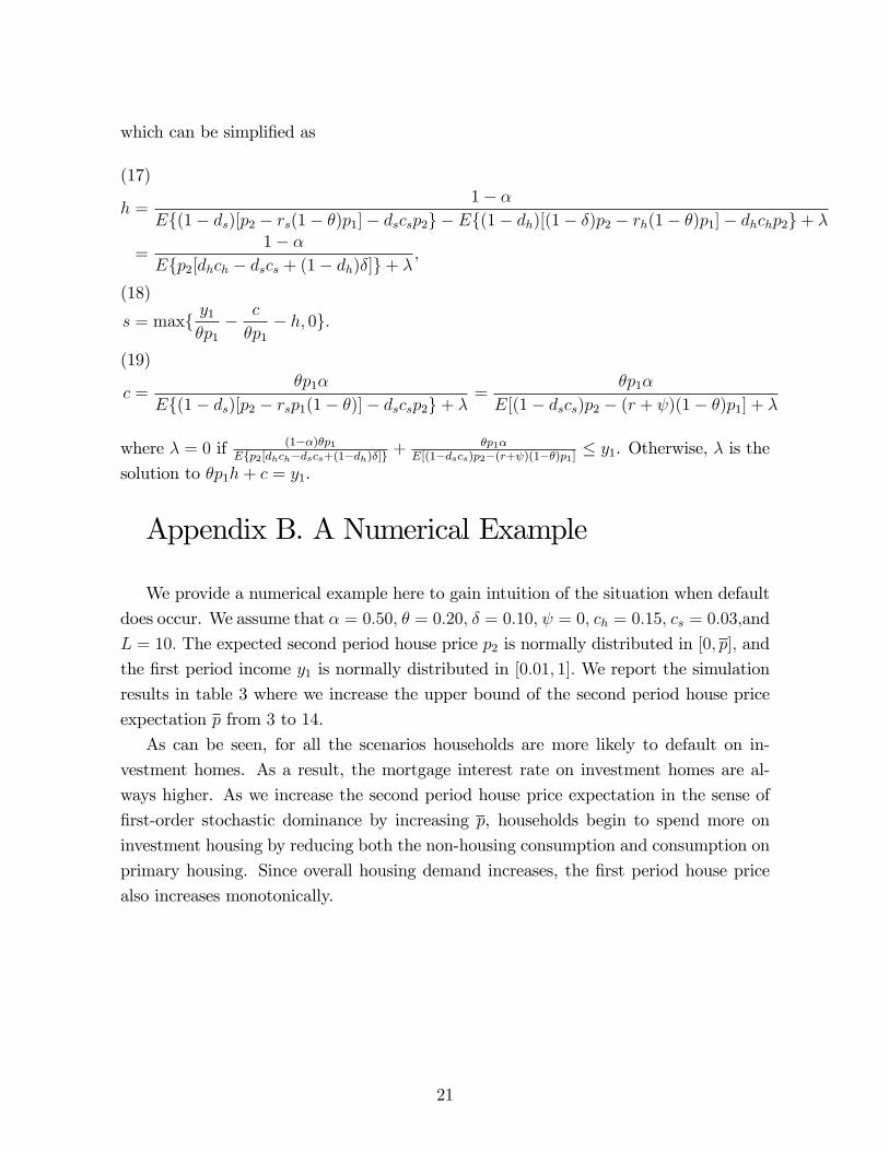
which can be simplified as
h =1− α
E{(1− ds)[p2 − rs(1− θ)p1]− dscsp2} − E{(1− dh)[(1− δ)p2 − rh(1− θ)p1]− dhchp2}+ λ
(17)
=1− α
E{p2[dhch − dscs + (1− dh)δ]}+ λ,
s = max{ y1θp1− c
θp1− h, 0}.
(18)
c =θp1α
E{(1− ds)[p2 − rsp1(1− θ)]− dscsp2}+ λ=
θp1α
E[(1− dscs)p2 − (r + ψ)(1− θ)p1] + λ
(19)
where λ = 0 if (1−α)θp1E{p2[dhch−dscs+(1−dh)δ]} + θp1α
E[(1−dscs)p2−(r+ψ)(1−θ)p1] ≤ y1. Otherwise, λ is the
solution to θp1h+ c = y1.
Appendix B. A Numerical Example
We provide a numerical example here to gain intuition of the situation when default
does occur. We assume that α = 0.50, θ = 0.20, δ = 0.10, ψ = 0, ch = 0.15, cs = 0.03,and
L = 10. The expected second period house price p2 is normally distributed in [0, p], and
the first period income y1 is normally distributed in [0.01, 1]. We report the simulation
results in table 3 where we increase the upper bound of the second period house price
expectation p from 3 to 14.
As can be seen, for all the scenarios households are more likely to default on in-
vestment homes. As a result, the mortgage interest rate on investment homes are al-
ways higher. As we increase the second period house price expectation in the sense of
first-order stochastic dominance by increasing p, households begin to spend more on
investment housing by reducing both the non-housing consumption and consumption on
primary housing. Since overall housing demand increases, the first period house price
also increases monotonically.
21

References
[1] Adelino, M., Gerardi, K., P. Willen. 2009. “Why Don’t Lenders Renegotiate More
HomeMortgages? Redefaults, Self-Cures and Securitization,”Federal Reserve Bank
of Atlanta Working Paper. 2009-17.
[2] Agarwal, Sumit, Gene Amromin, Itzhak Ben-David, Souphala Chomsisengphet, and
Douglas D. Evanoff. 2011. “The Role of Securitization in Mortgage Renegotiation.”
Journal of Financial Economics, 102(3), pp. 559-578.
[3] Ambrose, Brent W., Piet Eichholtz, and Thies Lindenthal. 2012. “House Prices and
Fundamentals: 355 Years of Evidence.”Manuscript.
[4] Barlevy, Gadi, and Jonas D.M. Fisher. 2011. “Mortgage Choices and Housing Spec-
ulation.”Federal Reserve Bank of Chicago Working Paper June 15, 2011.
[5] Bayer, Patrick, Christopher Geissler, and James W. Roberts. 2011. “Speculators
and Middlemen: The Role of Filppers inthe Housing Market.”National Bureau of
Economic Research Working Paper Series No. 16784.
[6] Chambers, Mattew, Carlos Garriga, and Don Schlagenhauf. 2009. “Accounting for
Changes in the Homeownership Rate.” International Economic Review 50(3), pp.
677-726.
[7] Chinco, Alexander, and Christopher Mayer. 2011. “Noise Traders, Distant Specula-
tors and Asset Bubbles in the Housing Market.”manuscript, Columbia University.
[8] Choi, Hyun-Soo, Harrison Hong, and Jose Scheinkman. 2011. “Speculating on Home
Improvements.”manuscript, Princeton University.
[9] Cocco, Joao. 2005. “Portfolio Choice in the Presence of Housing.”Review of Finan-
cial Studies 18(2), pp. 535-567.
[10] Elul, Ronel. 2011. “Securitization and Mortgage Default.”Federal Reserve Bank of
Philadelphia Working Paper May, 2011.
[11] Favilukis, Jack, Sydney Ludvigson, and Stin Van Favilukis. 2011. “Macroeconomic
Effects of Housing Wealth, Housing Finance, and Limited Risk Sharing in General
Equilibrium,”manuscript, New York University.
[12] Flavin, Marjorie, and Takashi Yamashita. 2002. “Owner-Occupied Housing and the
Composition of the Household Portfolio over the Life-cycle,”American Economic
Review 92, 345-362.
22

[13] Haughwout, Abdrew, Donghoon Lee, Joseph Tracy, and Wilbert van der Klaauw.
2011. “Real Estate Investors, the Leverage Cycle, and the Housing Market Crisis.”
Federal Reserve Bank of New York Staff Report no. 514.
[14] Jiang, Wei, Ashlyn Nelson, and Edward Vytlacil. 2010. “Securitization and Loan
Performance: A Contrast of Ex Ante and Ex Post Relations in the Mortgage Mar-
ket.”manuscript, Columbia University.
[15] Keys, Benjamin, Tanmoy Mukherjee, Amit Seru, and Vikrant Vig. 2010. “Did Se-
curitization Lead to Lax Screening? Evidence from Subprime Loans.”Quarterly
Journal of Economics 125(1), pp.307-362.
[16] Kiyotaki, Nobuhiro, Alex Michaelides, and Kalin Nikolov. 2011. “Winners and
Losers in Housing Markets.”Journal of Money, Credit, and Banking 43(2-3), 255-
296.
[17] Li, Wenli, and Rui Yao. 2007. “The Life-cycle Effects of House Price Changes.”
Journal of Money, Credit, and Banking, pp. 1375-1409.
[18] Mian, Atif, and Amir Sufi. 2009. “The Consequences of Mortgage Credit Expansion:
Evidence from the U.S. Mortgage Default Crisis.”Quarterly Journal of Economics
124(4), pp1449-1496.
[19] Mian, Atif, Amir Sufi, and Francesco Trebbi. 2010. “Foreclosures, House Prices,
and the Real Economy.”NBER working paper 16685.
[20] Piskorski, Tomasz, and Alexei Tchistyi. 2011. “Stochastic House Appreciation and
Optimal Mortgage Lending.”Review of Financial Studies 24(5), pp.1407-1446.
[21] Robbinson, Breck L, and Richard M. Todd. 2010. “The Role of Non-owner-occupied
Homes in the Current Housing and Foreclosure Cycle.” Federal Reserve Bank of
Richmond wp 10-11.
[22] Wheaton, William C., and Gleb Nechayev. 2006. “Past Housing ‘Cycles’and the
Current Housing ‘Boom:’What’s Different This Time?”Manuscript, MIT.
[23] Yao, Rui, and Harold Zhang. 2005. “Optimal Consumption and Portfolio Choices
with Risky Housing and Borrowing Constraints.”Review of Financial Studies 18,
197-239.
23
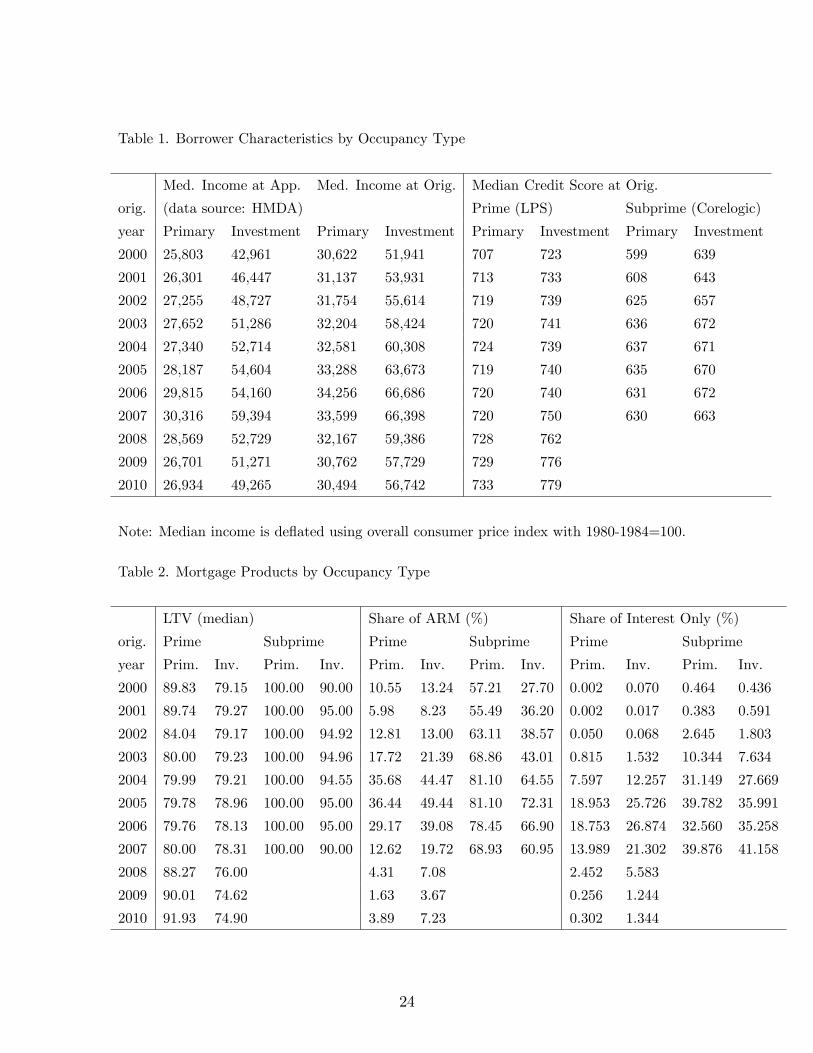
Table 1. Borrower Characteristics by Occupancy Type
Med. Income at App. Med. Income at Orig. Median Credit Score at Orig.
orig. (data source: HMDA) Prime (LPS) Subprime (Corelogic)
year Primary Investment Primary Investment Primary Investment Primary Investment
2000 25,803 42,961 30,622 51,941 707 723 599 639
2001 26,301 46,447 31,137 53,931 713 733 608 643
2002 27,255 48,727 31,754 55,614 719 739 625 657
2003 27,652 51,286 32,204 58,424 720 741 636 672
2004 27,340 52,714 32,581 60,308 724 739 637 671
2005 28,187 54,604 33,288 63,673 719 740 635 670
2006 29,815 54,160 34,256 66,686 720 740 631 672
2007 30,316 59,394 33,599 66,398 720 750 630 663
2008 28,569 52,729 32,167 59,386 728 762
2009 26,701 51,271 30,762 57,729 729 776
2010 26,934 49,265 30,494 56,742 733 779
Note: Median income is deflated using overall consumer price index with 1980-1984=100.
Table 2. Mortgage Products by Occupancy Type
LTV (median) Share of ARM (%) Share of Interest Only (%)
orig. Prime Subprime Prime Subprime Prime Subprime
year Prim. Inv. Prim. Inv. Prim. Inv. Prim. Inv. Prim. Inv. Prim. Inv.
2000 89.83 79.15 100.00 90.00 10.55 13.24 57.21 27.70 0.002 0.070 0.464 0.436
2001 89.74 79.27 100.00 95.00 5.98 8.23 55.49 36.20 0.002 0.017 0.383 0.591
2002 84.04 79.17 100.00 94.92 12.81 13.00 63.11 38.57 0.050 0.068 2.645 1.803
2003 80.00 79.23 100.00 94.96 17.72 21.39 68.86 43.01 0.815 1.532 10.344 7.634
2004 79.99 79.21 100.00 94.55 35.68 44.47 81.10 64.55 7.597 12.257 31.149 27.669
2005 79.78 78.96 100.00 95.00 36.44 49.44 81.10 72.31 18.953 25.726 39.782 35.991
2006 79.76 78.13 100.00 95.00 29.17 39.08 78.45 66.90 18.753 26.874 32.560 35.258
2007 80.00 78.31 100.00 90.00 12.62 19.72 68.93 60.95 13.989 21.302 39.876 41.158
2008 88.27 76.00 4.31 7.08 2.452 5.583
2009 90.01 74.62 1.63 3.67 0.256 1.244
2010 91.93 74.90 3.89 7.23 0.302 1.344
24
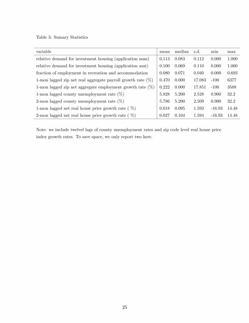
Table 3. Sumary Statistics
variable mean median s.d. min max
relative demand for investment housing (application num) 0.113 0.083 0.112 0.000 1.000
relative demand for investment housing (application amt) 0.100 0.069 0.110 0.000 1.000
fraction of employment in recreation and accommodation 0.080 0.071 0.040 0.000 0.693
1-mon lagged zip net real aggregate payroll growth rate (%) 0.470 0.000 17.083 -100 6377
1-mon lagged zip net aggregate employment growth rate (%) 0.222 0.000 17.851 -100 3588
1-mon lagged county unemployment rate (%) 5.828 5.200 2.528 0.900 32.2
2-mon lagged county unemployment rate (%) 5.786 5.200 2.509 0.900 32.2
1-mon lagged net real house price growth rate ( %) 0.018 0.095 1.593 -16.93 14.48
2-mon lagged net real house price growth rate ( %) 0.027 0.104 1.594 -16.93 14.48
Note: we include twelvel lags of county unemployment rates and zip code level real house price
index growth rates. To save space, we only report two here.
25

Table 4. Investment Housing Demand (num) and House Price Changes (January 2000 - December 2010)
variable Relative Demand for Inv. Housing Real HPI Changes
(first stage) (second stage)
fraction of employ. in rec. and accom. 1.2600 (0.0033)∗∗∗
relative demand for inv. housing 0.1217 (0.0342)∗∗∗
lagged aggregate payroll growth rate -0.0000 (0.0000) 0.0038 (0.0003)∗∗∗
lagged aggregate employment growth rate -0.0001 (0.0000)∗∗∗ 0.0022 (0.0003)∗∗∗
1-mon lagged zip real hpi growth rate 0.0012 (0.0001)∗∗∗ 0.2841 (0.0011)∗∗∗
2-mon lagged zip real hpi growth rate 0.0008 (0.0000)∗∗∗ 0.0022 (0.0012)∗
3-mon lagged zip real hpi growth rate 0.0009 (0.0001)∗∗∗ -0.0489 (0.0012)∗∗∗
4-mon lagged zip real hpi growth rate 0.0008 (0.0001)∗∗∗ 0.0469 (0.0012)∗∗∗
5-mon lagged zip real hpi growth rate 0.0009 (0.0001)∗∗∗ 0.0406 (0.0012)∗∗∗
6-mon lagged zip real hpi growth rate 0.0008 (0.0001)∗∗∗ 0.0267 (0.0013)∗∗∗
7-mon lagged zip real hpi growth rate 0.0007 (0.0001)∗∗∗ 0.0309 (0.0011)∗∗∗
8-mon lagged zip real hpi growth rate 0.0005 (0.0001)∗∗∗ 0.0373 (0.0013)∗∗∗
9-mon lagged zip real hpi growth rate 0.0004 (0.0001)∗∗∗ 0.0385 (0.0013)∗∗∗
10-mon lagged zip real hpi growth rate 0.0003 (0.0001)∗∗∗ 0.0356 (0.0011)∗∗∗
11-mon lagged zip real hpi growth rate 0.00001 (0.0001) 0.0471 (0.0011)∗∗∗
12-mon lagged zip real hpi growth rate -0.0001 (0.0001) 0.0529 (0.0011)∗∗∗
1-mon lagged county unemp. rate -0.0002 (0.0003) -0.0869 (0.0042)∗∗∗
2-mon lagged county unemp. rate -0.0000 (0.0004) 0.0201 (0.0055)∗∗∗
3-mon lagged county unemp. rate 0.0001 (0.0004) 0.0115 (0.0055)∗∗
4-mon lagged county unemp. rate 0.0003 (0.0004) 0.0076 (0.0055)
5-mon lagged county unemp. rate -0.0001 (0.0004) 0.0059 (0.0056)
6-mon lagged county unemp. rate 0.0019 (0.0004)∗∗∗ 0.0018 (0.0056)
7-mon lagged county unemp. rate 0.0005 (0.0004) -0.0152 (0.0056)∗∗
8-mon lagged county unemp. rate 0.0003 (0.0004) -0.0119 (0.0055)∗∗
9-mon lagged county unemp. rate 0.0008 (0.0004)∗∗ 0.0067 (0.0056)
10-mon lagged county unemp. rate -0.0001 (0.0004) -0.0097 (0.0055)∗
11-mon lagged county unemp. rate 0.0005 (0.0004) 0.0055 (0.0055)
12-mon lagged county unemp. rate 0.0005 (0.0003) 0.0068 (0.0042)∗
time dummies yes yes
state dummies yes yes
number of observations 720,926 720,926
R-sq 0.0934 0.4013
Note: *** indicates 1% significance, ** indicates 5% significance, and * indicates 10% significance.
26
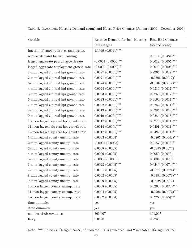
Table 5. Investment Housing Demand (num) and House Price Changes (January 2000 - December 2005)
variable Relative Demand for Inv. Housing Real HPI Changes
(first stage) (second stage)
fraction of employ. in rec. and accom. 1.1949 (0.0041)∗∗∗
relative demand for inv. housing 0.6114 (0.0484)∗∗∗
lagged aggregate payroll growth rate -0.0001 (0.0000)∗∗∗ 0.0018 (0.0005)∗∗∗
lagged aggregate employment growth rate -0.0002 (0.0000)∗∗∗ 0.0019 (0.0006)∗∗∗
1-mon lagged zip real hpi growth rate 0.0027 (0.0001)∗∗∗ 0.2265 (0.0017)∗∗∗
2-mon lagged zip real hpi growth rate 0.0021 (0.0001)∗∗∗ -0.0306 (0.0017)∗∗∗
3-mon lagged zip real hpi growth rate 0.0024 (0.0001)∗∗∗ -0.0702 (0.0017)∗∗∗
4-mon lagged zip real hpi growth rate 0.0024 (0.0001)∗∗∗ 0.0310 (0.0017)∗∗∗
5-mon lagged zip real hpi growth rate 0.0023 (0.0001)∗∗∗ 0.0250 (0.0017)∗∗∗
6-mon lagged zip real hpi growth rate 0.0023 (0.0001)∗∗∗ 0.0160 (0.0017)∗∗∗
7-mon lagged zip real hpi growth rate 0.0022 (0.0001)∗∗∗ 0.0252 (0.0011)∗∗∗
8-mon lagged zip real hpi growth rate 0.0019 (0.0001)∗∗∗ 0.0285 (0.0013)∗∗∗
9-mon lagged zip real hpi growth rate 0.0019 (0.0001)∗∗∗ 0.0284 (0.0013)∗∗∗
10-mon lagged zip real hpi growth rate 0.0017 (0.0001)∗∗∗ 0.0276 (0.0011)∗∗∗
11-mon lagged zip real hpi growth rate 0.0014 (0.0001)∗∗∗ 0.0401 (0.0011)∗∗∗
12-mon lagged zip real hpi growth rate 0.0017 (0.0001)∗∗∗ 0.0482 (0.0011)∗∗∗
1-mon lagged county unemp. rate 0.0003 (0.0004) -0.0265 (0.0042)∗∗∗
2-mon lagged county unemp. rate -0.0001 (0.0005) 0.0157 (0.0073)∗∗
3-mon lagged county unemp. rate 0.0008 (0.0005) -0.0046 (0.0072)
4-mon lagged county unemp. rate 0.0006 (0.0005) 0.0059 (0.0073)
5-mon lagged county unemp. rate -0.0008 (0.0005) 0.0004 (0.0073)
6-mon lagged county unemp. rate 0.0023 (0.0005)∗∗∗ 0.0249 (0.0074)∗∗∗
7-mon lagged county unemp. rate 0.0001 (0.0005) -0.0271 (0.0074)∗∗∗
8-mon lagged county unemp. rate 0.0002 (0.0005) -0.0184 (0.0073)∗∗∗
9-mon lagged county unemp. rate 0.0009 (0.0005)∗ -0.0028 (0.0073)
10-mon lagged county unemp. rate 0.0008 (0.0005) 0.0260 (0.0073)∗∗∗
11-mon lagged county unemp. rate 0.0004 (0.0005) -0.0296 (0.0072)∗∗∗
12-mon lagged county unemp. rate 0.0002 (0.0004) 0.0227 (0.055)∗∗∗
time dummies yes yes
state dummies yes yes
number of observations 361,007 361,007
R-sq 0.0828 0.2236
Note: *** indicates 1% significance, ** indicates 5% significance, and * indicates 10% significance.
27
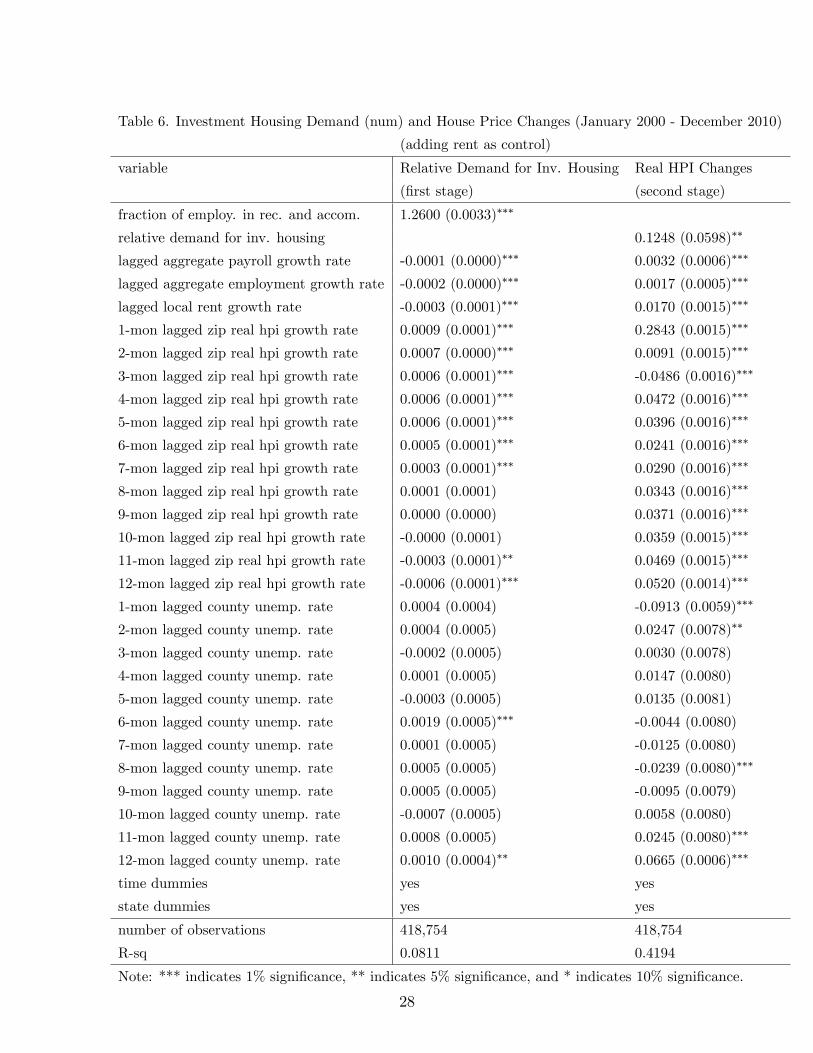
Table 6. Investment Housing Demand (num) and House Price Changes (January 2000 - December 2010)
(adding rent as control)
variable Relative Demand for Inv. Housing Real HPI Changes
(first stage) (second stage)
fraction of employ. in rec. and accom. 1.2600 (0.0033)∗∗∗
relative demand for inv. housing 0.1248 (0.0598)∗∗
lagged aggregate payroll growth rate -0.0001 (0.0000)∗∗∗ 0.0032 (0.0006)∗∗∗
lagged aggregate employment growth rate -0.0002 (0.0000)∗∗∗ 0.0017 (0.0005)∗∗∗
lagged local rent growth rate -0.0003 (0.0001)∗∗∗ 0.0170 (0.0015)∗∗∗
1-mon lagged zip real hpi growth rate 0.0009 (0.0001)∗∗∗ 0.2843 (0.0015)∗∗∗
2-mon lagged zip real hpi growth rate 0.0007 (0.0000)∗∗∗ 0.0091 (0.0015)∗∗∗
3-mon lagged zip real hpi growth rate 0.0006 (0.0001)∗∗∗ -0.0486 (0.0016)∗∗∗
4-mon lagged zip real hpi growth rate 0.0006 (0.0001)∗∗∗ 0.0472 (0.0016)∗∗∗
5-mon lagged zip real hpi growth rate 0.0006 (0.0001)∗∗∗ 0.0396 (0.0016)∗∗∗
6-mon lagged zip real hpi growth rate 0.0005 (0.0001)∗∗∗ 0.0241 (0.0016)∗∗∗
7-mon lagged zip real hpi growth rate 0.0003 (0.0001)∗∗∗ 0.0290 (0.0016)∗∗∗
8-mon lagged zip real hpi growth rate 0.0001 (0.0001) 0.0343 (0.0016)∗∗∗
9-mon lagged zip real hpi growth rate 0.0000 (0.0000) 0.0371 (0.0016)∗∗∗
10-mon lagged zip real hpi growth rate -0.0000 (0.0001) 0.0359 (0.0015)∗∗∗
11-mon lagged zip real hpi growth rate -0.0003 (0.0001)∗∗ 0.0469 (0.0015)∗∗∗
12-mon lagged zip real hpi growth rate -0.0006 (0.0001)∗∗∗ 0.0520 (0.0014)∗∗∗
1-mon lagged county unemp. rate 0.0004 (0.0004) -0.0913 (0.0059)∗∗∗
2-mon lagged county unemp. rate 0.0004 (0.0005) 0.0247 (0.0078)∗∗
3-mon lagged county unemp. rate -0.0002 (0.0005) 0.0030 (0.0078)
4-mon lagged county unemp. rate 0.0001 (0.0005) 0.0147 (0.0080)
5-mon lagged county unemp. rate -0.0003 (0.0005) 0.0135 (0.0081)
6-mon lagged county unemp. rate 0.0019 (0.0005)∗∗∗ -0.0044 (0.0080)
7-mon lagged county unemp. rate 0.0001 (0.0005) -0.0125 (0.0080)
8-mon lagged county unemp. rate 0.0005 (0.0005) -0.0239 (0.0080)∗∗∗
9-mon lagged county unemp. rate 0.0005 (0.0005) -0.0095 (0.0079)
10-mon lagged county unemp. rate -0.0007 (0.0005) 0.0058 (0.0080)
11-mon lagged county unemp. rate 0.0008 (0.0005) 0.0245 (0.0080)∗∗∗
12-mon lagged county unemp. rate 0.0010 (0.0004)∗∗ 0.0665 (0.0006)∗∗∗
time dummies yes yes
state dummies yes yes
number of observations 418,754 418,754
R-sq 0.0811 0.4194
Note: *** indicates 1% significance, ** indicates 5% significance, and * indicates 10% significance.
28

Table 7. Investment Housing Demand (amt) and House Price Changes (January 2000 - December 2010)
variable Relative Demand for Inv. Housing Real HPI Changes
(first stage) (second stage)
fraction of employ. in rec. and accom. 1.3049 (0.0034)∗∗∗
relative demand for inv. housing 0.1175 (0.0330)∗∗
lagged aggregate payroll growth rate -0.0000 (0.0000) 0.0038 (0.0004)∗∗∗
lagged aggregate employment growth rate -0.0001 (0.0000)∗∗ 0.0022 (0.0003)∗∗∗
1-mon lagged zip real hpi growth rate 0.0011 (0.0001)∗∗∗ 0.2841 (0.0012)∗∗∗
2-mon lagged zip real hpi growth rate 0.0009 (0.0001)∗∗∗ 0.0022 (0.0012)∗
3-mon lagged zip real hpi growth rate 0.0008 (0.0001)∗∗∗ -0.0489 (0.0012)∗∗∗
4-mon lagged zip real hpi growth rate 0.0009 (0.0001)∗∗∗ 0.0469 (0.0012)∗∗∗
5-mon lagged zip real hpi growth rate 0.0010 (0.0001)∗∗∗ 0.0406 (0.0012)∗∗∗
6-mon lagged zip real hpi growth rate 0.0009 (0.0001)∗∗∗ 0.02267 (0.0013)∗∗∗
7-mon lagged zip real hpi growth rate 0.0008 (0.0001)∗∗∗ 0.0309 (0.0013)∗∗∗
8-mon lagged zip real hpi growth rate 0.0007 (0.0001)∗∗∗ 0.0373 (0.0012)∗∗∗
9-mon lagged zip real hpi growth rate 0.0006 (0.0001)∗∗∗ 0.0385 (0.0012)∗∗∗
10-mon lagged zip real hpi growth rate 0.0006 (0.0001)∗∗∗ 0.0356 (0.0012)∗∗∗
11-mon lagged zip real hpi growth rate 0.0004 (0.0001)∗∗∗ 0.0471 (0.0012)∗∗∗
12-mon lagged zip real hpi growth rate 0.0003 (0.0001)∗∗∗ 0.0529 (0.0012)∗∗∗
1-mon lagged county unemp. rate -0.0006 (0.0003)∗∗ -0.0869 (0.0042)∗∗∗
2-mon lagged county unemp. rate 0.0004 (0.0004) 0.0201 (0.0055)∗∗∗
3-mon lagged county unemp. rate 0.0001 (0.0004) 0.0115 (0.0044)∗∗
4-mon lagged county unemp. rate 0.0002 (0.0004) 0.0076 (0.0055)
5-mon lagged county unemp. rate -0.0001 (0.0004) 0.0059 (0.0056)
6-mon lagged county unemp. rate 0.0020 (0.0004)∗∗∗ 0.0018 (0.0056)
7-mon lagged county unemp. rate 0.0001 (0.0004) -0.0151 (0.0056)∗∗∗
8-mon lagged county unemp. rate 0.0004 (0.0004) -0.0119 (0.0056)∗∗
9-mon lagged county unemp. rate 0.0008 (0.0005) 0.0067 (0.0057)
10-mon lagged county unemp. rate -0.0000 (0.0004) -0.0098 (0.0056)∗
11-mon lagged county unemp. rate 0.0002 (0.0004) 0.0056 (0.0056)
12-mon lagged county unemp. rate 0.0005 (0.0003) 0.0683 (0.0042)∗∗∗
time dummies yes yes
state dummies yes yes
number of observations 720,296 720,296
R-sq 0.0968 0.4013
Note: *** indicates 1% significance, ** indicates 5% significance, and * indicates 10% significance.
29
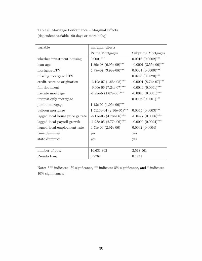
Table 8. Mortgage Performance —Marginal Effects
(dependent variable: 90-days or more deliq)
variable marginal effects
Prime Mortgages Subprime Mortgages
whether investment housing 0.0001∗∗∗ 0.0016 (0.0002)∗∗∗
loan age 1.39e-08 (6.95e-09)∗∗∗ -0.0001 (3.55e-06)∗∗∗
mortgage LTV 5.75e-07 (3.92e-08)∗∗∗ 0.0004 (0.0000)∗∗∗
missing mortgage LTV 0.0296 (0.0020)∗∗∗
credit score at origination -3.19e-07 (1.85e-08)∗∗∗ -0.0001 (8.74e-07)∗∗∗
full document -9.00e-06 (7.24e-07)∗∗∗ -0.0044 (0.0001)∗∗∗
fix-rate mortgage -1.99e-5 (1.67e-06)∗∗∗ -0.0046 (0.0001)∗∗∗
interest-only mortgage 0.0006 (0.0001)∗∗∗
jumbo mortgage 1.43e-06 (1.05e-06)∗∗∗
balloon mortgage 1.5113e-04 (2.36e-05)∗∗∗ 0.0045 (0.0003)∗∗∗
lagged local house price gr rate -6.17e-05 (4.73e-06)∗∗∗ -0.0477 (0.0006)∗∗∗
lagged local payroll growth -1.23e-05 (2.77e-06)∗∗∗ -0.0009 (0.0004)∗∗∗
lagged local employment rate 4.51e-06 (2.97e-06) 0.0002 (0.0004)
time dummies yes yes
state dummies yes yes
number of obs. 16,631,802 2,518,561
Pseudo R-sq 0.2767 0.1241
Note: *** indicates 1% signficance, ** indicates 5% significance, and * indicates
10% significance.
30
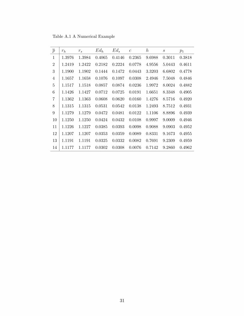
Table A.1 A Numerical Example
p rh rs Edh Eds c h s p1
1 1.3976 1.3984 0.4065 0.4146 0.2365 9.6988 0.3011 0.3818
2 1.2419 1.2422 0.2182 0.2224 0.0778 4.9556 5.0443 0.4611
3 1.1900 1.1902 0.1444 0.1472 0.0443 3.3203 6.6802 0.4778
4 1.1657 1.1658 0.1076 0.1097 0.0308 2.4946 7.5048 0.4846
5 1.1517 1.1518 0.0857 0.0874 0.0236 1.9972 8.0024 0.4882
6 1.1426 1.1427 0.0712 0.0725 0.0191 1.6651 8.3348 0.4905
7 1.1362 1.1363 0.0608 0.0620 0.0160 1.4276 8.5716 0.4920
8 1.1315 1.1315 0.0531 0.0542 0.0138 1.2493 8.7512 0.4931
9 1.1279 1.1279 0.0472 0.0481 0.0122 1.1106 8.8896 0.4939
10 1.1250 1.1250 0.0424 0.0432 0.0108 0.9997 9.0009 0.4946
11 1.1226 1.1227 0.0385 0.0393 0.0098 0.9088 9.0903 0.4952
12 1.1207 1.1207 0.0353 0.0359 0.0089 0.8331 9.1673 0.4955
13 1.1191 1.1191 0.0325 0.0332 0.0082 0.7691 9.2309 0.4959
14 1.1177 1.1177 0.0302 0.0308 0.0076 0.7142 9.2860 0.4962
31
100
120
140
160
180
200
hous
e pr
ice
inde
x (C
orel
ogic
)
.06
.08
.1.1
2.1
4.1
6sh
are
of in
vest
men
t hom
e ap
plic
atio
ns (%
)
Jan2000 Jan2002 Jan2004 Jan2006 Jan2008 Jan2010time
mortgage application # mortgage application $house price index (right axis)
Figure 1. Share of Investment Home Mortgage Applications and House Price Index —
US
.05
.1.1
5.2
.25
.3
Jan2000 Jan2002 Jan2004 Jan2006 Jan2008 Jan2010time
US AZCA FLNV
Source: HMDA
Figure 2. Share of Investment Housing Application Numbers —US and Selected States
32
02
46
8101
214
Den
sity
0 .2 .4 .6 .8 1year 2000
02
46
8101
214
Den
sity
0 .2 .4 .6 .8 1year 2005
02
46
8101
214
Den
sity
0 .2 .4 .6 .8 1year 2010
Figure 3. Histograms of Shares of Investment Housing Mortgage Applications
33
0.00
0.05
0.10
0.15
0.20
0.25
shar
e of
sub
prim
e m
ortg
age
apps
(%)
Jan2000 Jan2002 Jan2004 Dec2005time
of investment apps of all apps
Source: HMDA0.
000.
050.
100.
150.
200.
25sh
are
of in
vest
men
t mor
tgag
e ap
ps (%
)
Jan2000 Jan2002 Jan2004 Dec2005time
of subprime apps of all apps
Source: HMDA
Figure 4. Investment Housing and Subprime Mortgages (HMDA)
0.0
5.1
.15
.2.2
5.3
shar
e(%
)
200001 200201 200401 200601 200801 201001 201111time
Investment Homes Second Homes
Source: LPS
0.0
5.1
.15
.2.2
5.3
shar
e(%
)
200001 200201 200401 200601 200708time
Investment in Sub 2nd in SubInvestment in AltA 2nd in AltA
Source: Corelogic
Figure 5. Investment Mortgage Shares of Prime Mortgages and Subprime Mortgages
(LPS and Corelogic)
34