three essays on the elicitation of...
TRANSCRIPT
1
THREE ESSAYS ON THE ELICITATION OF WILLINGNESS-TO-PAY
By
LIJIA SHI
A DISSERTATION PRESENTED TO THE GRADUATE SCHOOL OF THE UNIVERSITY OF FLORIDA IN PARTIAL FULFILLMENT
OF THE REQUIREMENTS FOR THE DEGREE OF DOCTOR OF PHILOSOPHY
UNIVERSITY OF FLORIDA
2012

2
© 2012 Lijia Shi

3
To my parents

4
ACKNOWLEDGMENTS
I would like to express my gratitude to my committee members: Dr. Lisa A. House,
Dr. Zhifeng Gao, Dr. Kim Morgan and Dr. Chunrong Ai for their generous help and
support in the completion of this dissertation.
Most gratefully, I thank Dr. Lisa House and Dr. Zhifeng Gao for their generous help
and continuous encouragement. They have been among the best mentors in the
department and all my achievement during the last four years would not be possible
without their support.
Moreover, I want to thank Dr. Kim Morgan and Dr. Chunrong Ai for their valuable
comments and suggestions. They are both respected professionals. I believe their help
will also benefit me in my future studies.
I would also appreciate the support from my fellow graduate students. They made
my graduate life full of wonderful memories.
Last but not least, I would like to take this opportunity to thank my family,
especially my parents for their endless supports and love. Without them, my study
would not be possible.
5
TABLE OF CONTENTS page
ACKNOWLEDGMENTS .................................................................................................. 4
LIST OF TABLES ............................................................................................................ 7
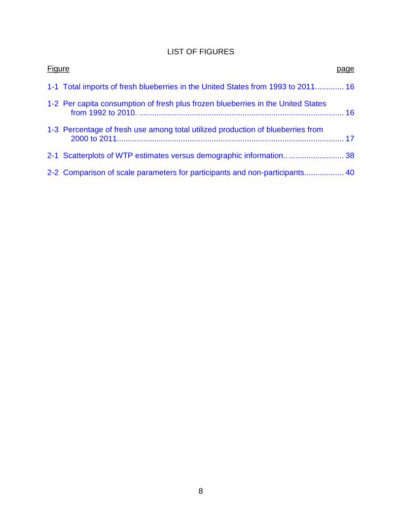
LIST OF FIGURES .......................................................................................................... 8
LIST OF ABBREVIATIONS ............................................................................................. 9
ABSTRACT ................................................................................................................... 10
CHAPTER
1 INTRODUCTION .................................................................................................... 12
1.1 Blueberry Market Review .............................................................................. 12 1.2 Consumer Willingness-to-Pay for Fruit Attributes ......................................... 13 1.3 Value Elicitation Method ............................................................................... 14
2 CONSUMER WILLINGNESS-TO-PAY FOR BLUEBERRY ATTRIBUTES: A HIERARCHICAL BAYESIAN APPROACH IN THE WILLINGNESS-TO-PAY SPACE .................................................................................................................... 18
2.1 Introduction ................................................................................................... 18 2.2 Consumer Attitudes for Food Attributes ........................................................ 21 2.3 The Choice Experiment and the Data ........................................................... 22 2.4 The Model ..................................................................................................... 24 2.5 Results .......................................................................................................... 26
2.5.1 Mixed Logit Estimation Result .............................................................. 27 2.5.2 Consumers’ WTPs for Blueberry Attributes .......................................... 27 2.5.3 The Reliability of the Individual-Level Estimates .................................. 30 2.5.4 Willingness-to-pay and Demographics ................................................. 31
2.6 Conclusion and Discussion ........................................................................... 31
3 ON MODEL SPECIFICATION OF THE MIXED LOGIT: THE CASE OF CONSUMER PERCEPTION ON BLUEBERRY ATTRIBUTES .............................. 41
3.1 Introduction ................................................................................................... 41 3.2 The Model ..................................................................................................... 45 3.3 Case Study: Consumer Preference for Blueberry Attributes ......................... 48 3.4 Results .......................................................................................................... 50 3.5 Conclusion and Discussion ........................................................................... 53
6
4 CONSUMERS’ WILLINGNESS-TO-PAY FOR ORGANIC AND LOCAL BLUEBERRIES: A MULTI-STORE BDM AUCTION CONTROLLING FOR PURCHASE INTENTIONS ..................................................................................... 58
4.1 Introduction ................................................................................................... 58 4.2 Literature Review .......................................................................................... 61 4.3 Auction Procedure ........................................................................................ 64 4.4 Results .......................................................................................................... 65
4.4.1 Partial Bids for Organic and Local Blueberries at Different Marketing Outlets ........................................................................................................... 66
4.4.2 Impact of Purchase Intention ................................................................ 67 4.4.3 The Tobit Model for Full Bids ................................................................ 68 4.4.4 The OLS Regression for Partial Bids .................................................... 70
4.5 Conclusion .................................................................................................... 71
5 CONCLUSION ........................................................................................................ 77
APPENDIX
A CHOICE SITUATIONS FOR THE CHOICE EXPERIMENT .................................... 81
B BDM AUCTION QUESTIONNAIRE ........................................................................ 84
C BDM AUCTION INSTRUCTIONS AND PROCEDURE........................................... 89
LIST OF REFERENCES ............................................................................................... 91
BIOGRAPHICAL SKETCH ............................................................................................ 98
7
LIST OF TABLES
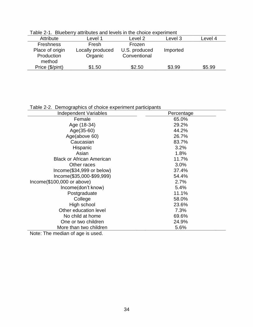
Table page 2-1 Blueberry attributes and levels in the choice experiment ....................................... 34
2-2 Demographics of choice experiment participants ................................................... 34
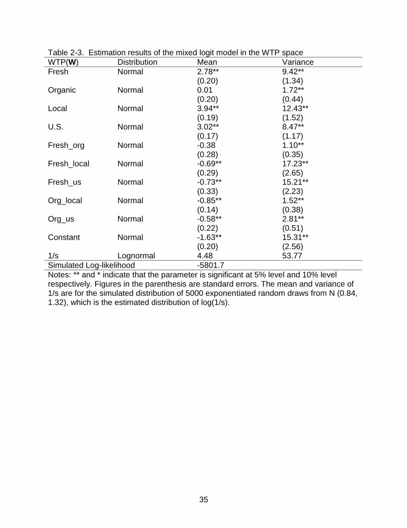
2-3 Estimation results of the mixed logit model in the WTP space ............................... 35
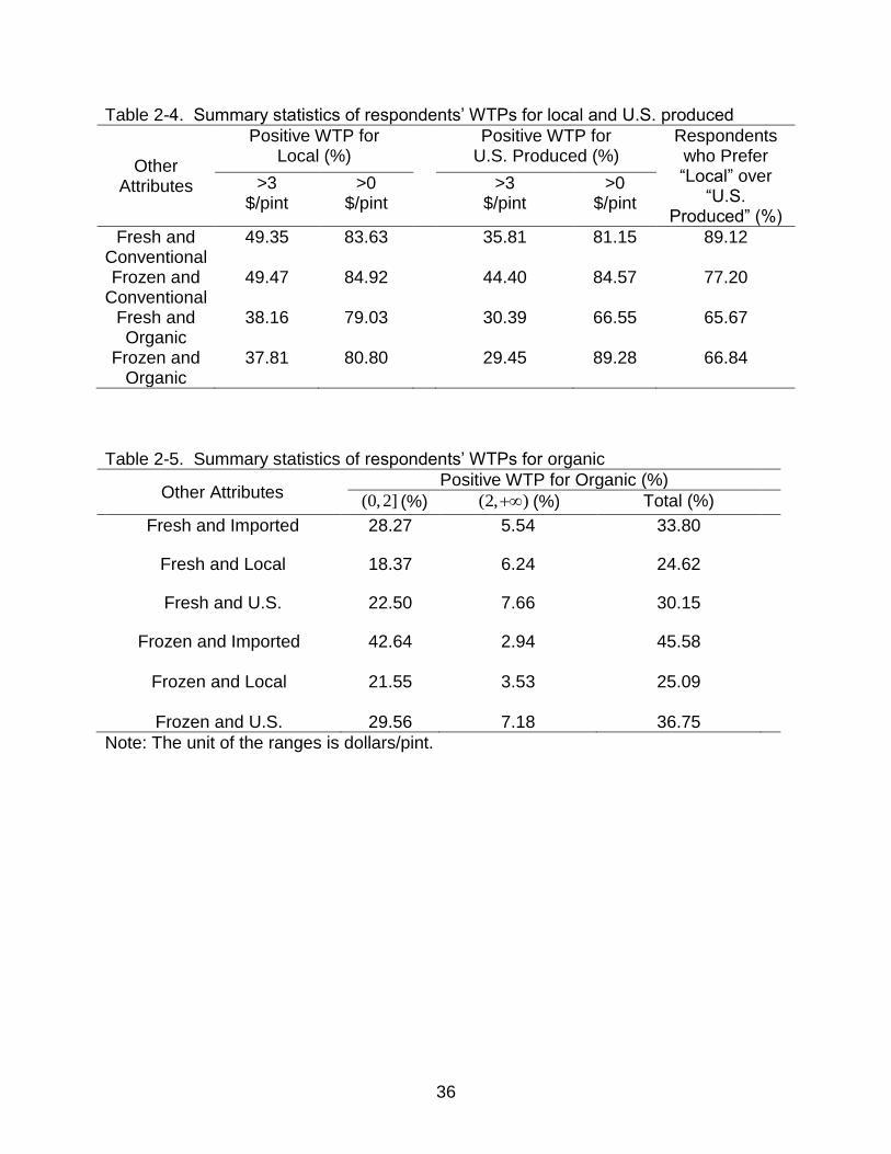
2-4 Summary statistics of respondents’ WTPs for local and U.S. produced ................. 36
2-5 Summary statistics of respondents’ WTPs for organic ........................................... 36
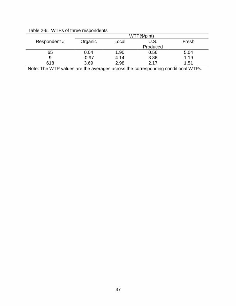
2-6 WTPs of three respondents ................................................................................... 37
3-1 Literature comparing models from preference space and WTP space ................... 55
3-2 Blueberry attributes and levels in the stated preference experiment ...................... 56
3-3 Estimation results of the three models ................................................................... 56
3-4 Means and variances of the individual-level WTP estimates ................................. 57
3-5 Correlation between individual-level WTP estimates among the three models. ..... 57
4-1 Demographics of participants at each marketing outlet .......................................... 73
4-2 Summary statistics of bids ..................................................................................... 73
4-3 Difference of mean bids across purchase intentions .............................................. 74
4-4 WTPs at different locations .................................................................................... 74
4-5 Tobit for reported bids ............................................................................................ 75
4-6 Robust OLS for WTPs ............................................................................................ 76
8
LIST OF FIGURES
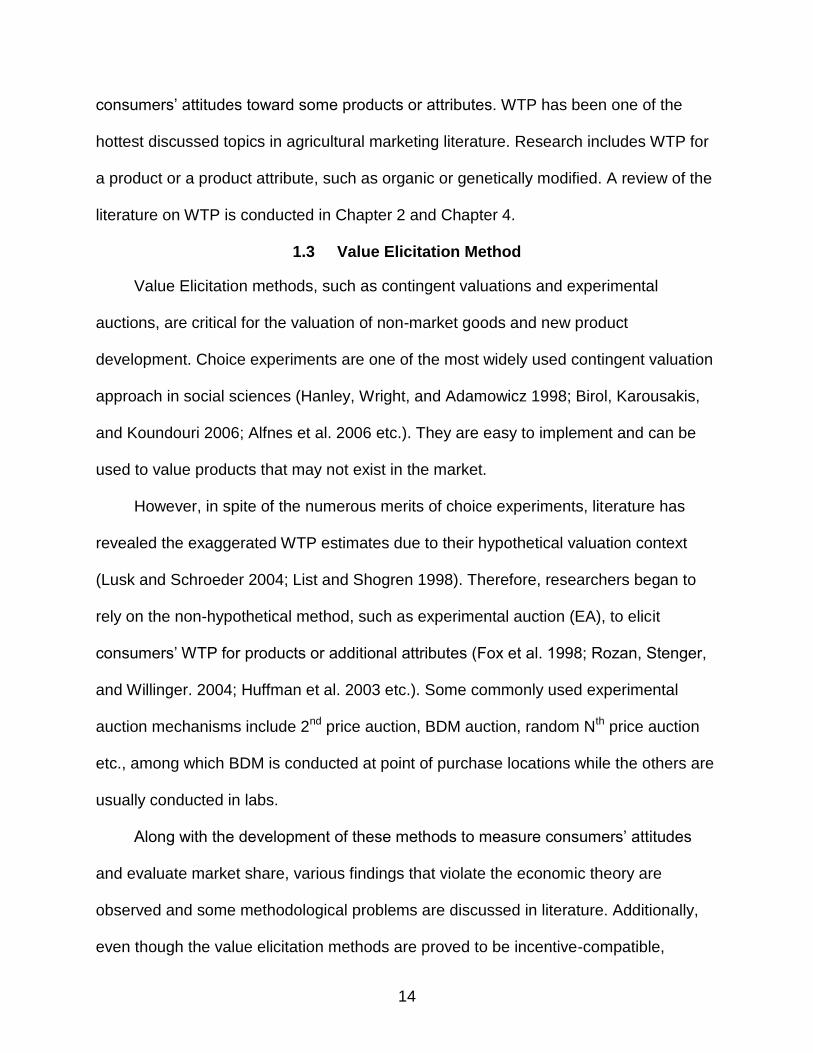
Figure page 1-1 Total imports of fresh blueberries in the United States from 1993 to 2011. ............ 16
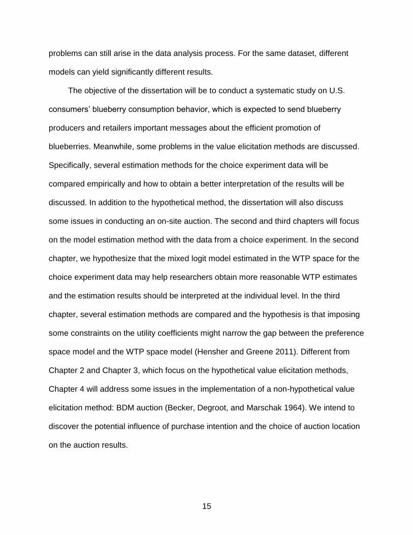
1-2 Per capita consumption of fresh plus frozen blueberries in the United States from 1992 to 2010. ............................................................................................. 16
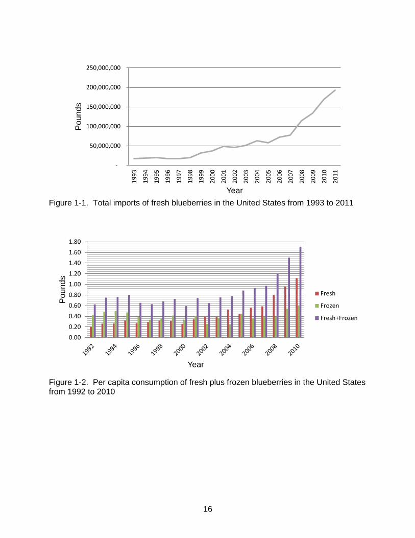
1-3 Percentage of fresh use among total utilized production of blueberries from 2000 to 2011....................................................................................................... 17
2-1 Scatterplots of WTP estimates versus demographic information.. ......................... 38
2-2 Comparison of scale parameters for participants and non-participants. ................. 40

9
LIST OF ABBREVIATIONS
HB Hierarchical Bayesian
WTP Willingness-to-pay

10
Abstract of Dissertation Presented to the Graduate School of the University of Florida in Partial Fulfillment of the Requirements for the Degree of Doctor of Philosophy
THREE ESSAYS ON THE ELICITATION OF WILLINGNESS-TO-PAY
By
Lijia Shi
August 2012
Chair: Lisa A. House Cochair: Zhifeng Gao Major: Food and Resource Economics
An online survey was designed to explore consumers’ blueberry consumption
behavior. A large amount of information is collected, including consumption habits,
attitudes and demographics. A choice experiment designed to elicit consumers’
willingness-to-pay (WTP) for several blueberry attributes was also included in the
survey. Additionally, a non-hypothetical method: experimental auction was conducted to
measure consumers’ WTP for organic and local blueberries. This dissertation used the
data from the two value elicitation methods: choice experiment and experimental
auction for empirical model comparisons and studies of consumer behavior.
In the first essay, a stated preference experiment is conducted to elicit consumers’
WTP for various blueberry attributes. A mixed logit model estimated by the hierarchical
Bayesian approach (HB) is employed to account for consumer heterogeneity and the
distributions of WTPs are directly specified. The results show that locally produced
blueberries are preferred over U.S. produced blueberries by most respondents. By
contrast, less than 50 percent of the respondents demonstrate positive premiums for
organic blueberries. Additionally, hardly any relationship between demographics and
WTPs is detected.
11
In the second essay, three specifications of the mixed logit model are compared.
The first is specified in the preference space with all parameters random. The second is
specified in the preference space with the coefficient of price fixed. The third is specified
in the WTP space with all parameters random. The data is from the choice experiment
eliciting consumers’ perception of several blueberry attributes: freshness, local and
organic. The purpose is to see whether fixing the price coefficient in the preference
space can narrow down the gap (i.e., difference in model fits and estimated coefficients)
between the preference space model and the WTP space model and how such
constraint affects the individual-level WTP estimates.
The third paper discusses consumers’ bidding behavior in the BDM auctions. The
impact of consumers’ purchase intention on their bidding behavior is investigated.
Additionally, the auction was conducted at multiple types of stores to capture a more
representative sample of consumers.
12
CHAPTER 1 INTRODUCTION
1.1 Blueberry Market Review
Blueberry is widely known as a healthy fruit. The consumption of blueberries has
experienced a dramatic change during the last few decades in the United States. In the
late 1990s, scientific research revealed special health benefits of blueberries. According
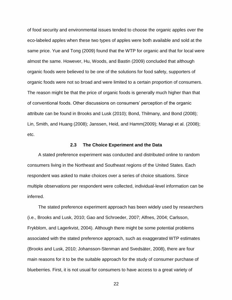
to the USDA, the total imports of fresh blueberries increased from 17.5 million pounds in
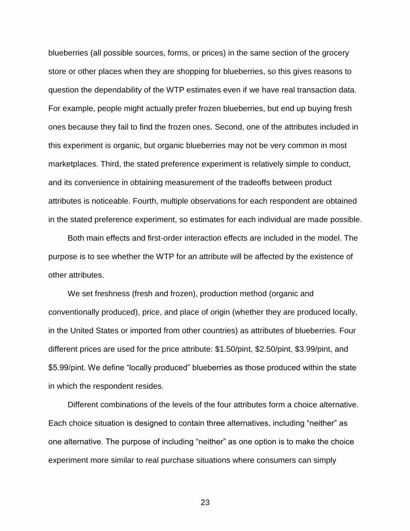
1993 to 192.5 million pounds in 2008 (Figure 1-1). At the same time, per capita
consumption of fresh and frozen blueberries in the U.S. increased (Figure 1-2), from
0.62 pounds in 1992 to 1.71 pounds in 2010 (USDA, Economics, Statistics, and Market
Information System). We can see that per capita consumption of fresh blueberries has
been increasing dramatically since 2000, but that of frozen blueberries has not
demonstrated any obvious increasing trend since 1992. While per capita consumption
of frozen blueberries is greater than that of fresh ones during the 1990’s, the
consumption of fresh blueberries has been dominating the non-processed blueberry
market since 2002.
It’s projected that per capita consumption level of blueberries in the United States
can reach 44 ounces by 2015 (U.S. Highbush Blueberry Council). In spite of the overall
growing consumption level, there is still quite large undeveloped domestic market.
Consumption may be further motivated by the education of the health benefits of
blueberries among consumers and effective promotion strategies. As a leading
blueberry producer in the world, the blueberry segment in the United States will
encounter thriving commercial opportunities with the expanding national consumption
level. At this critical time of development, retailers should set up corresponding
13
promotion plan based on a comprehensive understanding of the structure of blueberry
market.
The quantity of literature on the consumption of blueberries is quite limited,
especially on the consumption of non-processed (fresh+ frozen) blueberries. To our
knowledge, the only literature on consumer preference for blueberries is from Hu,
Woods, and Bastin (2009), which focused on processed blueberry products. According
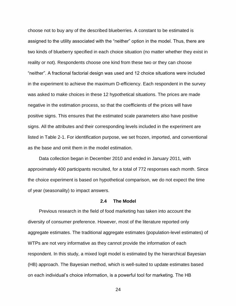
to the data from USDA, the percentage of the fresh use among total utilized production
of blueberries increased from 27.1% in 2000 to 54.6% in 2011 (Figure 1-3). The
percentage is expected to keep rising as more people have realized the health benefits
of blueberries. Also, non-processed blueberries usually possess higher market values
and consumer acceptance. Therefore, we will conduct a systematic study about the
consumption behavior of non-processed blueberries, such as how do consumers
tradeoff different blueberry attributes and how much they would pay for the credence
attributes like organic. Our results will serve as reference for the setup of effective
marketing strategies, which is crucial for potential expanding of the blueberry market.
1.2 Consumer Willingness-to-Pay for Fruit Attributes
With the rising concern about health and environment among consumers, the
production method or production location of food has received plenty of attention.
Researchers have come up with various methods to elicit consumers’ willingness-to-pay
(WTP) for value-added food attributes, such as organic and local. In economics, WTP is
known as the maximum amount of money people would be willing to pay for a good or
an attribute. Different from people’s attitude or perception, which cannot be quantified,
WTP can be measured with some economic methods (i.e. choice experiment or
experimental auctions). Thus, WTP enables researchers to quantify and compare
14
consumers’ attitudes toward some products or attributes. WTP has been one of the
hottest discussed topics in agricultural marketing literature. Research includes WTP for
a product or a product attribute, such as organic or genetically modified. A review of the
literature on WTP is conducted in Chapter 2 and Chapter 4.
1.3 Value Elicitation Method
Value Elicitation methods, such as contingent valuations and experimental
auctions, are critical for the valuation of non-market goods and new product
development. Choice experiments are one of the most widely used contingent valuation
approach in social sciences (Hanley, Wright, and Adamowicz 1998; Birol, Karousakis,
and Koundouri 2006; Alfnes et al. 2006 etc.). They are easy to implement and can be
used to value products that may not exist in the market.
However, in spite of the numerous merits of choice experiments, literature has
revealed the exaggerated WTP estimates due to their hypothetical valuation context
(Lusk and Schroeder 2004; List and Shogren 1998). Therefore, researchers began to
rely on the non-hypothetical method, such as experimental auction (EA), to elicit
consumers’ WTP for products or additional attributes (Fox et al. 1998; Rozan, Stenger,
and Willinger. 2004; Huffman et al. 2003 etc.). Some commonly used experimental
auction mechanisms include 2nd price auction, BDM auction, random Nth price auction
etc., among which BDM is conducted at point of purchase locations while the others are
usually conducted in labs.
Along with the development of these methods to measure consumers’ attitudes
and evaluate market share, various findings that violate the economic theory are
observed and some methodological problems are discussed in literature. Additionally,
even though the value elicitation methods are proved to be incentive-compatible,
15
problems can still arise in the data analysis process. For the same dataset, different
models can yield significantly different results.
The objective of the dissertation will be to conduct a systematic study on U.S.
consumers’ blueberry consumption behavior, which is expected to send blueberry
producers and retailers important messages about the efficient promotion of
blueberries. Meanwhile, some problems in the value elicitation methods are discussed.
Specifically, several estimation methods for the choice experiment data will be
compared empirically and how to obtain a better interpretation of the results will be
discussed. In addition to the hypothetical method, the dissertation will also discuss
some issues in conducting an on-site auction. The second and third chapters will focus
on the model estimation method with the data from a choice experiment. In the second
chapter, we hypothesize that the mixed logit model estimated in the WTP space for the
choice experiment data may help researchers obtain more reasonable WTP estimates
and the estimation results should be interpreted at the individual level. In the third
chapter, several estimation methods are compared and the hypothesis is that imposing
some constraints on the utility coefficients might narrow the gap between the preference
space model and the WTP space model (Hensher and Greene 2011). Different from
Chapter 2 and Chapter 3, which focus on the hypothetical value elicitation methods,
Chapter 4 will address some issues in the implementation of a non-hypothetical value
elicitation method: BDM auction (Becker, Degroot, and Marschak 1964). We intend to
discover the potential influence of purchase intention and the choice of auction location
on the auction results.
16
Figure 1-1. Total imports of fresh blueberries in the United States from 1993 to 2011
Figure 1-2. Per capita consumption of fresh plus frozen blueberries in the United States from 1992 to 2010
-
50,000,000
100,000,000
150,000,000
200,000,000
250,000,000
19
93
19
94
19
95
19
96
19
97
19
98
19
99
20
00
20
01
20
02
20
03
20
04
20
05
20
06
20
07
20
08
20
09
20
10
20
11
Po
un
ds
Year
0.00
0.20
0.40
0.60
0.80
1.00
1.20
1.40
1.60
1.80
Po
un
ds
Year
Fresh
Frozen
Fresh+Frozen
17
Figure 1-3. Percentage of fresh use among total utilized production of blueberries from 2000 to 2011
0
0.1
0.2
0.3
0.4
0.5
0.6
2000 2001 2002 2003 2004 2005 2006 2007 2008 2009 2010 2011
Pe
rcen
tage
Year
18
CHAPTER 2 CONSUMER WILLINGNESS-TO-PAY FOR BLUEBERRY ATTRIBUTES: A
HIERARCHICAL BAYESIAN APPROACH IN THE WILLINGNESS-TO-PAY SPACE
2.1 Introduction
Per capita consumption of fresh blueberries has increased dramatically since 2000
(United States Department of Agriculture, Economic Research Service [USDA/ERS]).
This growth reflects both increased consumer awareness of the importance of healthy
diets and the proactive effort by the U.S. blueberry industry in publicizing the benefits
from blueberry consumption. Faced with such rapid growth of this new market, a
systematic study about consumer behavior in blueberry consumption is critical.
Consumer choice of fruit has become complicated, as even the same type of fruit,
for example, blueberries, can have multiple attributes. Market segmentation is used to
reach different consumer segments. In a market rapidly growing market such as the one
for blueberries, understanding consumer choice of these attribute combinations is
perhaps even more critical. Production method, origin of production, and form of the fruit
(i.e., frozen versus fresh) are among a number of attributes (appearance, flavor, price,
etc.) that consumers consider when purchasing fruit. Consumers’ choices depend highly
on their preferences. Some consumers may prefer fresh blueberries over frozen ones,
while other consumers may prefer frozen blueberries because of their long shelf-life. As
for the credence attributes, such as production method (i.e., organic) and production
location (country of origin), consumers’ perception also demonstrates large variance.
Some consumers may consider country of origin of blueberries a more important
attribute than whether the product is fresh or frozen, while to others, country of origin
may not be important. Some consumers prefer organic production and thus are willing
to pay more for organic blueberries. Though this preference choice has been shown to
19
exist for other fruits (i.e., Lin, Smith, and Huang, 2008; Batte et al., 2007; Yue and Tong,
2009; Loureiro, McCluskey, and Mittelhammer, 2001), it is important to explore the size
of the consumer segments specifically for blueberries. Different consumers appreciate
different attributes, thus, marketing strategies that fail to take consumer heterogeneity
into account are destined to be less efficient.
The explanatory power of demographics for consumption behavior is limited
(Frank, Massy, and Boyd, 1967; Yankelovich, 1964), especially for small purchases
such as one pint of blueberries in a highly competitive fruit market. This study will
compare the importance of different attributes on consumer willingness-to-pay (WTP)
for blueberries at the individual-level. If consumers have a diversity of opinions
regarding fruit attributes, especially given the large amount of substitutes in the fruit
market, a single marketing strategy might not be ideal. Studying the impact of attributes
on different consumers will aid blueberry producers to target different consumers with
different marketing strategies.
The objective of this study is to compare consumers’ attitudes toward four
blueberry attributes and differentiate consumers in terms of their individual-level WTP
estimates (i.e., WTP estimates for each respondent). Our work contributes to the
literature in two aspects. First, we examine consumers’ perception of the attributes of
non-processed (fresh) and frozen blueberries. To our knowledge, the literature on
blueberry consumption (Hu, Woods, and Bastin, 2009; Hu et al., 2011; etc.) mainly
focused on the attributes of processed blueberry products. Non-processed blueberries
possess much higher market values and consumer recognition. Additionally, the
percentage of fresh use among utilized production of blueberries increased from 27.1%
20
in 2000 to almost 54.6% in 2009 (USDA).1 The percentage is expected to keep rising as
more people realize the health benefits of fresh blueberries.
Second, our results are based on the individual-level estimates, which provide
valuable information about the variety of consumer attitudes, such as diversified
attribute importance ranking. Such information is extremely valuable when demographic
information is not available or the explanatory power of demographics is marginal. Most
previous literature reported only aggregate WTP estimates (i.e., the average WTP) or
the distribution of WTPs across consumers, which are much less informative for the
implementation of differential marketing. Individual-level estimates provide us with
valuable information about individual consumption behavior, which is indispensable for
differential marketing strategies. For example, price-cut strategies are expected to be
more effective for consumers who are more sensitive to price. Organic labeling may
only attract those who prefer organic production. In this light, supermarkets can issue
different types of coupons to different consumers based on their individual preferences
(Rossi, McCulloch, and Allenby, 1996). In addition, since all kinds of WTP elicitation
methods have some shortcomings, the accuracy of the WTP estimate cannot be
guaranteed. The comparison of the relative importance of various attributes might be of
more practical value. The individual-level estimates enable us to calculate the
proportion of consumers that prefer one attribute over another. Such information cannot
be obtained from the two estimated distributions of WTPs for the two attributes.
1 The number is based on the production and utilization data of Maine, Michigan, New Jersey, North
Carolina, Oregon, Washington, Alabama, Arkansas, Florida, Georgia, Indiana, New York, California and Mississippi.
21
2.2 Consumer Attitudes for Food Attributes
There is a large amount of literature on the valuation of food attributes. For
example, country of origin is among the most popularly discussed food attributes in
recent years and is an important characteristic in consumers’ purchasing decisions.
Umberger et al. (2003) showed that most consumers were willing to pay premiums for
the “USA Guaranteed” label on steak. The food safety concerns and belief in higher
quality of U.S. products are generally believed to be one of the main reasons for
consumers’ recognition of U.S. products. In addition to the country of origin label, the
“locally grown” attribute of fruits or vegetables has been gaining popularity. Dentoni et
al. (2009) found that the attribute of “locally grown” directly affected consumers’
purchasing behavior for apples. In the study of Hu, Woods, and Bastin (2009),
consumers in Kentucky were found to demonstrate higher WTP for “locally produced
(within the state of Kentucky)” than for organic and sugar-free attributes of processed
blueberry products. Darby et al. (2006) also concluded that consumers were willing to
pay more for locally grown strawberries than for those just with “produced in the U.S.”
label.
In addition to country of origin, there is extensive literature on the choice between
organic and conventional products. Wang and Sun (2003) concluded that the organic
market had a large consumer base and it’s future was promising. Batte et al. (2007)
considered multi-ingredient processed organic foods with four levels of organic content
under the National Organic Program (100% organic, 95% organic, 70-95% organic,
<70%organic). Their results indicated that customers were willing to pay a premium for
food with organic content, even those that were not totally organic. Loureiro,
McCluskey, and Mittelhammer (2001) showed that consumers with similar perceptions
22
of food security and environmental issues tended to choose the organic apples over the
eco-labeled apples when these two types of apples were both available and sold at the
same price. Yue and Tong (2009) found that the WTP for organic and that for local were
almost the same. However, Hu, Woods, and Bastin (2009) concluded that although
organic foods were believed to be one of the solutions for food safety, supporters of
organic foods were not so broad and were limited to a certain proportion of consumers.
The reason might be that the price of organic foods is generally much higher than that
of conventional foods. Other discussions on consumers’ perception of the organic
attribute can be found in Brooks and Lusk (2010); Bond, Thilmany, and Bond (2008);
Lin, Smith, and Huang (2008); Janssen, Heid, and Hamm(2009); Managi et al. (2008);
etc.
2.3 The Choice Experiment and the Data
A stated preference experiment was conducted and distributed online to random
consumers living in the Northeast and Southeast regions of the United States. Each
respondent was asked to make choices over a series of choice situations. Since
multiple observations per respondent were collected, individual-level information can be
inferred.
The stated preference experiment approach has been widely used by researchers
(i.e., Brooks and Lusk, 2010; Gao and Schroeder, 2007; Alfnes, 2004; Carlsson,
Frykblom, and Lagerkvist, 2004). Although there might be some potential problems
associated with the stated preference approach, such as exaggerated WTP estimates
(Brooks and Lusk, 2010; Johansson-Stenman and Svedsäter, 2008), there are four
main reasons for it to be the suitable approach for the study of consumer purchase of
blueberries. First, it is not usual for consumers to have access to a great variety of
23
blueberries (all possible sources, forms, or prices) in the same section of the grocery
store or other places when they are shopping for blueberries, so this gives reasons to
question the dependability of the WTP estimates even if we have real transaction data.
For example, people might actually prefer frozen blueberries, but end up buying fresh
ones because they fail to find the frozen ones. Second, one of the attributes included in
this experiment is organic, but organic blueberries may not be very common in most
marketplaces. Third, the stated preference experiment is relatively simple to conduct,
and its convenience in obtaining measurement of the tradeoffs between product
attributes is noticeable. Fourth, multiple observations for each respondent are obtained
in the stated preference experiment, so estimates for each individual are made possible.
Both main effects and first-order interaction effects are included in the model. The
purpose is to see whether the WTP for an attribute will be affected by the existence of
other attributes.
We set freshness (fresh and frozen), production method (organic and
conventionally produced), price, and place of origin (whether they are produced locally,
in the United States or imported from other countries) as attributes of blueberries. Four
different prices are used for the price attribute: $1.50/pint, $2.50/pint, $3.99/pint, and
$5.99/pint. We define “locally produced” blueberries as those produced within the state
in which the respondent resides.
Different combinations of the levels of the four attributes form a choice alternative.
Each choice situation is designed to contain three alternatives, including “neither” as
one alternative. The purpose of including “neither” as one option is to make the choice
experiment more similar to real purchase situations where consumers can simply
24
choose not to buy any of the described blueberries. A constant to be estimated is
assigned to the utility associated with the “neither” option in the model. Thus, there are
two kinds of blueberry specified in each choice situation (no matter whether they exist in
reality or not). Respondents choose one kind from these two or they can choose
“neither”. A fractional factorial design was used and 12 choice situations were included
in the experiment to achieve the maximum D-efficiency. Each respondent in the survey
was asked to make choices in these 12 hypothetical situations. The prices are made
negative in the estimation process, so that the coefficients of the prices will have
positive signs. This ensures that the estimated scale parameters also have positive
signs. All the attributes and their corresponding levels included in the experiment are
listed in Table 2-1. For identification purpose, we set frozen, imported, and conventional
as the base and omit them in the model estimation.
Data collection began in December 2010 and ended in January 2011, with
approximately 400 participants recruited, for a total of 772 responses each month. Since
the choice experiment is based on hypothetical comparison, we do not expect the time
of year (seasonality) to impact answers.
2.4 The Model
Previous research in the field of food marketing has taken into account the
diversity of consumer preference. However, most of the literature reported only
aggregate estimates. The traditional aggregate estimates (population-level estimates) of
WTPs are not very informative as they cannot provide the information of each
respondent. In this study, a mixed logit model is estimated by the hierarchical Bayesian
(HB) approach. The Bayesian method, which is well-suited to update estimates based
on each individual’s choice information, is a powerful tool for marketing. The HB
25
approach also has irreplaceable advantages in finite sample inference (Rossi, Allenby,
and McCulloch, 2005) and can generate the individual-level estimates as byproducts
(Allenby and Rossi, 1998). To obtain more sensible and accurate WTP estimates, we
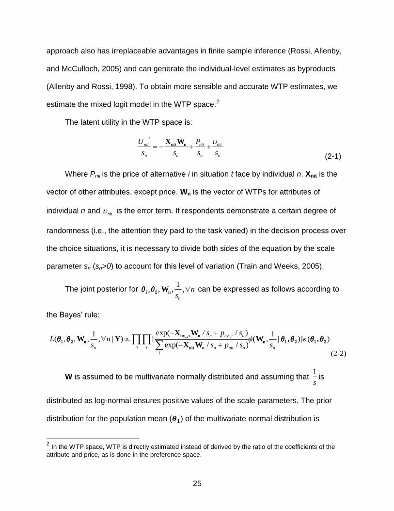
estimate the mixed logit model in the WTP space.2
The latent utility in the WTP space is:
'
nit nit nit
n n n n
U P
s s s s
nit nX W
(2-1)
Where Pnit is the price of alternative i in situation t face by individual n. Xnit is the
vector of other attributes, except price. Wn is the vector of WTPs for attributes of
individual n and nit is the error term. If respondents demonstrate a certain degree of
randomness (i.e., the attention they paid to the task varied) in the decision process over
the choice situations, it is necessary to divide both sides of the equation by the scale
parameter sn (sn>0) to account for this level of variation (Train and Weeks, 2005).
The joint posterior for 1
, , , ,n
ns
nW1 2θθ can be expressed as follows according to
the Bayes’ rule:
exp( / / )1 1
( , , , , | ) [ ( , | )] ( )exp( / / )
ntn ny t n
n tn n nit n n
i
s p sL n
s s p s s
ntny t n
n n
nit n
X WW Y W
X W1 2 1 2 1 2θθ θ,θ θ,θ
(2-2)
W is assumed to be multivariate normally distributed and assuming that is
distributed as log-normal ensures positive values of the scale parameters. The prior
distribution for the population mean ( ) of the multivariate normal distribution is
2 In the WTP space, WTP is directly estimated instead of derived by the ratio of the coefficients of the
attribute and price, as is done in the preference space.
1
s
26
assumed to be diffuse multivariate normal, and that for the population variance ( ) is
assumed diffuse inverted Wishart. Nonzero covariance is allowed between the elements
of W and .
The HB approach relies on the Gibbs sampler to obtain the draws of1
,ns
nW , based
on which population-level parameter estimates are calculated. Thirty thousand iterations
are taken during the burn-in period (before convergence) and 5,000 every other tenth
draw3 are retained after burn-in to calculate the parameter estimates. Detail of the
Gibbs sampler can be found in Robert and Casella (2004) or Casella and George
(1992). The HB method is used because it gives out the individual-level estimates as
byproducts, so no additional procedures are needed (Allenby and Rossi, 1998). Details
of the Bayesian method can be found in Rossi, Allenby, and McCulloch (2005) and
Train (2003).
2.5 Results
Table 2-2 lists the demographic information of the choice experiment respondents.
Among the respondents, 65.0% of them are females. The average age is approximately
47 and the average household income is about $53,403 approximately. 83.7% of the
respondents are Caucasian, 3.2% are Hispanic and 11.7% are Black, or African
American. The rest are Asian, American Indian, native Hawaiian or Pacific Islander, etc.
23.6% of the respondents have a high school degree or equivalent, 58.0% have a four-
year college degree or some college, and 11.1% have attained a postgraduate degree.
3 In this way, correlation between subsequent retained draws can be reduced.
1
s
27
69.6% of the respondents don’t have children at home and 24.9% of them have one or
two children.
2.5.1 Mixed Logit Estimation Result
The estimation results of the mixed logit model are presented in Table 2-3. Most of
the estimated population means of the WTPs are significant at the 5% level. The
variances of the WTP distributions of all attributes are significantly different from zero at
the 5% level. Thus, we conclude that consumer heterogeneity does exist. The estimated
population means of the WTPs are significantly positive for fresh, locally produced, and
U.S. produced. This is consistent with our expectation that U.S. consumers generally
pay more for fresh blueberries than for frozen ones and pay more for local and U.S.
blueberries than for imported ones. However, the mean WTP estimate of organic is not
significantly different from zero, which indicates that consumers in general might be
indifferent about whether the blueberries are organic or not.
The estimated means for all interaction terms are negative and are significant
except for the interaction between fresh and organic. The negative signs of the
interaction terms can be explained as the outcome of the concavity of the utility function.
2.5.2 Consumers’ WTPs for Blueberry Attributes
The proportions of respondents who fall in a certain range of WTP values for each
attribute are shown in Tables 2-4 and Table 2-5. This method of summarizing individual-
level WTPs is used because of its robustness to extreme values.
The comparison of estimated WTPs for local and U.S. produced blueberries are
shown in Table 2-4. While the proportions of positive WTPs for local and U.S. produced
do not show much difference, the proportions of WTP estimates above $3/pint are all
bigger for local than for U.S. produced. These figures indicate that most U.S.
28
consumers hold the identical attitude that U.S produced blueberries are superior to
imported ones and, at the same time, some consumers are willing to pay more for local
than for simply U.S. produced. The last column of Table 2-4 lists the percentage of
respondents whose WTPs for local are bigger than that for U.S. produced. All of the
percentages exceed 65.7%, with the largest reaching nearly 89.1%. Therefore, the
majority of the respondents prefer local over simply U.S produced blueberries. We
conclude that locally produced blueberries can attract a larger price premium than
simply U.S. produced blueberries. This is also indicated by the larger population mean
of Wlocal compared to WU.S. in Table 2-3.
Although the population mean of Worg (Table 2-3) is not significantly different from
zero, 24.6% to 45.6% of the respondents are willing to pay a positive premium for
organic blueberries, depending on the other attributes (Table 2-5). The largest
proportion (45.6%) is for frozen and imported blueberries. Thus, the organic blueberries
are most attractive when the other favorable blueberry attributes (fresh and U.S.
produced) are not available. Although a certain proportion of respondents are
demonstrating positive WTPs for organic attribute, only a small proportion are willing to
pay more than $2/pint.
In addition to the stated preference questions, participants answered questions
designed to elicit their attitudes towards organic fruits and vegetables. Only 51.9% of
the respondents agreed or strongly agreed to the statement of “I trust fruits and
vegetables labeled as organic” and only 28.8% of the respondents agreed or strongly
agreed to the statement of “I will pay more for fruits and vegetables with an organic
label.” Therefore, it is not surprising that there are a relatively low proportion of positive
29
WTPs for organic. The result from the stated preference experiment is consistent with
the result from the attitude statement questions. Based on the average WTP for each
attribute across the other attribute combinations, we find that 95.1% of the respondents
are willing to pay more for U.S. produced blueberries than for organic ones and the
proportion is 96.4% when we compare local and organic blueberries. Thus, the results
indicate that consumers place more emphasis on the country of origin attribute than
they do on organic.
One finding from the Bayesian estimates worth attention is that there are a large
proportion of negative individual-level WTP estimates for organic. One of the reasons
might be the assumption of normal distribution for W, which does not impose any
restrictions on the signs of the WTP estimates. The other reason might be that some
respondents ignored the attribute of organic because of indifference, especially when
they saw other more favorable attributes in the choice sets. Therefore, we might
interpret the result as the outcome of a simplified mechanism behind respondents’
judgments in the choice experiment.
A final example of the individual differences found is shown in Table 2-6. WTP
values of three respondents (numbers 9, 65, and 618) are shown. In this case, the
differences among the participants are clearly seen. For example, participant 65 is
willing to pay more for fresh blueberries and respondent 618 is willing to pay more for
organic blueberries, while respondent 9 places the highest value on the country of origin
attribute. From this simple illustration, differences among consumers and the weights
they place on each attribute are demonstrated. Although the average WTP for organic
30
blueberries across all the respondents is nearly zero, there are still respondents who
demonstrate substantial positive WTPs for organic blueberries.
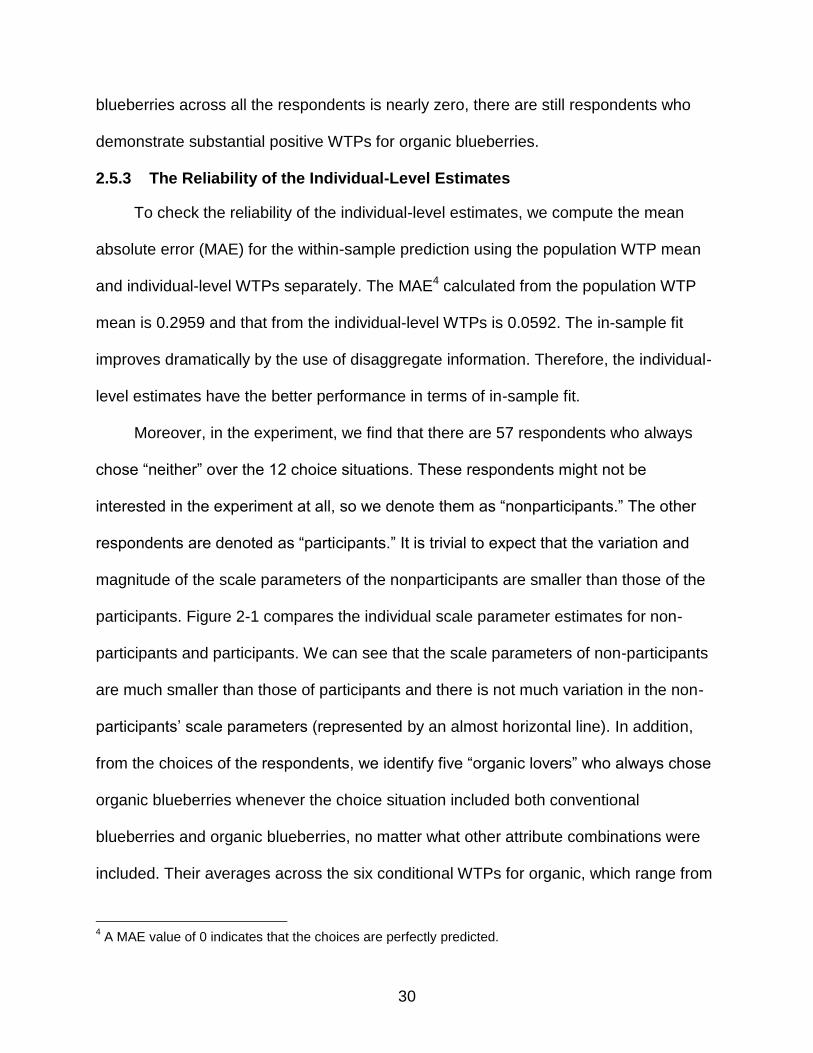
2.5.3 The Reliability of the Individual-Level Estimates
To check the reliability of the individual-level estimates, we compute the mean
absolute error (MAE) for the within-sample prediction using the population WTP mean
and individual-level WTPs separately. The MAE4 calculated from the population WTP
mean is 0.2959 and that from the individual-level WTPs is 0.0592. The in-sample fit
improves dramatically by the use of disaggregate information. Therefore, the individual-
level estimates have the better performance in terms of in-sample fit.
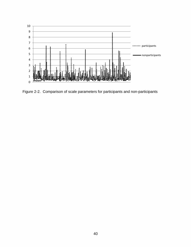
Moreover, in the experiment, we find that there are 57 respondents who always
chose “neither” over the 12 choice situations. These respondents might not be
interested in the experiment at all, so we denote them as “nonparticipants.” The other
respondents are denoted as “participants.” It is trivial to expect that the variation and
magnitude of the scale parameters of the nonparticipants are smaller than those of the
participants. Figure 2-1 compares the individual scale parameter estimates for non-
participants and participants. We can see that the scale parameters of non-participants
are much smaller than those of participants and there is not much variation in the non-
participants’ scale parameters (represented by an almost horizontal line). In addition,
from the choices of the respondents, we identify five “organic lovers” who always chose
organic blueberries whenever the choice situation included both conventional
blueberries and organic blueberries, no matter what other attribute combinations were
included. Their averages across the six conditional WTPs for organic, which range from
4 A MAE value of 0 indicates that the choices are perfectly predicted.
31
$3.69/pint to $4.00/pint, are also the biggest among all the respondents. Therefore,
although the number of observations for each respondent is not big enough (t=12), the
updated Bayesian individual-level estimates are fairly informative.
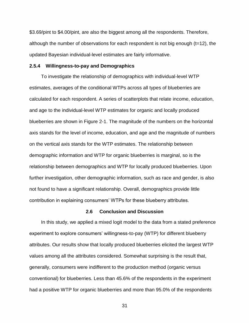
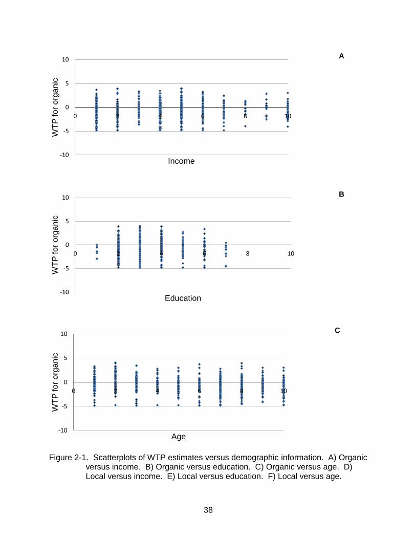
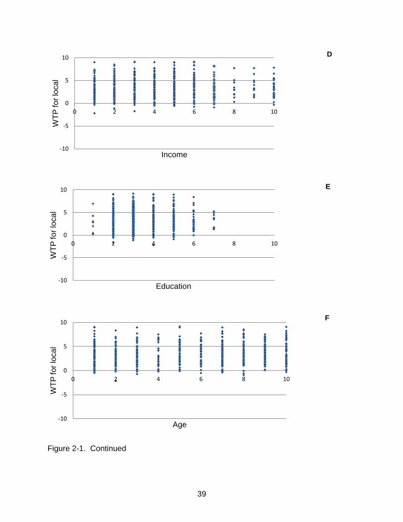
2.5.4 Willingness-to-pay and Demographics
To investigate the relationship of demographics with individual-level WTP
estimates, averages of the conditional WTPs across all types of blueberries are
calculated for each respondent. A series of scatterplots that relate income, education,
and age to the individual-level WTP estimates for organic and locally produced
blueberries are shown in Figure 2-1. The magnitude of the numbers on the horizontal
axis stands for the level of income, education, and age and the magnitude of numbers
on the vertical axis stands for the WTP estimates. The relationship between
demographic information and WTP for organic blueberries is marginal, so is the
relationship between demographics and WTP for locally produced blueberries. Upon
further investigation, other demographic information, such as race and gender, is also
not found to have a significant relationship. Overall, demographics provide little
contribution in explaining consumers’ WTPs for these blueberry attributes.
2.6 Conclusion and Discussion
In this study, we applied a mixed logit model to the data from a stated preference
experiment to explore consumers’ willingness-to-pay (WTP) for different blueberry
attributes. Our results show that locally produced blueberries elicited the largest WTP
values among all the attributes considered. Somewhat surprising is the result that,
generally, consumers were indifferent to the production method (organic versus
conventional) for blueberries. Less than 45.6% of the respondents in the experiment
had a positive WTP for organic blueberries and more than 95.0% of the respondents
32
placed more emphasis on the origin attribute than they did on organic. Though
potentially surprising when compared to other fruits, this result is supported by the
responses to the attitude statement questions. It can also be interpreted as the result of
a quickly growing market, in which consumers have not adapted fast enough to demand
organic blueberries yet. As a validation method, we estimated the model using
additional data (data from the same experiment but different sample of respondents)
and the results (i.e., overall ranking of the importance of attributes, estimated
parameters) are almost identical.
Consumer preferences and attitudes are highly diversified. The traditional method
of relying on demographic information to explain consumer behavior may not always be
effective, especially for small purchases like fruits or vegetables. While the purchases of
houses or cars might somehow reflect people’s economic or educational condition, the
choices of fruits might not be well differentiated by demographic characteristics. Our
results show that although there are big differences among respondents’ WTPs,
demographic information makes little contribution in explaining tradeoffs for blueberry
attributes.
The individual level WTP estimates provides us with valuable dis-aggregate
information that can help retailers differentiate consumers and set up more effective
marketing strategies. With the rapid growth in information technology, supermarkets can
issue different coupons or leaflets to different consumers based on their individual
attitudes instead of distributing them indiscriminately (Rossi, McCulloch, and Allenby,
1996). Coupons or brochures with sales featuring imported blueberries might only work
with consumers who do not have a strong bias toward imported fruits (i.e., respondent
33
65 if compared with the other two respondents in Table 2-6). Retailers can also issue
coupons of different values, depending on the price sensitivities of consumers. Such
differential promotion strategies can expand sales volume while increasing retailers’
profits. Moreover, consumer preference may not always be stable. The dynamic change
in consumer preference or perception can also be captured by Bayesian estimation.
There are several limitations of our study. First, our experiment was constrained
by the limited space of the survey and concern on respondent burn-out, so the number
of observations per respondent was not enough to make an unbiased estimation of the
individual-level WTP estimates, though the estimates already enabled us to compare
respondents’ valuation of blueberry attributes. Second, only within-sample prediction
criterion was used to compare the performances of individual-level estimates and
population-level estimates. Out-of-sample prediction should also be conducted for a
more comprehensive performance comparison.
34
Table 2-1. Blueberry attributes and levels in the choice experiment
Attribute Level 1 Level 2 Level 3 Level 4
Freshness Fresh Frozen Place of origin Locally produced U.S. produced Imported
Production method
Organic Conventional
Price ($/pint) $1.50 $2.50 $3.99 $5.99
Table 2-2. Demographics of choice experiment participants
Independent Variables Percentage
Female 65.0% Age (18-34) 29.2% Age(35-60) 44.2%
Age(above 60) 26.7% Caucasian 83.7% Hispanic 3.2%
Asian 1.8% Black or African American 11.7%
Other races 3.0% Income($34,999 or below) 37.4% Income($35,000-$99,999) 54.4%
Income($100,000 or above) 2.7% Income(don’t know) 5.4%
Postgraduate 11.1% College 58.0%
High school 23.6% Other education level 7.3%
No child at home 69.6% One or two children 24.9%
More than two children 5.6%
Note: The median of age is used.
35
Table 2-3. Estimation results of the mixed logit model in the WTP space
WTP(W) Distribution Mean Variance
Fresh
Normal 2.78** (0.20)
9.42** (1.34)
Organic Normal 0.01 (0.20)
1.72** (0.44)
Local Normal 3.94** (0.19)
12.43** (1.52)
U.S. Normal 3.02** (0.17)
8.47** (1.17)
Fresh_org Normal -0.38 (0.28)
1.10** (0.35)
Fresh_local Normal -0.69** (0.29)
17.23** (2.65)
Fresh_us Normal -0.73** (0.33)
15.21** (2.23)
Org_local Normal -0.85** (0.14)
1.52** (0.38)
Org_us Normal -0.58** (0.22)
2.81** (0.51)
Constant Normal -1.63** (0.20)
15.31** (2.56)
1/s Lognormal 4.48 53.77
Simulated Log-likelihood -5801.7
Notes: ** and * indicate that the parameter is significant at 5% level and 10% level respectively. Figures in the parenthesis are standard errors. The mean and variance of 1/s are for the simulated distribution of 5000 exponentiated random draws from N (0.84, 1.32), which is the estimated distribution of log(1/s).
36
Table 2-4. Summary statistics of respondents’ WTPs for local and U.S. produced
Other Attributes
Positive WTP for Local (%)
Positive WTP for U.S. Produced (%)
Respondents who Prefer “Local” over
“U.S. Produced” (%)
>3 $/pint
>0 $/pint
>3 $/pint
>0 $/pint
Fresh and Conventional
49.35 83.63 35.81 81.15 89.12
Frozen and Conventional
49.47 84.92 44.40 84.57 77.20
Fresh and Organic
38.16 79.03 30.39 66.55 65.67
Frozen and Organic
37.81 80.80 29.45 89.28 66.84
Table 2-5. Summary statistics of respondents’ WTPs for organic
Other Attributes Positive WTP for Organic (%)
(%) (%) Total (%)
Fresh and Imported 28.27 5.54 33.80
Fresh and Local 18.37 6.24 24.62
Fresh and U.S. 22.50 7.66 30.15
Frozen and Imported
42.64 2.94 45.58
Frozen and Local
21.55 3.53 25.09
Frozen and U.S. 29.56 7.18 36.75
Note: The unit of the ranges is dollars/pint.
(0,2] (2, )
37
Table 2-6. WTPs of three respondents
WTP($/pint)
Respondent # Organic Local U.S. Produced
Fresh
65 0.04 1.90 0.56 5.04 9 -0.97 4.14 3.36 1.19
618 3.69 2.98 2.17 1.51
Note: The WTP values are the averages across the corresponding conditional WTPs.
38
Figure 2-1. Scatterplots of WTP estimates versus demographic information. A) Organic
versus income. B) Organic versus education. C) Organic versus age. D) Local versus income. E) Local versus education. F) Local versus age.
-10
-5
0
5
10
0 2 4 6 8 10
WT
P fo
r o
rga
nic
Income
A
-10
-5
0
5
10
0 2 4 6 8 10
WT
P fo
r o
rga
nic
Education
B
-10
-5
0
5
10
0 2 4 6 8 10
WT
P fo
r o
rga
nic
Age
C
39
Figure 2-1. Continued
-10
-5
0
5
10
0 2 4 6 8 10
WT
P fo
r lo
ca
l
Income
D
-10
-5
0
5
10
0 2 4 6 8 10
WT
P fo
r lo
ca
l
Education
E
-10
-5
0
5
10
0 2 4 6 8 10
WT
P fo
r lo
ca
l
Age
F
40
Figure 2-2. Comparison of scale parameters for participants and non-participants
0
1
2
3
4
5
6
7
8
9
10
participants
nonparticipants
41
CHAPTER 3 ON MODEL SPECIFICATION OF THE MIXED LOGIT: THE CASE OF CONSUMER
PERCEPTION ON BLUEBERRY ATTRIBUTES
3.1 Introduction
The mixed logit model, which can account for consumer heterogeneity, has been
used by many researchers in the study of consumer preference. The specifications of
the mixed logit model have also been widely discussed. Train and Weeks (2005) and
Sonnier, Ainslie, and Otter (2007) discussed two ways of placing distributional
assumptions in modeling consumers’ heterogeneous tastes. The first is to place
distributional assumptions on the coefficients in the utility function and then derive the
distributions of willingness-to-pay (WTP). The other is to place distributional
assumptions directly on WTP by transforming the utility function. Numerous studies
have found that the WTP space model provides more plausible WTP estimates than the
preference space model (Train and Weeks, 2005; Scarpa, Thiene, and Train, 2008
etc.). As a results, the WTP space specification is now used more frequently due to its
advantages in WTP estimation (Ӧzdemir, Johnson, and Hauber, 2009; Scarpa and
Willis, 2010; Thiene and Scarpa, 2009; Balcombe, Fraser, and Harris, 2009 etc.)
Several studies have compared the preference space and the WTP space models.
The five major studies are listed in Table 3-1. Train and Weeks (2005) used lognormal
distribution for the price coefficient and lognormal or normal distribution for the other
attribute coefficients depending on whether the attribute is favorable or not. Sonnier,
Ainslie, and Otter (2007) and Scarpa, Thiene, and Train (2008) also assumed lognormal
distribution for the price coefficient but only normal distributions for the other
coefficients. They all concluded that the WTP estimates from the WTP space models
were more reasonable in terms of magnitude and dispersion than those from the
42
preference space because additional transformation led to excessive extreme values.
Balcombe, Chalak, and Fraser (2009) estimated 20 models, which included models with
fixed parameters , models with parameters with various random distributions, models in
the WTP space or in the preference space and models with and without misreporting.
They compared the models based on logged marginal likelihoods and concluded that
the WTP space model with lognormal distribution for the price coefficient and normal
distribution for all the other parameters is the best among the 20 models. The best
model in the preference space is lognormal for price coefficient and censored normal for
the other parameters. They found no support for fixing the price coefficient. Hensher
and Greene (2011) compared four models: preference space model and WTP space
model both with unconstrained triangular distributions for the random parameters,
preference space model with constrained triangular distributed random parameters and
a generalized mixed logit in the preference space that also used unconstrained
triangular distributions for all the random parameters. They concluded that imposing
constrained distributions on the random parameters in the preference space model
reduced the gap between the WTP estimates from the preference space model and the
WTP space model.
Among the five studies, Train and Weeks (2005), Sonnier, Ainslie, and Otter
(2007) and Hensher and Greene (2011) found better statistical fit for the WTP space
model while Balcombe, Chalak, and Fraser (2009) and Scarpa, Thiene, and Train
(2008) reached an opposite conclusion in terms of model fit.
Ruud (1996) argued that a fully random specification of the model was barely
identified. Revelt and Train (2000) suggested that the randomness of the price
43
coefficient would make the distribution of the WTPs hard to evaluate (e.g. Normal
distribution for attribute coefficients and lognormal for the price coefficient will make the
calculation of WTPs the ratio of normal and lognormal random variables). They also
proposed that the distributions commonly specified for the price coefficient had various
problems, such as positive price coefficient estimates from normal distributions and
extremely small price coefficients from log-normal distributions, which made the derived
WTP estimates poorly behaved.
Since additional transformation of the estimated parameters in the preference
space models with a fully random specification is one of the reasons for the relatively
poor performance of the estimates in WTP estimation, one of the solutions might be to
fix the price coefficient in the preference space. In this way, the WTP estimates will
have the same distribution in these two spaces and differ just in their estimation
methods. Many researchers have made such assumptions in their studies (Hensher,
Shore, and Train, 2005; Layton and Brown, 2000; Lusk, Nilsson, and Foster, 2007; Lusk
and Schroeder, 2004; Provencher and Bishop, 2004; Revelt and Train, 1998, etc.).
However, although fixing the price coefficient might be a good alternative so that no
additional transformation would be needed in calculating WTPs, such constraint may
lack face validity since the marginal utility of price is not always constant (Scarpa,
Thiene, and Train, 2008).
Although the WTP space model has advantages over the traditional preference
space model, the estimation of WTP space models is not as straightforward as that of
the preference space model. Additional transformation is needed and the scale
parameter needs to be introduced to avoid fixing the price coefficient as one.
44
Balcombe, Chalak, and Fraser compared twenty widely used specifications of
mixed logit models and ranked the models based on the values of maximum likelihood.
According to this criteria, the model with fixed price coefficient and the one with random
log normal price coefficient in preference space ranked number eight and sixteen,
respectively and the model with random lognormal price coefficient in WTP space
ranked the first. However, economists are more interested in the welfare measures such
as WTP derived from the econometric models rather than the maximum likelihood
values. In this article we attempt to explore the impact of mixed logit model specification
on estimation results with a focus on their efficiency in estimating WTP. We compare
three specifications of the mixed logit model: fixed price coefficient preference space
model (all other coefficients are random); fully random preference space model; and
fully random WTP space model, in terms of statistical fit, aggregate WTP estimates and
individual-level WTP estimates using the data from a stated preference experiment.
According to Hensher and Green (2011), constrained distributions for the random
parameters in the preference space can help reduce the gap between the WTP
estimates from the preference space and the WTP space models. Our study differs from
the study of Hensher and Greene (2011) by placing a constraint only on the price
coefficient instead of on all the parameters. The preference space models with fixed
price coefficient have been widely used by many applied researchers, but the efficiency
of WTP estimates from such models has not been evaluated comprehensively. If this
constraint of fixing the price coefficient does narrow the gap, using the prefrence space
model with fixed price coefficient instead of using the WTP space model is suggested

45
because using preference space models help avoid the additional steps in WTP space
models.
3.2 The Model
The latent utility in the WTP space can be expressed as (Train and Weeks, 2005):
1 2nit nit n n nitU X P nit (3-1)
Pnit is the price and Xnit is the vector of attributes, except price, of alternative i in
situation t face by individual n. βn1 and βn2 are the utility coefficients of individual n.
In the mixed logit model, the utility coefficients are assumed random while in the
traditional conditional logit model, the coefficients are specified as constant over the
consumers. For the mixed logit model in the preference space, the probability that
individual n would choose alternative j in choice situation t is:
1 2
1 2 1 1 2
1 2
exp( )( ) ( , ) ( , )
exp( )
njt n n
njt n n n n
nit n n
i
XP d
X
×
×
nit
nit
P
P| (3-2)
1 2 1( , )n n | is the distributional assumption for the utility coefficients 1,n n2 . θ1 is
called the population-level parameter (hyper-parameter) as it describes the distribution
of 1,n n2 over the whole population (Train, 2003). Many distributional assumptions can
be used for 1,n n2 depending on the behavioral assumption on consumers.
The mixed logit model in the WTP space is obtained by dividing both sides of
Equation (3-1) by the coefficient of price:
1
2 2 2
nit nit n nitnit nit n nit nit
n n n
U XP X W P
'
nit nit n nit nit
n n n n
U X W P
s s s s
(3-3)
46
Wn is the vector of WTPs for attributes of individual n. If respondents demonstrate
a certain degree of randomness (i.e., the attention they paid to the task varied) in the
decision process over the choice situations, it is necessary to divide both sides of the
equation by the scale parameter sn (sn>0) to account for this level of variation for each
individual (Train and Weeks, 2005).
The probability that individual n would choose alternative j in choice situation t in
the WTP space is as follows:
2
exp( / / ) 1 1( ) ( , | ) ( , )
exp( / / )
njt n n njt n
njt n n
nit n n nit n n n
i
X W s p sP W d W
X W s p s s s
(3-4)
where is the population parameter and 2
1( , | )n
n
Ws
is the joint distributional
assumption for Wn and 1
ns. Therefore, WTP estimates do not need to be derived by the
ratio of two random parameters as is done in the preference space. It is directly
specified in the WTP space.
In Equation (3-2), βn1 is assumed multivariate normal and βn2 is assumed log-
normal to ensure the positive sign of the coefficient of (-Pnit). In Equation (3-4), Wn is
assumed to be multivariate normally distributed and assuming that 1
nsis distributed as
log-normal ensures positive values of the scale parameters and thus the coefficient of (-
Pnit).
The Hierarchical Bayesian method is used to estimate the mixed logit model
because the HB approach has irreplaceable advantages in finite sample inference
(Rossi, Allenby, and McCulloch, 2005) and can generate the individual-level estimates
47
as byproducts (Allenby and Rossi, 1998). The prior distributions for the population mean
of the parameters βn1, Wn, log(1/sn) and log(βn2) are assumed to be diffuse multivariate
normal, and that for their population variance is assumed diffuse inverted Wishart.
Nonzero covariance is allowed between the coefficients in each model.
The joint posterior for 1 1 2, , ,n n n in the preference space can be expressed as
follows according to Bayes’ rule:
1 2
1 1 1 2 1 1
1 2
exp( )( , , , | ) [ ( , )] ( )
exp( )
nt ntt n n t
n n n
n t nit n n nit
i
XL n Y
X
ny
|
n2
×P
×P
ny
(3-5)
The joint posterior for 2
1, , ,n
n
W ns
in the WTP space can be expressed as
follows:
2 2 2
exp( / / )1 1( , , , | ) [ ( , | )] ( )
exp( / / )
nt ntt n n ny t n
n n
n tn nit n n nit n n
i
X W s p sL W n Y W
s X W s p s s
ny
(3-6)
If the price coefficient is assumed fixed, βn2 in Equation (3-5) is constant over n, so
no distributional assumption is needed.
In this study, 30,000 iterations were taken during the burn-in period (before
convergence) and 5,000 every other tenth draw5 were retained after burn-in to calculate
the parameter estimates with the Gibbs sampling. Detail of the Gibbs sampling can be
found in Robert and Casella (2004) or Casella and George (1992). The HB method is
used because it gives out the individual-level estimates as byproducts, so no additional
procedures are needed (Allenby and Rossi, 1998). Details of the Bayesian method can
be found in Rossi, Allenby, and McCulloch (2005) and Train (2003).
5 In this way, correlation between subsequent retained draws can be reduced.
48
3.3 Case Study: Consumer Preference for Blueberry Attributes
In the late 1990s, scientific research revealed special health benefits of
blueberries, including high levels of antioxidant properties. Likely as a result of this, and
of other factors, per capita consumption of fresh blueberries has increased dramatically
since 2000 (USDA, 2010).
Consumer choice of fruit has become complicated, as even the same type of fruit,
for example, blueberries, can have multiple attributes. Production method, origin of
products, and form of the fruit (i.e., frozen versus fresh) are among a number of
attributes (appearance, flavor, price, etc.) that consumers consider when purchasing
fruit. Consumers’ choices highly depend on their preferences. Some consumers may
prefer fresh blueberries over frozen ones, while other consumers may prefer frozen
blueberries because of their long shelf-life. As for the credence attributes, such as
production method (i.e., organic) and production location (country of origin), consumers’
preference also demonstrates large variance. Some consumers may consider country
of origin of blueberries an important attribute, while others may think organic attributes
as the most important. A stated preference experiment was conducted to explore
consumers’ perception of blueberry attributes. Although there might be some potential
problems associated with the stated preference approach, such as exaggerated WTP
estimates (Brooks and Lusk, 2010; Johansson-Stenman and Svedsäter, 2008), it has
been widely used by researchers (e.g., Brooks and Lusk, 2010; Gao and Schroeder,
2007; Alfnes, 2004; Carlsson, Frykblom, and Lagerkvist, 2004). There are several
reasons for it to be the suitable approach for the study of consumer choices of
blueberries. For example, it is not usual for consumers to have access to a great variety

49
of blueberries (all possible sources, forms, or prices) in the same section of grocery
stores when they are shopping for blueberries.
Therefore, real transaction data may not be reliable. Additionally, using non-
hypothetical valuation methods such as experimental auction is difficult because some
products are hard to find in the market and non-hypothetical methods are too costly for
collecting large sample data.
Table 3-2 lists all the attributes and their corresponding levels included in the
choice experiment. We set freshness (fresh and frozen), production method (organic
and conventionally produced), price and place of origin (whether they are produced
locally, in the United States or imported from other countries) as attributes of
blueberries. Per capita consumption of fresh blueberries in the U.S. has increased
substantially since 2000 (USDA). However, the increasing trend for per capita
consumption of frozen blueberries is marginal over the years (USDA, Economic
Research Service Calculations). Therefore, fresh and frozen blueberries are included in
the stated preference experiment to detect the price premiums of fresh blueberries over
frozen ones. Organic and local are two widely discussed fruit attributes in agricultural
economics literature (Batte et al., 2007; Loureiro, McCluskey, and Mittelhammer, 2001;
Dentoni et al., 2009 etc.) we include them in the experiment for comparison purposes.
Four commonly seen blueberry prices in grocery stores$1.50/pint, $2.50/pint, $3.99/pint,
and $5.99/pint are used as the price levels. In addition, “locally produced” blueberries
are defined as those produced within the state in which the respondent resides.
A main effect fractional factorial design is used to generate 12 choice sets in the
choice experiment. Each respondent in the survey was asked to make one choice from
50
each of these 12 hypothetical choice sets. In the choice experiment, different
combinations of the levels of the blueberry attributes form a choice alternative. Those
alternatives are used to construct a choice set. Each choice set consists of two
blueberry products and a NONE option. The purpose of including NONE option is to
make the choice experiment more similar to real purchase situations where consumers
can simply choose not to buy any of the described blueberries.
When estimating the three models previously discussed, a constant is assigned to
the utility associated with the NONE option in the models. The prices are made negative
in the estimation process to ensure that the results have positive signs for the estimated
scale parameters. For identification purpose, we set frozen, imported, and conventional
as the base and omit them in the model estimation.
3.4 Results
A survey containing the stated preference experiment was distributed online to
consumers living in the Northeastern and Southeastern regions of the United States.
Data collection began in December 2010 and ended in January 2011 with
approximately 400 participants recruited on a monthly basis. After deleting unqualified
or incomplete responses, 772 responses were used for the analysis.
The demographic information of the respondents is the same as it in Chapter 2
since the same data is used.
Estimates of coefficients for the three models are presented in Table 3-3. In the
first model (Model 1), all the coefficients are random in the preference space. The
coefficient of price is assumed to have a lognormal distribution and all the other
coefficients are normally distributed. The second model (Model 2) is also specified in
the preference space. The coefficient of price is assumed fixed while all the other
51
coefficients are random and normally distributed. The third model (Model 3) is the WTP
space model with all the parameters being random. The coefficient of the price
conforms to lognormal distribution as the scale parameter is positive and all the other
parameters are normally distributed.
The estimated coefficients of fresh, U.S. produced and local are significantly
positive and the relative attribute importance rankings are consistent in all the three
models. Surprisingly, the coefficients of organic are significantly negative in all three
models. The reason might be that consumers are still unfamiliar with organic blueberries
and the impact of the local attribute surpasses the impact of being organic. The
variances of the parameter distributions for all the attributes are significantly different
from zero at the 5% level in all the three models. Thus, the models reach the same
conclusion that heterogeneous preference among consumers exist.
According to the results, consumers regard the local production of blueberries the
most favorable attribute. The next two favorable attributes are U.S. produced and fresh.
Based on the results of Model 3, on average, consumers are willing to pay $3.45/pint
and $2.49/pint to exchange imported blueberries for locally produced and U.S.
produced ones, respectively. The price premium of fresh blueberries over frozen ones is
$2.24/pint. However, these numbers may be exaggerated as previous studies have
found exaggerated WTP estimates from hypothetical contexts (List and Gallet, 2001;
Lusk and Schroeder, 2004; List and Shogren, 1998; Lusk and Fox, 2003 etc.).
The simulated log-likelihood value is the highest (-5722.0) for Model 1 and is the
lowest (-6111.6) for Model 2. These results are consistent with Train and Weeks (2005)
and Sonnier, Ainslie and Otter (2007) in that the fully random preference space model
52
fits the data better than the fully random WTP space model with stated preference data.
In addition, our results show that the fully random WTP space model fits the data better
than the fixed price preference space model, which indicates that imposing constraints
on parameters decreases the model fit more than transforming the model from the
preference space to the WTP space. However, Model 2 and Model 3 give more efficient
estimates of parameters because the standard errors of the parameters from those two
models are smaller than those from Model 1.
Table 3-4 gives the means and variances of the individual-level WTP estimates for
each attribute in each model. It’s clear that the mean WTPs for all the attributes from
Model 1 are much larger than those from Model 2 and Model 3. The mean WTP
estimates from Model 2 and Model 3 are quite similar. In addition, the variances of the
individual-level WTP estimates from Model 1 are much larger than those from the other
two models, indicating more efficient estimates of WTPs from Model 2 and Model 3. The
estimates of variances for WTPs from Model 2 and Model 3 do not demonstrate much
difference. Therefore, our results indicate that Model 2 and Model 3 produce quite
similar results regarding WTP estimates. This is consistent with the conclusion of
Hensher and Green (2011) that the difference between the estimates from the
preference space and the WTP space narrows when a constraint is imposed on the
preference space model (Hensher and Greene assumed a constrained triangular
distribution for the random coefficients in the preference space).
Wedel et al. (1999) and Rossi, McCulloch, and Allenby (1996) both suggested the
importance of individual-level purchase information in marketing, so the comparison of
WTP at the individual-level becomes critical. Table 3-5 shows the correlation of the
53
individual-level WTP estimates from the three models. The individual-level WTP
estimates for each attribute in the preference space are obtained by taking the ratio of
βn1 and βn2, where βn2 is the coefficient of price, for each individual in each iteration.
Such method helps reduce the occurrence of extreme values of the derived WTP
estimates (Hensher, Green, and Rose, 2006). Clearly, all the correlations are significant
and the correlation between WTP from Model 2 and Model 3 is the strongest. Almost all
the correlations are above 0.90 except for “USA produced”, which has a correlation
coefficient of 0.893. Therefore, the gaps of WTP estimates between the preference
space model with fixed price parameter and the WTP space model with fully random
parameters are not only small in terms of population level estimates, but also in terms of
individual-level estimates. As a result, Model 2 might serve as a good substitute for
Model 3 in estimating WTPs in stated preference experiments. The advantage of such
practice is that Model 2 is simpler to estimate and is not subject to the identifiability
concerns (Ruud, 1996).
3.5 Conclusion and Discussion
In this study, we compare three different mixed logit models using the data from a
stated preference experiment. We find that when the price coefficient is fixed in the
preference space, the preference space model (all the other parameters are random)
and the fully random WTP space model produce quite similar results, at both population
level and individual-level WTP estimates. However, there are large differences between
the WTP estimates from the two spaces when the price coefficient is assumed random.
Our result is consistent with previous literature in that the WTP estimates in the WTP
space are more reasonable than those from the preference space in terms of magnitude
and dispersion when all the parameters are random. The narrowed gap between results
54
from the preference space with fixed price parameter and WTP space indicates that the
fixed price preference space model might be a better option than the fully random
preference space model. In addition, our results indicate that the fixed price preference
space model might be used as an alternative to the WTP space model since the model
specification in the WTP space needs extra steps. Further justification of using a fixed
price preference space model are that this model produces more accurate parameter
and WTP estimates, and the mean WTPs for all attributes are lower than those from a
fully random preference space model. Considering that stated preference surveys
usually suffer from the problem of overestimation of consumer WTP, the lower
estimates of WTP from fixed price preference space and fully random WTP space
models imply that those two models can, to some extent, alleviate the problem of
hypothetical bias.
Although our model is estimated by HB method, Huber and Train (2001)
concluded that the classical and Bayesian methods resulted in almost equivalent
individual-level estimates. Therefore, we expect that our results will also hold when the
model is estimated with the classical procedure (Maximum simulated likelihood
method). However, whether our results can be extended to other cases is still subject to
more empirical validation.
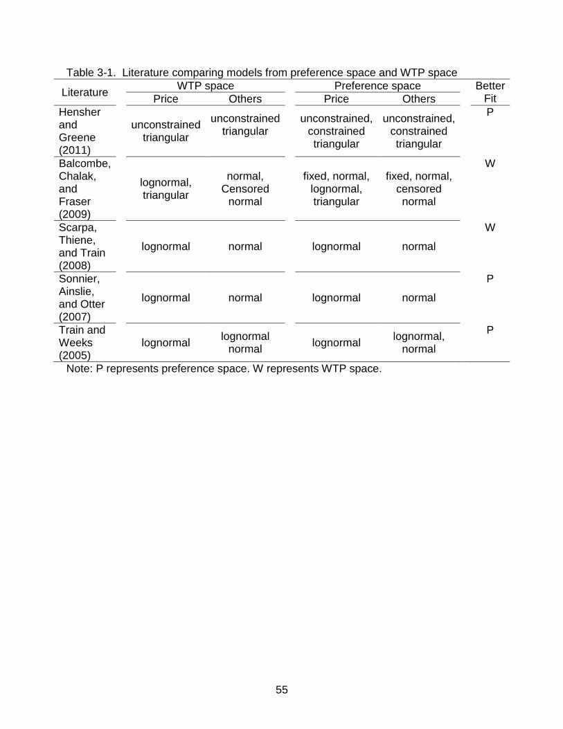
55
Table 3-1. Literature comparing models from preference space and WTP space
Literature WTP space Preference space Better
Fit Price Others Price Others
Hensher and Greene (2011)
unconstrained
triangular
unconstrained triangular
unconstrained, constrained triangular
unconstrained, constrained triangular
P
Balcombe, Chalak, and Fraser (2009)
lognormal, triangular
normal, Censored
normal
fixed, normal, lognormal, triangular
fixed, normal, censored normal
W
Scarpa, Thiene, and Train (2008)
lognormal normal lognormal normal
W
Sonnier, Ainslie, and Otter (2007)
lognormal normal lognormal normal
P
Train and Weeks (2005)
lognormal
lognormal normal
lognormal lognormal,
normal
P
Note: P represents preference space. W represents WTP space.
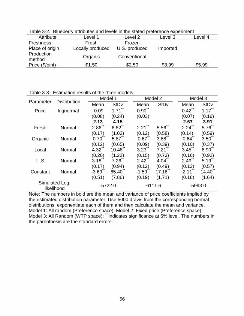
56
Table 3-2. Blueberry attributes and levels in the stated preference experiment
Attribute Level 1 Level 2 Level 3 Level 4
Freshness Fresh Frozen Place of origin Locally produced U.S. produced Imported Production method
Organic Conventional
Price ($/pint) $1.50 $2.50 $3.99 $5.99
Table 3-3. Estimation results of the three models
Parameter Distribution Model 1 Model 2 Model 3
Mean StDv Mean StDv Mean StDv
Price lognormal -0.09 (0.08)
1.71** (0.24)
0.90** (0.03)
0.42** (0.07)
1.17** (0.16)
2.13 4.15 2.67 3.91
Fresh Normal 2.86** (0.17)
8.82** (1.02)
2.21** (0.12)
5.56** (0.58)
2.24** (0.14)
5.76** (0.59)
Organic Normal -0.70** (0.12)
5.87** (0.65)
-0.67** (0.09)
3.88** (0.39)
-0.64** (0.10)
3.50** (0.37)
Local Normal 4.32** (0.20)
10.48**
(1.22) 3.23**
(0.15) 7.21** (0.73)
3.45** (0.16)
8.90** (0.92)
U.S Normal 3.18** (0.17)
7.26** (0.94)
2.42** (0.12)
4.04** (0.49)
2.49** (0.13)
5.19** (0.57)
Constant Normal -3.69** (0.51)
65.40**
(7.86) -1.59**
(0.19) 17.16**
(1.71) -2.11**
(0.18) 14.40** (1.64)
Simulated Log-likelihood
-5722.0 -6111.6 -5993.0
Note: The numbers in bold are the mean and variance of price coefficients implied by the estimated distribution parameter. Use 5000 draws from the corresponding normal distributions, exponentiate each of them and then calculate the mean and variance. Model 1: All random (Preference space); Model 2: Fixed price (Preference space); Model 3: All Random (WTP space); ** indicates significance at 5% level. The numbers in the parenthesis are the standard errors.
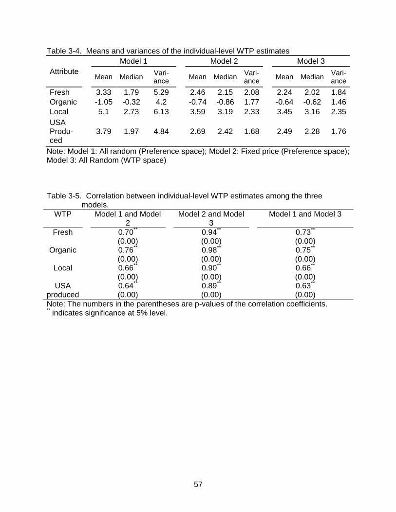
57
Table 3-4. Means and variances of the individual-level WTP estimates
Attribute
Model 1 Model 2 Model 3
Mean Median
Vari-ance
Mean Median Vari-ance
Mean Median Vari-ance
Fresh
3.33 1.79 5.29
2.46 2.15 2.08
2.24 2.02 1.84
Organic
-1.05 -0.32 4.2
-0.74 -0.86 1.77
-0.64 -0.62 1.46
Local
5.1 2.73 6.13
3.59 3.19 2.33
3.45 3.16 2.35
USA Produ-ced
3.79 1.97 4.84 2.69 2.42 1.68 2.49 2.28 1.76
Note: Model 1: All random (Preference space); Model 2: Fixed price (Preference space); Model 3: All Random (WTP space) Table 3-5. Correlation between individual-level WTP estimates among the three
models.
WTP Model 1 and Model 2
Model 2 and Model 3
Model 1 and Model 3
Fresh 0.70** (0.00)
0.94** (0.00)
0.73** (0.00)
Organic 0.76** (0.00)
0.98**
(0.00) 0.75**
(0.00) Local 0.66**
(0.00) 0.90**
(0.00) 0.66**
(0.00) USA
produced
0.64** (0.00)
0.89** (0.00)
0.63** (0.00)
Note: The numbers in the parentheses are p-values of the correlation coefficients. ** indicates significance at 5% level.
58
CHAPTER 4 CONSUMERS’ WILLINGNESS-TO-PAY FOR ORGANIC AND LOCAL BLUEBERRIES:
A MULTI-STORE BDM AUCTION CONTROLLING FOR PURCHASE INTENTIONS
4.1 Introduction
The Becker-DeGroot-Marschak method (BDM) is well suited for field experimental
auctions (Becker, Degroot, and Marschak, 1964), and as a result, has been increasingly
used by researchers in the area of consumer behavior to elicit consumers’ valuation of
food (Wertenbroch and Skiera, 2002; Carrigan and Rousu, 2008; Silva et al., 2007;
Rozan et al., 2004; Rousu et al., 2005 and Lusk et al., 2001 etc.). The most common
location for conducting a BDM auction focusing on consumers’ valuation of food is
grocery stores and the procedure is relatively simple compared with other auction
formats. In a typical BDM auction, the participant places a bid for the auctioned product
and then draws a random price. If the randomly drawn price is greater than the bid, the
participant does not “win” the product and pays nothing. If the randomly drawn price is
below the bid, the participant “wins” the product and pays the price he/she draws.
The bidding behavior of participants is affected by many factors. Consumers’
cognitive structure is complex and a lot of questions still remain unanswered. Many
researchers have accepted the theory that instead of having fixed or previously formed
values, consumers often construct different assessment contingent on different spots
or choice contexts (Tversky and Simonson 1993; Payne, Bettman, and Johnson
1992; Bettman, Luce, and Payne 1998). Horowitz (2006) argued that people’s
valuation of an item is correlated with the circumstances in which he/she is going to pay
for it.
People go to grocery stores to buy food, so whether they intend to buy the
auctioned products when the auction is conducted might be a factor that would affect
59
the participants’ bids. Since real money is usually involved in the auction process, if
auction participants do not plan to purchase the auctioned products, they may bid less
than they usually pay for the product and use the money for the products that they plan
to purchase. Corrigan and Rousu (2008) argued that purchase intention critically
determined consumers’ willingness-to-pay (WTP) for perishable goods. They found that
auction participants who planned to buy the auctioned products that day submitted bids
equal to their perceived market prices of the products while participants who did not
have such plan submitted bids less than the market prices. People report valuation
according to their goals at that time, task environment, description of the task and
product information etc. (Bettman et al. 1998). In this regard, it’s necessary to control
more factors, though many of which might be difficult to measure, that can influence
consumers’ bidding behavior.
Another important point worth attention for BDM auctions is the choice of auction
locations. One of the biggest advantages of BDM auctions over the other auction
formats is its point-of-purchase locations, which offer participants a more realistic choice
situation (Carson et al. 1994). However, the locations should be chosen with caution
and the potential impact of location choices on auction results should be considered.
There are many types of marketing outlets that feature different types of food (e.g.
organic, local etc.). Food quality, availability and price expectations may differ
depending on the location of purchase. The co-existence of different marketing outlets
indicates that consumers have different demands and expectations for food. These
different attitudes toward food may drive a consumer to select an outlet they believe to
satisfy their demand for specific attributes. For example, people who prefer organic food
60
may go to a high-end grocery store that features organic food, or to outlets like farmers’
markets. People who prefer locally produced food may shop at a farmers’ market.
Differences in prices, food quality or availability of organic or local fruit across different
locations may cause differences in people’s valuation of food products sold at these
locations. Since there are numerous types of marketing outlets that attract different
consumer groups, the generalizability of a BDM auction result conducted at only one
store, or one store type, is questionable. For example, if one were to investigate the
WTP for a local food product, but conducted BDM auctions at a grocery store, they
might be missing a segment of the population that values local higher and purchases
their good from farmers markets. On the other hand, if the auction is only conducted at
the farmer’s market, the valuation might represent a subset that values the attribute
more than the average consumer. Thus, if a broader, more complete picture of
consumer demand for attributes is wanted, reaching more consumer types than found
at one type of location may be needed.
In this study, we extend previous literature in two directions. First, we extend the
study by Corrigan and Rousu to explore the effect of purchase intentions on partial bids
(e.g. for a value-added attribute of the products) in addition to full bids (for the whole
products). Researchers are often interested in consumers’ WTPs for product attributes
instead of the whole product. As such, it is important to understand the impact of
purchase intention on consumers’ partial bids for product attributes in experimental
auctions to provide a recommendation for the need to control for this variable in studies
that focus on attributes over whole products.
61
Second, we conduct BDM auctions in three different types of marketing outlets:
grocery stores that focus on delivering products at the lowest price (price-conscious),
grocery stores that focus on high quality (quality-focused), and farmers’ markets.
Although previous literature did explore the impact of conducting auctions at the point of
purchase, such as grocery stores (Lust and Fox 2003; Shogren et al. 1999 etc.), the
experiment was usually conducted only in one type of location. Although there are
studies that determined the difference in consumers’ attitudes toward food product
attributes in different countries (Lusk et al. 2004; Lusk, Roosen, and Fox 2003), little
research has been conducted using auctions to consider whether such differences also
exist across different types of marketing outlets. If such difference does exist, it may be
recommended that field auctions be conducted in multiple locations or locations with
consumers who are more representative of the population being studied so that the
auction results can be generalized.
The study seeks to answer the following questions:
1. How does participants’ purchase intention affect their bidding behavior for
partial bids and full bids?
2. Will the BDM auction yield different results at different marketing outlets?
4.2 Literature Review
Literature has revealed exaggerated willingness-to-pay (WTP) estimates due to
the hypothetical nature of some valuation methods. For example, List and Gallet (2001)
suggested that on average, preference in the hypothetical setting was inflated by a
factor of 3. Therefore, researchers began to rely on non-hypothetical methods, such
as experimental auctions (EA), to elicit consumers’ WTP for products or additional
62
attributes (Rozan et al. 2004; Jaeger et al. 2004; Melton et al. 1996; Huffman et al.
2003, Hayes et al. 2002, Bernard and Bernard 2009, Hayes et al. 1995, Umberger
et al. 2002, Alfnes and Rickertsen 2003 etc.).
Over time, locations of experimental auctions were no longer limited to labs and
have been extended to more realistic contexts, such as grocery stores, or other point of
purchase locations (Rozan et al. 2004; Rousu et al. 2005; Lusk and Fox, 2003; Lusk et
al. 2001; Silva et al. (2007); List 2001 and List and Lucking-Reiley 2000 etc.). While lab
auctions have been used widely to elicit people’s attitudes toward non-market goods
(i.e., environment conservation, food safety and novel good), field auctions have been
gaining popularity in the valuation of market goods and empirical consumer behavior
studies. Auctions conducted in a retail context have a number of advantages over lab
auctions, such as a more realistic circumstance for participants, a better capture of the
target population and reduced compensation and recruiting fees for the investigator
(Lust and Fox 2003; Lusk et al. 2001). Carson et al. (1994) argued that the choice
context of value elicitation should be as close as possible to the real purchase situation.
Wertenbroch and Skiera (2002) found that different from hypothetical methods, there
was no overbidding in BDM auctions. Carrigan and Rousu (2008) concluded that
participants in the BDM auction understood that the auction was demand revealing,
which indicated that their bids were unbiased.
However, literature has reported value elicitation results that are inconsistent with
basic preference theories. For example, in a sports card auction conducted in a sports
card show, List (2002) found that the superior bundle was preferred when juxtaposed
with the inferior bundle. However, when in isolation, the inferior bundle was valued
63
much higher. The paper argued that the dichotomous choice questions might be
challenged and various other nonmarket valuation methods should be examined. Thaler
(1985) showed that people’s stated WTP for the same product (cold beer) differed
dramatically across different points of purchase (a run-down grocery store and a fancy
hotel). Additionally, despite many studies that concluded with exaggerated WTP
estimates in hypothetical context (Lusk and Schroeder 2004; List and Shogren 1998;
Shogren et al. 1999 etc.), Lusk and Fox (2003) found that auctions conducted in stores
yielded larger bids than lab auctions, given that participants were happy to participate
and were not constrained by cash (not having enough cash to pay for the auctioned
product if they win).
More research is needed to understand the inconsistencies that have been found.
Irwin et al. (1993) argued that people actually do not have an exact monetary value for
goods, except for those very simple and familiar. As a way to explain the gap between
theory and action, numerous studies have been done to test the generalizability of
previous findings by controlling more consumer-side, environment-side, or
methodology-side factors that might deviate from theoretical assumptions and affect
consumer behavior in research experiments. For example, on the consumer-side, Lusk
and Fox (2003) analyzed auction results controlling for “unengaged bidders (participants
that bid zero for all the products)”. Corrigan and Rousu (2008) analyzed the effect of
purchase intentions on consumers’ bidding behavior. List (2001) studied the use of
“cheap talk” (an explicit warning or explanation why it is important to bid the true WTP
value) on reducing hypothetical bias in elicitation procedures. The results were shown to
depend on participants’ experience with the auctioned good. Additionally, List and Gallet
64
(2001) argued that the extent of over-statement of preferences was related to the
distinction between public and private goods, WTP and willingness-to-accept (WTA)
and different elicitation methods. Such empirical findings serve as useful warnings for
researchers that unobserved factors might impact consumers’ reported valuation of
products, and should be controlled for when possible in experimental auctions.
4.3 Auction Procedure
A series of BDM auctions were conducted in July and August 2011 in Pittsburgh,
Pennsylvania and Orlando, Florida. In each city, two grocery stores (one price-
conscious and one quality-focused) and a farmers’ market were selected.
Approximately 70 observations were collected in each location, with a total number of
qualified observations of 356. The auctions were set up at the entrance to the stores
and near the beginning of the farmers’ markets. Consumers to the outlets were
randomly stopped and asked whether they would like to participate in an experiment
about food consumption. Qualified consumers (adult, blueberry consumers without food
allergies) were asked to fill out a questionnaire about purchase intention, demographics
etc.
Four types of blueberries (organic and locally produced blueberries, conventional
and locally produced blueberries, organic blueberries produced in the U.S. and
conventional blueberries produced in the U.S.) were auctioned. Before the auction,
each participant was given a sheet explaining the auction procedure. The auctioneer
then explained the auction procedure to the participants and answered questions from
the participants about the procedure.
The auction procedure had four steps:
65
1. Each participant was endowed with $7 cash, which they were told could be
used to purchase the blueberries if they won the auction or was theirs to keep if they did
not win. The participants were asked to bid simultaneously for four types of blueberries
in one-pint clamshell packages. The auctioneer explained to the participant that it was
his/her best interest to bid exactly what he/she was willing to pay for each blueberry
package.
2. After the participants placed the bids, they randomly drew a letter to determine
which blueberry was actually auctioned. Therefore, they only had the opportunity to buy
one type of blueberries.
3. Once the auctioned blueberry type was determined, participants were asked to
draw a random price.
4. If a participant’s bid for the randomly selected blueberries was higher than the
price drawn for those blueberries, the participant purchased the blueberries at the
randomly drawn price. If a participant’s bid for the blueberries was lower than the drawn
price, the participant did not purchase the blueberries.
4.4 Results
A demographic summary of participants at each marketing outlet is shown in Table
4-1. Demographics does differ by location, with the price-conscious marketing outlet
featuring consumers who tended to be younger, had lower income, had a lower
education level, and were more likely to be Black or African American. They also tended
to have more children than consumers at the other two marketing outlets. The
participants at the farmers’ markets have the highest average income and education
level. The variation in demographics at different marketing outlets indicates that the
auctions may produce different full bids and partial bids at different locations.
66
Summary statistics for the four bids for the four types of blueberries at each
marketing outlet are shown in Table 4-2. The bids for organic, local blueberries (bid1);
conventional, local blueberries (bid2); and conventional, U.S. produced blueberries
(bid4) are the highest in the farmers’ markets and the lowest in the price-conscious
stores. The bids for organic, U.S. produced blueberries (bid3) are the highest in the
quality-focused stores and the lowest in the price-conscious stores.
4.4.1 Partial Bids for Organic and Local Blueberries at Different Marketing Outlets
In the survey before the auction, information on attitudes toward organic and local
fruits was collected. Significant differences are found among the answers from
participants at different locations. Specifically, participants at the quality-focused grocery
stores demonstrate more trust in organic fruits than participants at the price-conscious
grocery stores. They are more likely to agree to a statement that they will pay more for
fruits with an organic label than participants at the price-conscious grocery stores (on a
5-point Likert scale). Participants from the two farmers’ markets are generally more
likely to indicate that they will purchase local blueberries than those from the other two
locations (on a 5-point Likert scale).
The means and standard deviations of bids for organic and local blueberries at
different marketing outlets are shown in Table 4-3. According to the Bonferroni multiple
comparison test, participants at the quality-focused stores, which are known for selling
organic food, have higher bids for organic blueberries than participants at the price-
conscious grocery stores. For local blueberries, the farmers’ markets have the highest
bids among the three marketing outlets. The results are consistent with our expectation
that the experiment will yield higher bids for organic blueberries in quality-focused
67
grocery stores and higher bids for local blueberries in farmers’ market. Additionally, the
bids for organic blueberries are larger than the bids for local blueberries, no matter
where the auction was conducted. This indicates that consumers generally consider the
organic production of blueberries a more important attribute than production location.
However, the standard deviations of bids for organic blueberries are all bigger than
those for local blueberries. Therefore, more divergence exists in consumers’ attitudes
toward the organic production of blueberries.
4.4.2 Impact of Purchase Intention
Since fresh blueberry is a highly perishable fruit, it’s reasonable to expect that
people will bid differently if they plan to buy blueberries on the day of auction. To control
for such impact, participants were asked to indicate if they planned on purchasing fresh
blueberries at the store/market. Participants from different marketing outlets but with the
same purchase intentions are grouped together to test if purchase intentions impact
bids. The Bonferroni multiple comparison test is used to detect pairwise differences for
full bids as well as partial bids between different groups. The results are summarized in
Table 4-4.
Significant differences exist between the full bids of participants with purchase
intentions and the full bids of participants without purchase intension for all the four
types of blueberries. The differences in the full bids between participants without
purchase intention and those who are not sure if they planned to purchase are not all
significant (Only the differences for bid3 and bid4 are significant). This result is
consistent with previous findings that consumers who plan to buy the auctioned
products tend to have higher bids than those who do not intend to buy the auctioned
products. However, the partial bids for local or organic blueberries are not significantly
68
different across groups with different purchase intentions. Therefore, although purchase
intention has effects on the full bids in the auction, it does not affect the revelation of the
relative values among multiple auctioned products. This indicates that the impacts of
purchase intention on products are in same direction and with similar scale such that
the partial bids calculated as the difference between the full bids for various products do
not vary among consumers with different purchase intentions.
4.4.3 The Tobit Model for Full Bids
To investigate the relationship between reported full bids and participants’
demographics, attitudes, auction location and auctioned blueberry type, a Tobit model is
used since the dependent variable (reported bids) is left censored at zero. The model is
specified as follows:
If * 0iBid ,
*
0 1 2 3 4 5
6 6 _ 0
i i i i i i
i
Bid Bid X FM Qualityfocused Florida Organic
Local Organic local
(4-1)
If * 0, 0i iBid Bid
*
iBid is the latent dependent variable and iBid is the observed dependent variable.
iX is the vector of demographic and attitude independent variables that include age,
gender, income, race, education level, number of children in the household, how well
participants like fresh blueberries, whether they had purchased fresh blueberries before
and whether they intended to buy fresh blueberries that day. iFM and iQualityfocused are
the dummy variables for the farmers’ markets and the quality-focused stores
respectively. Florida is the dummy variable for Florida auction participants. Organic ,
Local and _Organic local indicate the blueberry types. The dummy variables for price-
69
conscious stores and Pennsylvania are omitted for identification purpose. i is the error
term. The regression results are shown in Table 4-5.
For the demographic independent variables, age, Asian and college education are
significant. Age and Asian are significantly negative, indicating that older participants bid
less than younger participants and Asian participants bid less than African-American
participants (African-American is omitted for identification purpose). Participants with
college degrees bid significantly higher than those without a college degree.
Surprisingly, no significant difference is found between the bids of postgraduates and
participants without college education.
The coefficients of the variables indicating blueberry types are all significantly
positive. Therefore, both value-added attributes (organic and local) of blueberries attract
some price premiums from the auction participants. The result also shows that
consumers are willing to pay more for organic blueberries than for locally produced
blueberries.
Dummy variables for the marketing outlets are significant with the bids at the
farmers’ markets and the quality-focused stores significantly higher than those at the
price-conscious stores. This result is as expected since these two stores are intended to
attract more consumers who seek high-quality food and thus are relatively less price-
conscious. Importantly, this holds after controlling for the demographic differences
among marketing outlets and blueberry types, implying that participants’ full bids do
differ among different types of stores. In addition to marketing outlets, the location of the
auctions was significant. Participants from Florida bid significantly lower than those from
Pennsylvania.
70
As expected, how well the participants like fresh blueberries has a significant
positive effect on the reported full bids. However, the purchase history (whether the
participant had purchased fresh blueberries before) is not significant, which indicates
that familiarity with blueberries does not affect participants’ full bids. For purchase
intention, participants planning to buy fresh blueberries on the day of auction bid
significantly higher than those who did not have such plans. This is also consistent with
the results in Table 4-2.
4.4.4 The OLS Regression for Partial Bids
To investigate how the independent variables in Equation (1) affect the partial
bids, the same set of independent variables, with the exception of the dummy variables
for blueberry types are regressed on partial bids for organic and local blueberries.
The partial bids for organic are calculated as the difference between bids for organic,
U.S. produced blueberries and conventional, U.S. produced blueberries and the partial
bids for local are calculated as the difference between bids for conventional, local
blueberries and conventional, U.S. produced blueberries. In both cases, there are both
positive and negative signs, thus, we use a robust OLS regression. The models are
specified as follow:
0 1 2 3 4iorg i i i i iWTP X FM Qualityfocused Florida (4-2)
0 1 2 3 4ilocal i i i i iWTP X FM Qualityfocused Florida (4-3)
iorgWTP and ilocalWTP are observed dependent variables. The regression results are
illustrated in Table 4-6. Many variables that were significant in the model for full bids
become insignificant in the model for partial bids. In the model for local blueberries, only
age and the two store dummy variables are significant. As expected, the coefficients for
71
the two store dummy variables are significantly positive, which is a reasonable result
since participants from these two types of marketing outlets are more quality-focused or
more likely to care about place of origin of food. This result also holds when
demographic differences among the stores are controlled for. For organic blueberries,
only age, female and the dummy for quality-focused store are significant. Female
consumers are more willing to pay premiums for organic blueberries than males, which
suggests that females are more interested in organic food products than males. The
significance of the coefficient for the quality-focused stores indicates that consumers in
this type of store place more emphasis on the organic production of blueberries than
consumers from the other two types of stores.
Purchase intentions are insignificant in both models. This also confirms our
previous results that purchase intentions have no effect on partial bids. Additionally,
purchase history does not affect participants’ partial bids for the value-added attribute of
“organic” or “local”.
4.5 Conclusion
In this study, a series of BDM auctions were conducted to elicit consumers’
valuation of organic and locally produced blueberries. We argue that the purchase
intention of auction participants and the choice of auction location could impact
participants’ bidding behavior. We extend the study of Corrigan and Rousu (2008) by
analyzing the effect of purchase intentions on partial bids as well as full bids. In addition,
the auctions were conducted at three types of marketing outlets: price-conscious
grocery stores, farmers’ markets and quality-focused grocery stores to capture a more
diverse sample of consumers.
72
Our results show that purchase intention on the day of the auction only affects full
bids, but not partial bids (e.g. bids for a value-added attribute). Auction participants who
planned to purchase the auctioned product reported higher bids than those who did not
plan to purchase. However, the partial bids were consistent among participants with
different purchase intentions. Therefore, future research on partial bids might be less
dependent on participants’ purchase intentions. However, future research is needed to
determine if these results hold only for perishable goods, or for all types of products.
It was also found that there are differences in demographics among consumers,
as well as their attitudes toward organic and local production of fruits at different
marketing outlets. Even after controlling for the demographics and attitudes difference,
bids for “organic” and “local” were significantly different at different marketing outlets.
Specifically, consumers in the farmers’ markets had the highest partial bids for local
blueberries while consumers in the quality-focused stores had the highest partial bids
for organic blueberries. Therefore, if the auction was conducted at only one type of
marketing outlet, the bids might be underestimated or overestimated, even if
demographics and intentions are controlled for. Our study also indicates that
consumers’ attitudes toward organic production of blueberries demonstrate more
variation than their attitudes toward locally produced blueberries.
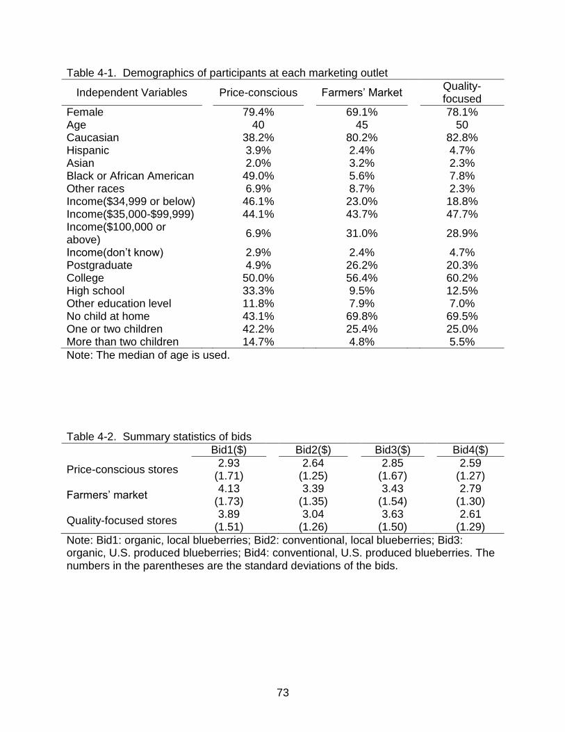
73
Table 4-1. Demographics of participants at each marketing outlet
Independent Variables
Price-conscious
Farmers’ Market Quality-
focused
Female 79.4% 69.1% 78.1% Age 40 45 50 Caucasian 38.2% 80.2% 82.8% Hispanic 3.9% 2.4% 4.7% Asian 2.0% 3.2% 2.3% Black or African American 49.0% 5.6% 7.8% Other races 6.9% 8.7% 2.3% Income($34,999 or below) 46.1% 23.0% 18.8% Income($35,000-$99,999) 44.1% 43.7% 47.7% Income($100,000 or above)
6.9%
31.0%
28.9%
Income(don’t know) 2.9% 2.4% 4.7% Postgraduate 4.9% 26.2% 20.3% College 50.0% 56.4% 60.2% High school 33.3% 9.5% 12.5% Other education level 11.8% 7.9% 7.0% No child at home 43.1% 69.8% 69.5% One or two children 42.2% 25.4% 25.0% More than two children 14.7% 4.8% 5.5%
Note: The median of age is used.
Table 4-2. Summary statistics of bids
Bid1($) Bid2($) Bid3($) Bid4($)
Price-conscious stores 2.93
(1.71)
2.64 (1.25)
2.85
(1.67)
2.59 (1.27)
Farmers’ market 4.13
(1.73)
3.39 (1.35)
3.43
(1.54)
2.79 (1.30)
Quality-focused stores 3.89
(1.51)
3.04 (1.26)
3.63
(1.50)
2.61 (1.29)
Note: Bid1: organic, local blueberries; Bid2: conventional, local blueberries; Bid3: organic, U.S. produced blueberries; Bid4: conventional, U.S. produced blueberries. The numbers in the parentheses are the standard deviations of the bids.
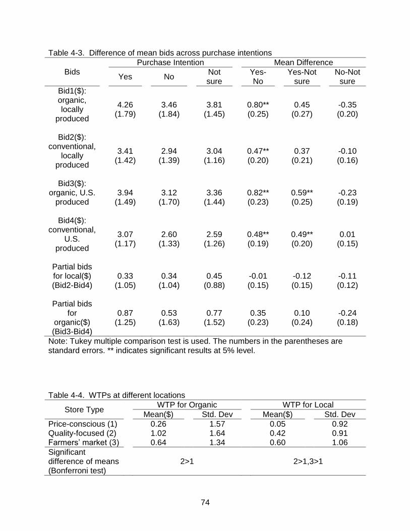
74
Table 4-3. Difference of mean bids across purchase intentions
Bids Purchase Intention Mean Difference
Yes
No
Not sure
Yes-No
Yes-Not sure
No-Not sure
Bid1($): organic, locally
produced
4.26 (1.79)
3.46 (1.84)
3.81 (1.45)
0.80** (0.25)
0.45 (0.27)
-0.35 (0.20)
Bid2($): conventional,
locally produced
3.41 (1.42)
2.94 (1.39)
3.04 (1.16)
0.47** (0.20)
0.37 (0.21)
-0.10 (0.16)
Bid3($): organic, U.S.
produced
3.94
(1.49)
3.12
(1.70)
3.36
(1.44)
0.82** (0.23)
0.59** (0.25)
-0.23 (0.19)
Bid4($): conventional,
U.S. produced
3.07 (1.17)
2.60 (1.33)
2.59 (1.26)
0.48** (0.19)
0.49** (0.20)
0.01 (0.15)
Partial bids for local($) (Bid2-Bid4)
0.33
(1.05)
0.34
(1.04)
0.45
(0.88)
-0.01 (0.15)
-0.12 (0.15)
-0.11 (0.12)
Partial bids for
organic($) (Bid3-Bid4)
0.87
(1.25)
0.53
(1.63)
0.77
(1.52)
0.35
(0.23)
0.10
(0.24)
-0.24 (0.18)
Note: Tukey multiple comparison test is used. The numbers in the parentheses are standard errors. ** indicates significant results at 5% level.
Table 4-4. WTPs at different locations
Store Type WTP for Organic WTP for Local
Mean($) Std. Dev Mean($) Std. Dev
Price-conscious (1) 0.26 1.57 0.05 0.92 Quality-focused (2) 1.02 1.64 0.42 0.91 Farmers’ market (3) 0.64 1.34 0.60 1.06
Significant difference of means (Bonferroni test)
2>1 2>1,3>1
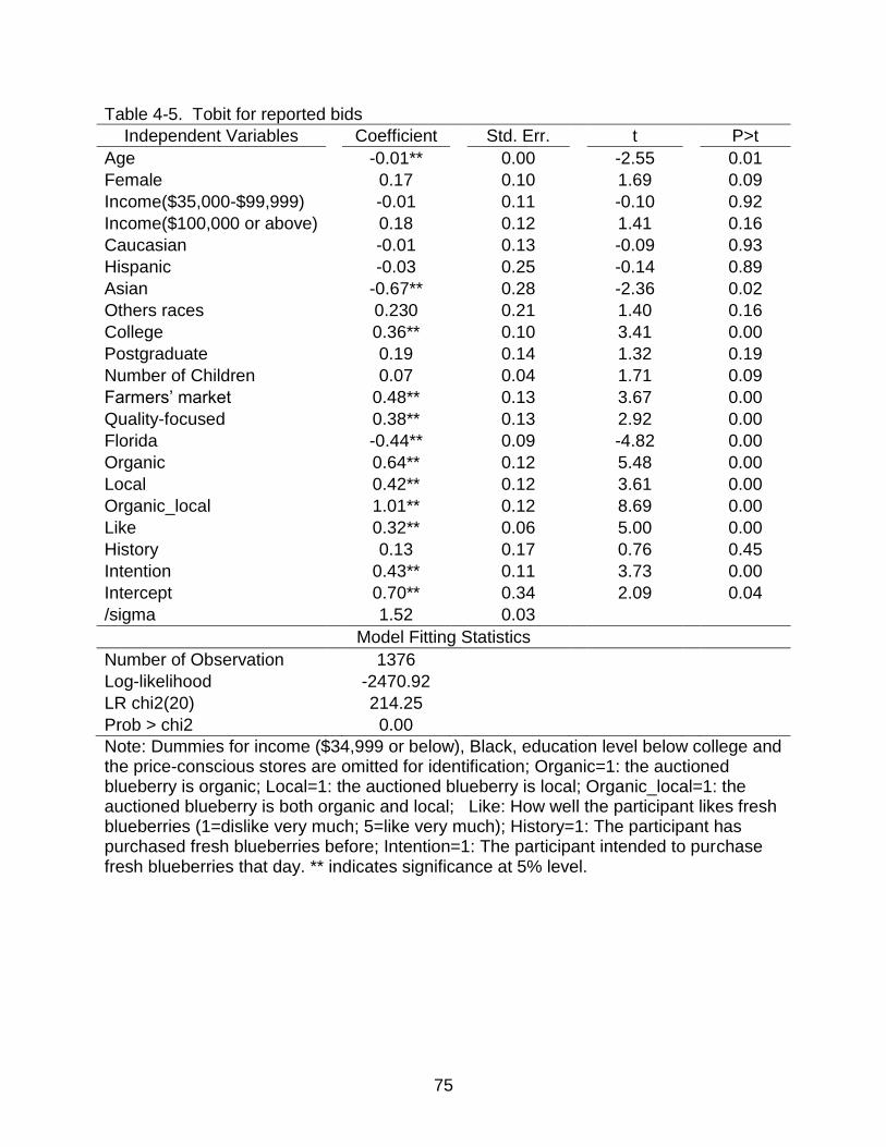
75
Table 4-5. Tobit for reported bids
Independent Variables Coefficient Std. Err. t P>t
Age -0.01** 0.00 -2.55 0.01
Female 0.17 0.10 1.69 0.09
Income($35,000-$99,999) -0.01 0.11 -0.10 0.92
Income($100,000 or above) 0.18 0.12 1.41 0.16
Caucasian -0.01 0.13 -0.09 0.93
Hispanic -0.03 0.25 -0.14 0.89
Asian -0.67** 0.28 -2.36 0.02
Others races 0.230 0.21 1.40 0.16
College 0.36** 0.10 3.41 0.00
Postgraduate 0.19 0.14 1.32 0.19
Number of Children 0.07 0.04 1.71 0.09
Farmers’ market 0.48** 0.13 3.67 0.00
Quality-focused 0.38** 0.13 2.92 0.00
Florida -0.44** 0.09 -4.82 0.00
Organic 0.64** 0.12 5.48 0.00
Local 0.42** 0.12 3.61 0.00
Organic_local 1.01** 0.12 8.69 0.00
Like 0.32** 0.06 5.00 0.00
History 0.13 0.17 0.76 0.45
Intention 0.43** 0.11 3.73 0.00
Intercept 0.70** 0.34 2.09 0.04
/sigma 1.52 0.03
Model Fitting Statistics
Number of Observation 1376
Log-likelihood -2470.92
LR chi2(20) 214.25
Prob > chi2 0.00
Note: Dummies for income ($34,999 or below), Black, education level below college and the price-conscious stores are omitted for identification; Organic=1: the auctioned blueberry is organic; Local=1: the auctioned blueberry is local; Organic_local=1: the auctioned blueberry is both organic and local; Like: How well the participant likes fresh blueberries (1=dislike very much; 5=like very much); History=1: The participant has purchased fresh blueberries before; Intention=1: The participant intended to purchase fresh blueberries that day. ** indicates significance at 5% level.
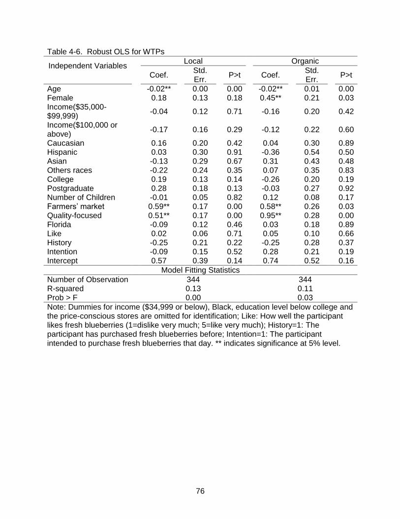
76
Table 4-6. Robust OLS for WTPs
Independent Variables Local Organic
Coef. Std. Err.
P>t Coef. Std. Err.
P>t
Age -0.02** 0.00 0.00 -0.02** 0.01 0.00 Female 0.18 0.13 0.18 0.45** 0.21 0.03 Income($35,000-$99,999)
-0.04 0.12 0.71 -0.16 0.20 0.42
Income($100,000 or above)
-0.17 0.16 0.29 -0.12 0.22 0.60
Caucasian 0.16 0.20 0.42 0.04 0.30 0.89 Hispanic 0.03 0.30 0.91 -0.36 0.54 0.50 Asian -0.13 0.29 0.67 0.31 0.43 0.48 Others races -0.22 0.24 0.35 0.07 0.35 0.83 College 0.19 0.13 0.14 -0.26 0.20 0.19 Postgraduate 0.28 0.18 0.13 -0.03 0.27 0.92 Number of Children -0.01 0.05 0.82 0.12 0.08 0.17 Farmers’ market 0.59** 0.17 0.00 0.58** 0.26 0.03 Quality-focused 0.51** 0.17 0.00 0.95** 0.28 0.00 Florida -0.09 0.12 0.46 0.03 0.18 0.89 Like 0.02 0.06 0.71 0.05 0.10 0.66 History -0.25 0.21 0.22 -0.25 0.28 0.37 Intention -0.09 0.15 0.52 0.28 0.21 0.19 Intercept 0.57 0.39 0.14 0.74 0.52 0.16
Model Fitting Statistics
Number of Observation 344 0.13 0.00
344 0.11 0.03
R-squared Prob > F
Note: Dummies for income ($34,999 or below), Black, education level below college and the price-conscious stores are omitted for identification; Like: How well the participant likes fresh blueberries (1=dislike very much; 5=like very much); History=1: The participant has purchased fresh blueberries before; Intention=1: The participant intended to purchase fresh blueberries that day. ** indicates significance at 5% level.
77
CHAPTER 5 CONCLUSION
Understanding consumers’ preferences and attitudes is critical for new product
development, labeling policy formulation or the prediction of product market shares.
However, the measurement of preferences and attitudes could be difficult as they are
both abstract concepts. Willingness-to-pay (WTP), as a measurable concept, has
enabled people to have a one-to-one correspondence between preference and
monetary values.
Studies that used different methodologies could yield different WTP values.
Therefore, researchers have been exploring ways to get an unbiased WTP values.
Some commonly used value elicitation methods include contingent valuation,
experimental auctions etc. Although these methods have been used and discussed for
a long time, research is still ongoing about methods that will give us more accurate
measurement.
In this dissertation, attempts have been made to discover some problems and
methodological improvement in the process of eliciting WTPs. Two value elicitation
methods: choice experiment and experimental auction are discussed. The research
subject is consumers’ WTP for blueberry attributes. As a fruit containing high level of
nutrients, the blueberry has an expanding consumer group but studies about
consumers’ attitude toward blueberry attributes are quite limited.
For the indirect methods to calculate WTPs, such as the choice experiment, the
models used to estimate WTPs are among the hottest discussed topics. Researchers
have found a lot of inconsistencies between various value elicitation methods. However,
different models can also result in different results with the same data. In Chapter 2 of
78
this dissertation, a hypothetical method: a choice experiment, is used to compare
consumers’ attitudes toward three blueberry attributes: freshness, organic or not, and
place of production (local, U.S. produced or imported). The all random WTP space
mixed logit model is used for parameter estimation. The results indicate that consumers
in the U.S. regard the local production of blueberries a more important attribute than
whether they are organic or not. Even though there is a fair amount of consumers that
are willing to pay positive premiums for organic blueberries, the majority of them don’t
have positive WTPs for the “organic” attribute. Additionally, we conclude that
disaggregate information, which can be derived from the Bayesian estimation method,
is more useful for target marketing.
In Chapter 3, three widely used specifications for mixed logit are estimated and
compared. The results show that the divergence found in previous literature between
the preference space model and the WTP space model can be narrowed when the price
coefficient is assumed fixed in the preference space. The results suggest that the fixed
price preference space model might be used as a substitute for the all random WTP
space model, which is used in Chapter 2. This is an interesting finding as the all random
WTP space model need extra steps in estimation and may also suffer from the
identification problems suggested by Ruud (1996). This chapter reaches the same
conclusion as Chapter 2 in terms of the attribute importance rankings of blueberries.
Although the choice experiment is relatively easy for researchers to implement and
straightforward for consumers to understand, hypothetical bias has been one of its most
questioned problems. For direct methods, such as experimental auctions, the problem
of hypothetical bias has been dealt with, but the choices of the auction format, auction

79
locations and specific auction procedures are other problems that need serious
consideration for the experiment to be incentive-compatible.
In Chapter 4, a non-hypothetical method: experimental auction is conducted for
consumers’ WTP for organic and local blueberries. The WTP estimates from the
experimental auction are much smaller than those from the choice experiment.
Therefore, our results are consistent with previous studies in that the choice experiment
tends to provide exaggerated WTP estimates. Additionally, we find that auction
participants’ purchase intentions on the day of auction and the choice of auction
locations have significant impact on participants’ bidding behavior. Specifically,
purchase intentions affect full bids, but not partial bids while the choice of auction
locations affects both full bids and partial bids. Even though the experiment auctions
might provide more plausible WTP estimates than choice experiments, the reliability of
the results from experimental auctions has not been verified. A variety of observable or
unobservable factors might impact consumers’ bidding behavior in the auction process.
More research should be done to discover and evaluate these factors so that a better
reflection of consumers’ preferences can be revealed.
Apart from the findings regarding methodologies, Chapters 2 and 3 and Chapter 4
give contradictory results on the importance comparison between “organic” and “local”.
Although most literature also found different WTP values with different value elicitation
methods, little of them have found inconsistent attribute importance rankings. One of the
reasons might be that in the choice experiment, the organic attribute was ignored
because there were too many attributes to be compared in each choice situation. In the
auction process, however, there were only two attributes: “organic” and “local”. Another

80
reason might be that the comparison is based on WTP means, which are subject to the
influence of extreme values. This contradiction might also indicate that the design of
choice experiments needs extra caution or more studies should be conducted on the
reliability of the estimates from choice experiments.

81
APPENDIX A CHOICE SITUATIONS FOR THE CHOICE EXPERIMENT
Which of the following two choices for blueberries would you pick?
. . .
Q97
Which of the following two choices for blueberries would you pick?
. . .
Q98
Which of the following two choices for blueberries would you pick?
. . .
Q99
Which of the following two choices for blueberries would you pick?
. . .
Q100
Which of the following two choices for blueberries would you pick?

82
. . .
Q101
Which of the following two choices for blueberries would you pick?
. . .
Q102
Which of the following two choices for blueberries would you pick?
. . .
Q103
Which of the following two choices for blueberries would you pick?
. . .
Q104
Which of the following two choices for blueberries would you pick?
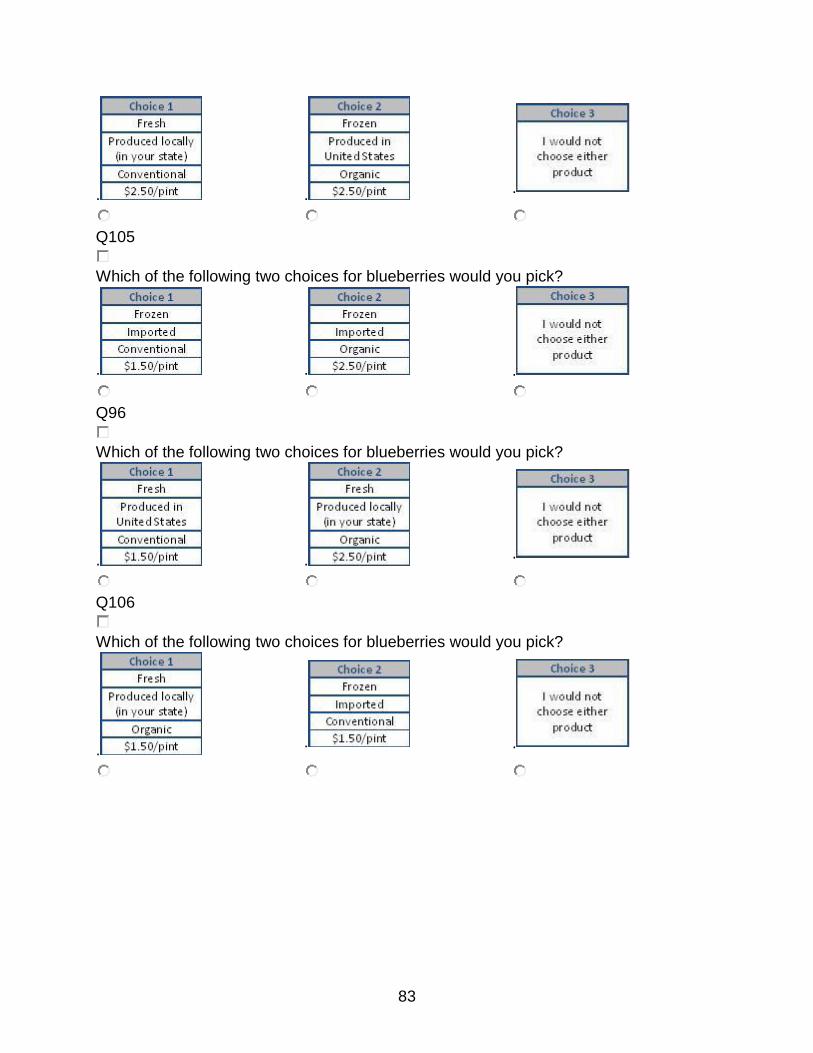
83
. . .
Q105
Which of the following two choices for blueberries would you pick?
. . .
Q96
Which of the following two choices for blueberries would you pick?
. . .
Q106
Which of the following two choices for blueberries would you pick?
. . .

84
APPENDIX B BDM AUCTION QUESTIONNAIRE
Have you ever purchased fresh blueberries?
⃝ Yes
⃝ No
Approximately how much money did you spend on fresh blueberries in the LAST
MONTH?
⃝ Nothing, I did not purchase fresh blueberries last month
⃝ Less than $4
⃝ $4.00 - $9.99
⃝ $10.00 - $14.99
⃝ $15.00 - $19.99
⃝ $20.00 - $29.99
⃝ $30 or more
Is this the location where you typically purchase most of your fruit from?
⃝ Yes
⃝ No
Did you intend to purchase fresh blueberries here today?
⃝ Yes
⃝ No
⃝ Not sure
Do you currently have any fresh blueberries at home?
⃝ Yes
⃝ No
What state do you currently live in (at least 6 months out of the year)?
⃝ Florida
⃝ Other __________
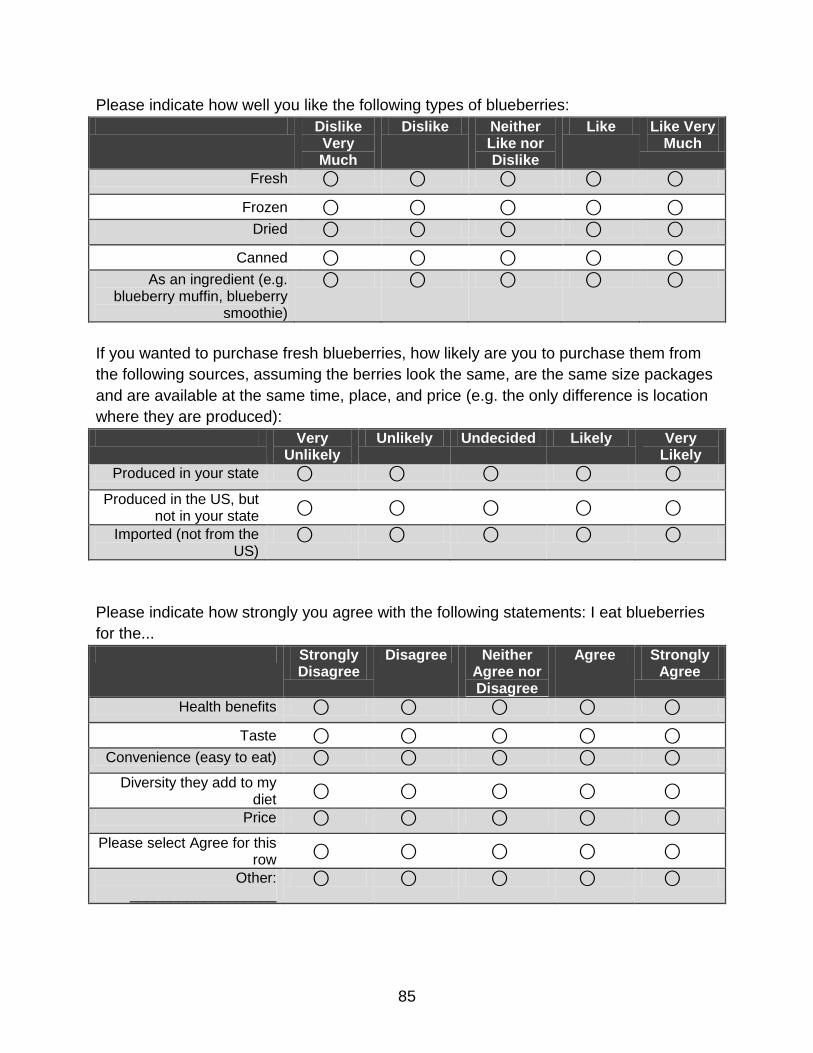
85
Please indicate how well you like the following types of blueberries:
Dislike Very Much
Dislike Neither Like nor Dislike
Like Like Very Much
Fresh ⃝ ⃝ ⃝ ⃝ ⃝
Frozen ⃝ ⃝ ⃝ ⃝ ⃝
Dried ⃝ ⃝ ⃝ ⃝ ⃝
Canned ⃝ ⃝ ⃝ ⃝ ⃝
As an ingredient (e.g. blueberry muffin, blueberry
smoothie)
⃝ ⃝ ⃝ ⃝ ⃝
If you wanted to purchase fresh blueberries, how likely are you to purchase them from
the following sources, assuming the berries look the same, are the same size packages
and are available at the same time, place, and price (e.g. the only difference is location
where they are produced):
Very Unlikely
Unlikely Undecided Likely Very Likely
Produced in your state ⃝ ⃝ ⃝ ⃝ ⃝
Produced in the US, but not in your state
⃝ ⃝ ⃝ ⃝ ⃝
Imported (not from the US)
⃝ ⃝ ⃝ ⃝ ⃝
Please indicate how strongly you agree with the following statements: I eat blueberries
for the...
Strongly Disagree
Disagree Neither Agree nor Disagree
Agree Strongly Agree
Health benefits ⃝ ⃝ ⃝ ⃝ ⃝
Taste ⃝ ⃝ ⃝ ⃝ ⃝
Convenience (easy to eat) ⃝ ⃝ ⃝ ⃝ ⃝
Diversity they add to my diet
⃝ ⃝ ⃝ ⃝ ⃝
Price ⃝ ⃝ ⃝ ⃝ ⃝
Please select Agree for this row
⃝ ⃝ ⃝ ⃝ ⃝
Other: __________________
⃝ ⃝ ⃝ ⃝ ⃝
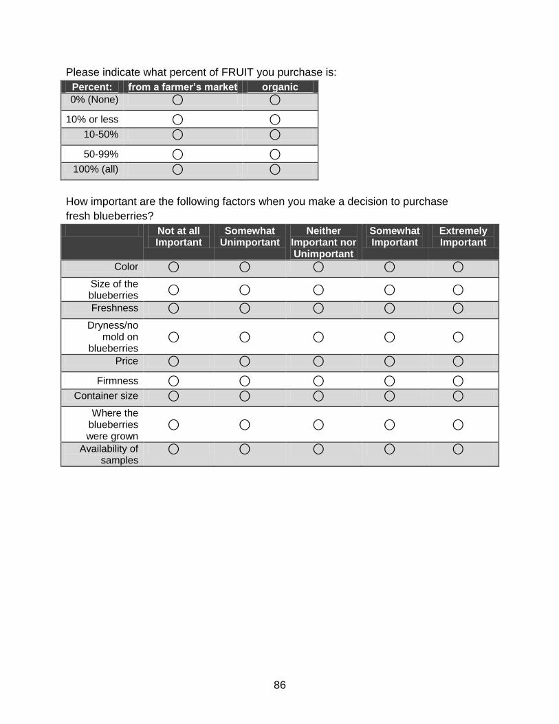
86
Please indicate what percent of FRUIT you purchase is:
Percent: from a farmer’s market organic
0% (None) ⃝ ⃝
10% or less ⃝ ⃝
10-50% ⃝ ⃝
50-99% ⃝ ⃝
100% (all) ⃝ ⃝
How important are the following factors when you make a decision to purchase
fresh blueberries?
Not at all Important
Somewhat Unimportant
Neither Important nor Unimportant
Somewhat Important
Extremely Important
Color ⃝ ⃝ ⃝ ⃝ ⃝
Size of the blueberries
⃝ ⃝ ⃝ ⃝ ⃝
Freshness ⃝ ⃝ ⃝ ⃝ ⃝
Dryness/no mold on
blueberries ⃝ ⃝ ⃝ ⃝ ⃝
Price ⃝ ⃝ ⃝ ⃝ ⃝
Firmness ⃝ ⃝ ⃝ ⃝ ⃝
Container size ⃝ ⃝ ⃝ ⃝ ⃝
Where the blueberries were grown
⃝ ⃝ ⃝ ⃝ ⃝
Availability of samples
⃝ ⃝ ⃝ ⃝ ⃝

87
Please indicate how strongly you agree with the following statements.
Strongly Disagree
Disagree Neither Agree nor Disagree
Agree Strongly Agree
I trust fruits labeled as organic
⃝ ⃝ ⃝ ⃝ ⃝
Organic blueberries are healthier than other
blueberries ⃝ ⃝ ⃝ ⃝ ⃝
I will pay more for fruits with an organic label
⃝ ⃝ ⃝ ⃝ ⃝
I can regularly find organic blueberries
⃝ ⃝ ⃝ ⃝ ⃝
The following questions are used to help us understand how different types of people
have different tastes and preferences. Your responses are anonymous; we do not have
anything that ties your names to your responses. We appreciate your honest answers to
the following questions.
What is your gender?
⃝ Male ⃝ Female
What is your age? _______
What is your ethnicity/race (please select all that apply)?
⃝ Caucasian ⃝ Black or African American
⃝ Hispanic ⃝ Native Hawaiian or Pacific
Islander
⃝ Asian ⃝ American Indian or Alaska Native
⃝ Other ____________________
Please indicate you estimated annual household income:
⃝ Less than $14,999 ⃝ $75,000 - $99,999
⃝ $15,000 - $24,999 ⃝ $100,000 - $149,999
⃝ $25,000 - $34,999 ⃝ $150,000 - $199,999
⃝ $35,000 - $49,999 ⃝ $200,000 or above
⃝ $50,000 - $74,999 ⃝ Do not know
What is your education level?
⃝ Less than high school ⃝ Postgraduate
⃝ High school degree or equivalent ⃝ Trade/technical school
⃝ Some college ⃝ Other ____________________

88
⃝ Four-year college degree ⃝ Don't know
What is your current employment status?
⃝ Full time ⃝ Part time ⃝ Currently not working
⃝ Retired ⃝ Student ⃝ Other
How many people including yourself live in your household?
⃝ 1-2 ⃝ 3-4 ⃝ 5-6 ⃝ 7-8 ⃝ 9 or above
How many children age 18 or younger currently live in your household?
⃝ None ⃝ 1 ⃝ 2 ⃝ 3 ⃝ 4 or more
Approximately how much per week does your family spend on food?
⃝ Less than $49 ⃝ $200-$249
⃝ $50-$99 ⃝ $250-$299
⃝ $100-$149 ⃝ $300 or more
⃝ $150-$199
Please take this survey to an interviewer to complete the last portion of the interview
and receive your gift card.

89
APPENDIX C BDM AUCTION INSTRUCTIONS AND PROCEDURE
We are now interested in your preference for four packages of blueberries typically found at a grocery store. Now, we will conduct an ‘auction’ for the blueberries, where you will have the opportunity to purchase one package of blueberries. In case you do not have cash with you, we are providing you with $7 cash. This cash is yours to keep and is in addition to the $10 gift card you will receive at the end. In a moment, you will be asked to write the most you are willing to pay for each package of blueberries in the spaces below. After you write these amounts, we will auction the blueberries like this: 1. We will randomly draw a letter to determine which blueberry package to actually auction. Even though you will bid on four products, only one will be auctioned. If we draw “A”, we will auction the organic, local blueberries; “B” is for local blueberries; “C” is for organic, produced in the US; and “D” if for produced in the US. It is important to realize that even though you will bid on four products, you will only have the opportunity to buy one package of blueberries. 2. Once we determine which blueberry package will be auctioned, you will randomly draw a ‘secret price’ by selecting a number from this bowl. 3. If your bid for the randomly selected blueberry package is higher than the price from the bowl, then you will purchase the blueberries from me for a price equal to the price from the bowl. Note: payment will actually take place. 4. If your bid for the package is less than the price from the bowl, then you will not purchase the blueberries and will walk away with no blueberries. If you do not wish to purchase one of the blueberry packages, simply bid $0.00 for that package. It is in your best interest to bid exactly what you are willing to pay. For example, if you bid less than it is worth to you to have the blueberries, you might end up not winning the auction even though you could have bought the blueberries at a price you were actually willing to pay. Or, if you bid more than it is worth to you to purchase the blueberries, you may end up having to buy them at a price higher than you really wanted to. Thus it is in your best interest to bid exactly what you are willing to pay. Do you have any questions? The most I am willing to pay for…
A. Organic, Locally produced Blueberries is $________
B. Locally produced Blueberries is $________
C. Organic, produced in the US Blueberries is $________

90
D. Blueberries produced in the US is $________
91
LIST OF REFERENCES
Alfnes, F., A. G. Guttormsen, G. Steine, and K. Kolstad. “Consumers’ Willingness to Pay for the Color of Salmon: A Choice Experiment with Real Economic Incentives.” American Journal of Agricultural Economics 88(2006):1050-1061.
Alfnes, F. “Stated Preferences for Imported and Hormone-treated Beef: Application of a Mixed Logit Model.” European Review of Agricultural Economics 31(2004):19-37.
Alfnes, F. and K. Rickertsen. “European Consumers’ Willingness to Pay for U.S. Beef in Experimental Auction Markets.” American Journal of Agricultural Economics 85(2003):396-405.
Allenby, G. and P. Rossi. “Marketing Models of Consumer Heterogeneity.” Journal of Econometrics 89(1998):57-78.
Balcombe, K., A. Chalak, and I. Fraser. “Model Selection for the Mixed Logit with Bayesian Estimation.” Journal of Environmental Economics and Management 57(2009):226-237.
Balcombe. K., L. Fraser, and L. Harris. “Consumer Willingness to Pay for In-flight Service and Comfort Levels: A Choice Experiment.” Journal of Air Transport Management 15(2009):221-226.
Batte, M. T., N. H. Hooker, T. C. Haab, and J. Beaverson. “Putting Their Money where Their Mouths are: Consumer Willingness to Pay for Multi-ingredient, Processed Organic Food Products.” Food Policy 32(2007):145-159.
Becker, G. M., M. H. Degroot, and J. Marschak. “Measuring Utility by a Single‐response Sequential Method.” Behavioral Science 9(1964):226-232.
Bernard, J. C. and D. J. Bernard. “Comparing Parts with the Whole: Willingness to Pay for Pesticide-Free, Non-GM, and Organic Potatoes and Sweet Corn.” Journal of Agricultural and Resource Economics 35(2010):457-475.
Bettman, J. R., M. F. Luce, and J. W. Payne. “Constructive Consumer Choice Processes.” The Journal of Consumer Research 25(1998):187-217.
Birol, E., K. Karousakis, and P. Koundouri. “Using a Choice Experiment to Account for Preference Heterogeneity in Wetland Attributes: The Case of Cheimaditida Wetland in Greece.” Ecological Economics 60(2006):145-156.
Bond, C. A., D. D. Thilmany, and J. K. Bond. “What to Choose? The Value of Label Claims to Fresh Produce Consumers.” Journal of Agricultural and Resource Economics 33(2008):402-427.
92
Brooks, K. and J. L. Lusk. “Stated and Revealed Preferences for Organic and Cloned Milk: Combining Choice Experiment and Scanner Data.” American Journal of Agriculture Economics 92(2010):1229-1241.
Carlsson, F., P. Frykblom, and C. J. Lagerkvist. “Consumer Benefits of Labels and Bans on Genetically Modified Food- An Empirical Analysis Using Choice Experiment.”, 2004. Working Paper in Economics no. 129, Department of Economics, Gothenburg University.
Carson, R. T., J. J. Louviere, D. A. Anderson, P. Arabie, D. S. Bunch, D. A. Hensher, R. M. Johnson, W. F. Kuhfeld, D. Steinberg, J. Swait, H. Timmermans, and J. B. Wiley. "Experimental Analysis of Choice." Marketing Letters 5(1994):351-368.
Casella, G. and E. I. George. “Explaining the Gibbs Sampler.” The American Statistician 46(1992):167-174.
Corrigan, J. R. and M. C. Rousu. “Testing Whether Field Auction Experiments Are Demand Revealing in Practice.” Journal of Agricultural and Resource Economics 33(2008):290-301.
Darby, K., M. T. Batte, S. Ernst, and B. Roe. “Willingness to Pay for Locally Produced Foods: A Customer Intercept Study of Direct Market and Grocery Store Shoppers.” American Agricultural Economics Association Annual Meeting, Long Beach, California, July 23-26, 2006.
Dentoni, D., G. T. Tonsor, R. J. Calantone, and H. C. Peterson. “The Direct and Indirect Effects of “Locally Grown” on Consumers’ Attitudes towards Agri-Food Products.” Agricultural and Resource Economics Review 38(2009):384-396.
Fox, J. A., J. F. Shogren, D. J. Hayes, and J. B. Kliebenstein. “CVM-X: Calibrating Contingent Values with Experimental Auction Markets.” American Journal of Agricultural Economics 80(1998):455-465.
Frank, R. E., W. F. Massy, and H. W. Boyd. “Correlates of Grocery Product Consumption Rates.” Journal of Marketing Research 4(1967):184-190.
Gao, Z. and T. Schroeder. “Effects of Additional Quality Attributes on Consumer Willingness-to-pay for Food Lables.” AAEA, WAEA, and CAES Joint Annual Meeting, Portland, Oregon, July 29-August 1, 2007.
Hanley, N., R. E. Wright, and V. Adamowicz. “Using Choice Experiments to Value the Environment.” Environmental and Resource Economics 11(1998):413-428.
Hayes, D. J., J. F. Shogren, S. Y. Shin, and J. B. Kliebenstein. “Valuing Food Safety in Experimental Auction Markets.” American Journal of Agricultural Economics 77(1995):40-53.
93
Hensher, D. A., W. H. Greene, and J. M. Rose. “Deriving Willingness-to-pay Estimates of Travel-time Savings from Individual-based Parameters.” Environment and Planning 38(2006):2365-2376.
Hensher, D. A. and W. H. Greene. “Valuation of Travel Time Savings in WTP and Preference Space in the Presence of Taste and Scale Heterogeneity.” Journal of Transport Economics and Policy 45(2011):505-525.
Hensher, D. A., N. Shore, and K. Train. “Households’ Willingness to Pay for Water Service Attributes.” Environmental and Resource Economics 32(2005):509-531.
Horowitz, J. K. "The Becker-DeGroot-Marschak Mechanism is not Necessarily Incentive Compatible, even for Non-random Goods." Economic Letters 93 (2006):6-11.
Hu, W., T. Woods, and S. Bastin. “Consumer Acceptance and Willingness to Pay for Blueberry Products with Nonconventional Attributes.” Journal of Agricultural and Applied Economics 41(2009):47-60.
Hu, W., T. Woods, S. Bastin, L. Cox, and W. You. “Assessing Consumer Willingness to Pay for Value-Added Blueberry Products Using a Payment Card Survey.” Journal of Agricultural and Applied Economics 43(2011):243-258.
Huber. J. and K. Train. “On the Similarity of Classical and Bayesian Estimates of Individual Mean Partworths.” Marketing Letters 12(2001):259-269.
Huffman, W. E., J. F. Shogren, M. Rousu, and A. Tegene. "Consumer Willingness to Pay for Genetically Modified Food Labels in a Market with Diverse Information: Evidence from Experimental Auctions." Journal of Agricultural and Resource Economics 28(2003):481-502.
Irwin, J. R., P. Slovic, S. Lichtenstein, and G. H. McClelland."Preference Reversals and the Measurement of Environmental Values." Journal of Risk and Uncertainty 6(1993):5–18.
Jaeger, S. R., J. L. Lusk, L. O. House, C. Valli, M. Moore, B. Morrow, and W. B. Traill. “The Use of Non-hypothetical Experimental Markets for Measuring the Acceptance of Genetically Modified Foods.” Food Quality and Preference 15(2004):701-714.
Janssen, M., A. Heid, and U. Hamm. “Is There a Promising Market ‘in between’ Organic and Conventional Food? Analysis of Consumer Prefernces.” Renewable Agriculture and Food Systems 24(2009):205-213.
Johansson-Stenman, O. and H. Svedsäter. “Measuring Hypothetical Bias in Choice Experiments: The Importance of Cognitive Consistency.” The B.E. Journal of Economic Analysis & Policy 8(2008).
94
Layton, D. F. and G. Brown. “Heterogeneous Preferences Regarding Global Climate Change.” The Review of Economics and Statistics 82(2000):616-624.
Lin, B., T. A. Smith, and C. L. Huang. “Organic Premiums of US Fresh Produce.” Renewable Agriculture and Food Systems 23(2008):208-216.
List, J. A. “Do Explicit Warnings Eliminate the Hypothetical Bias in Elicitation Procedures? Evidence from Field Auctions for Sportscards.” The American Economic Review 91(2001):1498-1507.
List, J. A. “Preference Reversals of a Different Kind: The ‘More Is Less’ Phenomenon.” The American Economic Review 92(2002):1636-1643.
List, J. A. and C. A. Gallet. “What Experimental Protocol Influence Disparities between Actual and Hypothetical Stated Values?” Environmental and Resource Economics 20(2001):241–254.
List, J. A. and D. Lucking-Reiley. “Demand Reduction in Multiunit Auctions: Evidence from a Sportscard Field Experiment.” The American Economic Review 90(2000):961-972.
List, J. A, and J. F. Shogren. “Calibration of the Difference between Actual and Hypothetical Valuations in a Field Experiment.” Journal of Economic Behavior & Organization 37(1998):193–205.
Loureiro, M. L., J. J. McCluskey, and R. C. Mittelhammer. “Assessing Consumer Preferences for Organic, Eco-labeled, and Regular Apples.” Journal of Agricultural and Resource Economics 26(2001):404-416.
Lusk, J. L. and J. A. Fox. “Value Elicitation in Retail and Laboratory Environments.” Economics Letters 79(2003):27-34.
Lusk, J. L., J. A. Fox, T. C. Schroeder, J. Mintert, and M. Koohmaraie. "In-store Valuation of Steak Tenderness." American Journal of Agricultural Economics 83(2001):539–550.
Lusk, J. L., L. O. House, C. Valli, S. R. Jaeger, M. Moore, J. L. Morrow, and W. B. Traill. “Effect of Information about Benefits of Biotechnology on Consumer Acceptance of Genetically Modified Food: Evidence from Experimental Auctions in the United States, England, and France.” European Review of Agricultural Economics 31(2004):179-204.
Lusk, J. L., T. Nilsson, and K. Foster. “Public Preferences and Private Choices: Effect of Altruism and Free Riding on Demand for Environmentally Certified Pork.” Environmental and Resource Economics 36(2007):499-521.
95
Lusk, J. L. and B. Norwood. “Effect of Experimental Design on Choice-Based Conjoint Valuation Estimates.” American Journal of Agricultural Economics 87(2005):771-785.
Lusk, J. L., J. Roosen, and J. A. Fox. “Demand for Beef from Cattle Administered Growth Hormones or Fed Genetically Modified Corn: A Comparison of Consumers in France, Germany, the United Kingdom, and the United States.” American Journal of Agricultural Economics 85(2003):16-29.
Lusk, J. L. and T. C. Schroeder. “Are Choice Experiments Incentive Compatible? A Test with Quality Differentiated Beef Steaks.” American Journal of Agricultural Economics 86(2004):467-482.
Managi, S., Y. Yamamoto, H. Iwamoto, and K. Masuda. “Valuing the Influence of Underlying Attitudes and the Demand for Organic Milk in Japan.” Agricultural Economics 39(2008):339-348.
McFadden, D. L. and K. Train. “Mixed MNL Models for Discrete Response.” Journal of Applied Econometrics 15(2000):447-470.
Melton, B. E., W. E. Huffman, J. F. Shogren, and J. A. Fox. “Consumer Preferences for Fresh Food Items with Multiple Quality Attributes: Evidence from an Experimental Auction of Pork Chops.” American Journal of Agricultural Economics 78(1996):916-923.
Ӧzdemir, S., F. R. Johnson, and A. B. Hauber. “Hypothetical Bias, Cheap Talk, and Stated Willingness to Pay for Health Care.” Journal of Health Economics 28(2009):894-901.
Payne, J. W., J. R. Bettman, and E. J. Johnson. "Behavioral Decision Research: A Constructive Processing Perspective." Annual Review of Psychology 43 (1992):87-131.
Provencher, B. and R. C. Bishop. “Does Accounting for Preference Heterogeneity Improve the Forecasting of a Random Utility Model? A Case Study.” Journal of Environmental Economics and Management 48(2004):793-810.
Revelt, D. and K. Train. “Mixed Logit with Repeated Choices: Households’ Choices of Appliance Efficiency Level.” Review of Economics and Statistics 80(1998):647-657.
Revelt, D. and K. Train. “Consumer-Specific Taste Parameters and Mixed Logit: Households’ Choice of Electricity Supplier.”, 2000. Working Paper No. E00-274, Department of Economics, University of California at Berkeley.
Robert, C. P. and G. Casella. Monte Carlo Statistical Methods. Springer, 2004.
96
Rossi, P. E. and G. M. Allenby. “Bayesian Statistics and Marketing.” Marketing Science 22(2003):304-328.
Rossi, P. E., G. M. Allenby, and R. E. McCulloch. Bayesian Statistics and Marketing. Wiley, 2005.
Rossi, P. E., R. E. McCulloch, and G. M. Allenby. “The Value of Purchase History Data in Target Marketing.” Marketing Science 15(1996):321-340.
Rousu, M. C., D. C. Monchuk, J. F. Shogren, and K. M. Kosa. “Consumer Willingness to Pay for ‘Second-Generation’ Genetically Engineered Products and the Role of Marketing Information.” Journal of Agricultural and Applied Economics 37(2005):647-657.
Rozan, A., A. Stenger, and M. Willinger. “Willingness-to-Pay for Food Safety: An Experimental Investigation of Quality Certification on Bidding Behaviour.” European Review of Agricultural Economics 31(2004):409-425.
Ruud, P. “Simulation of the Multinomial Probit Model: An Analysis of Covariance Matrix Estimation.”, 1996. Working Paper, Department of Economics, University of California.
Scarpa, R., M. Thiene, and K. Train. “Utility in Willingness to Pay Space: A Tool to Address Confounding Random Scale Effects in Destination Choice to the Alps.” American Journal of Agricultural Economics 90(2008):994-1010.
Scarpa, R. and K. Willis. “Willingness-to-Pay for Renewable Energy: Primary and Discretionary Choice of British Households' for Micro-Generation Technologies.” Energy Economics 32(2010):129-136.
Shogren, J. F., J. A. Fox, D. J. Hayes, and J. Roosen. “Observed Choices for Food Safety in Retail, Survey, and Auction Markets.” American Journal of Agricultural Economics 81(1999):1192-1199.
Silva, A., R. M. Nayga, Jr., B. L. Campbell, and J. L. Park. “On the Use of Valuation Mechanisms to Measure Consumers’ Willingness to Pay for Novel Products: A Comparison of Hypothetical and Non-Hypothetical Values.” International Food and Agribusiness Management Review 10(2007):165-180.
Sonnier, G., A. Ainslie, and T. Otter. “Heterogeneity Distributions of Willingess-to-pay in Choice Models.” Quantitative Marketing and Economics 5(2007):313-331.
Thaler. R. "Mental Accounting and Consumer Choice." Marketing Science 4(1985):199-214.
Thiene. M. and R. Scarpa. “Deriving and Testing Efficient Estimates of WTP Distributions in Destination Choice Models.” Environmental and Resource Economics 44(2009):379-395.
97
Train, K. Discrete Choice Methods with Simulation. Cambridge: Cambridge University Press, 2003.
Train, K. and M. Weeks. “Discrete Choice Models in Preference Space and Willingness-to-Pay Space.” Application of Simulation Methods in Environmental and Resource Economics. R. Scarpa and A. Alberini, eds. Dordrecht, The Netherlands: Springer Publisher, 2005, Chapter 1, pp. 1-16.
Tversky, A. and I. Simonson. "Context-dependent Preferences." Management Science 39(1993):1179-1189.
Umberger, W. J., D. M. Feuz, C. R. Calkins, and K. Killinger‐Mann. “U.S. Consumer preference and Willingness‐to‐Pay for Domestic Corn‐Fed Beef versus
International Grass‐Fed Beef Measured through an Experimental Auction.” Agribusiness 18(2002):491-504.
Umberger, W. J., D. M. Feuz, C. R. Calkins, and B. M. Sitz. “Country-Of-Origin Labeling of Beef Products: U.S. Consumers' Perceptions.” Journal of Food Distribution Research 34(2003):103-116.
USDA, Economics, Statistics, and Market Information System, Economic Research Service, U.S. Blueberry Industry. Available online at: http://usda.mannlib.cornell.edu/MannUsda/viewDocumentInfo.do?documentID=1765 (Accessed June 02, 2010).
Wang, Q. and J. Sun. “Consumer Preference and Demand for Organic food: Evidence from a Vermont Survey.” 2003. Paper presented at American Agricultural Economics Association 2003 Annual Meetings, Montreal, Canada.
Wedel, M., W. Kamakura, N. Arora, A. Bemmaor, J. Chiang, T. Elrod, R. Johnson, P. Lenk, S. Neslin and C. S. Poulsen. “Discrete and Continuous Representations of Unobserved Heterogeneity in Choice Modeling.” Marketing Letters 10(1999):219-232.
Wertenbroch, K. and B. Skiera. “Measuring Consumers' Willingness to Pay at the Point of Purchase.” Journal of Marketing Research 39(2002):228-241.
Yankelovich, D. “New Criteria for Market Segmentation.” Harvard Business Review 42(1964):83-90.
Yue, C. and C. Tong. “Organic or Local? Investigating Consumer Preference for Fresh Produce Using a Choice Experiment with Real Economic Incentives.” Hortscience 44(2009):366-371.

98
BIOGRAPHICAL SKETCH
Lijia Shi received her Ph.D. in food and resource economics at the University of
Florida in 2012. She also holds a master’s degree in applied economics from the City
University of Hong Kong and a bachelor’s degree in environmental engineering from
Shanghai Jiao Tong University. Lijia’s research interests focus on market research,
consumer behavior, survey design and quantitative methodologies.